
Integration of Geostatistical and Sentinal-2AMultispectral Satellite Image Analysis for Predicting Soil Fertility Condition in Drylands

 , , ,
, , ,  and
and
Abstract
:1. Introduction
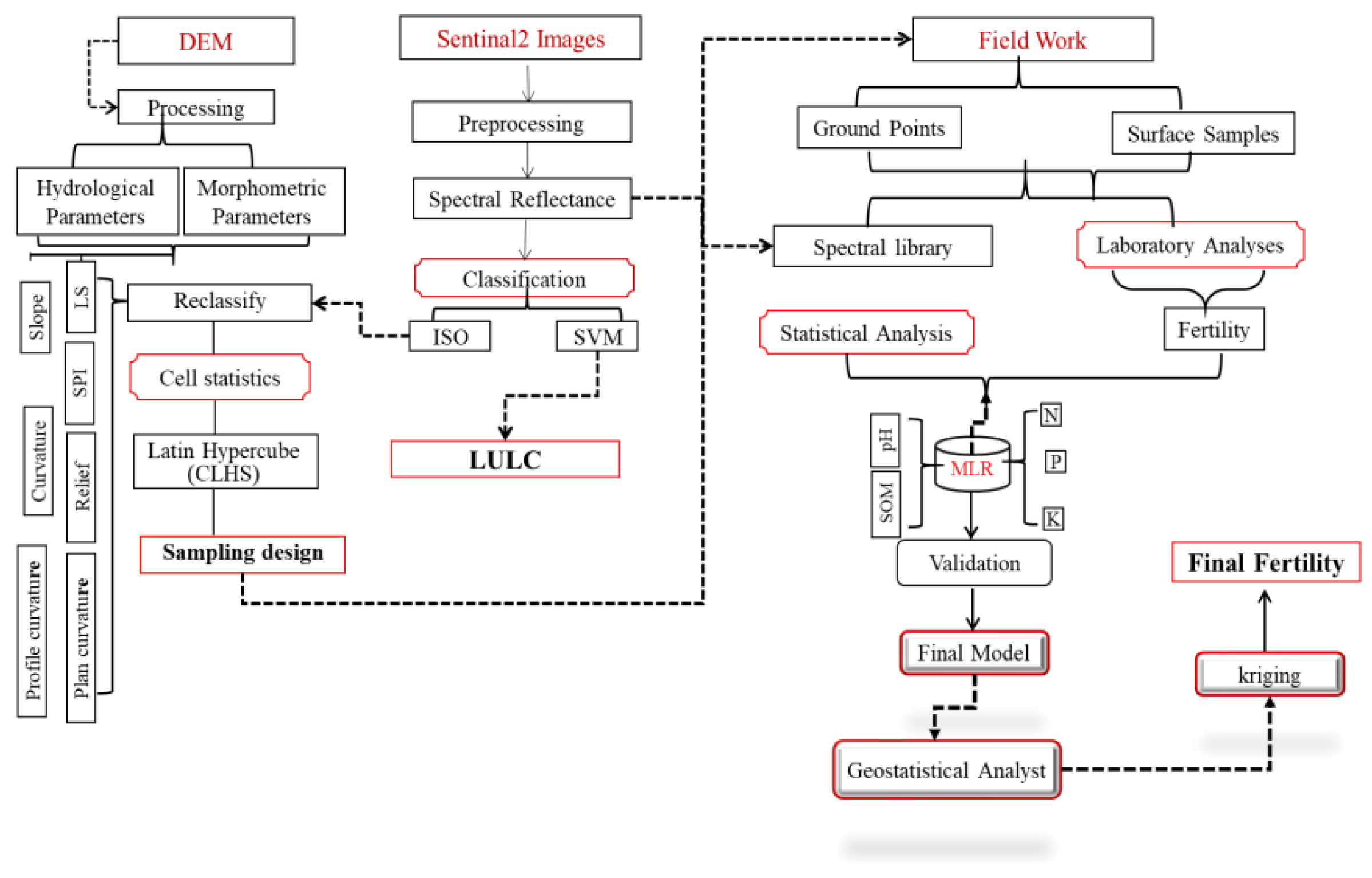
2. Materials and Methods
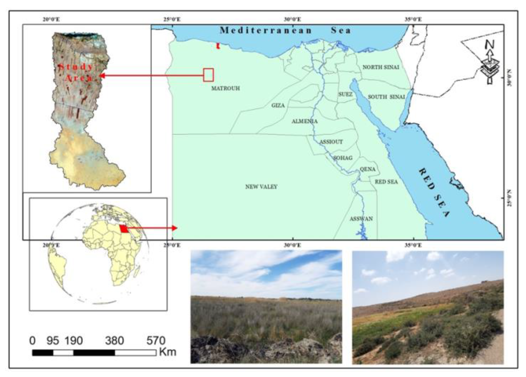
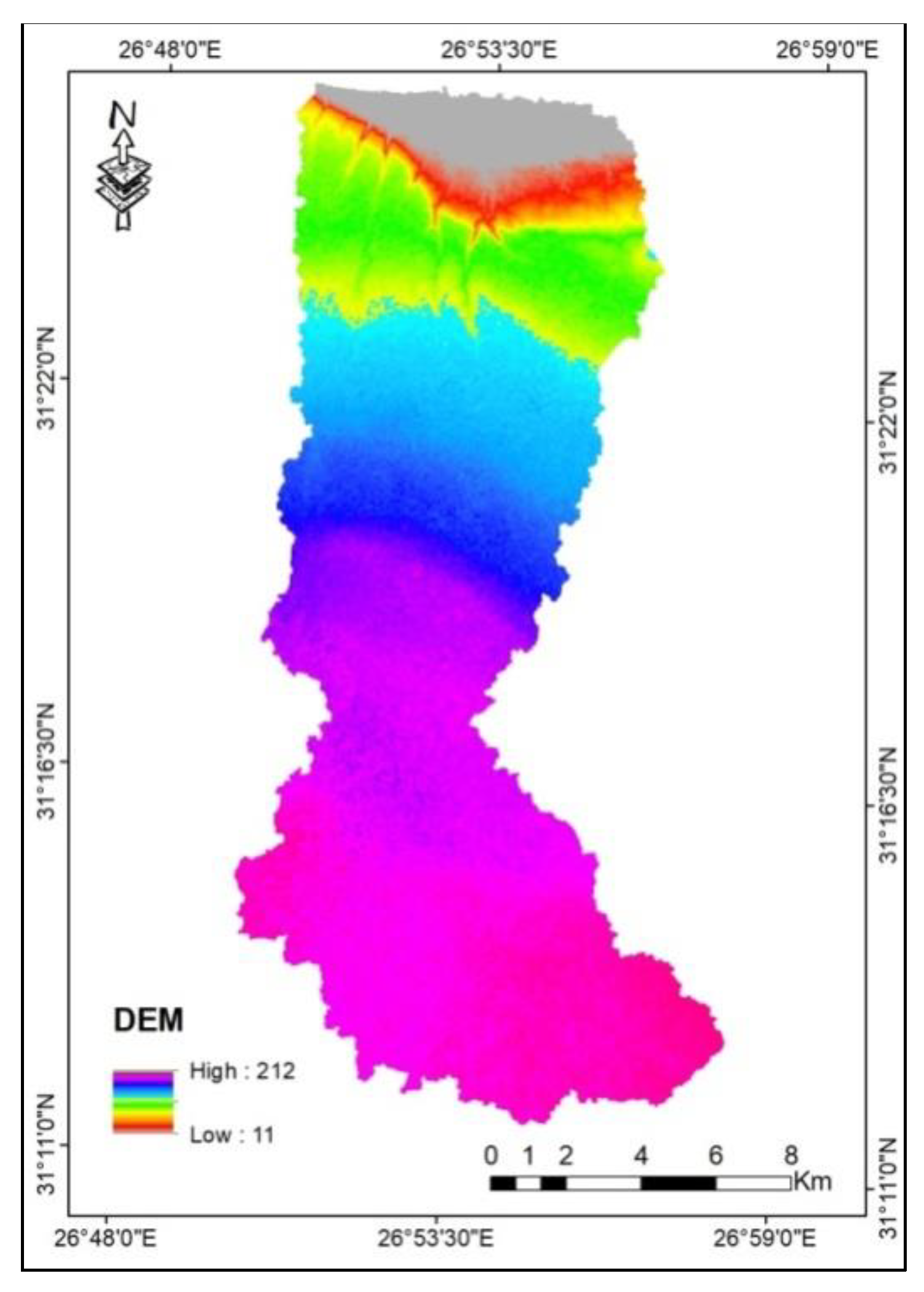
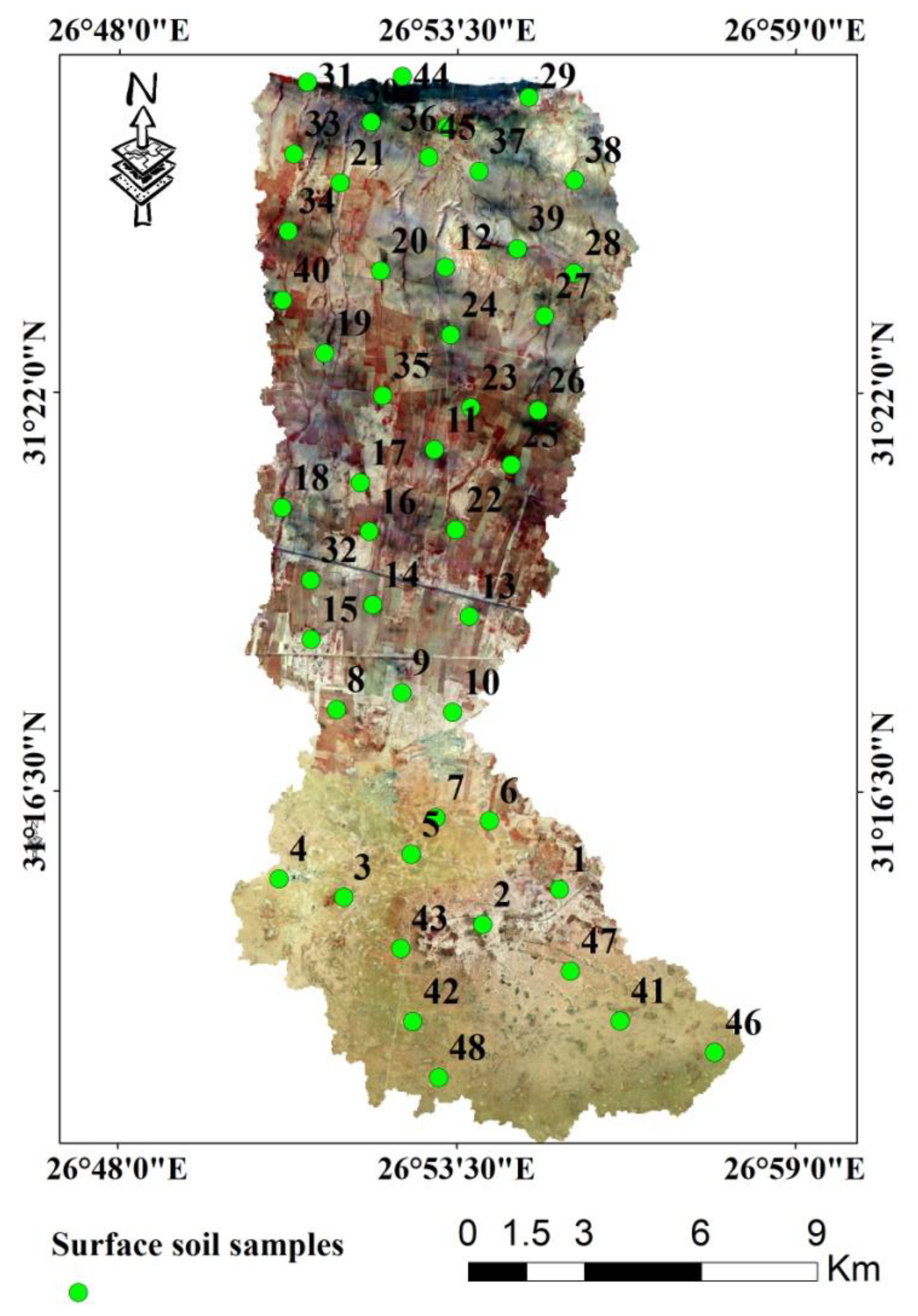
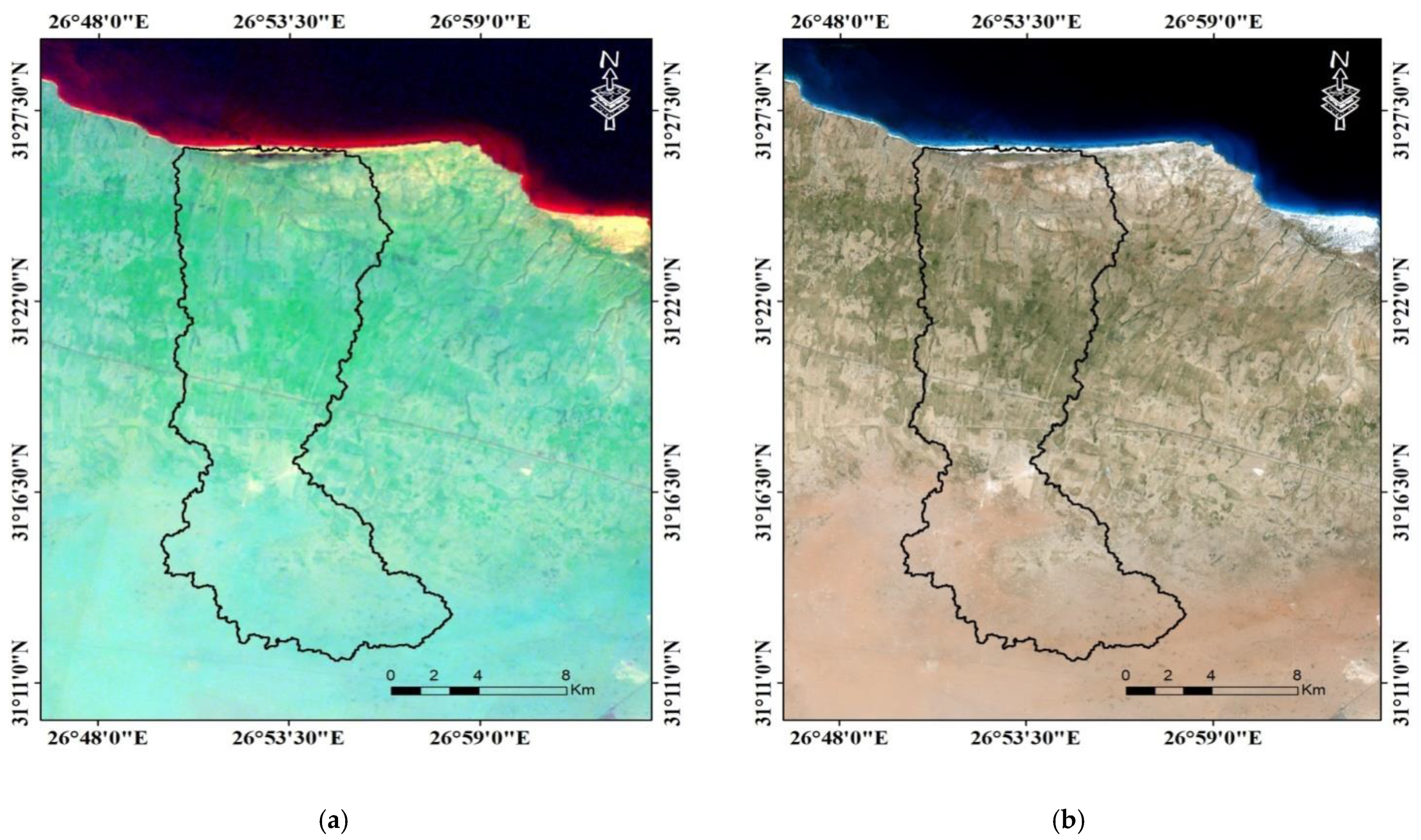
2.1. Study Area
2.2. Soil Sampling and Laboratory Analysis
2.3. Digital Image Processing
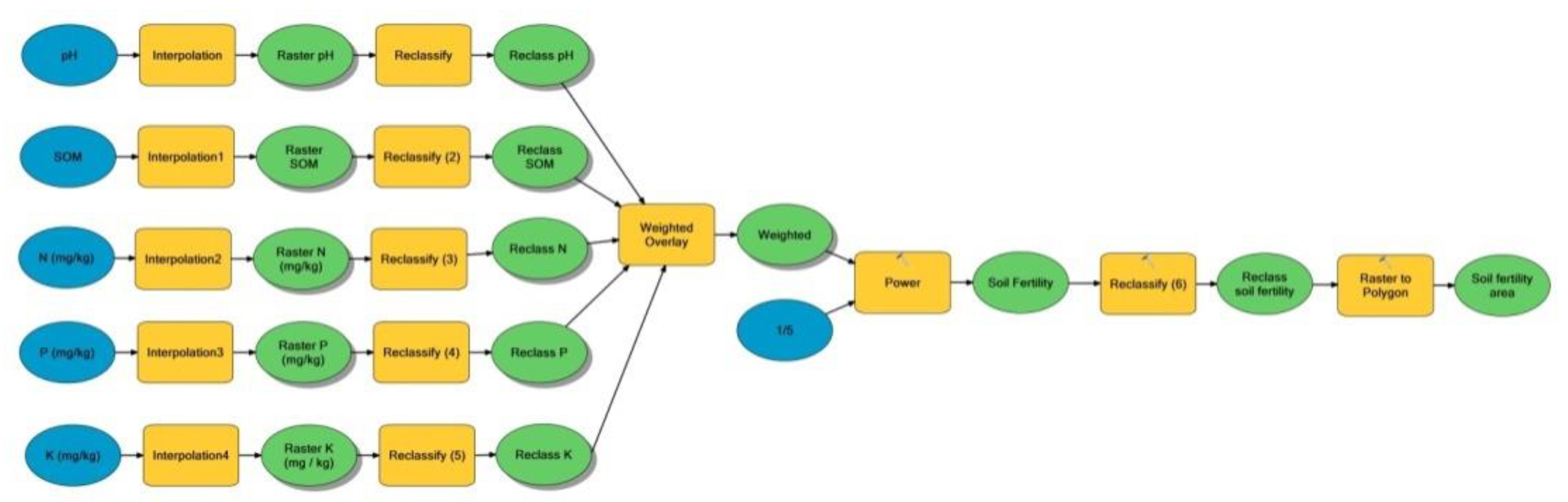
2.4. Procedure of Modelling
2.5. Producing Maps of Soil Properties
2.6. Modelling of SFC in the Study Area
3. Results and Discussion
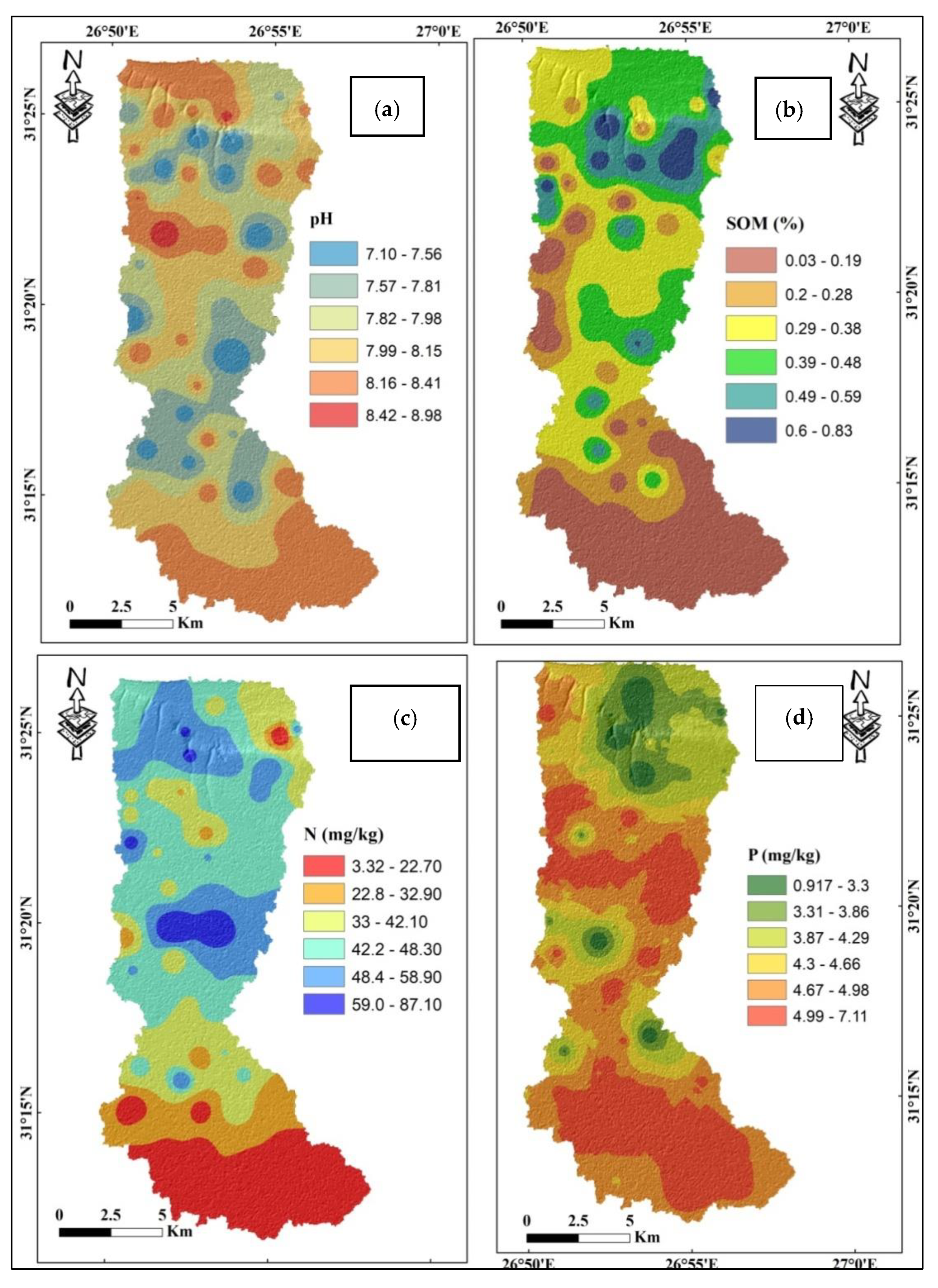
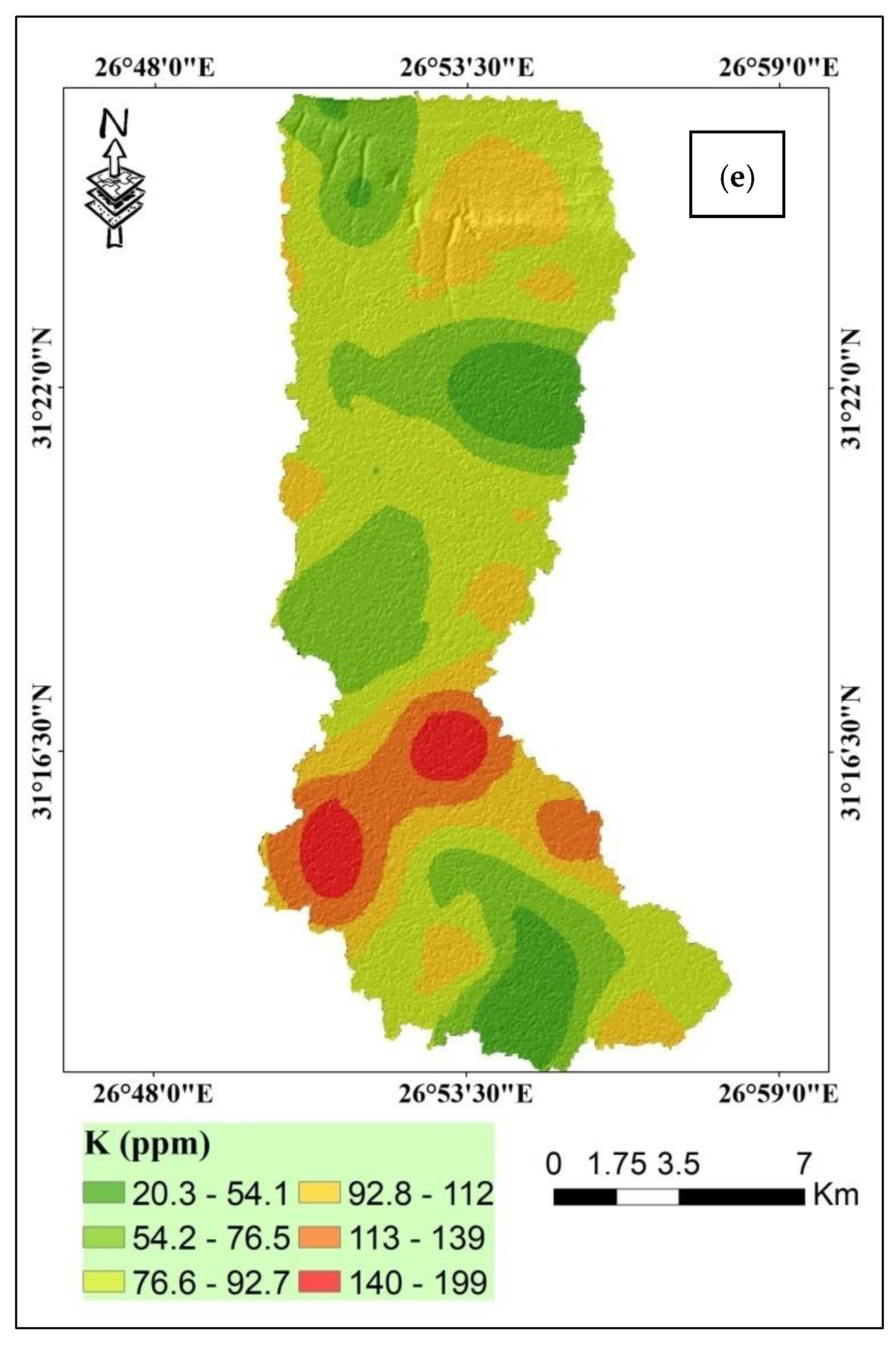
3.1. Soil Properties
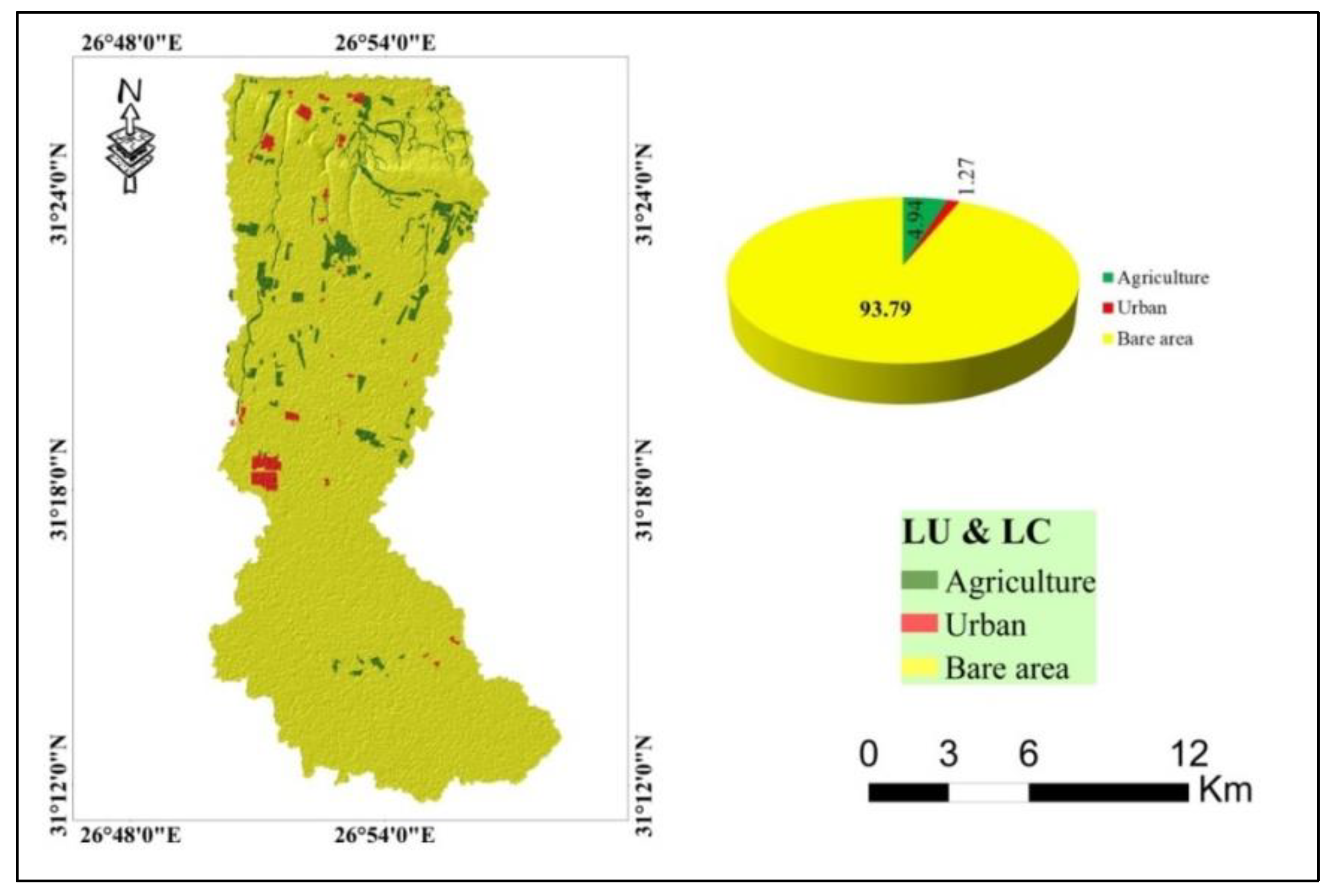
3.2. Producing SFC Parameter Using S2A Image
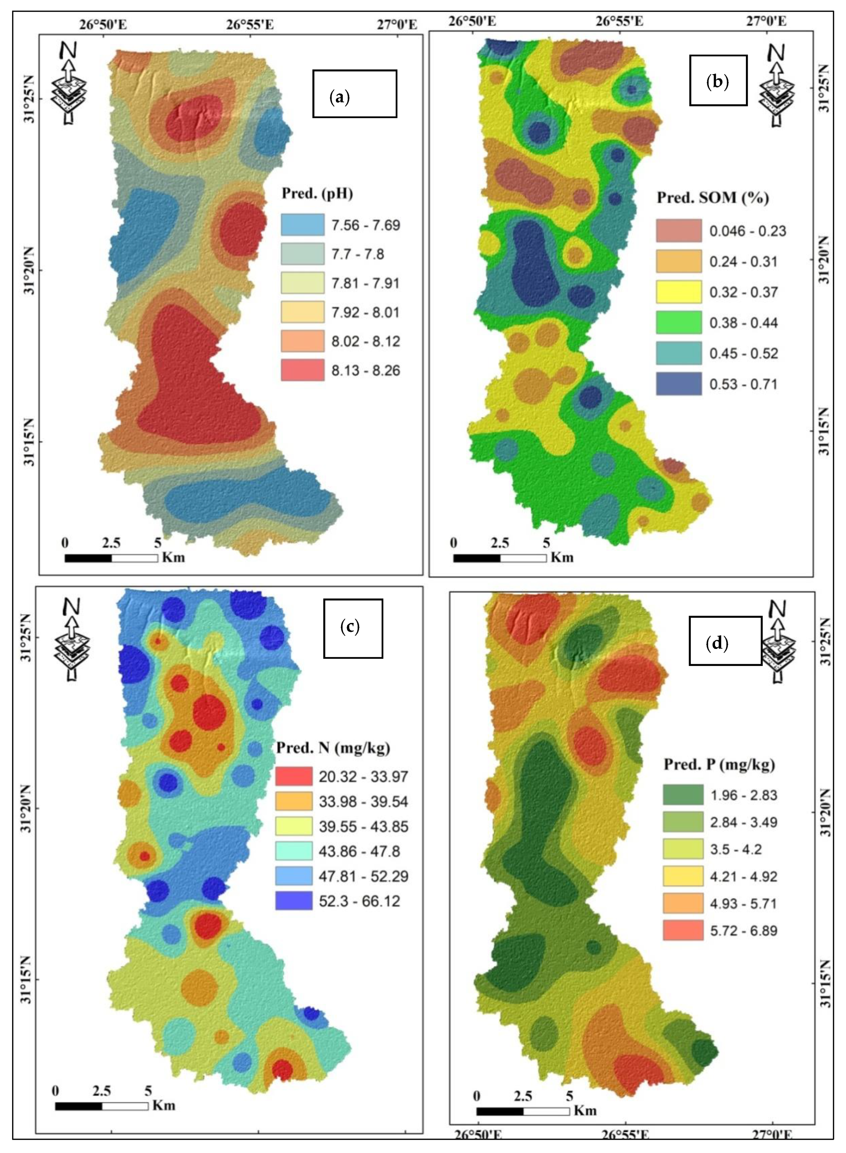
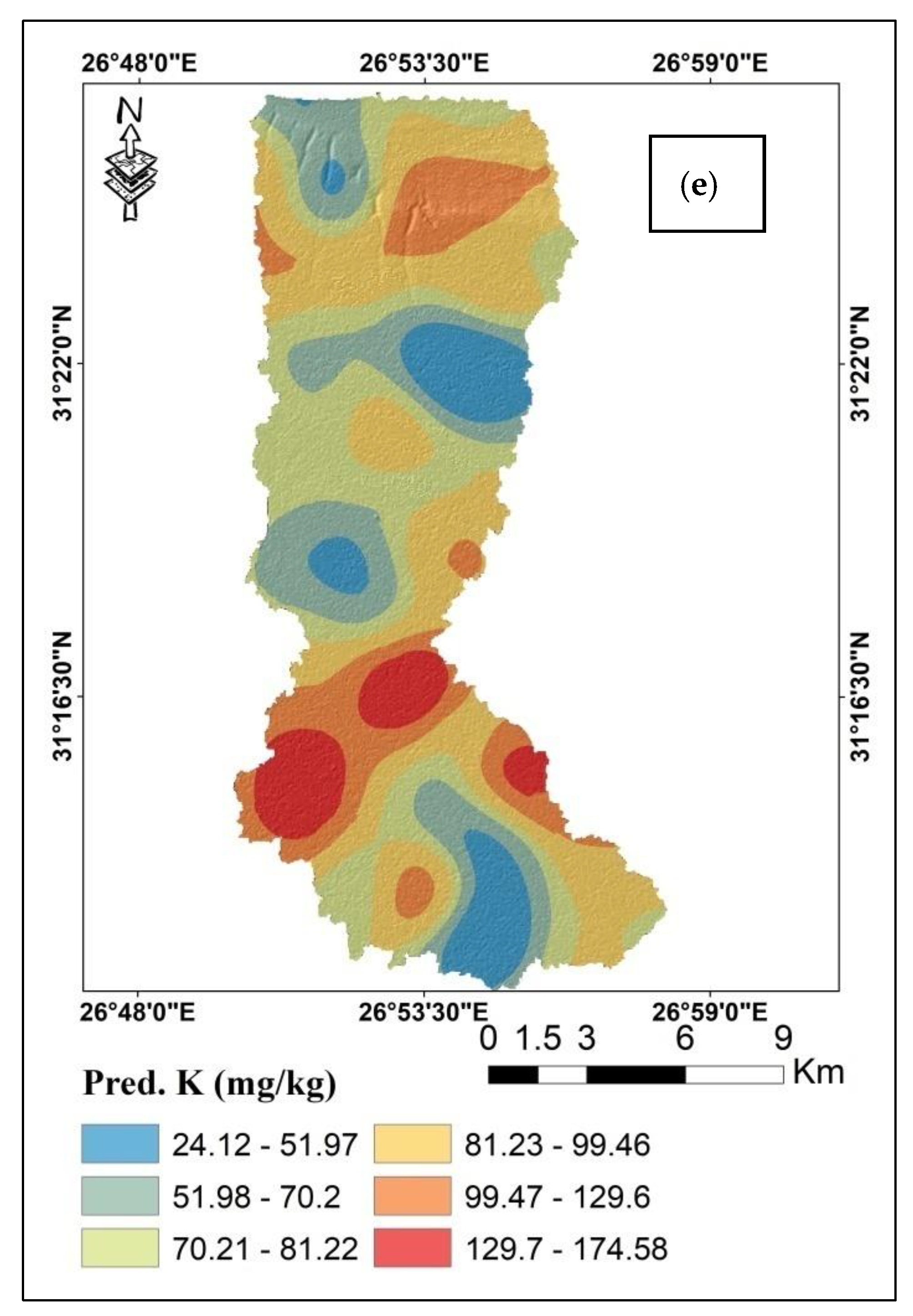
3.3. Spatial Distribution of Predicted SOC Parameters Based on OK
3.4. Multivariate Statistical Analysis (MSA)
3.5. The SFC of Study Area
4. Conclusions
Supplementary Materials
Author Contributions
Funding
Institutional Review Board Statement
Informed Consent Statement
Data Availability Statement
Acknowledgments
Conflicts of Interest
References
- Mohamed, E.S.; Abu-Hashim, M.; Belal, A.A.A. Sustainable Indicators in Arid Region: Case Study–Egypt. In Sustainability of Agricultural Environment in Egypt Soil-Water-Food Nexus, The Handbook of Environmental Chemistry; Springer Science and Business Media LLC: Berlin/Heidelberg, Germany, 2018; pp. 273–293. [Google Scholar]
- AbdelRahman, M.A.; Shalaby, A.; Mohamed, E.S. Comparison of two soil quality indices using two methods based on geographic information system. Egypt J. Remote Sens. Space Sci. 2019, 22, 127–136. [Google Scholar] [CrossRef]
- Abu-hashim, M.; Elsayed, M.; Belal, A.E. Effect of land-use changes and site variables on surface soil organic carbon pool at Mediterranean Region. J. Afr. Earth Sci. 2016, 114, 78–84. [Google Scholar] [CrossRef]
- Hendawy, E.; Belal, A.A.; Mohamed, E.S.; Elfadaly, A.; Murgante, B.; Aldosari, A.A.; Lasaponara, R. The prediction and assessment of the impacts of soil sealing on agricultural land in the North Nile Delta (Egypt) using satellite data and GIS modeling. Sustainability 2019, 11, 4662. [Google Scholar] [CrossRef] [Green Version]
- Vaudour, E.; Gomez, Y.C.; Fouad, P. Lagacherie, Sentinel-2 image capacities to predict common topsoil properties of temperate and Mediterranean agroecosystems. Remote Sens. Environ. 2019, 223, 21–33, ISSN 0034-4257. [Google Scholar] [CrossRef]
- Mohamed, E.S.; Baroudy, A.A.E.; El-beshbeshy, T.; Emam, M.; Belal, A.A.; Elfadaly, A.; Aldosari, A.A.; Ali, A.M.; Lasaponara, R. Vis-NIR Spectroscopy and Satellite Landsat-8 OLI Data to Map Soil Nutrients in Arid Conditions: A Case Study of the Northwest Coast of Egypt. Remote Sens. 2020, 12, 3716. [Google Scholar] [CrossRef]
- Horta, A.; Malone, B.; Stockmann, U.; Minasny, B.; Bishop, T.F.A.; McBratney, A.B.; Pallasser, R.; Pozza, L. Potential of integrated field spectroscopy and spatial analysis for enhanced assessment of soil contamination: A prospective review. Geoderma 2015, 241, 180–209. [Google Scholar] [CrossRef] [Green Version]
- Angelopoulou, T.; Tziolas, N.; Balafoutis, A.; Zalidis, G.; Bochtis, D. Remote sensing techniques for soil organic carbon estimation: A review. Remote Sens. 2019, 11, 676. [Google Scholar] [CrossRef] [Green Version]
- Minasny, B.; McBratney, A.B. A conditioned Latin hypercube method for sampling in the presence of ancillary information. Comput. Geosci. 2006, 32, 1378–1388. [Google Scholar] [CrossRef]
- Brungard, C.W.; Boettinger, J.L. Conditioned Latin hypercube sampling: Optimal sample size for digital soil mapping of arid Rangelands in Utah, USA. In Digital Soil Mapping; Boettinger, J.L., Howell, D.W., Moore, A.C., Hartemink, A.E., Kienast-Brown, S., Eds.; Progress in Soil Science; Springer: Dordrecht, The Netherlands, 2010. [Google Scholar]
- Brungard, C.W.; Boettinger, J.L.; Duniway, M.C.; Wills, S.A.; Edwards, T.C., Jr. Machine learning for predicting soil classes in three semi-arid landscapes. Geoderma 2015, 239–240, 68–83. [Google Scholar] [CrossRef] [Green Version]
- Worsham, L.; Markewitz, D.; Nibbelink, N.P.; West, L.T. A comparison of three field sampling methods to estimate soil carbon content. Forest Sci. 2012, 58, 513–522. [Google Scholar] [CrossRef]
- Taghizadeh-Mehrjardi, R.; Nabiollahi, K.; Minasny, B.; Triantafilis, J. Comparing data mining classifiers to predict spatial distribution of USDA-family soil groups in Baneh region, Iran. Geoderma 2015, 253–254, 67–77. [Google Scholar] [CrossRef]
- Levi, M.R.; Rasmussen, C. Covariate selection with iterative principal component analysis for predicting physical soil properties. Geoderma 2014, 219, 46–57. [Google Scholar] [CrossRef]
- Taghizadeh-Mehrjardi, R.; Minasny, B.; Sarmadian, F.; Malone, B.P. Digital mappingof soil salinity in Ardakan region, central Iran. Geoderma 2014, 213, 15–28. [Google Scholar] [CrossRef]
- Lacoste, D.; Gaspard, P. Isometric fluctuation relations for equilibrium states with broken symmetry. Phys. Rev. Lett. 2014, 113, 24. [Google Scholar] [CrossRef] [Green Version]
- Scarpone, C.; Schmidt, M.G.; Bulmer, C.E.; Knudby, A. Modelling soil thickness in the critical zone for Southern British Columbia. Geoderma 2016, 282, 59–69. [Google Scholar] [CrossRef]
- Waruru, B.K.; Shepherd, K.D.; Ndegwa, G.M.; Sila, A.M. Estimation of wet aggregation: Indices using soil properties and diffuse reflectance near infrared spectroscopy, an application of classification and regression tree analysis. Biosyst. Eng. 2016, 152, 148–164. [Google Scholar] [CrossRef]
- Adhikari, K.; Hartemink, A.E. Soil organic carbon increases under intensive agriculture in the Central Sands, Wisconsin, USA. Geoderma Reg. 2017, 10, 115–125. [Google Scholar] [CrossRef]
- Domenech, M.B.; Castro-Franco, M.; Costa, J.L.; Amiotti, N.M. Sampling scheme optimization to map soil depth to petrocalcic horizon at field scale. Geoderma 2017, 290, 75–82. [Google Scholar] [CrossRef]
- Jeong, G.; Oeverdieck, H.; Park, S.J.; Huwe, B.; Ließ, M. Spatial soil nutrients prediction using three supervised learning methods for assessment of land potentials in complex terrain. Catena 2017, 154, 73–84. [Google Scholar] [CrossRef]
- Babaei, F.; Zolfaghari, A.A.; Yazdani, M.R.; Sadeghipour, A. Spatial analysis of infiltration in agricultural lands in arid areas of Iran. CATENA 2018, 170, 25–35. [Google Scholar] [CrossRef]
- Nawar, S.; Buddenbaum, H.; Hill, J.; Kozak, J. Modeling and mapping of soil salinity with reflectance spectroscopy and landsat data using two quantitative methods (PLSR and MARS). Remote Sens. 2014, 6, 10813–10834. [Google Scholar] [CrossRef] [Green Version]
- Selige, T.; Bohner, J.; Schmidhalter, U. High resolution topsoil mapping using hyper spectral image and field data in multivariate regression modeling procedures. Geoderma 2006, 136, 235–244. [Google Scholar] [CrossRef]
- Stevens, A.; Udelhoeven, T.; Denis, A.; Tychon, B.; Lioy, R.; Hoffman, L.; Van Wesemael, B. Measuring soil organic carbon in croplands at regional scale using airborne imaging spectroscopy. Geoderma 2010, 158, 32–45. [Google Scholar] [CrossRef]
- Gomaes, C.; Coulouma, G.; Lagacherie, P. Regional Predictions of eight common soil properties and their spatial structures from hyperspectral Vis-NIR data. Geoderma 2012, 189–190, 176–185. [Google Scholar]
- Gomaes, C.; Lagacherie, P.; Bacha, S. Using an VNIR/SWIR hyperspectral image to map topsoil properties over bare soil surfaces in the Cap Bon region (Tunsia). In Digital Soil Assessment and Beyond; Minsny, B., Malone, B.P., McBratney, A.B., Eds.; Springer: Berlin/Heidelberg, Germany, 2012; pp. 387–392. [Google Scholar]
- Vaudour, E.; Gilliot, J.M.; Bel, L.; Lefevre, J.; Chehdi, K. Regional prediction of soil organic carbon content over temperature croplands using visible near-infrared airborne hyperspectral imagery and synchronous field spectra. Int. J. Appl. Earth Obs. Geoinf. 2016, 49, 24–38. [Google Scholar]
- Baroudy, A.A.E.; Ali, A.M.; Mohamed, E.S.; Moghanm, F.S.; Shokr, M.S.; Savin, I.; Poddubsky, A.; Ding, Z.; Kheir, A.M.S.; Aldosari, A.A.; et al. Modeling Land Suitability for Rice Crop Using Remote Sensing and Soil Quality Indicators: The Case Study of the Nile Delta. Sustainability 2020, 12, 9653. [Google Scholar] [CrossRef]
- Santaga, F.S.; Agnelli, A.; Leccese, A.; Vizzari, M. Using Sentinel-2 for Simplifying Soil Sampling and Mapping: Two Case Studies in Umbria, Italy. Remote Sens. 2021, 13, 3379. [Google Scholar] [CrossRef]
- Ben-Dor, E.; Banin, A. Near-Infrared Analysis as a Rapid Method to Simultaneously Evaluate Several Soil Properties 94. Soil Sci. Soc. Am. J. 1995, 59, 364–372. [Google Scholar] [CrossRef]
- Adeline, K.; Gomez, C.; Gorretta, N.; Roger, J.M. predictive ability of soil properties to spectral degradation from laboratory Vis-NIR spectroscopy data. Geoderma 2017, 288, 143–153. [Google Scholar] [CrossRef] [Green Version]
- Gomez, C.; Adeline, K.; Bacha, S.; Driessn, B.; Gorretta, N.; Lagacherie, P.; Roger, J.M.; Briottet, X. Sensitivity of clay content prediction to spectral configuration of VNIR/SWIR imaging data. Geoderma 2015, 288, 143–153. [Google Scholar]
- Rossel, R.V.; McBratney, A.B. Laboratory evaluation of a proximal sensing technique for simultaneous measurement of soil clay and water content. Geoderma 1998, 85, 19–39. [Google Scholar] [CrossRef]
- Abd-Elmabod, S.K.; Muñoz-Rojas, M.; Jordán, A.; Anaya-Romero, M.; Phillips, J.D.; Jones, L.; Zhang, Z.; Pereira, P.; Fleskens, L.; Van Der Ploeg, M. Climate change impacts on agricultural suitability and yield reduction in a Mediterranean region. Geoderma 2020, 374, 114453. [Google Scholar] [CrossRef]
- Shokr, M.S.; El Baroudy, A.A.E.; Fullen, M.A.; El-Beshbeshy, T.R.; Ali, R.R.; Elhalim, A.; Guerra, A.J.T.; Jorge, M.C.O. Mapping of heavy metal contamination In alluvial soils of the Middle Nile Delta of Egypt. J. Environ. Eng. Landsc. Manag. 2016, 24, 218–231. [Google Scholar] [CrossRef]
- El Baroudy, A.A. Mapping and evaluating land suitability using a GIS-based model. Catena 2016, 140, 96–104. [Google Scholar] [CrossRef]
- Barbosa, A.; Marinho, T.; Martin, N.; Hovakimyan, N. Multi-Stream CNN for spatial resource allocation: A crop management application. In Proceedings of the IEEE/CVF Conference on Computer Vision and Pattern Recognition Workshops, Seattle, WA, USA, 14–19 June 2020; pp. 58–59. [Google Scholar]
- Preston, W.; Araújo do Nascimento, C.W.; Agra Bezerra da Silva, Y.J.; Silva, D.J.; Alves Ferreira, H. Soil fertility changes in vineyards of a semiarid region in Brazil. J. Soil Sci. Plant Nutr. 2017, 17, 672–685. [Google Scholar] [CrossRef] [Green Version]
- Shrivastava, P.; Kumar, R. Soil salinity. A serious environmental issue and plant growth promoting bacteria as one of the tools for its alleviation. Saudi J. Biol. Sci. 2015, 22, 123–131. [Google Scholar] [CrossRef] [PubMed] [Green Version]
- Schütz, L.; Gattinger, A.; Meier, M.; Müller, A.; Boller, T.; Mäder, P.; Mathimaran, N. Improving crop yield and nutrient use efficiency via biofertilization—A global meta-analysis. Front. Plant Sci. 2018, 8, 2204. [Google Scholar] [CrossRef] [Green Version]
- Khdery, G.; Gad, A.A.; El-Zeiny, A.M. Spectroscopic Characterization of Plant Cover in El-Fayoum Governorate, Egypt. Egypt J. Soil Sci. 2020, 60, 397–408. [Google Scholar] [CrossRef]
- Abd-Elmabod, S.K.; Jordán, A.; Fleskens, L.; Phillips, J.D.; Muñoz-Rojas, M.; Van der Ploeg, M.; Anaya- Romero, M.; De la Rosa, D. Modelling agricultural suitability along soil transects under current conditions and improved scenario of soil factors. In Soil Mapping and Process Modeling for Sustainable Land Use Management; Elsevier: Amsterdam, The Netherland, 2017; pp. 193–219. ISBN 9780128052006. [Google Scholar]
- Khalifa, M.E.; Beshay, N.F. Soil classification and potentiality assessment for some rainfed areas at West of Matrouh, Northwestern Coast of Egypt. Alex. Sci. Exch. J. Int. Q.J. Sci. Agric. Environ. 2015, 36, 325–341. [Google Scholar]
- Ministry of Industry and Mineral Resources (MIMR). The Egyptian Geological Survey and Mining Authority Scale 1:2:000.000; Ministry of Industry and Mineral Resources: Riyadh, Saudi Arabia, 1981.
- Abdellatif, M.A.; El Baroudy, A.A.; Arshad, M.; Mahmoud, E.K.; Saleh, A.M.; Moghanm, F.S.; Shaltout, K.H.; Eid, E.M.; Shokr, M.S. A GIS-Based Approach for the Quantitative Assessment of Soil Quality and Sustainable Agriculture. Sustainability 2021, 13, 13438. [Google Scholar] [CrossRef]
- Soil Survey Staff (USDA). Soil Survey Staff (USDA). Soil survey field and laboratory methods manual. In Soil Survey Investigations Report No. 51; Version 2.0; Department of Agriculture, Natural Resources Conservation Service: Washington, DC, USA, 2014. [Google Scholar]
- Roudier, P. Clhs: A R Package for Conditioned Latin Hypercube Sampling. 2011. Available online: http://cran.rproject.org/web/packages/clhs/index.html (accessed on 14 October 2021).
- Fidalgo, E.C.C.; Pedreira, B.C.C.G.; Abreu, M.B.; Moura, I.B.; Godoy, M.D.P. Uso e Cobertura da Terra naBaciaHidrográfica do Rio Guapi-Macacu; (Documentos 105); Embrapa Solos: Rio de Janeiro, Brazil, 2008. [Google Scholar]
- Rukun, L. Analysis Methods of Soil Agricultural Chemistry; Agriculutural Science and Technology Press: Beijing, China, 1999. [Google Scholar]
- Yang, Y.; Zhu, J.; Tong, X.; Wang, D. The Spatial Pattern Characteristics of Soil Nutrients at the Field Scale. In Proceedings of the Computer and Computing Technologies in Agriculture II, Volume 1. CCTA 2008. IFIP Advances in Information and Communication Technology; Li, D., Zhao, C., Eds.; Springer: Boston, MA, USA, 2009; Volume 293. [Google Scholar] [CrossRef] [Green Version]
- Bui, Q.-T.; Jamet, C.; Vantrepotte, V.; Mériaux, X.; Cauvin, A.; Mograne, M.A. Evaluation of Sentinel-2/MSI Atmospheric Correction Algorithms over Two Contrasted French Coastal Waters. Remote Sens. 2022, 14, 1099. [Google Scholar] [CrossRef]
- Dangal, S.R.; Sanderman, J.; Wills, S.; Ramirez-Lopez, L. Accurate and Precise Prediction of Soil Properties from a Large Mid-Infrared Spectral Library. Soil Syst. 2019, 3, 11. [Google Scholar] [CrossRef] [Green Version]
- Mohamed, E.; Belal, A.A.; Ali, R.R.; Saleh, A.; Hendawy, E.A. Land degradation. In The Soils of Egypt; Springer Cham: Basel, Switzerland, 2019; pp. 159–174. [Google Scholar]
- Otto, S.A.; Kadin, M.; Casini, M.; Torres, M.A.; Blenckner, T. A quantitative framework for selecting and validating food web indicators. Ecol. Indic. 2018, 84, 619–631. [Google Scholar] [CrossRef]
- Biswas, A.; Si, B.C. Model averaging for semivariogram model parameters. Adv. Agrophys. Res. 2013, 4, 81–96. [Google Scholar]
- Shokr, M.S.; Abdellatif, M.A.; El Baroudy, A.A.; Elnashar, A.; Ali, E.F.; Belal, A.A.; Attia, W.; Ahmed, M.; Aldosari, A.A.; Szantoi, Z.; et al. Development of A Spatial Model for Soil Quality Assessment under Arid and Semi-Arid Conditions. Sustainability 2021, 13, 2893. [Google Scholar] [CrossRef]
- El Behairy, R.A.; El Baroudy, A.A.; Ibrahim, M.M.; Kheir, A.M.; Shokr, M.S. Modelling and Assessment of Irrigation Water Quality Index Using GIS in Semi-arid Region for Sustainable Agriculture. Water Air Soil Pollut. 2021, 232, 352. [Google Scholar] [CrossRef]
- El-Aziz, S.H.A. Evaluation of land suitability for main irrigated crops in the North-Western Region of Libya. Eurasian J. Soil Sci. 2018, 7, 73–86. [Google Scholar] [CrossRef]
- Ali, R.R.; Moghanm, F.S. Variation of soil properties over the landforms around Idku lake, Egypt. Egypt J. Remote Sens. Space Sci. 2013, 16, 91–101. [Google Scholar] [CrossRef] [Green Version]
- Ostovari, Y.; Ghorbani-Dashtaki, S.; Bahrami, H.A.; Abbasi, M.; Dematte, J.A.M.; Arthur, E.; Panagos, P. Towards prediction of soil erodibility, SOM and CaCO3 using laboratory Vis-NIR spectra: A case study in a semi-arid region of Iran. Geoderma 2018, 314, 102–112. [Google Scholar] [CrossRef]
- Belal, A.A.; Mohamed, E.S.; Abu-hashim, M.S.D. Land Evaluation Based on GIS-Spatial Multi-Criteria Evaluation (SMCE) for Agricultural Development in Dry Wadi, Eastern Desert. Egypt Int. J. Soil Sci. 2015, 10, 100–116. [Google Scholar] [CrossRef]
- Mohamed, E.S. Spatial assessment of desertification in north Sinai using modified MEDLAUS model. Arab. J. Geosci. 2013, 6, 4647–4659. [Google Scholar] [CrossRef]
- Mohamed, E.S.; Ali, A.; El-Shirbeny, M.; Abutaleb, K.; Shaddad, S.M. Mapping soil moisture and their correlation with crop pattern using remotely sensed data in arid region. Egypt. J. Remote Sens. Space Sci. 2019, 23, 347–353. [Google Scholar] [CrossRef]
- Mohamed, E.; Abdellatif, M.; Abd-Elmabod, S.K.; Khalil, M. Estimation of surface runoff using NRCS curve number in some areas in northwest coast, Egypt. In Proceedings of the E3S Web of Conferences, Barcelona, Spain, 10–12 February 2020; EDP Sciences: Les Ulis, France; Volume 167, p. 2002. [Google Scholar]
- Zhang, Z.; Yu, D.; Shi, X.; Warner, E.; Ren, H.; Sun, W.; Tan, M.; Wang, H. Application of categorical information in the spatial prediction of soil organic carbon in the red soil area of China. Soil Sci. 2010, 56, 307–318. [Google Scholar] [CrossRef]
- Moriasi, D.N.; Arnold, J.G.; Van Liew, M.W.; Bingner, R.L.; Harmel, R.D.; Veith, T.L. Model evaluation guidelines for systematic quantification of accuracy in watershed simulations. ASABE 2007, 50, 885–900. [Google Scholar] [CrossRef]
- Aldabaa, A.; Yousif, I.A.H. Geostatistical approach for land suitability assessment of some desert soils. Egypt. J. Soil Sci. 2020, 60, 195–205. [Google Scholar] [CrossRef]
- Gao, L.; Zhu, X.; Han, Z.; Wang, L.; Zhao, G.; Jiang, Y. Spectroscopy-Based Soil Organic Matter Estimation in Brown Forest Soil Areas of the Shandong Peninsula, China. Pedosphere 2019, 29, 810–818. [Google Scholar] [CrossRef]
- Fu, C.; Tian, A.; Zhu, D.; Zhao, J.; Xiong, H. Estimation of Salinity Content in Different Saline-Alkali Zones Based on Machine Learning Model Using FOD Pretreatment Method. Remote Sens. 2021, 13, 5140. [Google Scholar] [CrossRef]
- Abdel-Kader, F.H. Digital soil mapping at pilot sites in the northwest coast of Egypt: A multinomial logistic regression approach. Egypt J. Remote Sens. Space Sci. 2011, 14, 29–40. [Google Scholar] [CrossRef] [Green Version]
- Said, M.E.S.; Ali, A.M.; Borin, M.; Abd-Elmabod, S.K.; Aldosari, A.A.; Khalil, M.M.N.; Abdel-Fattah, M.K. On the Use of Multivariate Analysis and Land Evaluation for Potential Agricultural Development of the Northwestern Coast of Egypt. Agronomy 2020, 10, 1318. [Google Scholar] [CrossRef]
- Barseem, M.S.; el Sayed, A.N.; Youssef, A.M. Impact of geologic setting on the groundwater occurrence in wadis El Sanab, Hashem, and Khrega using geoelectrical methods northwestern coast. Egypt Arab J. Geosci. 2014, 7, 5127–5139. [Google Scholar] [CrossRef]
- Abdel-Fattah, M.K.; Abd-Elmabod, S.K.; Aldosari, A.A.; Elrys, A.S.; Mohamed, E.S. Multivariate Analysis for Assessing Irrigation Water Quality. A Case Study of the Bahr Mouise Canal, Eastern Nile Delta. Water 2020, 12, 2537. [Google Scholar] [CrossRef]


| No. | Band Name | Central Wavelength (nm) | Resolution (m) |
|---|---|---|---|
| 1 | Coastal aerosol | 443.9 | 60 |
| 2 | Blue | 496.6 | 10 |
| 3 | Green | 560 | 10 |
| 4 | Red | 664.5 | 10 |
| 5 | Vegetation Red Edge | 703.9 | 20 |
| 6 | Vegetation Red Edge | 740.2 | 20 |
| 7 | Vegetation Red Edge | 782.5 | 20 |
| 8 | NIR | 835.1 | 10 |
| 8a | Narrow NIR | 864.8 | 20 |
| 9 | Water vapour | 945 | 60 |
| 10 | SWIR–Cirrus | 1373.5 | 60 |
| 11 | SWIR | 1613.7 | 20 |
| 12 | SWIR | 2202.4 | 20 |
| Selected Factor | Measuring Unit | 1 | 0.8 | 0.5 | 0.2 |
|---|---|---|---|---|---|
| N | ppm | >80 | 80–40 | 40–20 | >20 |
| P | ppm | >15 | 15–10 | 10–5 | <5 |
| K | ppm | >400 | 400–200 | 200–100 | <100 |
| SOM | % | >2 | 2–1 | 1–0.5 | <0.5 |
| pH | - | 5.5–7 | 7–7.8 | 7.9–8.5 | >8.5 |
| Statistics | M. pH | M. SOM | M. N | M. P | M. K |
|---|---|---|---|---|---|
| MAX | 8.98 | 0.83 | 87.11 | 7.34 | 200.40 |
| Mean | 7.92 | 0.38 | 45.47 | 4.18 | 83.37 |
| MIN | 7.10 | 0.03 | 3.32 | 0.80 | 20.13 |
| STD | 0.47 | 0.21 | 13.04 | 1.77 | 32.27 |
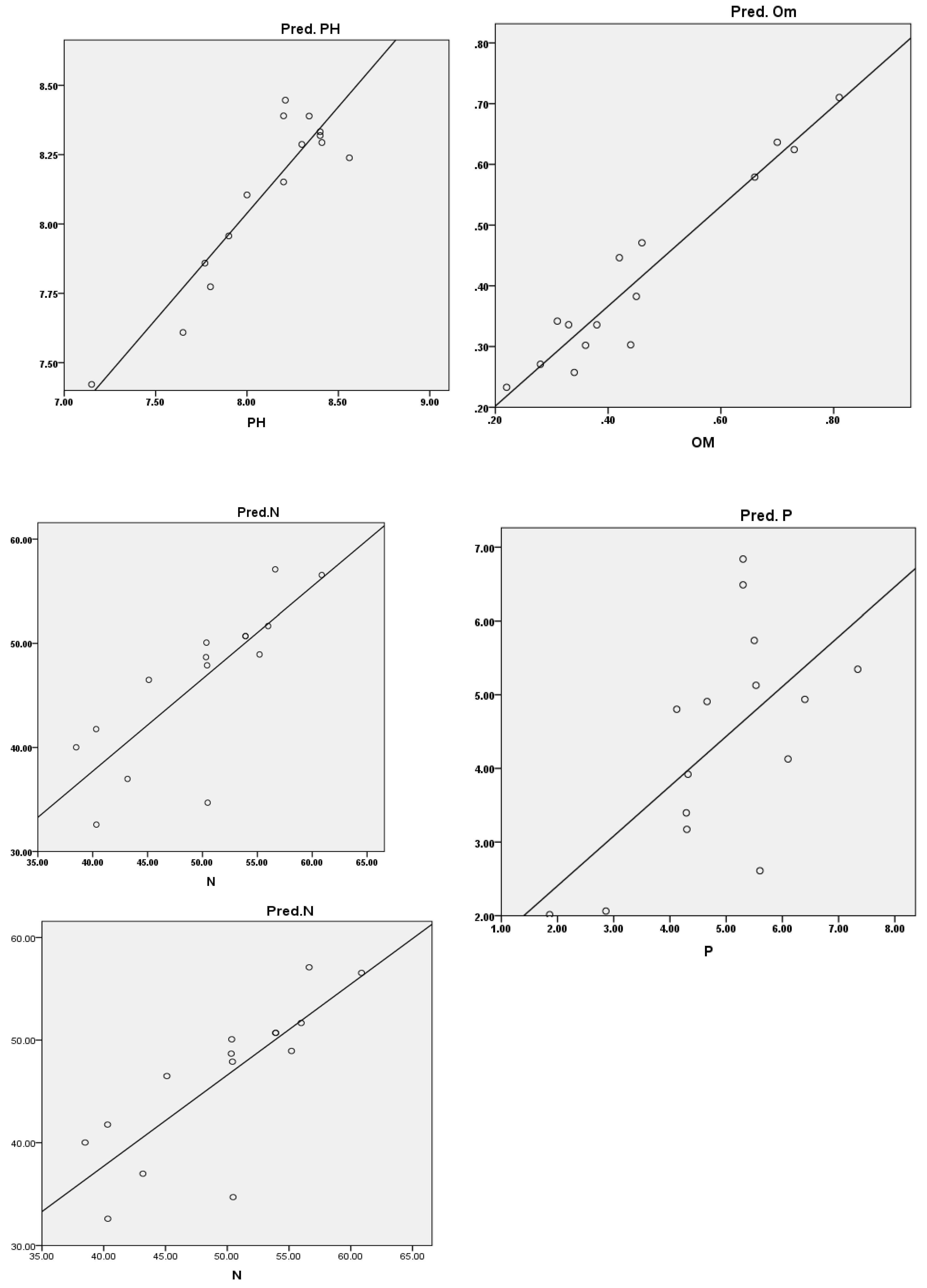
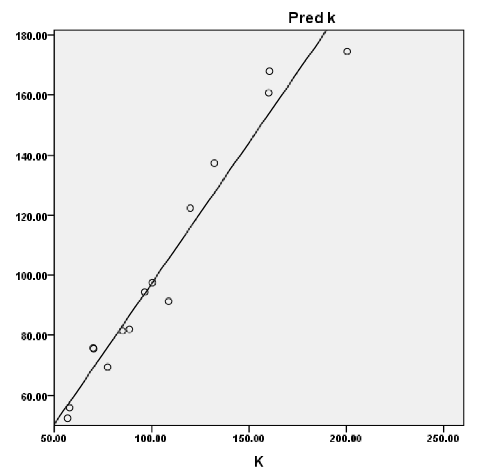
| Selected Parameters | R2 Calibration | Adjusted R | RMSE | NRMSE | R2 Validation |
|---|---|---|---|---|---|
| pH | 0.6 | 0.54 | 0.31 | 0.16 | 0.75 |
| SOM % | 0.7 | 0.65 | 0.11 | 0.14 | 0.82 |
| N (ppm) | 0.55 | 0.52 | 8.70 | 0.1 | 0.74 |
| P (ppm) | 0.6 | 0.60 | 1.53 | 0.01 | 0.50 |
| K (ppm) | 0.92 | 0.91 | 7.89 | 0.04 | 0.97 |
| Statistics | Pred. pH | Pred. SOM | Pred. N | Pred. P | Pred. K |
|---|---|---|---|---|---|
| MAX | 8.54 | 0.71 | 66.15 | 6.84 | 174.59 |
| Mean | 7.90 | 0.38 | 45.47 | 4.18 | 83.37 |
| MIN | 7.28 | 0.05 | 20.31 | 2.01 | 24.13 |
| SD | 0.35 | 0.17 | 9.63 | 1.40 | 30.64 |
| Soil Parameters | Transformation | Trend Type | Model Type | Mean | RMSE | MSE | RMSSE | ASE |
|---|---|---|---|---|---|---|---|---|
| Pred. pH | Box cox | Constant | Spherical | 0 | 0.34 | 0 | 1.01 | 0.3 |
| Pred. SOM | None | Constant | Gaussian | 0 | 0.16 | 0.02 | 0.98 | 0.2 |
| Pred. N | log | None | Gaussian | 5.32 | 14.1 | 0.15 | 0.94 | 28 |
| Pred. P | log | None | Gaussian | 0.01 | 1.24 | 0.02 | 0.95 | 1.4 |
| Pred. K | Normal score | None | Stable | 0.78 | 26.7 | 0.03 | 1.03 | 25 |
| pH | Pred. pH | OM | Pred. OM | N | Pred. N | P | Pred. P | K | Pred. K | |
|---|---|---|---|---|---|---|---|---|---|---|
| pH | 1.00 | 0.753 ** | 0.039 | −0.124 | 0.035 | 0.086 | −0.033 | −0.051 | 0.081 | 0.027 |
| Pred. pH | 1.00 | 0.230 | 0.111 | −0.027 | 0.081 | −0.199 | −0.242 | 0.029 | −0.045 | |
| OM | 1.00 | 0.791 ** | 0.311 * | 0.177 | −0.203 | −0.257 | −0.033 | 0.040 | ||
| Pred. OM | 1.00 | 0.211 | 0.129 | −0.217 | −0.084 | −0.174 | −0.036 | |||
| N | 1.000 | 0.678 ** | −0.057 | −0.096 | −0.047 | 0.062 | ||||
| Pred. N | 1.000 | −0.031 | 0.006 | −0.055 | 0.070 | |||||
| P | 1.000 | 0.456** | −0.271 | −0.165 | ||||||
| Pred. P | 1.000 | −0.223 | −0.275 | |||||||
| K | 1.000 | 0.925 ** | ||||||||
| Pred. K | 1.00 |
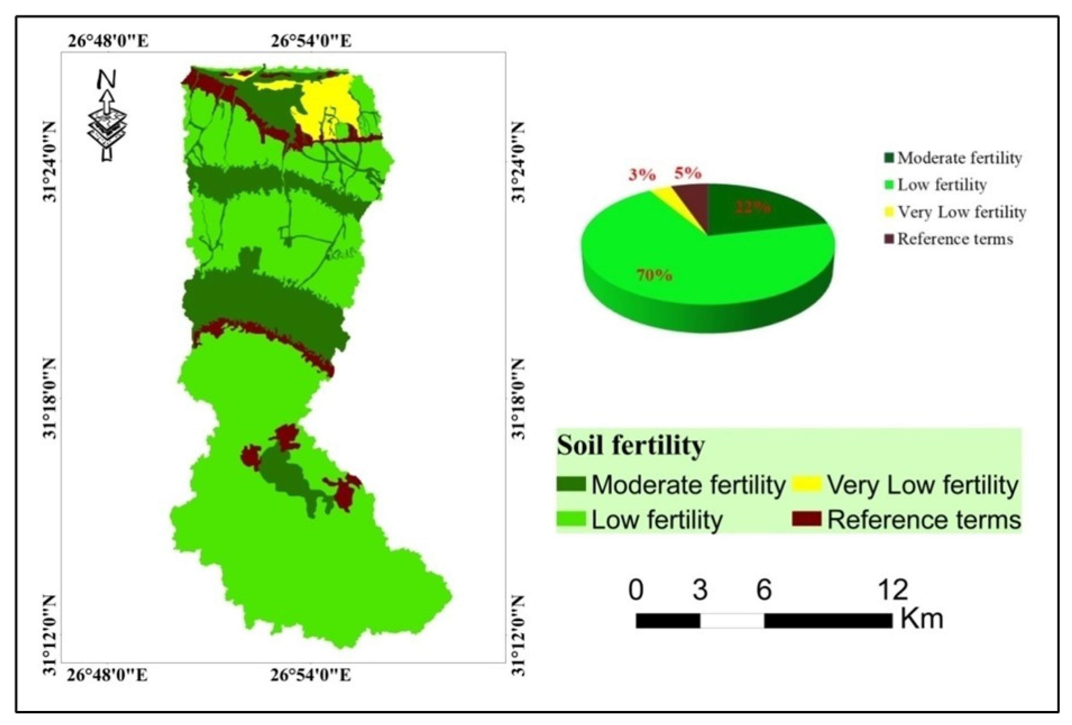
| SFC Classes | Symbol | Area (Hectare) |
|---|---|---|
| Moderate | F3 | 4607.90 |
| Low | F4 | 14,900.21 |
| Very low | F5 | 705.73 |
| References terms | - | 1155.91 |
Publisher’s Note: MDPI stays neutral with regard to jurisdictional claims in published maps and institutional affiliations. |
© 2022 by the authors. Licensee MDPI, Basel, Switzerland. This article is an open access article distributed under the terms and conditions of the Creative Commons Attribution (CC BY) license (https://creativecommons.org/licenses/by/4.0/).
Share and Cite
Shokr, M.S.; Mazrou, Y.S.A.; Abdellatif, M.A.; El Baroudy, A.A.; Mahmoud, E.K.; Saleh, A.M.; Belal, A.A.; Ding, Z. Integration of Geostatistical and Sentinal-2AMultispectral Satellite Image Analysis for Predicting Soil Fertility Condition in Drylands. ISPRS Int. J. Geo-Inf. 2022, 11, 353. https://0-doi-org.brum.beds.ac.uk/10.3390/ijgi11060353
Shokr MS, Mazrou YSA, Abdellatif MA, El Baroudy AA, Mahmoud EK, Saleh AM, Belal AA, Ding Z. Integration of Geostatistical and Sentinal-2AMultispectral Satellite Image Analysis for Predicting Soil Fertility Condition in Drylands. ISPRS International Journal of Geo-Information. 2022; 11(6):353. https://0-doi-org.brum.beds.ac.uk/10.3390/ijgi11060353
Chicago/Turabian StyleShokr, Mohamed S., Yasser S. A. Mazrou, Mostafa A. Abdellatif, Ahmed A. El Baroudy, Esawy K. Mahmoud, Ahmed M. Saleh, Abdelaziz A. Belal, and Zheli Ding. 2022. "Integration of Geostatistical and Sentinal-2AMultispectral Satellite Image Analysis for Predicting Soil Fertility Condition in Drylands" ISPRS International Journal of Geo-Information 11, no. 6: 353. https://0-doi-org.brum.beds.ac.uk/10.3390/ijgi11060353