1. Introduction
The European Common Agriculture Policy (CAP) was set up five decades ago with the goal of ensuring food security, and to support the farmers and agricultural activities of Member States (MS) by implementing a system of agricultural subsidies. The CAP has responded to the economic, environmental and other challenges that Europe has faced at different times by undergoing several reforms. The latest CAP reform, planned for the period after 2020, will see, among other commitments, a reshaping of the updates in the monitoring procedures of CAP measures, including the procedure for control and monitoring system support (Integrated Administration and Control System, IACS) [
1] and the procedure for Control with Remote Sensing (CwRS). The CAP already encourages MS to use Copernicus services (Sentinel data, Copernicus Data and Information Access Service-DIAS) for monitoring the implementation of its measures. However, after 2020 the MS will need to implement some of those updates with reference to the use of common data (Sentinel) to enable better comparability of CAP results achieved by different MS, and to shift from sample inspections to large-scale monitoring [
2].
In each MS, subsidy administration and control are carried out by a National Control and Paying Agency (NCPA) [
3]. During the process of subsidy control, each NCPA must decide on the compliance of farmers’ declaration as well as on the adequacy of agricultural practices on each parcel, and consequently determine whether the management of the agricultural land meets the requirements of the subsidy payment scheme (i.e., the process of CAP measures). Each NCPA is responsible for maintaining the national land parcel identification system (LPIS) and controlling at least 5% of those declarations by performing On-The-Spot checks (OTS, classical/field-based or using remote sensing) and penalizing farmers who submit incorrect information [
3]. OTS checks are performed on a yearly basis, but each year on different sample zones. In Slovenia, the governmental body responsible for these controls is the Agency of the Republic of Slovenia for Agricultural Markets and Rural Development (ARSKTRP), which has been operating since 2000 as a body within the Ministry of Agriculture, Forestry and Food of the Republic of Slovenia (MKGP).
The aim of CwRS is to check the claimed parcels in the office as much as possible using imagery available for the current year [
3]. The primary result of these checks is a control result (diagnosis) at a parcel level. High- and very high-resolution satellite images (i.e., WorldView, SPOT), which the CwRS is currently based on, provide up-to-date location insights and can reduce the number of field visits. However, not all cases of control are solved based on image interpretation. The upcoming reform thus aims to promote the use of satellite data with a special focus on freely available Sentinel-1 and Sentinel-2 time series imagery and DIAS in order to make a substantial reduction in the number of field visits, paying particular attention to a regular monitoring system, and therefore supporting the modernization and simplification of the CAP in the post-2020 timeframe [
1].
The NCPAs can make the right decisions if they possess accurate information on agricultural practices actually being performed, and any major changes that have occurred at the parcel level. This information is now expected to be provided with time series analysis of Sentinel observations. Time series in this respect are defined as a series of consecutive observations, acquired at regular or irregular time intervals [
4]. The Sentinel-1 (S-1) and Sentinel-2 (S-2) are new and powerful sources of radar and optical data for a complete agro-environmental monitoring. In addition to the entire crop or pasture lifecycles, and for monitoring any land change, legal or illegal, the S-1 and S-2 data appear suitable for various application domains (forestry, urban, water, etc.) [
5]. Demonstrating a high capacity for the characterization of environmental phenomena, the S-1 and S-2 data are able to describe trends as well as discrete change events [
4]. Sentinel satellites capture the Earth’s surface with high temporal resolution (i.e., several days), enabling the processes on the Earth’s surface to be studied continuously over a period of time (e.g., throughout the growing season).
Procedures for analyzing and interpreting data that fully integrate the time dimension are a field of intensive research. Assessing the location, extent, type, and frequency of land cover transitions, as well as identifying spatial and temporal patterns of change through interpretation and analysis of frequent land cover information, can provide insights into the underlying processes and drivers of change [
4]. Remote sensing techniques are widely used in agriculture and agronomy. The use of remote sensing is necessary, as the monitoring of agricultural activities faces special problems not often seen in other economic sectors, e.g., agricultural production follows strong seasonal patterns related to the biological lifecycle of crops [
5].
The identification and monitoring of agricultural practices is relevant for a range of ecological, conservation, and political issues [
6]. Grassland in particular is a type of land cover spurring conflict between agriculture and conservation, as the intensification of land use is a major threat to grassland biodiversity. In the context of grassland and rangeland monitoring, remote sensing approaches have been developed for the characterization of grassland type and vegetation change for conservation planning, the mapping of pasture and grassland productivity and the derivation of biophysical properties [
7]. Jakovels et al. [
8] highlight the clear interest from a number of end-users in Latvia for grassland mapping and management practice monitoring solutions. They propose and explore the capability of Sentinel (S-1 radar and S-2 optical) data use and fusion for the assessment of grassland management activities. Grasslands mapping was performed using S-2 temporal data sets, while detection of mowing and ploughing was carried out using S-1 radar data, the latter also being useful during cloudy weather conditions when optical data is not available. Asam et al. [
6] assessed the feasibility of optical RapidEye data to derive leaf area index (LAI) time series and relate them to grassland management in Bavarian alpine uplands. Their analysis is based on exploring LAI variability identified using the standard deviation, where different levels of variability indicate different numbers of mowing events. For an accurate identification of mowing events they emphasize the importance of selection of the time series temporal resolution, and suggest an acquisition frequency of two to three weeks.
The majority of the EU MS use remote sensing to check at least a part of the subsidies for agricultural areas [
9]. Successful demonstration of using S-1 and S-2 images in support of CAP was demonstrated in Denmark. A pilot study completed by DHI GRAS and supported by the Danish Agrifish Agency focused on the integration of S-1 and S-2 data within the field of grass mowing and catch crop monitoring [
10]. The Copernicus Sentinel satellites are also being used to detect and better evaluate the management practices of grasslands in Estonia. The automatic satellite-based grassland mowing detection system has great potential in the context of the CAP, where one of the requirements for subsidy payments is regular mowing of grasslands [
11]. Processes for objective and automated identification of agricultural parcel features concerning the CAP have also been developed for several use cases in Spain and Portugal. Estrada et al. [
9] proposed processing and combining S-2 and LIDAR data for the identification of irrigated areas and landscape elements, while an S-2 based crop identification methodology for the monitoring of the CAP Cross Compliance and Greening obligations was also investigated for a smallholder agricultural zone [
2]. Schmedtmann and Campagnolo [
12] developed a reliable control system of parcel-based crop classification to partially replace Computer-Assisted Photo Interpretation (CAPI) for crop identification, with the overarching goal of reducing control costs and completion time.
An important step towards modernization and simplification of the CAP in the post-2020 timeframe is being made with the implementation of the SEN4CAP project [
1] by the European Space Agency (ESA) in direct collaboration with DG-AGRI, DG-Grow and DG-JRC. The state-of-the-art SEN4CAP project aims at providing the European and national CAP stakeholders with validated algorithms, products and best practices for agriculture monitoring relevant for the management of various CAP measures, e.g., crop diversification, permanent grassland identification, detection of fallow land, catch crops, nitrogen-fixing crops, land abandonment. The main premise of the suggested monitoring of CAP measures is that the declared agricultural parcel state can be tracked using a proposed color-code expressed as ‘traffic lights’ for each payment scheme and the related eligibility conditions. The process of allocating traffic lights consists of assigning an eligibility status to an agricultural parcel. The process is based on a channeling approach: the parcel is monitored until a characteristic manifestation through the applied markers is observed that allows a decision to be made for the application year. The markers are customized observations of signs of plant status in relation to the agricultural activities performed, that can be derived from specific vegetation status indicators (e.g., signs of ploughing, harvesting, grassland mowing, overgrowth) [
1]. The main objective of introducing the described system is to optimize the process of verifying the suitability of land management, in particular reducing the scope of OTS controls and to shift the controls from a sampling pattern scheme (sample inspections) to covering all agricultural areas in the country (large scale monitoring).
Objectives of the Study
The aim of our study is to evaluate the time series approach using S-2 data for the identification of irregularities in the assessment of the agricultural object (parcel)-based management practice. The objective is to identify certain signs of ineligible (inconsistent) areas on permanent meadows and crop fields in one growing season.
Appropriate measures of agricultural policy require only mowing to be carried out on permanent meadows (mowing is also time defined and limited), and that agricultural fields should be ploughed annually or harvested depending on the type of crop planted. Permanent changes in land cover may be the consequence of biotic or abiotic factors, and should be treated in a meaningful manner in the monitoring process. Therefore, when analyzing the detection of irregularities of land use, we are paying particular attention to signs of ploughing or other permanent changes in the land cover in the case of permanent meadows, whereas for crop fields we focus on overgrowing, abandonment or absence of ploughing. In both cases, the observation of the phenomenon is associated with the observation of the continuity in greenness (the unbroken and consistent existence of vegetation).
In the process of crop fields analysis, no attention has been given to the classification of crop types, but instead to land use anomaly detection. The baseline detection of changes was done using the BFAST Monitor method [
13], a methodology for change analysis based on time-series data. This methodology is mostly used to characterize the spatial and temporal changes in forest areas. To date, only a few attempts of its application for agricultural land use changes analysis can be found in the literature [
14]. In our case, BFAST Monitor was used in combination with the analysis of object-based temporal (NDVI) profiles and computation of time series standard deviation as an indication of NDVI variability in one growing season. The complete semi-automatic methodology was developed to obtain results in a relatively fast time and designed in a way that the outputs can serve as a risk parcel warning layer of unjustified use in further control procedures of the national paying agency, ARSKTRP.
A further contribution of this study is the assessment of the suitability of Sentinel-2 data for monitoring fragmented and small-size agricultural land in Slovenia in the context of ongoing reforms within the monitoring CAP area-related measures, considering the spatial, spectral and time resolution of Sentinel-2 observations.
3. Methodology
3.1. Reference Phenology of Observed Agriculture Land in One Growing Season
Observation of the vegetation cycle and knowledge of periodic processes and causes for their occurrence lead to the understanding and detection of anomalies in the growth cycle. For the purpose of our study we examined the reference state and characteristic development of the growth cycle of a permanent meadow and crop field in one growing season, in addition to the visual interpretation of the NDVI vegetation index time series.
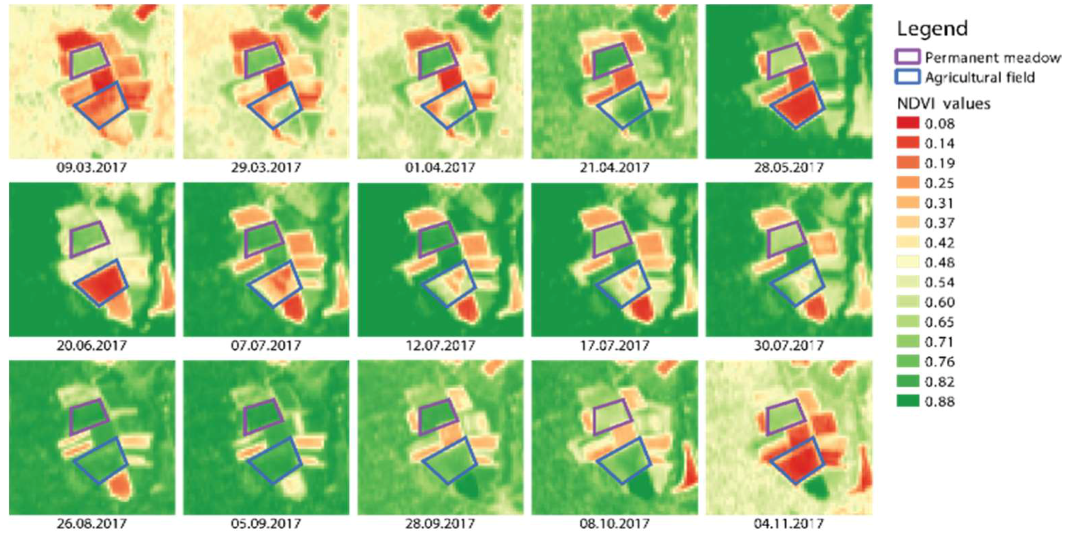
Figure 2 shows examples of a permanent meadow and crop field with the expected development pattern in the 2017 growing season. Dark green shades represent high values of NDVI (>0.5, usually above 0.6), indicating the presence and active growth of vegetation, or vegetation vigor. Red shades visualize lower NDVI values (<0.4) and represent a more substantial lack of vegetation cover. Developmental disturbances in vegetation vigor can be further associated with biotic (e.g., severe drought) or abiotic (e.g., ploughing) factors and triggers. Beige shades (0.4 < NDVI < 0.5) also represent relatively high values of NDVI, and are usually a reflection of young growth or the result of mowing and/or mild drought or of smaller soil outcrops. Both crop types have different temporal patterns due to diverse land use characteristics and the agricultural practices that are applied.
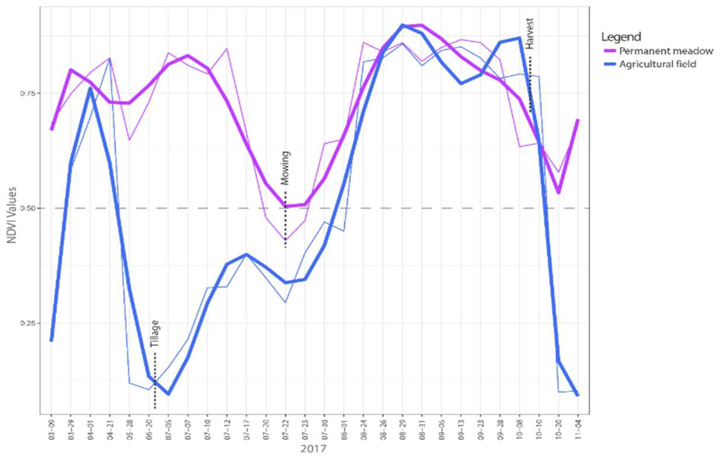
Figure 3 shows that a characteristic permanent meadow maintains high NDVI values throughout the growing season (usually above 0.5). Sign of mowing can be detected by the slight drop of NDVI in the middle of the season. In the case of a crop field, the growth cycle depends on the specific type of the crop grown. Nonetheless, most agricultural crops show a typical pattern of NDVI value consisting of a drop at the beginning of the growing season (indicating tillage), high values in the middle (showing full bloom) and a drop again at the end of the growing season (indicating harvest).
Both growth cycles, visible in
Figure 3, represent a reference (baseline) condition for further analysis of the detection of possible deviations or anomalies on permanent meadows and crop fields in Slovenia and other countries with similar climatic conditions.
3.2. Approach Design
Two important considerations influenced the design of the approach: the selection of mapping unit or unit of phenomena observation, and the short timeframe of available data to conduct an analysis of time series between the years.
Due to the object-oriented interest in agriculture applications in general, and having an agricultural parcel as a base unit in monitoring CAP measures, the use of Geographic Object Based Image Analysis (GEOBIA) [
23] is a good choice. Several GEOBIA-based applications have shown benefits in time-related agriculture applications, especially when crop classification is the main consideration [
4,
24]. GEOBIA typically relies on segmentation algorithms, where image segments are first partitioned from an image into uniform regions, which are later related to meaningful geographic objects [
25] and classified accordingly. However, when a spatial database, such as the Land Parcel Information System (LPIS), or in our case operational national-level administrative layers of agricultural land use (RABA, GERK), are available, this segmentation step is not necessary. Therefore, we do not need to produce meaningful objects from an image using segmentation, and so avoid the possible uncertainties that might occur when creating real world objects from image segments [
26]. Geographical objects in our case are agricultural parcels that form a subset of an already existing spatial information system of high spatial resolution, which represents the physical structure of the landscape. These real-world objects (parcels) provide an up-to-date record of land use in graphical and textual format. The proposed anomaly detection approach is focused on the temporal analysis, seasonal development and specific anomaly identification in parcel objects, thus combining pixel- and object-based analysis.
Important considerations in time series analysis are the length (total time span) and density of the time series dataset (density of time intervals of observations). While some algorithms require uniform spacing between dates to provide calculations and outputs, others can also deal with uneven distributions. However, the main prerequisite for most time series analysis algorithms is a sufficient length of consecutive observations, providing a reference over several years, also referred to as stable history. In this respect, S-2 data with the available observation period (data delivery) since 2015 enables only a short time series dataset. In the timeframe of this study the observation period is only over three growing seasons. This is identified as a weak starting point in providing sufficient and stable reference/history information (two growing seasons with normal development expected) to find the true trends in an observed year (and thus relevant anomaly detection) for the BFAST Monitor algorithm. Due to this poor starting point for anomaly detection performed on short time series analysis, we introduce two additional procedures to control and verify the BFAST Monitor algorithm results.
3.3. Methodolgical Framework
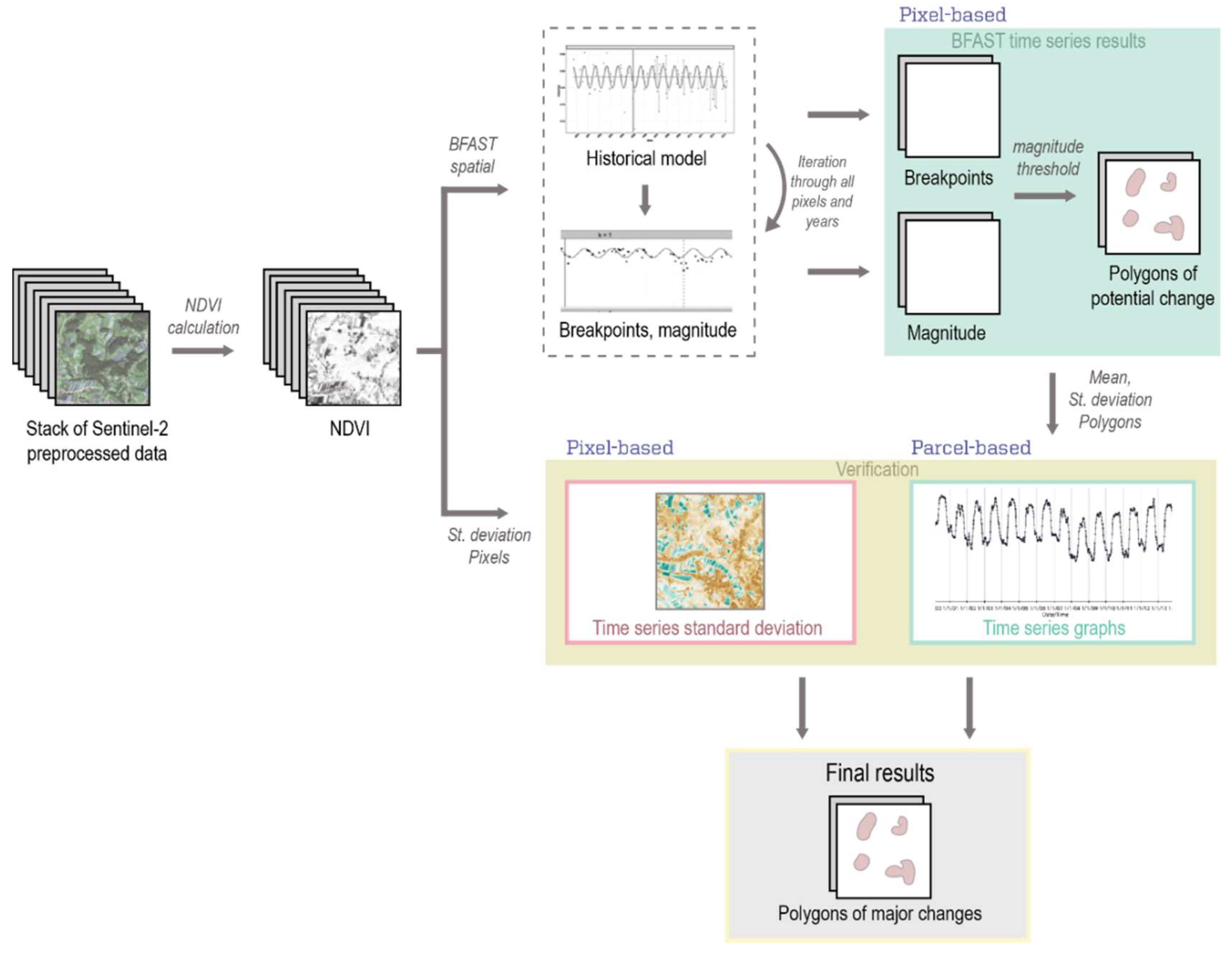
The methodological workflow consists of the following steps: (1) BFAST Monitor time series analysis; (2) time series graphs analysis and (3) time series standard deviation computation. The sequence and connectivity of all steps is presented in the workflow shown in
Figure 4.
Firstly, NDVI layers calculated from pre-processed S-2 data satellite data enter a BFAST Monitor time series analysis. The advantages of analyzing permanent meadows and crop fields with time series are that they can detect dynamic (short and long term) processes, as well as the magnitude of these changes. Each change of values on a particular image indicates possible changes, from which we can get information on both the locations and times of such changes. Secondly, the objects of potential change, which are the results of the automatic BFAST Monitor time series algorithm, present input data for time series graph analysis, consisting of descriptive statistics on the temporal development of objects. Finally, these results are compared with the time series standard deviation output raster, which is calculated using the NDVI time series stack.
In brief, the time series standard deviation method and the BFAST Monitor method focus on time series analysis at the pixel level, while the time series graphs method works on the object level.
The final results of land use type anomalies are selected change objects detected with the BFAST Monitor time series method, which are refined and additionally examined using time series graphs and a standard deviation computation approach. The procedure is semi-automatic and runs separately for permanent meadows and crop fields.
3.3.1. Anomaly Detection with the BFAST Monitor Time Series Approach
To detect changes in permanent meadows and crop fields over time, we performed time series analysis using BFAST Monitor [
13] applying the
bfastSpatial package in the R statistical environment. This methodology was originally developed on Landsat and MODIS data, but can also be applied to other optical satellite data. In our case, the methodology was adapted for time series analysis of S-2 images.
The input data for the BFAST Monitor approach was NDVI time series, calculated from S-2 surface reflectance values at 10 m spatial resolution. These NDVI layers for all dates were stacked into a multi-layer and multi-time raster object on which time series analysis was executed. We assumed that the pixels from the historical period are generally stable and do not contain abrupt changes. Although S-2 images are relatively dense, they are asymmetrically accessible over time (fewer observations in the first years, with the number increasing with time). To facilitate reliable monitoring, the history period needs to be free of disturbances, and thus a stable history needs to be ensured. Though Verbesselt et al. [
13] suggest a stable history period of at least two years to accurately monitor changes (as applied for MODIS data), our history period includes all available observations of roughly two years (2015, 2016), 2015 being the year of irregular data accessibility, as S-2A was launched in June 2015. The complete dataset from 2017 represents monitoring data.
The basic principle of the BFAST Monitor algorithm is the combination of time series decomposition into seasonal, trend, and remainder components with methods for detecting structural changes in both the trend and seasonal components [
27]. The method works by fitting the data on a period defined as stable history and checks the stability of that same model during the period defined as the monitoring period [
28]. Discrepancies between model predictions and data during the monitoring period are estimated, and when the observed data deviate significantly from the model then a break or a time of change in a decimal year is detected. The differences between the expected and observed (actual) values during the monitoring period are also shown in the form of positive or negative magnitudes of changes. We predicted that the correlation between magnitude and irregular use of permanent meadows is shown in negative values (the drop of NDVI as a cause of tillage or bare soils outbreaks), whereas crop field changes that indicate possible overgrowing or abandonment are shown with positive magnitude values (the increase of NDVI as a cause of overgrowing, lack of crop treatment practices).
As the BFAST magnitude results provide magnitude intensity values, these have to be ranked in order to select those showing a potential land use anomaly. Based on the severity of changes for candidate anomalies only objects with pixel values under or over two empirically determined thresholds were included for subsequent analysis. Thus, objects containing areas of pixels with negative magnitude of changes lower than −0.22 were chosen for permanent meadows, and objects containing pixels with positive magnitude over 0.4 were chosen for crop fields.
The results of BFAST Monitor can be presented on a single pixel (point) in the form of time graphs, or on a raster (area). Mapping the results enables a detailed (due to pixel-based calculations) and clear visual insight into possible changes in the study area under consideration. However, raster processing is much more complicated and time consuming than calculating time series on an individual pixel. A parallelized approach was applied to accelerate the computational time of raster time series analysis, drastically speeding up the processing (instead of taking five hours the results were obtained roughly in 10 min).
3.3.2. Time Series Graphs
The time series graphs approach is based on the analysis of NDVI temporal development curve for each individual object of permanent meadow or crop field. Basic descriptive statistics (mean, standard deviation) are calculated for each candidate object obtained from the BFAST Monitor algorithm. As already mentioned, a parcel object represents the basic unit of observation for this method. Thus, the mean and standard deviation were calculated for each object on each satellite image of the time series. Temporal graphs provide an insight into the growth cycle of the analyzed vegetation type during the growing season (or longer), and thus enable effective identification of deviations from the expected trend of observed phenomena within a growing cycle (see
Figure 2). What needs to be defined is thus the threshold value that enables effective distinction between the active vegetation growth and non-vegetation. The empirically selected value was set to 0.4, taking into consideration the findings in
Section 3.1 (
Figure 3).
All the statistical calculations are averaged per geographical object (parcel), thus the time series graph approach deals well with radiometric noise persisting between satellite observations. As such it serves as a complementary measure of anomaly detection at the object level, being less sensitive to direct NDVI readings, but still able to intercept changes.
This approach complements the BFAST time series methodology, described in the previous chapter, and constitutes an additional control of candidate anomaly objects. If confirmed by both methods, such a change object is labeled as a land use anomaly.
3.3.3. Time Series Standard Deviation
Compared to the time series analysis based on detection of trends and breaks, in this simple approach we calculate the standard deviation for the individual pixel over the entire NDVI time series in one growing season. The final result is a raster layer of the standard deviation values over the anticipated period. Few agricultural activities at an object level result in a low standard deviation value over a growing season, while changes and leaps in NDVI values (potentially due to changes between soils covered with vegetation and bare soils) significantly increase the standard deviation value for the growing season.
The time series standard deviation layer provides informative data for the pixel variability over time. Low variability is expected on permanent grassland pixels if grassland was present and only grassland related activities such as mowing were implemented. On the other hand, high variability is expected on crop fields if appropriately managed (plant growth, harvest, new growth) while low variability could be associated with abandonment and thus irregularity of crop field land use.
The time series standard deviation is an accumulative measure and as such additionally informs the verification of possible areas with unjustified land use in the growing season (i.e., in comparison with the official farmers’ declarations).
4. Results and Validation
The results of our approach are shown in
Figure 5 to Figure 9. At the same time, we also provide an analysis of their reliability and relevance, crucial for the assessment of the proposed workflow. This is followed by a validation section, giving the results of methodological correspondence and cross-comparison, as well as of the validation with independent data from official land use controls of the national paying agency (ARSKTRP).
4.1. Results and Workflow Assessment
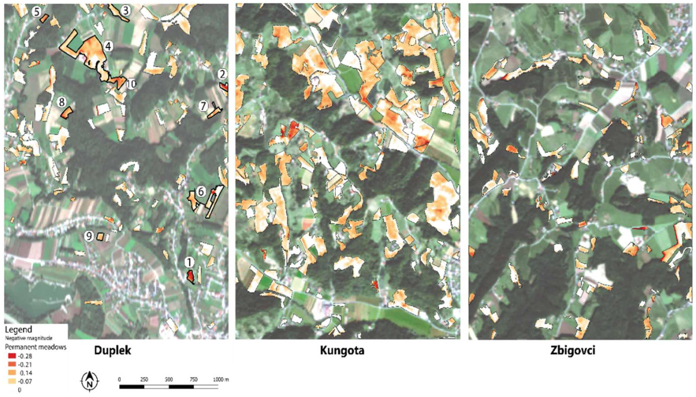
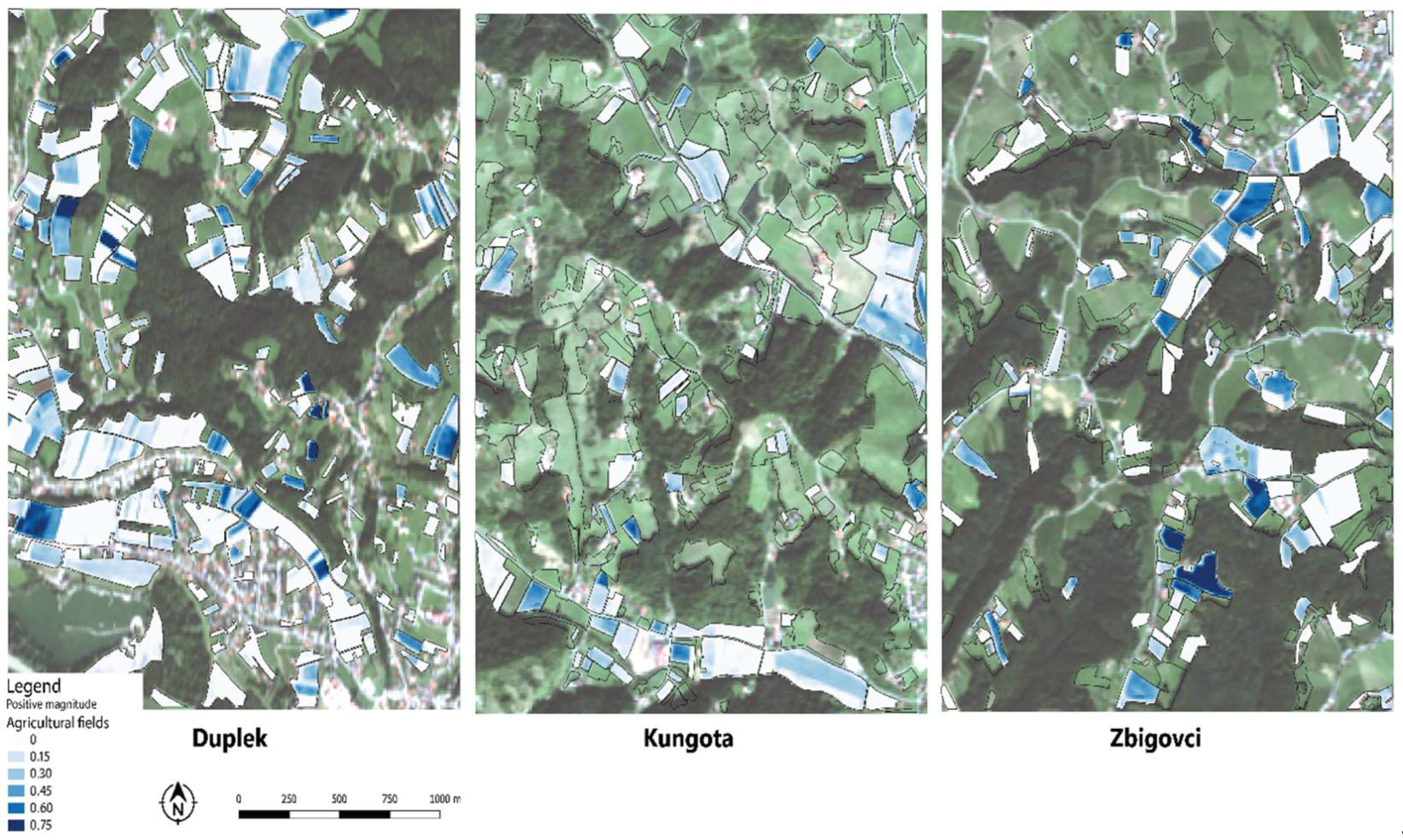
Firstly, our results show the detected magnitudes of change for each of the analyzed land use types obtained from the BFAST Monitor analysis of trends and deviations. It is noticeable that both positive and negative changes are present over all study areas and on both land use types under consideration. For the purpose of detecting irregularities, we focused only on negative changes in the case of permanent meadows (displayed in red color scale,
Figure 5) and positive changes in the case of crop fields (displayed in blue color scale,
Figure 6). The empirically determined thresholds are applied to label objects with a severe level of change. A sample of 10 thresholded objects with the highest magnitudes is highlighted in
Figure 5 (left, Duplek area). The selected objects are further used to display the results of other methods and cross-compare their performances, as well as for sample visualization of the results in this paper.
In order to understand the BFAST Monitor magnitude results in more detail, extreme values of changes in the NDVI were additionally considered. This information is crucial to decide the reliability of the automatic outputs. Extreme values in the NDVI changes can represent either an actual drop in values or apparent or even false changes. False changes were recognized mainly as the consequence of an insufficient number of reference observations (unstable historical period), which can lead to the generation of wrong trends. In general, inaccurate or apparent changes may also be present despite careful data preprocessing (e.g., elimination but not exclusion of geometric and atmospheric errors and noise reduction), and might also be the consequence of an erroneous cloud mask. This means that areas under undetected small clouds and cloud shadows might be present on the images, and thus might have different spectral values than the actual values on the surface. Since we used only cloudless S-2 images (as ensured by double-checking using the STORM processing atmospheric mask and visual inspection), the low NDVI values are considered as reliable information about any irregularities, but the short historical period might still present an issue. This examination confirms that short time series are highly sensitive to any differences between the years taken as the learning or historic period, and if an diversity exists then the trend calculation returns unstable results, which are very likely incorrect trend predictions. This confirms that when a time series is short (i.e., a few years only, as is the case with S-2 data) or the historic years summarize different meteorological conditions (e.g., agriculture drought year, normal year) it is necessary to test the BFAST Monitor time series analysis results additionally, using statistical approaches as a supplement. We proposed two verification measures, i.e., time series graphs and/or time series standard deviations in the further steps, which can provide additional information in the case of insufficient data.
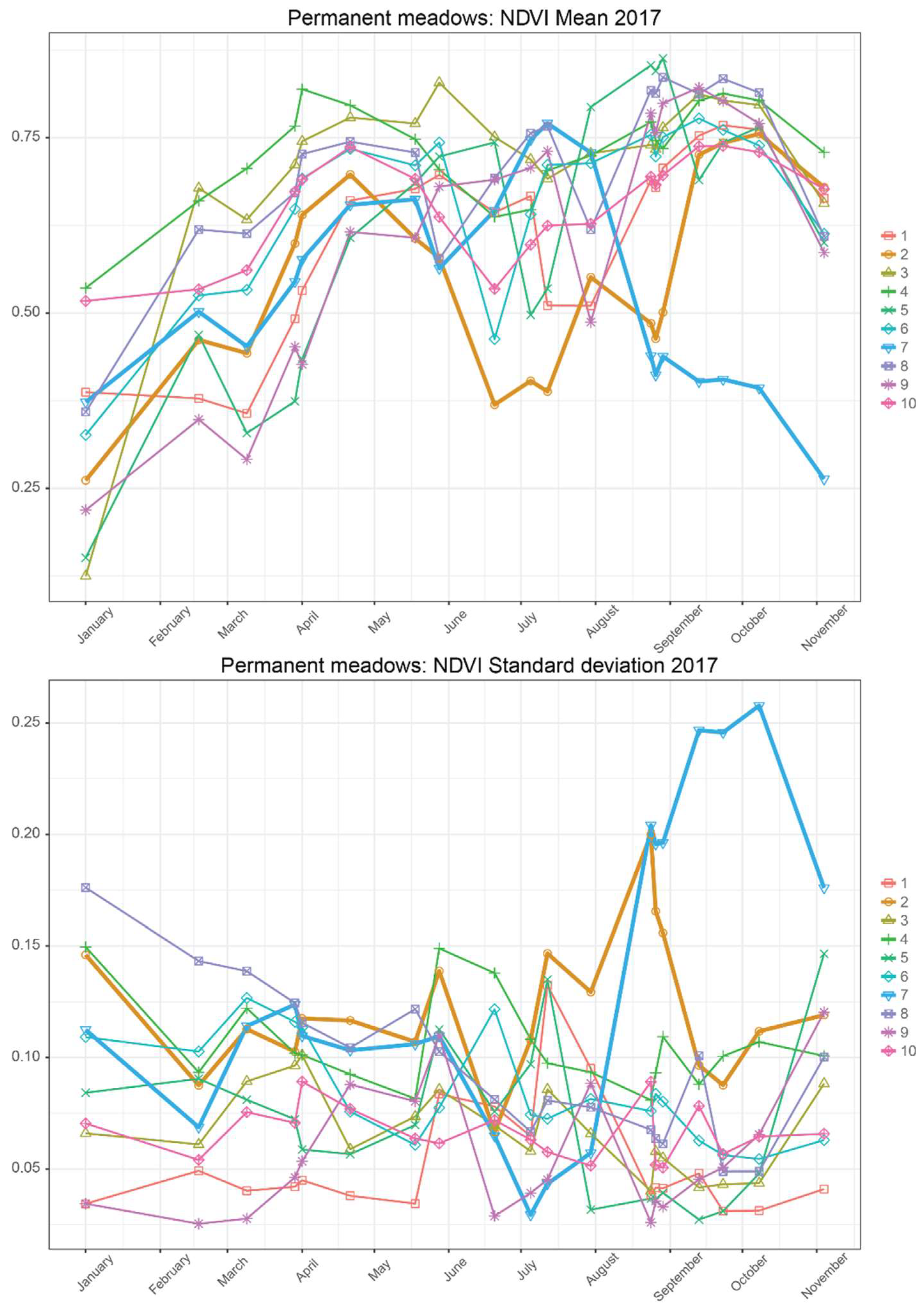
Moving to the results of time series graphs, it must be re-emphasized that the mean and standard deviation are calculated based on the whole object (from all pixels in the object). This means the NDVI values can still be high despite the presence of irregularities (ineligible, non-compliant use) inside the object. The mean NDVI development curve for the 10 analyzed permanent meadows objects (from
Figure 5), which could represent irregularities in the expected annual phenology (i.e., permanent greenness), displayed using temporal graphs is shown for illustration in
Figure 7. In more detail, see, for example, object no. 7 that still exhibits high and thus non-suspect NDVI mean values close to 0.4 in August-October in the top figure, while its standard deviation trajectory points to a much more pronounced deviation from the other objects and expected temporal behavior of permanent meadows under the CAP allowable management regime, in the bottom figure. Specifically, this case suggests that the complementary consideration of both measures (mean and standard deviation) is beneficial and a necessary control measure in our anomaly detection workflow. Our results suggest that the temporal graph of standard deviation values is a useful measure for deviation observation, and additionally allows for deviation detection in the object parts.
As outlined above, it is crucial to consider different measures of anomaly detection, in order to build a framework that produces reliable results. The rationale behind our approach is that attempting to automatically define land use anomalies will lead to poor accuracies if (1) the context for the anomaly recognition is not well defined, and (2) algorithm performance is not systematically examined. Thus, as a supplementary verification, we introduce a comparison between two consecutive years that may indicate whether such anomaly situation on the agricultural parcel was present during the previous year. For the illustration of such a measure for anomaly candidate selection, a deviation from the reference growth cycle of permanent meadows is noted in
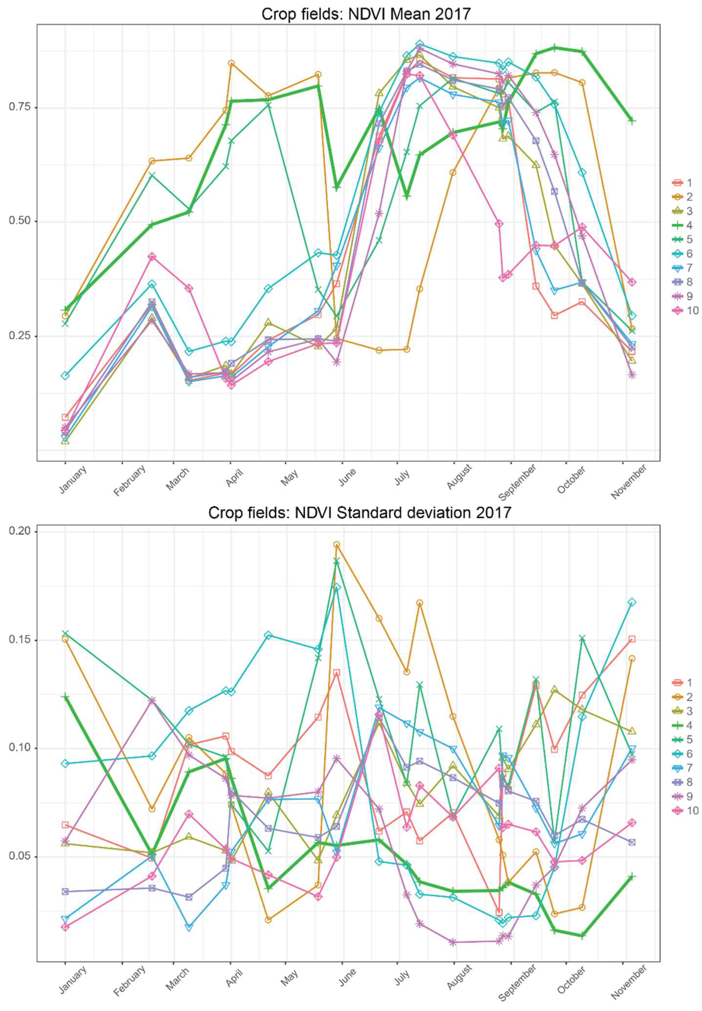
Figure 7 in the case of objects no. 2 and no. 7 (darker yellow and blue), and in
Figure 8 in the case of crop field object no. 4 (light green). From
Figure 7 and
Figure 8 we can observe that for permanent meadows the occurrence of a drop in mean NDVI resembles irregularities, which are represented in high standard deviations, whereas for crop fields we search for anomalies with a high mean NDVI and low standard deviation in time series graphs.
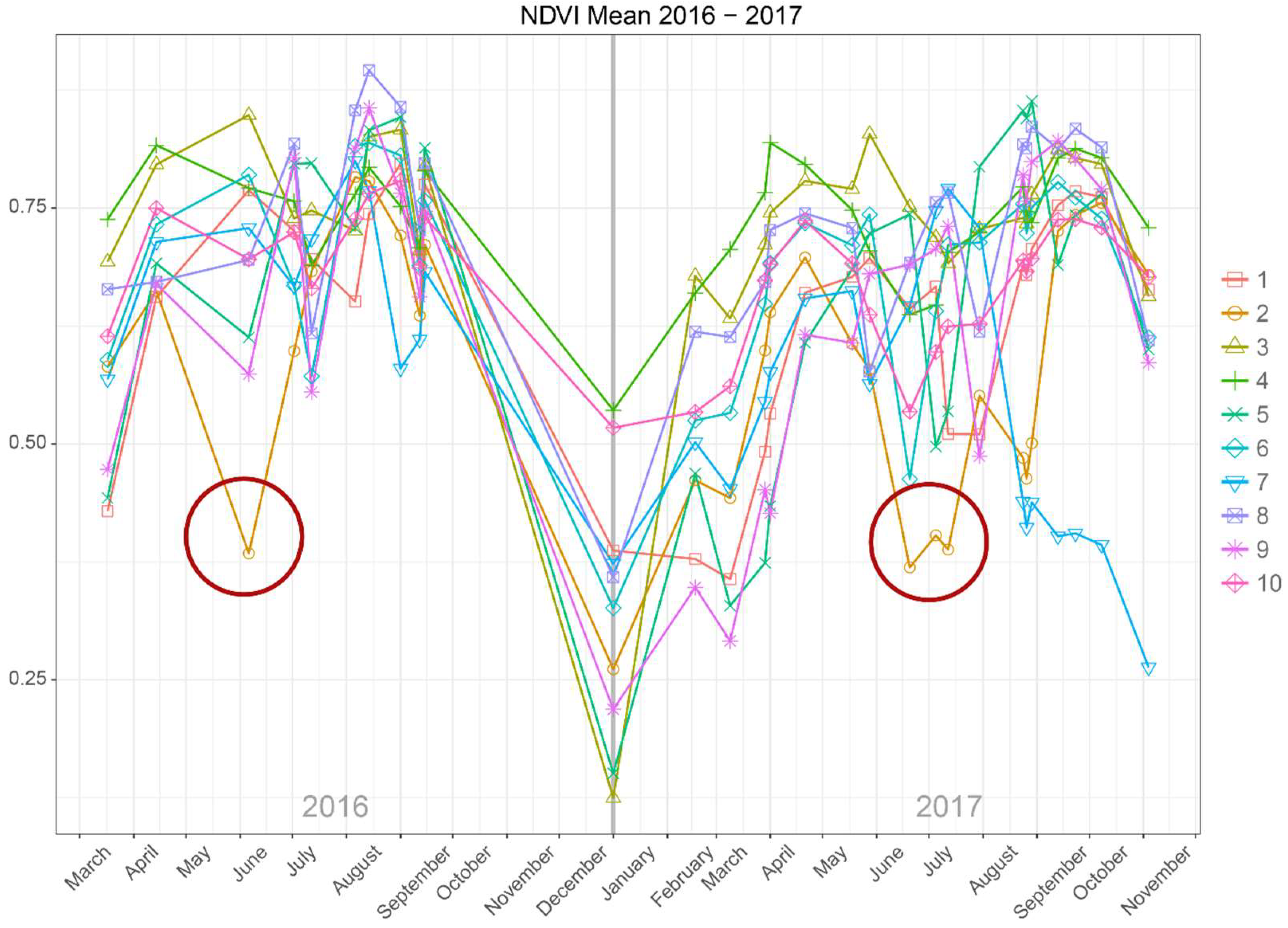
Objects of interest were later inspected beyond the given growing season, and the results of this comparison are given for objects of permanent meadows in
Figure 9. Here we are interested in the deviations of the mean values of the NDVI temporal graph and in drops below the 0.4 threshold (an indicator of potential land use anomaly candidates in 2017), and also if it shows similar deviations as in the previous growing season (2016).
The results of the inter annual comparison show that for object no. 7 (
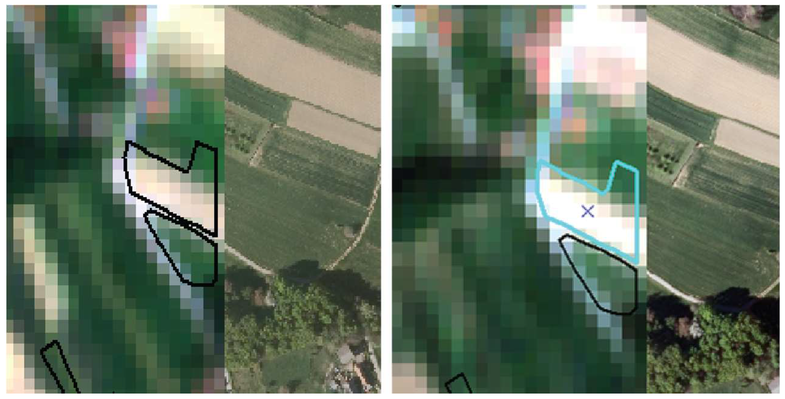
Figure 9) no remarkable deviations from the expected trajectory can be observed in the 2016 growing season. In contrast, if we focus on the development curve of object no. 2 (dark yellow line), remarkable declines (marked by two red circles) in the value of NDVI in both the 2016 and 2017 growing seasons are clearly noticeable. Nevertheless, both problematic objects’ mean NDVI values are within the established threshold value, which separates active vegetation areas from inactive ones (bare ground, soil or built-up area). Finally, additional confirmation was obtained through visual interpretation of S-2 imagery (
Figure 10), which revealed characteristic bright surfaces during the problematic dates. This case is very likely to represent a disparity between the declared use (permanent meadow) and the actual state of land in nature (non-vegetated ground).
Using the results of the inter annual comparison it was possible to confirm that the two objects that were limiting the mean NDVI criteria for anomaly detection truly contain pixels with obvious changes. Our results thus suggest that interannual information on their significant differences from the expected seasonal trajectory can be defined and included in the verification workflow process.
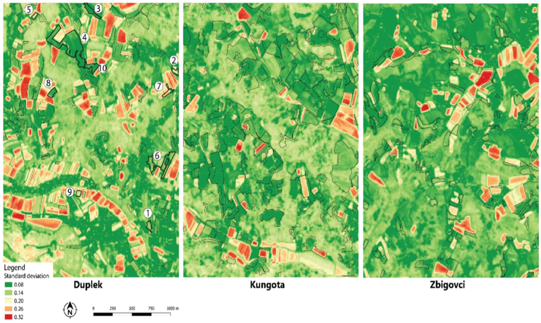
To explore the potential contribution of yet another simply derived measure, we examined the results of the third proposed method—the time series standard deviation. The layer of computed pixel-based standard deviation values (
Figure 11) obtained at the end of the growing season represents a simple descriptive statistic—the variability in NDVI values as accumulated over the growing season. The result is thus a single raster layer indicating variability intensity. As such the layer enables an efficient differentiation between intensively managed areas (ploughed crop fields or other abiotic changes implying ineligible use, shown in red with high standard deviation values) and less intensively managed areas (permanent meadows and other vegetation, shown in green tones). As expected, the results confirm that this method does not provide information on the time that such changes occurred within one growing season, although being pixel-based it can support a clear spatial indication of changes within objects.
Our results suggest that the time series standard deviation layer provides useful information for the detection of deviations in parts of the object. It is thus recommended to include this measure in the workflow to confirm the changes indicated with the time series graph method.
4.2. Validation of Results
Using the selected approaches for the S-2 images time series analysis, anomalies in the 2017 growing season were detected. All objects containing potential changes obtained with the semi-automatic time series approach and magnitude determination were inspected with the combination of the time series graphs (mean, standard deviation development), and visual checks of objects on S-2 imagery time series and the time series standard deviation raster layer. The main objective of this multi-method cross-comparison was to obtain an insight into the overall quality of the results, the anomaly detection capacity and completeness level, and to identify the circumstances in which possible miss-detections might occur. Based on the results we can introduce all the necessary logic checks to advance from a semi-automatic to a fully automatic workflow.
The correctness of the obtained results (detected land use anomalies) for permanent meadows using the proposed combined approach was verified by the inventory of the official land use controls of the national paying agency, ARSKTRP. Due to time and personnel constraints this validation was done only for the permanent meadows land use type. In total, nine objects of detected irregular use were considered for validation by the national paying agency personnel. They examined the proposed anomalous objects and compared them with the farmers’ declarations and other information collected as part of the land use control process. They returned the information on their (in)correctness in the form of an attribute table of inspected objects (true/false). The inspections confirmed that our approach gives highly reliable results as all the signs of change were associated with real events or reasons causing land use change.
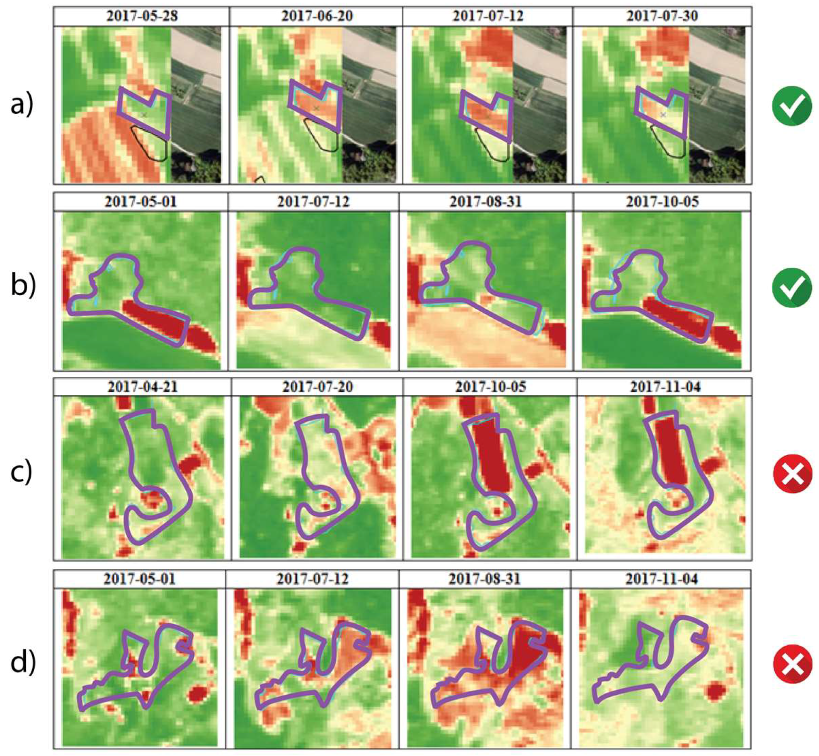
We prepared
Figure 12 for clearer presentation of the results obtained from this verification. The figure gives, on one side, a visual overview of the perceived deviations from the expected phenology of a permanent meadow and, on the other, the anomaly interpretation within the context of an ineligible land use control process from the side of the national paying agency, using four objects confirmed by this agency.
For example,
Figure 12a depicts an inconsistency in permanent meadow land use, as areas of both permanent meadow and crop field are present. But as the land owner reported the land use for this particular parcel as half permanent meadow and half crop field, this is not an irregularity in the context of recognizing anomalies in terms of the land use for the subsidy process. This only indicates the discrepancy between the database used by the national paying agency (ARSKTRP) and the RABA database, which was used to obtain objects of interest for the analysis. A similar example can be seen in
Figure 12b, where the use of a permanent meadow was declared only for half of the object.
Figure 12c,d show inconsistencies in the land use, but, unlike in the first two cases, the national paying agency confirmed irregular use in both cases (the use of crop fields instead of permanent meadows).
On the other hand, verification of the results on candidate anomalies in crop fields (abandoned and overgrown fields) was only possible by means of visual inspection of S-2 imagery, time series graphs and time series standard deviation. The crop field phenological patterns are much more complex and might vary from year to year because of using a rotational system, changes in agricultural practices and/or varying meteorological conditions [
29]. Due to this variability, a stable history which is needed for relevant time series analysis and anomaly detection using BFAST Monitor algorithm cannot be obtained in the case of crop field land use. Therefore, in the case of crop field time series analysis it is important to observe the development of field characteristics on a multi-year basis, taking into consideration possible differences in planted crops, their rotation between different years and corresponding management regime (e.g., fallow land). When abandonment or overgrowth is observed in this respect, we expect similar vegetative development to the permanent meadow land use type, i.e., without sudden and major changes (due to ploughing or harvesting) and thus focus on tracing the continuous greenness.
For the assessment of abandonment or overgrowth as anomalies at crop fields we conclude that the use of a combined approach of times series graphs and time series standard deviation would constitute a sufficient workflow and could outperform the BFAST Monitor algorithm. BFAST Monitor does not guarantee that the trend can be reliably defined in complex and annually changing regimes of crop fields, the situation typically prevailing in Slovenia.
The findings for the proposed methodology (given through examples in the previous sections) are valid for all three study areas and both anomaly detection cases (permanent meadows and crop fields workflows). Moreover, the level of the quality of the obtained results (quality of assignments, completeness and reliability) is comparable across study areas.
4.3. Cross-Comparison of Methods
To compare the adapted time series methods used in this work, we matched their scale and deviations of values for the 10 selected example permanent meadows in the Duplek study area. As noted, these 10 meadows represent areas with high negative changes detected from trends using the BFAST method. Changes do not always occur over the whole object and may be high only in certain parts of the objects, but are still included in the analysis (see meadow anomaly images in
Table 2).
Table 2 shows that mean negative values of magnitude range between −0.05 and −0.2. To see if these objects of negative magnitudes really contain low NDVI values, we calculated the minimum NDVI value for each of the objects and assigned the time when this drop appears using the time series graph method (pixel-based statistics). As seen from the
Table 2, objects 2 and 7 contain the lowest NDVI values (both are under 0,4). Similarly, the mean NDVI standard deviation, calculated on object-based units (meadow parcels), is the highest for both of these objects (over 0.15). Values that deviate from normal behavior using all three methods indicate irregularities present in the analyzed time period.
This comparison of methods is based on the deviation of statistical values relative to their average values. The results highlight that their trend of boundary values coincides, especially for the time series graph (method 2) and time series standard deviation method (method 3), where the most extreme values are exactly for objects for which we suspect possible irregularities. The BFAST Monitor results can give more diverse results, again due to varied values in some parts of the analyzed meadow objects.
5. Discussion
5.1. Reliability and Stability
Reliability and stability are the two main parameters to evaluate the results of the anomaly detection workflow.
Reliability indicates the level of membership and completeness of the assigned anomaly objects for a certain land use anomaly. The higher the membership, the better the completeness and the greater the reliability. However, full assessment of reliability is only possible with the support of the actual land use information for a given growing season. Farmers’ declarations on the actual land use obtained within the subsidy granting process would be an option for such an estimation, although this data is not publicly accessible. Nevertheless, the case of permanent meadows (where evaluation was done on a sample of assigned anomalous objects by the national paying agency ARSKTRP) affirmed that the reliability is high for most assignations, with clear arguments for the presence of all detected changes in permanent meadow objects (see
Figure 11). On the other hand, the reliability estimation for anomaly detection in the crop field land use (i.e., signs of field abandonment) was not carried out due to the inaccessibility of validation data during the study timeframe.
Stability estimates the robustness and transferability of the proposed anomaly detection workflow. We believe that the workflow is well conceptualized for the detection of specific land use anomalies under a certain land use management regime (non-compliant land use), and in this regard is robust and allows for geographic transferability. Minor parameter adaptations might be needed as anomaly assignments are currently based on the thresholding conditions. However, in the case of observing other signs of anomalies that are also important under CAP monitoring measures, workflow transferability might be low. More specifically, both of the proposed workflows only take into account anomalies that are associated with continuous greenness (e.g., signs of ploughing in the permanent meadows, sign of vegetation overgrowth and lack of agricultural activities in the crop fields), which can be well defined and described with vegetation monitoring indicators and with consideration of observed phenomenon time constraints (expected field management regime), and thus controlled for within the specifications of the workflow logic.
5.2. Relevance to Environmental CAP Schemes, Monitoring CAP Measures, Expandability
Identification and monitoring of plant growth on agricultural land through the entire growing season using time series enables users to identify (1) growth development curves for different crop types (and thus recognize particular crop types), as well as (2) different agrotechnical management activities (mowing, plowing, harvesting). Since both characteristics are defined with a specific crop type related time interval, such changes on agricultural land can be identified and monitored. Using Sentinel time series and customized anomaly detection workflows are considered a promising combination to monitor CAP-related measures. In particular, the measures that can be checked in this way are those where the plant development needs to be monitored over time, and where the specific time regime is foreseen and compulsory throughout the growing season.
Customized anomaly detection workflows can be designed to monitor CAP measures and operations for the forthcoming post-2020 reform, i.e., the CAP area-related measures. The customized anomaly detection workflow presented in this study for certain non-compliant land uses on permanent grasslands and crop fields offers numerous possibilities for extension, although a higher complexity may lead to lower anomaly detection rates in selected land use types.
One possible extension is the inclusion of additional anomaly types for additional land uses (e.g., habitats). Currently, our approach identifies anomalies in land use that were recognized as the most relevant issues for the national paying agency ARSKTRP within the subsidy granting process: agricultural inactivity on parcels declared as crop fields and inappropriate agricultural treatment of permanent meadows where only mowing is allowed. Our approach is thus designed to identify anomalies in vegetation greenness as exhibited through the entire growing season. At the moment, this and the scope and sparse context are limitations of the algorithm. With the extension of the current anomaly workflow to other ineligibilities in land use or to other agricultural land use types, new considerations taking into account precise definitions of allowable (compliant) practices within permissible time regimes for the considered land use type could be introduced. In this way, different customized anomaly detection workflows might detect specific ineligibilities in particular land use types even more precisely.
In order to develop an all-inclusive anomaly workflow, new decisions (on anomaly measurements) have to be defined. These decisions would enable the workflow to deal with many different compliant regimes such as: greening of arable land, where arable land should be covered with winter greenery between 15 November and 15 February, an unbroken green belt of grass where mowing or grazing is not allowed between 15 July and 15 September in the operation “grassland habitat of butterflies”, or where mowing and grazing is not allowed before 1 August in the operation “habitats of moist extensive meadows”, to list a few of possible measures and operations of interest for monitoring within CAP-related control measures. Nevertheless, the performance and ability of individual, customized or complex anomaly detection workflows first requires a precise definition to be aligned with the context of supporting CAP processes, as well as the assessment of the workflow suitability, reliability and usefulness according to the type of agricultural policy measure and associated non-compliant land use.
Another limitation of the current study is that anomalies are observed only on NDVI-based vegetation observations. An important possible extension of our existing approach is the implementation of complementary information on vegetation and soil conditions. The performance and ability of other vegetation indices or biophysical parameters to detect certain land use anomalies could be tested and meaningfully introduced. A precise study on the influence of different vegetation indicators might reveal important relationships that could bring more confidence and introduce weights to anomaly/change assignments.
5.3. Anomaly Detection Workflow Considerations and Direction of Improvements
The analysis of satellite image time series aids in understanding and recognition of spatial and temporal patterns of change, as well as their location, extent, type, frequency, magnitude, the direction of change and trends. The BFAST approach presented in this study enables the detection of anomalies on permanent meadow and crop field objects based on a comparatively short time series of S-2 satellite data. This implies that the whole history period, defined from 2015 to 2016, is identified as relatively stable. Although time series graphs and time series standard deviation approaches showed that the BFAST Monitor approach overestimated the segments of land use anomalies, no false positives were detected. In this context, we can predict better and more reliable results using the presented BFAST approach in the coming years, when temporally denser S-2 images will be available and consequently a more stable history period will be possible to achieve. Still to consider is the fact that monitoring agricultural land use on a single vegetation index can have its limitations, as the methodology might not be satisfactory to capture the complex seasonality of heterogeneous land use, especially in the case of permanent meadows. Crop rotation over the years is also a major challenge for analyzing anomalies with time series, since annual crop differences associated with crop rotation system can disturb the seasonal or trend observation (underlying the BFAST model components).
Compared to the BFAST approach, the time series standard deviation output does not require data from previous growing seasons. However, despite its computational simplicity the standard deviation approach provides an insight into parcels’ phenological variability and enables the identification of abrupt changes.
Only optical satellite data were used as the primary source for analysis in this study. When relying only on optical imagery it is important to ensure high time series quality, as this can impact the robustness of the method besides the geometry, size and homogeneity of the observed object (parcel). Concerning the temporal aspect, we estimate that at least one cloudless image should be available per three or four weeks in order to reliably identify non-compliant use.
The experimental results in this study were obtained using a semi-automatic approach, which means that inputs (and especially thresholds) are needed from an experienced user. To improve our workflow, we plan to develop the methodological part into an automatic anomaly detection procedure, where thresholds throughout the workflow will be selected using appropriate multi-level thresholding techniques.
5.4. Agricultural Policy Area-Related Measures and Sentinel Data for the Monitoring of Cap Measures in the Agricultural Landscape in Slovenia
The CAP post-2020 reform will reshape the agricultural land use control procedures, mainly by fostering the use of Sentinel data and encouraging procedures based on regular monitoring. This will have an impact on everyday practice for monitoring a variety of CAP measures. At the moment, bodies responsible for CAP-related reporting seek information on the adequacy of Sentinel data for monitoring agricultural land in Slovenia in accordance with the expected CAP reform. Three considerations are identified as the most pressing: (1) how to respond to the replacement of the selected risk field-based monitoring approach with an all-inclusive one within the process of control under subsidy granting; (2) how can measures regarding green payments, agri-environmental-climate payments, organic farming, less-favored areas for agricultural production and coupled support schemes be monitored appropriately and at sufficient detail with Sentinel data; and (3) how could area-related agricultural policy measures, associated with the diverse size of the agricultural land from 25 m to 5 ha, be accomplished under updates referring to the usage of common data.
There is a substantial difference in the extent and structure of agricultural land among the MS. Comparatively small, fragmented and often narrow agricultural land prevails in Slovenia. Thus, an assessment of suitability of Sentinel data for monitoring CAP area-related measures in Slovenia is important. Concerning the minimum mapping unit (MMU), a study by Devos et al. [
1]) suggested that in order to derive meaningful information for the Earth observation products supporting CAP procedures, the basic unit of analysis should contain at least 20 to 30 pixels. However, the selected MMU of 0.1 ha (10 pixels) in our study resulted in a reliable output. In the case of small parcel objects, it is also advisable to apply a buffer and take into consideration only pure pixels [
12]. Similarly, in the case of narrow parcels, it is necessary to ensure that only representative pixels are considered. However, the usability of S-2 data might be limited in a longitudinal highly fragmented agricultural landscape (where MMU of 0.1 ha pure pixels is not reached). Agricultural land parcels in Slovenia will need to be classified according to size, shape and geographical position, and agricultural areas that are appropriate for monitoring with S-2 under CAP-related measures will need to be defined. Thus, depending on the different geographical and agricultural regions of Slovenia, all of the combinations of Sentinel data, data processing methodologies, as well as monitoring of selected CAP measures should be jointly considered.
The results of this study using S-2 time series have the potential to assist in agricultural parcel monitoring and therefore support decision making on farmers’ compliance on a through-the-year basis. The complete semi-automatic land use anomaly detection workflow was developed to obtain results in a relatively fast time and designed in a way that output can be directly used as a risk parcel warning layer of unjustified (non-compliant) use in further control procedures by the national paying agency, ARSKTRP.
It seems it is not a trivial task to provide reliable information on changes in land use when analysis is based on data from the last three years. Much longer time series are required, especially in the case of crop fields, where sparse historic and no reference data are accessible. Obtaining non-compliant use from S-2 data can therefore be assumed only generally, and the results of the proposed anomaly detection workflow are currently a demonstration of possible approaches. Nevertheless, the usefulness of the proposed anomaly detection workflow at this stage of development is particularly important for the generation of a land change alerts layer which could significantly reduce the time needed for screening of the territory, and help authorities in the preparation for the upcoming CAP post-2020 reform.
6. Conclusions and Outlook
In this study, the feasibility of S-2 time series analysis to derive detection of phenological deviations of permanent meadows and crop fields in one growing season is assessed. The results indicate that a straightforward time series analysis approach can provide an efficient tool for ineligible land use monitoring of permanent meadows and other agricultural land when the anomaly context is clearly defined (e.g., expected permanent greenness). Three methods for identification of possible non-compliant land use were tested on selected land use objects. It was found that the methodology of detecting trends and anomalies with the BFAST tool gives overestimated forecasts of the number of permanent meadow anomaly candidates due to the short time series and trend overestimation. However, the results of the BFAST Monitor approach can be effectively supplemented and supervised by examining the NDVI time series graphs of each agricultural object (parcel). The raster layer of time series standard deviations also gives reliable results if the standard deviation is calculated at the end of the season to account for all the changes in the growing season. We estimate that the described time series analysis approaches, as well as the proposed land use anomaly detection framework, are an appropriate choice of S-2 data processing, and that S-2 data represent a rich source of information which can support the monitoring of permanent meadows and crop fields (under the CAP post-2020 updates) of subsidy granting.
Future work will focus on the analysis of additional object (parcel)-based features other than the spectral characteristics, such as size, geometry (e.g., narrow fields) and non-homogeneity land cover (e.g., Karst pastures) in order to achieve the full potential of S-2 data for monitoring CAP measures in the Slovenian agricultural landscape. The proposed methodology is currently semi-automatic, and we plan to combine all three proposed algorithms to be fully automatic, independent of expert knowledge and contributions. Another important next step is to ensure the robustness of the applied procedure with sparse time series.


