Review of Laser Scanning Technologies and Their Applications for Road and Railway Infrastructure Monitoring

 ,
,  , ,
, ,  , and
, and
Abstract
: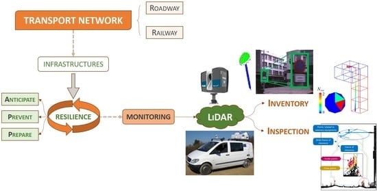
1. Introduction
- (1)
- An extensive literature review that describes different methods and applications for the monitoring of terrestrial transportation networks using data collected from Mobile Mapping Systems equipped with LiDAR sensors, with a focus on infrastructure assets whose analysis is relevant in the context of transport network resilience.
- (2)
- A descriptive summary of different laser scanner systems and their components, together with a comparison of commercial systems.
- (3)
- A special focus on railway network monitoring, which in this work is classified based on the application and extensively reviewed.
- (4)
- A remark on the most recent trends regarding methods and algorithms, with a focus on supervised learning and its most recent trend, deep learning.
- (5)
- A discussion on the main challenges and future trends for laser scanner technologies.
2. Laser Scanner Technology
2.1. Laser Scanner System Components
2.1.1. LiDAR
2.1.2. Positioning and Navigation Systems
2.2. Performance Of Laser Scanning Systems
Comparison of Monitoring Technologies
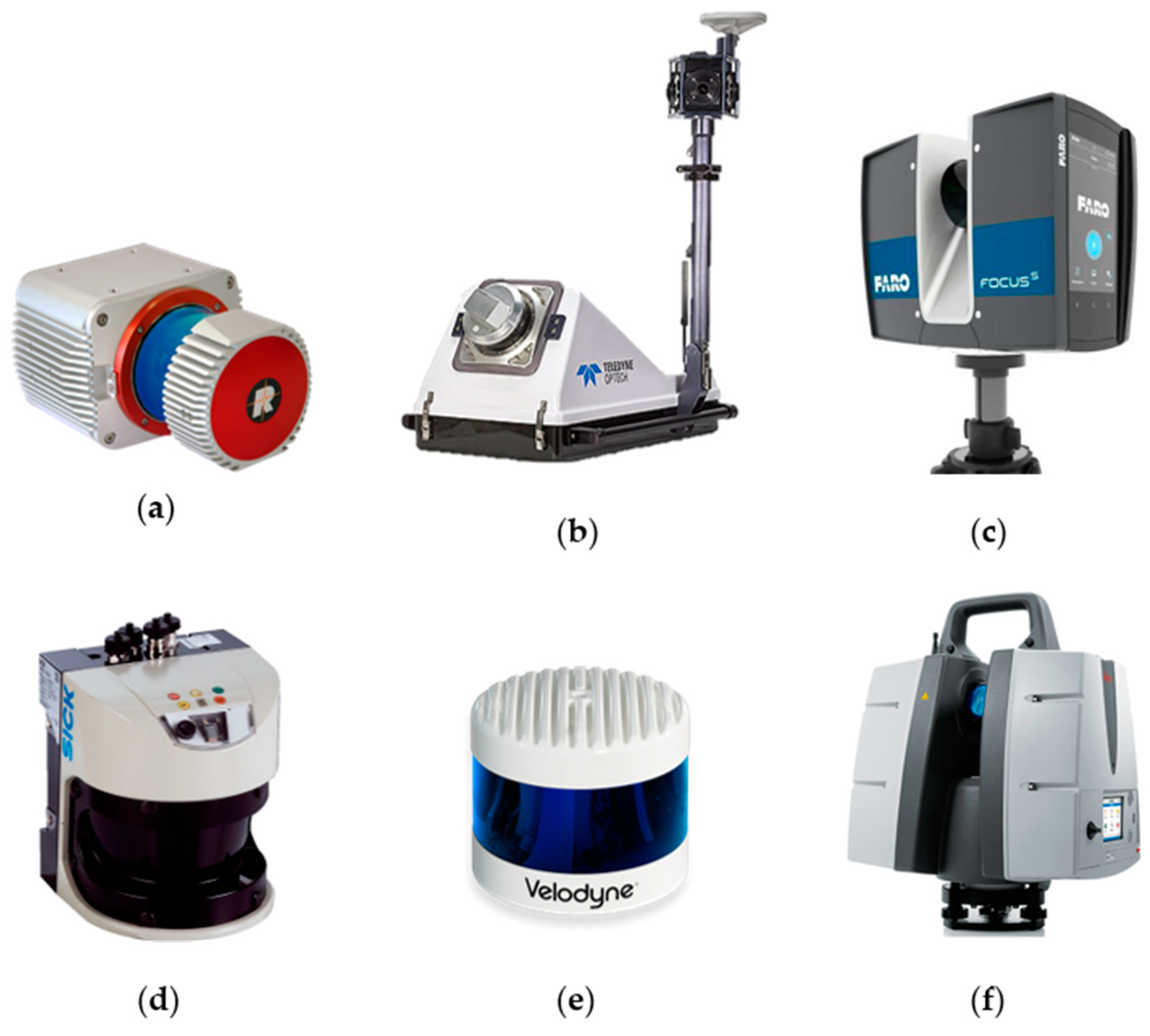
2.3. Types of Laser Scanner Systems
2.4. Comparison of Commercial Laser Scanners
3. State-of-the-Art regarding LiDAR-Based Monitoring of Transport Infrastructures
3.1. Road Network Monitoring
3.1.1. Road Surface Monitoring
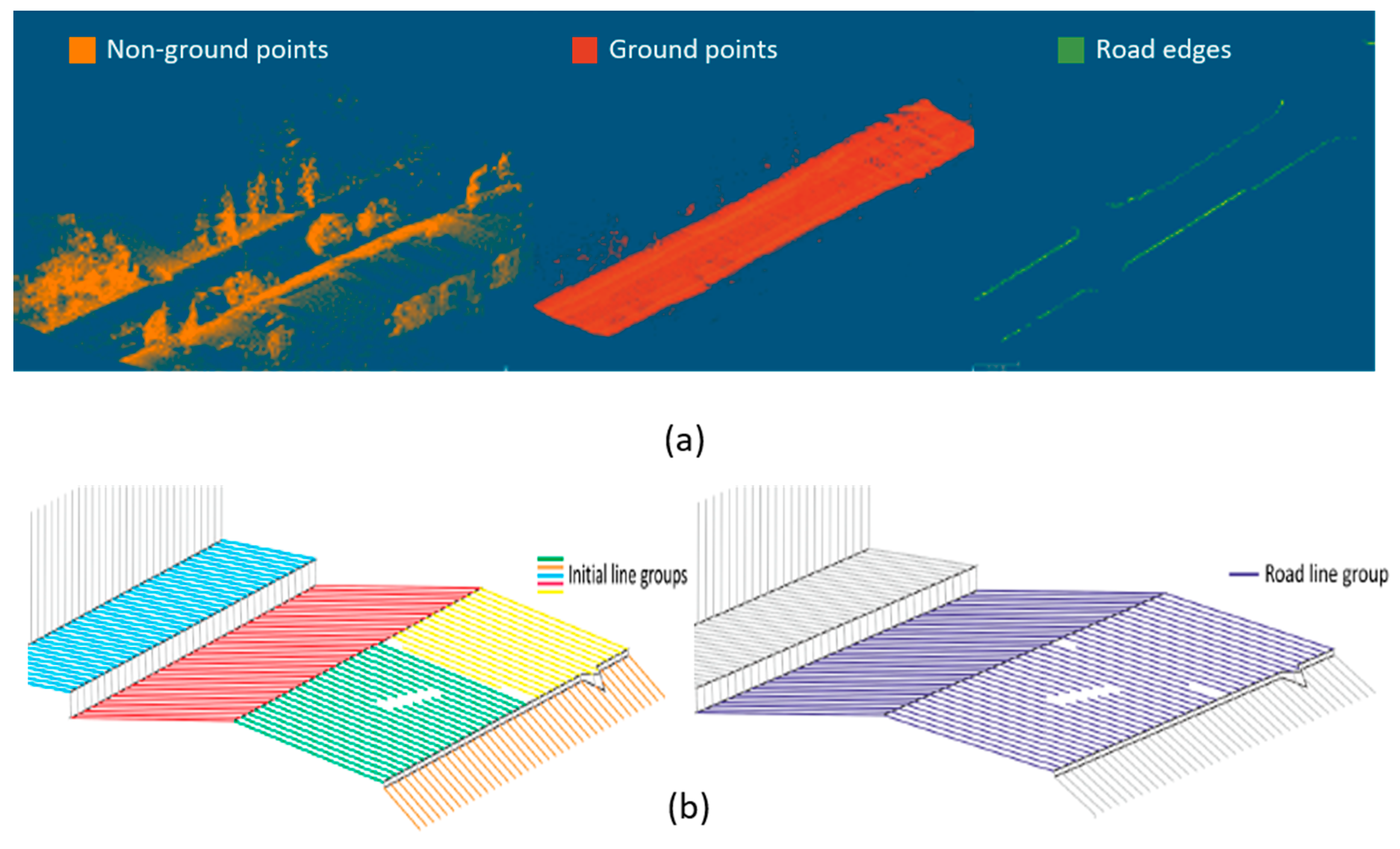
- Road surface extraction based on its structure: A common approach for road surface extraction relies on the definition of road edges that delineate its limits. This approach has been evolving since the beginning of this decade. Ibrahim and Lichti [50] propose a sequential analysis that segments the ground based on the point density and then using a Gaussian filtering to detect curbs and extract the road surface afterwards (Figure 3a). These steps are analogous in similar works, changing the curb detection method. Some works perform a rasterization (projection of the 3D point cloud in a gridded XY plane generating two dimensional geo-referenced feature (2D GRF) images) and detect curbs using image processing methods such as the parametric active contour or snake model [51,52] or image morphology [53,54]. Guan et al. [55] generate pseudo-scan lines in the plane perpendicular to the trajectory of the vehicle to detect curbs by measuring slope differences. Differently, a number of approaches have been developed for curb detection directly in 3D data using point cloud geometric properties such as density and elevation [56], or derived properties such as saliency, which measures the orientation of a point normal vector with respect to the ground plane normal vector [57] and has been successfully used to extract curbs or salient points in different works [58,59]. Xu et al. [60] use an energy function based on the elevation gradient of previously generated voxels (3D equivalent of pixels) to extract curbs, and a least cost path model to refine them. Using voxels allows one to define local information by defining parameters within each voxel and to reduce the computational load, so they are commonly used for road extraction [61,62]. Hata et al. [63] propose a robust regression method named Least Trimmed Squares (LTS) to deal with occlusions that may cause discontinuities on road edge detection. A different approach can be found in Cabo et al. [64], where the point cloud is transformed into a structured line cloud and lines are grouped to detect the edges (Figure 3b). Although good results can be found among these works, most of them rely on curbs to define road edges, hence the extraction of the road surface will not be robust when it is not delimited by curbs, as is the case in most non-urban roads.
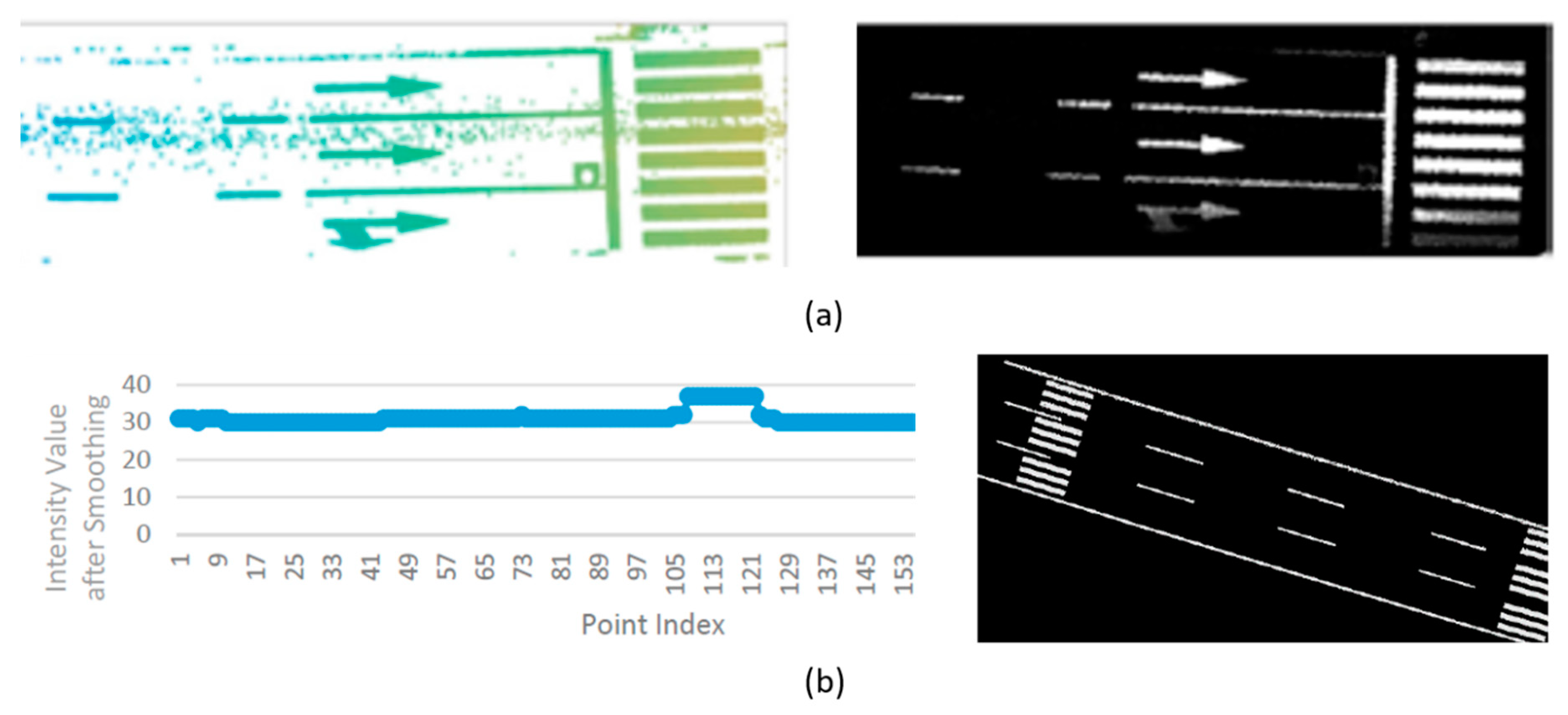
- Road surface extraction based on feature calculation: A different approach for road surface extraction is based on previous knowledge about its geometry and contextual features, which can be identified on the 3D point cloud data. Guo et al. [65] filter points based on their height with respect to the ground and then extract the road surface via TIN (Triangulated Irregular Network) filter refinement. Generally, the elevation coordinate of the point cloud is the key feature that is employed for road surface extraction: Serna and Marcotegui [66,67] defined the -flat zones algorithm, which analyses the local height difference of the point cloud projected on the XY plane. Additionally, Fan et al. [68] employ a height histogram for detecting ground points as a pre-processing step on an object detection application. Another feature that is commonly used is the roughness of the road surface. Díaz–Vilariño et al. [69] present an analysis of roughness descriptors that are able to classify different types of road pavements (stone, asphalt) with accuracy. Similarly, Yadav et al. [70] employ roughness, together with radiometric features (assuming uniform intensity as a property of the road) and 2D point density, to delineate road surfaces from non-road surfaces. As it was the case for curb detection methods, there are scan line-based methods that rely on the point topology [71] or density [72] across the scan line for extracting the road surface.
3.1.2. Off-Road Surface Monitoring
3.1.3. Current and Future Trends
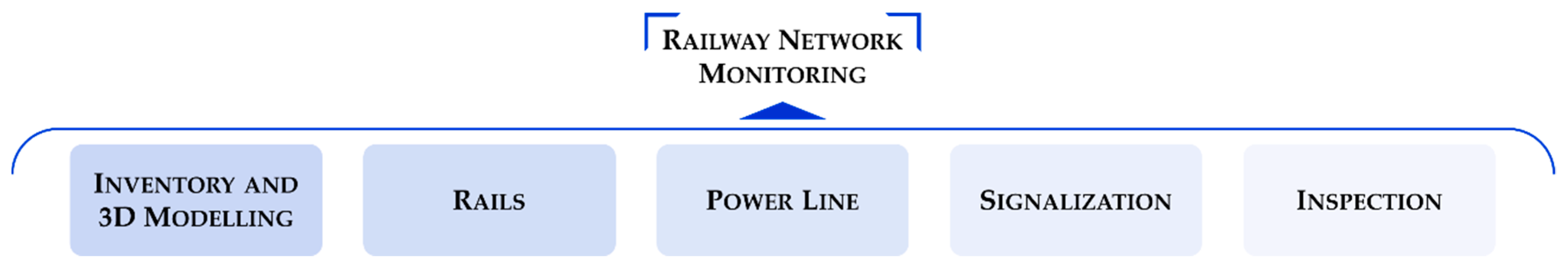
3.2. Railway Network Monitoring
3.2.1. Railway Inventory and 3D Modelling
3.2.2. Rails
3.2.3. Power Line
3.2.4. Signalization
3.2.5. Inspection
4. Conclusions
Author Contributions
Funding
Acknowledgments
Conflicts of Interest
References
- European Commission EU Transport in Figures. Statistical Pocketbook; Publications Office of the European Union: Luxembourg, 2018. [Google Scholar]
- European Commission Transport in the European Union. Current Trends and Issues; European Commission, Directorate-General Mobility and Transport: Brussels, Belgium, 2019. [Google Scholar]
- European Union Road Federation (ERF). An ERF Position Paper for Maintaining and Improving a Sustainable and Efficient Road Network; ERF: Brussels, Belgium, 2015. [Google Scholar]
- tCat-Disrupting the Rail Maintenance Sector Thanks to the Most Cost-Efficient Solution to Auscultate Railways Overhead Lines Reducing Costs up to 80%. Available online: https://cordis.europa.eu/project/rcn/211356/factsheet/en (accessed on 20 June 2019).
- AutoScan. Available online: https://cordis.europa.eu/project/rcn/203338/factsheet/en (accessed on 20 June 2019).
- NeTIRail-INFRA. Available online: https://cordis.europa.eu/project/rcn/193387/factsheet/en (accessed on 20 June 2019).
- Fortunato, G.; Funari, M.F.; Lonetti, P. Survey and seismic vulnerability assessment of the Baptistery of San Giovanni in Tumba (Italy). J. Cult. Herit. 2017, 26, 64–78. [Google Scholar] [CrossRef]
- Rowlands, K.A.; Jones, L.D.; Whitworth, M. Landslide Laser Scanning: A new look at an old problem. Q. J. Eng. Geol. Hydrogeol. 2003, 36, 155–157. [Google Scholar] [CrossRef]
- Puente, I.; González-Jorge, H.; Martínez-Sánchez, J.; Arias, P. Review of mobile mapping and surveying technologies. Meas. J. Int. Meas. Confed. 2013, 46, 2127–2145. [Google Scholar] [CrossRef]
- Williams, K.; Olsen, M.J.; Roe, G.V.; Glennie, C. Synthesis of Transportation Applications of Mobile LIDAR. Remote Sens. 2013, 5, 4652–4692. [Google Scholar] [CrossRef] [Green Version]
- Guan, H.; Li, J.; Cao, S.; Yu, Y. Use of mobile LiDAR in road information inventory: A review. Int. J. Image Data Fusion 2016, 7, 219–242. [Google Scholar] [CrossRef]
- Gargoum, S.; El-Basyouny, K. Automated extraction of road features using LiDAR data: A review of LiDAR applications in transportation. In Proceedings of the 2017 4th International Conference on Transportation Information and Safety (ICTIS), Banff, AB, Canada, 8–10 August 2017; pp. 563–574. [Google Scholar]
- Ma, L.; Li, Y.; Li, J.; Wang, C.; Wang, R.; Chapman, M.A. Mobile laser scanned point-clouds for road object detection and extraction: A review. Remote Sens. 2018, 10, 1531. [Google Scholar] [CrossRef]
- Wang, R.; Peethambaran, J.; Chen, D. LiDAR Point Clouds to 3-D Urban Models: A Review. IEEE J. Sel. Top. Appl. Earth Obs. Remote Sens. 2018, 11, 606–627. [Google Scholar] [CrossRef]
- Che, E.; Jung, J.; Olsen, M.J. Object recognition, segmentation, and classification of mobile laser scanning point clouds: A state of the art review. Sensors 2019, 19, 810. [Google Scholar] [CrossRef] [PubMed]
- SCOPUS. Available online: http://0-www-scopus-com.brum.beds.ac.uk/ (accessed on 28 June 2019).
- Tao, C.V. Mobile mapping technology for road network data acquisition. J. Geospat. Eng. 2000, 2, 1–14. [Google Scholar]
- Wehr, A.; Lohr, U. Airborne laser scanning—An introduction and overview. ISPRS J. Photogramm. Remote Sens. 1999, 54, 68–82. [Google Scholar] [CrossRef]
- Kashani, A.G.; Olsen, M.J.; Parrish, C.E.; Wilson, N. A review of LIDAR radiometric processing: From ad hoc intensity correction to rigorous radiometric calibration. Sensors 2015, 15, 28099–28128. [Google Scholar] [CrossRef] [PubMed]
- Armesto-González, J.; Riveiro-Rodríguez, B.; González-Aguilera, D.; Rivas-Brea, M.T. Terrestrial laser scanning intensity data applied to damage detection for historical buildings. J. Archaeol. Sci. 2010, 37, 3037–3047. [Google Scholar] [CrossRef]
- Wagner, W.; Ullrich, A.; Melzer, T.; Briese, C.; Kraus, K. From single-pulse to full-waveform airborne laser scanners: Potential and practical challenges. Int. Arch. Photogramm. Remote Sens. Spat. Inf. Sci. 2004, XXXV, 201–206. [Google Scholar]
- Wagner, W.; Ullrich, A.; Ducic, V.; Melzer, T.; Studnicka, N. Gaussian decomposition and calibration of a novel small-footprint full-waveform digitising airborne laser scanner. ISPRS J. Photogramm. Remote Sens. 2006, 60, 100–112. [Google Scholar] [CrossRef]
- Kais, M.; Bonnifait, P.; Bétaille, D.; Peyret, F. Development of loosely-coupled FOG/DGPS and FOG/RTK systems for ADAS and a methodology to assess their real-time performances. In Proceedings of the IEEE Intelligent Vehicles Symposium, Las Vegas, NV, USA, 6–8 June 2005; pp. 358–363. [Google Scholar]
- Welch, G.; Bishop, G.; Hill, C. An Introduction to the Kalman Filter; Technical Report; Univresity of North Carolina: Chapel Hill, NC, USA, 2002. [Google Scholar]
- Yoo, H.J.; Goulette, F.; Senpauroca, J.; Lepère, G. Analysis and Improvement of Laser Terrestrial Mobile Mapping Systems Configurations. Int. Arch. Photogramm. Remote Sens. Spat. Inf. Sci. 2010, 38, 633–638. [Google Scholar]
- Kiziltas, S.; Akinci, B.; Ergen, E.; Tang, P.; Gordon, C. Technological assessment and process implications of field data capture technologies for construction and facility/infrastructure management. Electron. J. Inf. Technol. Constr. 2008, 13, 134–154. [Google Scholar]
- Golparvar-Fard, M.; Bohn, J.; Teizer, J.; Savarese, S.; Peña-Mora, F. Evaluation of image-based modeling and laser scanning accuracy for emerging automated performance monitoring techniques. Autom. Constr. 2011, 20, 1143–1155. [Google Scholar] [CrossRef]
- Park, H.S.; Lee, H.M.; Adeli, H.; Lee, I. A new approach for health monitoring of structures: Terrestrial laser scanning. Comput. Civ. Infrastruct. Eng. 2007, 22, 19–30. [Google Scholar] [CrossRef]
- Dai, F.; Rashidi, A.; Brilakis, I.; Vela, P. Comparison of Image-Based and Time-of-Flight-Based Technologies for Three-Dimensional Reconstruction of Infrastructure. J. Constr. Eng. Manag. 2012, 139, 69–79. [Google Scholar] [CrossRef]
- Ingensand, H. Metrological Aspects in Terrestrial Laser-Scanning Technology. In Proceedings of the 3rd IAG/12th FIG Symposium, Baden, Germany, 22–24 May 2006. [Google Scholar]
- Beraldin, J.A.; Blais, F.; Boulanger, P.; Cournoyer, L.; Domey, J.; El-Hakim, S.F.; Godin, G.; Rioux, M.; Taylor, J. Real world modelling through high resolution digital 3D imaging of objects and structures. ISPRS J. Photogramm. Remote Sens. 2000, 55, 230–250. [Google Scholar] [CrossRef]
- Golparvar-Fard, M.; Peña-Mora, F.; Savarese, S. D 4 AR—A 4-Dimensional augmented reality model for automating construction progress data collection, processing and communication. J. Inf. Technol. Constr. 2009, 14, 129–153. [Google Scholar]
- Zhu, L.; Hyyppä, J.; Kukko, A.; Kaartinen, H.; Chen, R. Photorealistic building reconstruction from mobile laser scanning data. Remote Sens. 2011, 3, 1406–1426. [Google Scholar] [CrossRef]
- Olsen, M.J.; Asce, M.; Kuester, F.; Chang, B.J.; Asce, S.M.; Hutchinson, T.C.; Asce, M. Terrestrial Laser Scanned-Based Structural Damage Assessment. J. Comput. Civ. Eng. 2010, 24. [Google Scholar] [CrossRef]
- Kobler, A.; Pfeifer, N.; Ogrinc, P.; Todorovski, L.; Oštir, K.; Džeroski, S. Repetitive interpolation: A robust algorithm for DTM generation from Aerial Laser Scanner Data in forested terrain. Remote Sens. Environ. 2007, 108, 9–23. [Google Scholar] [CrossRef]
- Jaakkola, A.; Hyyppä, J.; Hyyppä, H.; Kukko, A. Retrieval algorithms for road surface modelling using laser-based mobile mapping. Sensors 2008, 8, 5238–5249. [Google Scholar] [CrossRef] [PubMed]
- Kukko, A.; Kaartinen, H.; Hyyppä, J.; Chen, Y. Multiplatform mobile laser scanning: Usability and performance. Sensors 2012, 12, 11712–11733. [Google Scholar] [CrossRef]
- Pu, S.; Rutzinger, M.; Vosselman, G.; Oude Elberink, S. Recognizing basic structures from mobile laser scanning data for road inventory studies. ISPRS J. Photogramm. Remote Sens. 2011, 66, S28–S39. [Google Scholar] [CrossRef]
- Ellum, C.; El-sheimy, N. The development of a backpack mobile mapping system. Archives 2000, 33, 184–191. [Google Scholar]
- RIEGL—Homepage of the Company RIEGL Laser Measurement Systems GmbH. Available online: http://www.riegl.com/ (accessed on 28 June 2019).
- Teledyne Optech. Available online: https://www.teledyneoptech.com/en/home/ (accessed on 28 June 2019).
- FARO—Homepage of the Company Faro Technologies, Inc. Available online: https://velodynelidar.com/ (accessed on 28 June 2019).
- VELODYNE—Homepage of the Company Velodyne Lidar, Inc. Available online: https://velodynelidar.com/ (accessed on 28 June 2019).
- SICK—Homepage of the Company Sick AG. Available online: https://www.sick.com/gb/en (accessed on 28 June 2019).
- LEICA HEXAGON-Homepage of the company Leica Geosystems AG. Available online: https://leica-geosystems.com/ (accessed on 28 June 2019).
- Link, L.E.; Collins, J.G. Airborne laser systems use in terrain mapping. In Proceedings of the 15th International Symposium on Remote Sensing of Environment, Ann Arbor, MI, USA, 11–15 May 1981; pp. 95–110. [Google Scholar]
- Riveiro, B.; González-Jorge, H.; Conde, B.; Puente, I. Laser Scanning Technology: Fundamentals, Principles and Applications in Infrastructure. In Non-Destructive Techniques for the Reverse Engineering of Structures and Infrastructure; CRC Press: London, UK, 2016; Volume 11, pp. 7–33. [Google Scholar]
- Lohr, U. Digital elevation models by laser scanning. Photogramm. Rec. 1998, 16, 105–109. [Google Scholar] [CrossRef]
- Sithole, G. Filtering of Laser Altimetry Data Using a Slope Adaptive Filter. Int. Arch. Photogramm. Remote Sens. Spat. Inf. Sci. 2001, 34, 203–210. [Google Scholar]
- Ibrahim, S.; Lichti, D. Curb-based street floor extraction from mobile terrestrial lidar point cloud. ISPRS-Int. Arch. Photogramm. Remote Sens. Spat. Inf. Sci. 2012, 39, B5. [Google Scholar] [CrossRef]
- Kumar, P.; McElhinney, C.P.; Lewis, P.; McCarthy, T. An automated algorithm for extracting road edges from terrestrial mobile LiDAR data. ISPRS J. Photogramm. Remote Sens. 2013, 85, 44–55. [Google Scholar] [CrossRef] [Green Version]
- Kumar, P.; Lewis, P.; McCarthy, T. The Potential of Active Contour Models in Extracting Road Edges from Mobile Laser Scanning Data. Infrastructures 2017, 2, 9. [Google Scholar] [CrossRef]
- Rodríguez-Cuenca, B.; García-Cortés, S.; Ordóñez, C.; Alonso, M.C. An approach to detect and delineate street curbs from MLS 3D point cloud data. Autom. Constr. 2015, 51, 103–112. [Google Scholar] [CrossRef]
- Rodríguez-Cuenca, B.; García-Cortés, S.; Ordóñez, C.; Alonso, M. Morphological Operations to Extract Urban Curbs in 3D MLS Point Clouds. ISPRS Int. J. Geo-Inf. 2016, 5, 93. [Google Scholar] [CrossRef]
- Guan, H.; Li, J.; Yu, Y.; Wang, C.; Chapman, M.; Yang, B. Using mobile laser scanning data for automated extraction of road markings. ISPRS J. Photogramm. Remote Sens. 2014, 87, 93–107. [Google Scholar] [CrossRef]
- Yang, B.; Fang, L.; Li, J. Semi-automated extraction and delineation of 3D roads of street scene from mobile laser scanning point clouds. ISPRS J. Photogramm. Remote Sens. 2013, 79, 80–93. [Google Scholar] [CrossRef]
- Wang, H.; Luo, H.; Wen, C.; Cheng, J.; Li, P.; Chen, Y.; Wang, C.; Li, J. Road Boundaries Detection Based on Local Normal Saliency From Mobile Laser Scanning Data. IEEE Geosci. Remote Sens. Lett. 2015, 12, 2085–2089. [Google Scholar] [CrossRef]
- Soilán, M.; Riveiro, B.; Sánchez-Rodríguez, A.; Arias, P. Safety assessment on pedestrian crossing environments using MLS data. Accid. Anal. Prev. 2018, 111, 328–337. [Google Scholar] [CrossRef]
- Sánchez-Rodríguez, A.; Riveiro, B.; Soilán, M.; González-deSantos, L.M. Automated detection and decomposition of railway tunnels from Mobile Laser Scanning Datasets. Autom. Constr. 2018, 96, 171–179. [Google Scholar] [CrossRef]
- Xu, S.; Wang, R.; Zheng, H. Road curb extraction from mobile LiDAR point clouds. IEEE Trans. Geosci. Remote Sens. 2017, 55, 996–1009. [Google Scholar] [CrossRef]
- Douillard, B.; Underwood, J.; Kuntz, N.; Vlaskine, V.; Quadros, A.; Morton, P.; Frenkel, A. On the segmentation of 3D lidar point clouds. In Proceedings of the IEEE International Conference on Robotics and Automation, Shanghai, China, 9–13 May 2011; pp. 2798–2805. [Google Scholar]
- Zai, D.; Li, J.; Guo, Y.; Cheng, M.; Lin, Y.; Luo, H.; Wang, C. 3-D Road Boundary Extraction from Mobile Laser Scanning Data via Supervoxels and Graph Cuts. IEEE Trans. Intell. Transp. Syst. 2018, 19, 802–813. [Google Scholar] [CrossRef]
- Hata, A.Y.; Osorio, F.S.; Wolf, D.F. Robust curb detection and vehicle localization in urban environments. In Proceedings of the IEEE Intelligent Vehicles Symposium Proceedings, Dearborn, MI, USA, 8–11 June 2014; pp. 1257–1262. [Google Scholar]
- Cabo, C.; Kukko, A.; García-Cortés, S.; Kaartinen, H.; Hyyppä, J.; Ordoñez, C. An algorithm for automatic road asphalt edge delineation from mobile laser scanner data using the line clouds concept. Remote Sens. 2016, 8, 740. [Google Scholar] [CrossRef]
- Guo, J.; Tsai, M.-J.; Han, J.-Y. Automatic reconstruction of road surface features by using terrestrial mobile lidar. Autom. Constr. 2015, 58, 165–175. [Google Scholar] [CrossRef]
- Serna, A.; Marcotegui, B. Urban accessibility diagnosis from mobile laser scanning data. ISPRS J. Photogramm. Remote Sens. 2013, 84, 23–32. [Google Scholar] [CrossRef] [Green Version]
- Serna, A.; Marcotegui, B. Detection, segmentation and classification of 3D urban objects using mathematical morphology and supervised learning. ISPRS J. Photogramm. Remote Sens. 2014, 93, 243–255. [Google Scholar] [CrossRef] [Green Version]
- Fan, H.; Yao, W.; Tang, L. Identifying man-made objects along urban road corridors from mobile lidar data. IEEE Geosci. Remote Sens. Lett. 2013, 11, 950–954. [Google Scholar] [CrossRef]
- Díaz-Vilariño, L.; González-Jorge, H.; Bueno, M.; Arias, P.; Puente, I. Automatic classification of urban pavements using mobile LiDAR data and roughness descriptors. Constr. Build. Mater. 2016, 102, 208–215. [Google Scholar] [CrossRef]
- Yadav, M.; Singh, A.K.; Lohani, B. Extraction of road surface from mobile LiDAR data of complex road environment. Int. J. Remote Sens. 2017, 38, 4645–4672. [Google Scholar] [CrossRef]
- Ying Zhou; Dan Wang; Xiang Xie; Yiyi Ren; Guolin Li; Yangdong Deng; Zhihua Wang A Fast and Accurate Segmentation Method for Ordered LiDAR Point Cloud of Large-Scale Scenes. IEEE Geosci. Remote Sens. Lett. 2014, 11, 1981–1985. [CrossRef]
- Che, E.; Olsen, M.J. Fast ground filtering for TLS data via Scanline Density Analysis. ISPRS J. Photogramm. Remote Sens. 2017, 129, 226–240. [Google Scholar] [CrossRef]
- Soilán, M.; Riveiro, B.; Martínez-Sánchez, J.; Arias, P. Segmentation and classification of road markings using MLS data. ISPRS J. Photogramm. Remote Sens. 2017, 123, 94–103. [Google Scholar] [CrossRef]
- Riveiro, B.; González-Jorge, H.; Martínez-Sánchez, J.; Díaz-Vilariño, L.; Arias, P. Automatic detection of zebra crossings from mobile LiDAR data. Opt. Laser Technol. 2015, 70, 63–70. [Google Scholar] [CrossRef]
- Arias, P.; Riveiro, B.; Soilán, M.; Díaz-Vilariño, L.; Martínez-Sánchez, J. Simple Approaches To Improve the Automatic Inventory of Zebra Crossing From Mls Data. ISPRS Int. Arch. Photogramm. Remote Sens. Spat. Inf. Sci. 2015, 40, 103–108. [Google Scholar] [CrossRef]
- Guan, H.; Li, J.; Member, S.; Yu, Y.; Ji, Z.; Wang, C. Using Mobile LiDAR Data for Rapidly Updating Road Markings. IEEE Trans. Intell. Transp. Syst. 2015, 16, 2457–2466. [Google Scholar] [CrossRef]
- Ma, L.; Li, Y.; Li, J.; Zhong, Z.; Chapman, M.A. Generation of Horizontally Curved Driving Lines in HD Maps Using Mobile Laser Scanning Point Clouds. IEEE J. Sel. Top. Appl. Earth Obs. Remote Sens. 2019, 12, 1572–1586. [Google Scholar] [CrossRef]
- Yan, L.; Liu, H.; Tan, J.; Li, Z.; Xie, H.; Chen, C. Scan line based road marking extraction from mobile LiDAR point clouds. Sensors 2016, 16, 903. [Google Scholar] [CrossRef] [PubMed]
- Yu, Y.; Li, J.; Guan, H.; Jia, F.; Wang, C. Learning Hierarchical Features for Automated Extraction of Road Markings From 3-D Mobile LiDAR Point Clouds. IEEE J. Sel. Top. Appl. Earth Obs. Remote Sens. 2015, 8, 709–726. [Google Scholar] [CrossRef]
- Jung, J.; Che, E.; Olsen, M.J.; Parrish, C. Efficient and robust lane marking extraction from mobile lidar point clouds. ISPRS J. Photogramm. Remote Sens. 2019, 147, 1–18. [Google Scholar] [CrossRef]
- Wen, C.; Sun, X.; Li, J.; Wang, C.; Guo, Y.; Habib, A. A deep learning framework for road marking extraction, classification and completion from mobile laser scanning point clouds. ISPRS J. Photogramm. Remote Sens. 2019, 147, 178–192. [Google Scholar] [CrossRef]
- Zhao, H. Recognizing Features in Mobile Laser Scanning Point Clouds Towards 3D High-Definition Road Maps for Autonomous Vehicles. Master’s Thesis, University of Waterloo, Waterloo, Belgium, 2017. [Google Scholar]
- Ye, C.; Li, J.; Member, S.; Jiang, H. Semi-Automated Generation of Road Transition Lines Using Mobile Laser Scanning Data. IEEE Trans. Intell. Transp. Syst. 2019, 1–14. [Google Scholar] [CrossRef]
- Ding, L.; Zhang, H.; Li, B.; Xiao, J.; Lu, S.; Klette, R. Improved road marking detection and recognition. In Proceedings of the 15th International Symposium on Pervasive Systems, Algorithms and Networks (I-SPAN), Yichang, China, 16–18 October 2018. [Google Scholar]
- Li, J.; Mei, X.; Prokhorov, D.; Tao, D. Deep Neural Network for Structural Prediction and Lane Detection in Traffic Scene. IEEE Trans. Neural Netw. Learn. Syst. 2016, 28, 690–713. [Google Scholar] [CrossRef] [PubMed]
- Jia, H.; Wei, Z.; He, X.; Lv, Y.; He, D.; Li, M. Biologically Visual Perceptual Model and Discriminative Model for Road Markings Detection and Recognition. Math. Probl. Eng. 2018, 2018, 6062081. [Google Scholar] [CrossRef]
- Tian, Y.; Gelernter, J.; Wang, X.; Chen, W.; Gao, J.; Zhang, Y.; Li, X. Lane marking detection via deep convolutional neural network. Neurocomputing 2018, 280, 46–55. [Google Scholar] [CrossRef] [PubMed]
- Kim, H.; Liu, B.; Myung, H. Road-feature extraction using point cloud and 3D LiDAR sensor for vehicle localization. In Proceedings of the 14th International Conference on Ubiquitous Robots and Ambient Intelligence (URAI), Jeju, Korea, 28 June–1 July 2017; Volume 2, pp. 891–892. [Google Scholar]
- Yu, Y.; Li, J.; Guan, H.; Wang, C. 3D crack skeleton extraction from mobile LiDAR point clouds. In Proceedings of the Geoscience and Remote Sensing Symposium, Quebec, QC, Canada, 13–18 July 2014; pp. 914–917. [Google Scholar] [CrossRef]
- Guan, H.; Li, J.; Yu, Y.; Chapman, M.; Wang, H.; Wang, C.; Zhai, R. Iterative tensor voting for pavement crack extraction using mobile laser scanning data. IEEE Trans. Geosci. Remote Sens. 2015, 53, 1527–1537. [Google Scholar] [CrossRef]
- Chen, X.; Li, J.; Cloud, P.; Crack, P.; Detection, A.; Road, U.; Canada, I. A feasibility study on use of generic mobile laser scanning system. Proc. Int. Arch. Photogramm. Remote Sens. Spat. Inf. Sci. 2016, XLI, 545–549. [Google Scholar] [CrossRef]
- Gavilán, M.; Balcones, D.; Marcos, O.; Llorca, D.F.; Sotelo, M.A. Adaptive Road Crack Detection System by Pavement Classification. Sensors 2011, 11, 9628–9657. [Google Scholar] [CrossRef]
- Venmans, A.A.M.; Van De Ven, R.; Kollen, J. Rapid and Non-intrusive Measurements of Moisture in Road Constructions Using Passive Microwave Radiometry and GPR-Full Scale Test. Procedia Eng. 2016, 143, 1244–1251. [Google Scholar] [CrossRef]
- Aparna; Bhatia, Y.; Rai, R.; Gupta, V.; Aggarwal, N.; Akula, A. Convolutional neural networks based potholes detection using thermal imaging. J. King Saud Univ.-Comput. Inf. Sci. 2019, in press. [Google Scholar] [CrossRef]
- Guan, H.; Yu, Y.; Li, J.; Liu, P.; Zhao, H.; Wang, C. Automated extraction of manhole covers using mobile LiDAR data. Remote Sens. Lett. 2014, 5, 1042–1050. [Google Scholar] [CrossRef]
- Yu, Y.; Guan, H.; Ji, Z. Automated Detection of Urban Road Manhole Covers Using Mobile Laser Scanning Data. IEEE Trans. Intell. Transp. Syst. 2015, 16, 3258–3269. [Google Scholar] [CrossRef]
- Ai, C.; Tsai, Y.J. An automated sign retroreflectivity condition evaluation methodology using mobile LIDAR and computer vision. Transp. Res. Part C Emerg. Technol. 2016, 63, 96–113. [Google Scholar] [CrossRef]
- Ai, C.; Tsai, Y.-C.J. Critical Assessment of an Enhanced Traffic Sign Detection Method Using Mobile LiDAR and INS Technologies. J. Transp. Eng. 2014, 141, 04014096. [Google Scholar] [CrossRef]
- Riveiro, B.; Diaz-Vilariño, L.; Conde, B.; Soilán, M.; Arias, P. Automatic Segmentation and Shape-Based Classification of Retro-Reflective Traffic Signs from Mobile LiDAR Data. IEEE J. Sel. Top. Appl. Earth Obs. Remote Sens. 2016, 9, 295–303. [Google Scholar] [CrossRef]
- Soilán, M.; Riveiro, B.; Martínez-Sánchez, J.; Arias, P. Traffic sign detection in MLS acquired point clouds for geometric and image-based semantic inventory. ISPRS J. Photogramm. Remote Sens. 2016, 114, 92–101. [Google Scholar] [CrossRef]
- Soilán, M.; Riveiro, B.; Martínez-Sánchez, J.; Arias, P. Automatic road sign inventory using mobile mapping systems. Int. Arch. Photogramm. Remote Sens. Spat. Inf. Sci. 2016, 41, 717–723. [Google Scholar] [CrossRef]
- Huang, P.; Cheng, M.; Chen, Y.; Luo, H.; Wang, C.; Member, S.; Li, J.; Member, S. Traffic Sign Occlusion Detection Using Mobile Laser Scanning Point Clouds. IEEE Trans. Intell. Transp. Syst. 2017, 18, 2364–2376. [Google Scholar] [CrossRef]
- Wen, C.; Li, J.; Member, S.; Luo, H.; Yu, Y.; Cai, Z.; Wang, H.; Wang, C. Spatial-Related Traffic Sign Inspection for Inventory Purposes Using Mobile Laser Scanning Data. IEEE Trans. Intell. Transp. Syst. 2015, 17, 27–37. [Google Scholar] [CrossRef]
- Guan, H.; Yan, W.; Yu, Y.; Zhong, L.; Li, D. Robust Traffic-Sign Detection and Classification Using Mobile LiDAR Data with Digital Images. IEEE J. Sel. Top. Appl. Earth Obs. Remote Sens. 2018, 11, 1715–1724. [Google Scholar] [CrossRef]
- Yu, Y.; Li, J.; Wen, C.; Guan, H.; Luo, H.; Wang, C. Bag-of-visual-phrases and hierarchical deep models for traffic sign detection and recognition in mobile laser scanning data. ISPRS J. Photogramm. Remote Sens. 2016, 113, 106–123. [Google Scholar] [CrossRef]
- Tan, M.; Wang, B.; Wu, Z.; Member, S.; Wang, J.; Pan, G. Weakly Supervised Metric Learning for Traffic Sign Recognition in a LIDAR-Equipped Vehicle. IEEE Trans. Intell. Transp. Syst. 2016, 17, 1415–1427. [Google Scholar] [CrossRef]
- Arcos-García, A.; Soilán, M.; Alvarez-García, J.A.; Belén, R. Exploiting synergies of mobile mapping sensors and deep learning for traffic sign recognition systems. Expert Syst. Appl. 2017, 89, 286–295. [Google Scholar] [CrossRef]
- Jain, A.; Mishra, A.; Shukla, A.; Tiwari, R. A Novel Genetically Optimized Convolutional Neural Network for Traffic Sign Recognition: A New Benchmark on Belgium and Chinese Traffic Sign Datasets. Neural Process. Lett. 2019. [Google Scholar] [CrossRef]
- Gudigar, A.; Chokkadi, S.; Raghavendra, U.; Acharya, U.R. An efficient traffic sign recognition based on graph embedding features. Neural Comput. Appl. 2019, 31, 395–407. [Google Scholar] [CrossRef]
- Cheng, L.; Tong, L.; Wang, Y.; Li, M. Extraction of Urban Power Lines from Vehicle-Borne LiDAR Data. Remote Sens. 2014, 6, 3302–3320. [Google Scholar] [CrossRef] [Green Version]
- Yu, Y.; Li, J.; Guan, H.; Wang, C.; Yu, J. Semiautomated Extraction of Street Light Poles From Mobile LiDAR Point-Clouds. IEEE Trans. Geosci. Remote Sens. 2015, 53, 1374–1386. [Google Scholar] [CrossRef]
- Guan, H.; Yu, Y.; Li, J.; Liu, P. Pole-Like Road Object Detection in Mobile LiDAR Data via Supervoxel and Bag-of-Contextual-Visual-Words Representation. IEEE Geosci. Remote Sens. Lett. 2016, 13, 520–524. [Google Scholar] [CrossRef]
- Yu, Y.; Li, J.; Guan, H.; Wang, C.; Wen, C. Bag of contextual-visual words for road scene object detection from mobile laser scanning data. IEEE Trans. Intell. Transp. Syst. 2016, 17, 3391–3406. [Google Scholar] [CrossRef]
- Wang, J.; Lindenbergh, R.; Menenti, M. SigVox—A 3D feature matching algorithm for automatic street object recognition in mobile laser scanning point clouds. ISPRS J. Photogramm. Remote Sens. 2017, 128, 111–129. [Google Scholar] [CrossRef]
- Rodríguez-Cuenca, B.; García-Cortés, S.; Ordóñez, C.; Alonso, M.C. Automatic detection and classification of pole-like objects in urban point cloud data using an anomaly detection algorithm. Remote Sens. 2015, 7, 12680–12703. [Google Scholar] [CrossRef]
- Yan, L.; Li, Z.; Liu, H.; Tan, J.; Zhao, S.; Chen, C. Detection and classification of pole-like road objects from mobile LiDAR data in motorway environment. Opt. Laser Technol. 2017, 97, 272–283. [Google Scholar] [CrossRef]
- Wu, F.; Wen, C.; Guo, Y.; Wang, J.; Yu, Y.; Wang, C.; Li, J. Rapid localization and extraction of street light poles in mobile LiDAR point clouds: A supervoxel-based approach. IEEE Trans. Intell. Transp. Syst. 2016, 18, 292–305. [Google Scholar] [CrossRef]
- Cabo, C.; Ordoñez, C.; García-Cortés, S.; Martínez, J. An algorithm for automatic detection of pole-like street furniture objects from Mobile Laser Scanner point clouds. ISPRS J. Photogramm. Remote Sens. 2014, 87, 47–56. [Google Scholar] [CrossRef]
- Li, L.; Li, Y.; Li, D. A method based on an adaptive radius cylinder model for detecting pole-like objects in mobile laser scanning data. Remote Sens. Lett. 2016, 7, 249–258. [Google Scholar] [CrossRef]
- Wang, H.; Wang, C.; Luo, H.; Li, P.; Chen, Y.; Li, J. 3-D Point Cloud Object Detection Based on Supervoxel Neighborhood With Hough Forest Framework. IEEE J. Sel. Top. Appl. Earth Obs. Remote Sens. 2015, 8, 1570–1581. [Google Scholar] [CrossRef]
- Teo, T.A.; Chiu, C.M. Pole-Like Road Object Detection from Mobile Lidar System Using a Coarse-to-Fine Approach. IEEE J. Sel. Top. Appl. Earth Obs. Remote Sens. 2015, 8, 4805–4818. [Google Scholar] [CrossRef]
- Xu, S.; Xu, S.; Ye, N.; Zhu, F. Automatic extraction of street trees’ nonphotosynthetic components from MLS data. Int. J. Appl. Earth Obs. Geoinf. 2018, 69, 64–77. [Google Scholar] [CrossRef]
- Guan, H.; Yu, Y.; Ji, Z.; Li, J.; Zhang, Q. Deep learning-based tree classification using mobile LiDAR data. Remote Sens. Lett. 2015, 6, 864–873. [Google Scholar] [CrossRef]
- Huang, P.; Chen, Y.; Li, J.; Yu, Y.; Wang, C.; Nie, H. Extraction of street trees from mobile laser scanning point clouds based on subdivided dimensional features. In Proceedings of the International Geoscience and Remote Sensing Symposium (IGARSS), Milan, Italy, 26–31 July 2015. [Google Scholar]
- Li, L.; Li, D.; Zhu, H.; Li, Y. A dual growing method for the automatic extraction of individual trees from mobile laser scanning data. ISPRS J. Photogramm. Remote Sens. 2016, 120, 37–52. [Google Scholar] [CrossRef]
- Zou, X.; Cheng, M.; Wang, C.; Xia, Y.; Li, J. Tree Classification in Complex Forest Point Clouds Based on Deep Learning. IEEE Geosci. Remote Sens. Lett. 2017, 14, 2360–2364. [Google Scholar] [CrossRef]
- Weinmann, M.; Weinmann, M.; Mallet, C.; Brédif, M. A classification-segmentation framework for the detection of individual trees in dense MMS point cloud data acquired in urban areas. Remote Sens. 2017, 9, 277. [Google Scholar] [CrossRef]
- Qi, C.R.; Su, H.; Mo, K.; Guibas, L.J. PointNet: Deep Learning on Point Sets for 3D Classification and Segmentation. In Proceedings of the IEEE Conference on Computer Vision and Pattern Recognition (CVPR), Honolulu, HI, USA, 21–26 July 2016; pp. 601–610. [Google Scholar] [CrossRef]
- Qi, C.R.; Yi, L.; Su, H.; Guibas, L.J. PointNet++: Deep Hierarchical Feature Learning on Point Sets in a Metric Space. In Proceedings of the 31st Conference on Neural Information Processing Systems, Long Beach, CA, USA, 4–9 December 2017. [Google Scholar]
- Tatarchenko, M.; Dosovitskiy, A.; Brox, T. Octree Generating Networks: Efficient Convolutional Architectures for High-resolution 3D Outputs. In Proceedings of the 2017 IEEE International Conference on Computer Vision (ICCV), Venice, Italy, 22–29 October 2017. [Google Scholar]
- Su, H.; Jampani, V.; Sun, D.; Maji, S.; Kalogerakis, E.; Yang, M.H.; Kautz, J. SPLATNet: Sparse Lattice Networks for Point Cloud Processing. In Proceedings of the IEEE Computer Society Conference on Computer Vision and Pattern Recognition, Salt Lake City, UT, USA, 18–23 June 2018. [Google Scholar]
- Luo, Z.; Li, J.; Xiao, Z.; Mou, Z.G.; Cai, X.; Wang, C. Learning high-level features by fusing multi-view representation of MLS point clouds for 3D object recognition in road environments. ISPRS J. Photogramm. Remote Sens. 2019, 150, 44–58. [Google Scholar] [CrossRef]
- Kumar, B.; Pandey, G.; Lohani, B.; Misra, S.C. A multi-faceted CNN architecture for automatic classification of mobile LiDAR data and an algorithm to reproduce point cloud samples for enhanced training. ISPRS J. Photogramm. Remote Sens. 2019, 147, 80–89. [Google Scholar] [CrossRef]
- Arastounia, M. An Enhanced Algorithm for Concurrent Recognition of Rail Tracks and Power Cables from Terrestrial and Airborne LiDAR Point Clouds. Infrastructures 2017, 2, 8. [Google Scholar] [CrossRef]
- Soni, A.; Robson, S.; Gleeson, B. Extracting Rail Track Geometry from Static Terrestrial Laser Scans for Monitoring Purposes. ISPRS-Int. Arch. Photogramm. Remote Sens. Spat. Inf. Sci. 2014, XL-5, 553–557. [Google Scholar] [CrossRef] [Green Version]
- Collin, B.; Carreaud, P.; Lançon, H. High Efficiency Techniques for the Assessment of Railways Infrastructures and Buildings. Transp. Res. Procedia 2016, 14, 1865–1874. [Google Scholar] [CrossRef] [Green Version]
- Lou, Y.; Zhang, T.; Tang, J.; Song, W.; Zhang, Y.; Chen, L. A Fast Algorithm for Rail Extraction Using Mobile Laser Scanning Data. Remote Sens. 2018, 10, 1998. [Google Scholar] [CrossRef]
- Arastounia, M. Automatic Classification of LiDAR Point Clouds in A Railway Environment. Master’s Thesis, University of Twente, Faculty of Geo-Information and Earth Observation, Enschede, The Netherlands, 2012. [Google Scholar]
- Beger, R.; Gedrange, C.; Hecht, R.; Neubert, M. Data fusion of extremely high resolution aerial imagery and LiDAR data for automated railroad centre line reconstruction. ISPRS J. Photogramm. Remote Sens. 2011, 66, S40–S51. [Google Scholar] [CrossRef]
- Neubert, M.; Hecht, R.; Gedrange, C.; Trommler, M.; Herold, H.; Kruger, T.; Brimmer, F. Extraction of Railroad Objects From Very High Resolution Helicopter-Borne Lidar and Ortho-Image Data. ISPRS Int. Arch. Photogramm. Remote Sens. Spat. Inf. Sci 2008, 38, 25–30. [Google Scholar]
- Zhu, L.; Hyyppa, J. The Use of Airborne and Mobile Laser Scanning for Modeling Railway Environments in 3D. Remote Sens. 2014, 6, 3075–3100. [Google Scholar] [CrossRef] [Green Version]
- Al-Bayari, O. Mobile mapping systems in civil engineering projects (case studies). Appl. Geomat. 2019, 11, 1–13. [Google Scholar] [CrossRef]
- Leslar, M.; Perry, G.; McNease, K. Using mobile lidar to survey a railway line for asset inventory. In Proceedings of the American Society for Photogrammetry and Remote Sensing Annual Conference, San Diego, CA, USA, 13 July 2010; pp. 526–533. [Google Scholar]
- Arastounia, M. Automated Recognition of Railroad Infrastructure in Rural Areas from LIDAR Data. Remote Sens. 2015, 7, 14916–14938. [Google Scholar] [CrossRef] [Green Version]
- Arastounia, M.; Elberink, S.O. Application of Template Matching for Improving Classification of Urban Railroad Point Clouds. Sensors 2016, 16, 2112. [Google Scholar] [CrossRef] [PubMed]
- Géron, A. Hands-On Machine Learning with Scikit-Learn; O’Reilly Media, Inc.: Newton, MA, USA, 2017; ISBN 9781491962299. [Google Scholar]
- Luo, C.; Jwa, Y.; Sohn, G. Context based multiple railway object recognition from mobile laser scanning data. In Proceedings of the IEEE Geoscience and Remote Sensing Symposium, Quebec, QC, Canada, 13–18 July 2014; pp. 3602–3605. [Google Scholar] [CrossRef]
- Rizaldy, A.; Persello, C.; Gevaert, C.; Elberink, S.O.; Vosselman, G. Ground and multi-class classification of Airborne Laser Scanner point clouds using Fully Convolutional Networks. Remote Sens. 2018, 10, 1723. [Google Scholar] [CrossRef]
- Kwoczynska, B.; Sagan, W.; Dziura, K. Elaboration and Modeling of the Railway Infrastructure Using Data from Airborne and Mobile Laser Scanning. In Proceedings of the Baltic Geodetic Congress (BGC Geomatics), Gdansk, Poland, 2–4 June 2016; pp. 106–115. [Google Scholar]
- Fischler, M.A.; Bolles, R.C. Random sample consensus: A paradigm for model fitting with applications to image analysis and automated cartography. Commun. ACM 1981, 24, 381–395. [Google Scholar] [CrossRef]
- Elberink, S.; Khoshelham, K. Automatic Extraction of Railroad Centerlines from Mobile Laser Scanning Data. Remote Sens. 2015, 7, 5565–5583. [Google Scholar] [CrossRef] [Green Version]
- Stein, D. Mobile Laser Scanning Based Determination of Railway Network Topology and Branching Direction on Turnouts; KIT Scientific Publishing: Karlsruhe, Germany, 2018. [Google Scholar]
- Stein, D.; Spindler, M.; Lauer, M. Model-based rail detection in mobile laser scanning data. In Proceedings of the IEEE Intelligent Vehicles Symposium, Gothenburg, Sweden, 19–22 June 2016; pp. 654–661. [Google Scholar] [CrossRef]
- Yang, B.; Fang, L. Automated extraction of 3-D railway tracks from mobile laser scanning point clouds. IEEE J. Sel. Top. Appl. Earth Obs. Remote Sens. 2014, 7, 4750–4761. [Google Scholar] [CrossRef]
- Hackel, T.; Stein, D.; Maindorfer, I.; Lauer, M.; Reiterer, A. Track detection in 3D laser scanning data of railway infrastructure. In Proceedings of the 2015 IEEE International Instrumentation and Measurement Technology Conference (I2MTC), Pisa, Italy, 11–14 May 2015; pp. 693–698. [Google Scholar]
- Jeon, W.G.; Choi, B.G. A Study on the Automatic Detection of Railroad Power Lines Using LiDAR Data and RANSAC Algorithm. J. Korean Soc. Surv. Geod. Photogramm. Cartogr. 2013, 31, 331–339. [Google Scholar] [CrossRef] [Green Version]
- Pastucha, E. Catenary System Detection, Localization and Classification Using Mobile Scanning Data. Remote Sens. 2016, 8, 801. [Google Scholar] [CrossRef]
- Zhang, S.; Wang, C.; Yang, Z.; Chen, Y.; Li, J. Automatic railway power line extraction using mobile laser scanning data. Int. Arch. Photogramm. Remote Sens. Spat. Inf. Sci. 2016, 41, 615–619. [Google Scholar] [CrossRef]
- Guo, B.; Li, Q.; Huang, X.; Wang, C. An Improved Method for Power-Line Reconstruction from Point Cloud Data. Remote Sens. 2016, 8, 36. [Google Scholar] [CrossRef]
- Fu, L.; Chang, S.; Liu, C. Automatic measuring method of catenary geometric parameters based on laser scanning and imaging. In Proceedings of the 2017 International Conference on Optical Instruments and Technology: Optoelectronic Measurement Technology and Systems, Beijing, China, 28–30 October 2017. [Google Scholar]
- Jung, J.; Chen, L.; Sohn, G.; Luo, C.; Won, J.-U. Multi-Range Conditional Random Field for Classifying Railway Electrification System Objects Using Mobile Laser Scanning Data. Remote Sens. 2016, 8, 1008. [Google Scholar] [CrossRef]
- Wang, Y.; Chen, Q.; Liu, L.; Li, K. A Hierarchical unsupervised method for power line classification from airborne LiDAR data. Int. J. Digit. Earth 2018, 1–17. [Google Scholar] [CrossRef]
- Karagiannis, G.; Olsen, S.; Pedersen, K. Deep Learning for Detection of Railway Signs and Signals. In Science and Information Conference; Springer: Berlin/Heidelberg, Germany, 2019; pp. 1–15. [Google Scholar]
- Marmo, R.; Lombardi, L.; Gagliardi, N. Railway Sign Detection and Classification. In Proceedings of the IEEE Intelligent transportation Systems Conference, Toronto, ON, Canada, 17–20 September 2006. [Google Scholar]
- Agudo, D.; Sánchez, Á.; Vélez, J.F.; Belén Moreno, A. Real-time railway speed limit sign recognition from video sequences. In Proceedings of the International Conference on Systems, Signals, and Image Processing, Bratislava, Slovakia, 23–25 May 2016. [Google Scholar]
- Falamarzi, A.; Moridpour, S.; Nazem, M. A Review on Existing Sensors and Devices for Inspecting Railway Infrastructure. J. Kejuruter. 2019, 31, 1–10. [Google Scholar]
- Minbashi, N.; Bagheri, M.; Golroo, A.; Arasteh Khouy, I.; Ahmadi, A. Turnout Degradation Modelling Using New Inspection Technologies: A Literature Review. Lect. Notes Mech. Eng. 2016, 49–63. [Google Scholar] [CrossRef]
- Blug, A.; Baulig, C.; Wolfelschneider, H.; Hofler, H. Fast fiber coupled clearance profile scanner using real time 3D data processing with automatic rail detection. In Proceedings of the IEEE Intelligent Vehicles Symposium, Parma, Italy, 14–17 June 2004; pp. 658–663. [Google Scholar]
- Mikrut, S.; Kohut, P.; Pyka, K.; Tokarczyk, R.; Barszcz, T.; Uhl, T. Mobile Laser Scanning Systems for Measuring the Clearance Gauge of Railways: State of Play, Testing and Outlook. Sensors 2016, 16, 683. [Google Scholar] [CrossRef]
- Niina, Y.; Honma, R.; Honma, Y.; Kondo, K.; Tsuji, K.; Hiramatsu, T.; Oketani, E. Automatic rail extraction and celarance check with a point cloud captured by MLS in a Railway. Int. Arch. Photogramm. Remote Sens. Spat. Inf. Sci. 2018, 42, 767–771. [Google Scholar] [CrossRef]
- Besl, P.J.; McKay, N.D. A Method for Registration of 3-D Shapes. IEEE Trans. Pattern Anal. Mach. Intell. 1992, 1611, 586–606. [Google Scholar] [CrossRef]
- Chen, P.; Wang, P.; Lauer, M.; Tang, X.; Wang, J. A rail wear measurement method based on structured light scanning. In Proceedings of the 2016 International Conference on Robotics and Machine Vision, Moscow, Russia, 14–16 September 2016. [Google Scholar]
- Sadeghi, J.; Motieyan Najar, M.E.; Zakeri, J.A.; Kuttelwascher, C. Development of railway ballast geometry index using automated measurement system. Measurement 2019, 138, 132–142. [Google Scholar] [CrossRef]


| Manufacturer | RIEGL | Teledyne Optech | FARO | Velodyne | SICK | Hexagon-Leica |
|---|---|---|---|---|---|---|
| LiDAR Model | VUX-1HA | Lynx HS300 | Focus 350 | Alpha Puck | LMS511 | ScanStation P50 |
| Measurement principle | ToF | ToF | Phase difference | ToF | ToF | Phase difference |
| Minimum range | 1.2 m | 0.6 m | 0.4 m | |||
| Maximum range | 420 m @ 300 kHz | 250 m | 350 m | 300 m | 80 m | >1 km |
| Range accuracy | 5 mm | 0.30 mm @ 25 m | Up to 3 cm | 1.2 mm | ||
| Range precision | 3 mm | 5 mm | ||||
| PRF (pulse repetition frequency) | 300–1000 kHz | 75–800 kHz | 122–976 kHz | 2400 kHz | Up to 1000 kHz | |
| Scan frequency | 10–250 Hz | 300 Hz | 97 Hz (V) | 25–100 Hz | ||
| Laser wavelength | Near infrared | 1550 nm | 903 nm | 905 nm | 1550 nm | |
| Field of View | 360° | 360° | 300° (V) 360° (H) | 40° (V) 360° (H) | 190° | 290° (V) 360° (H) |
| Angular resolution | 0.001° | 0.01° | 0.11° (V) 0.1–0.4° (H) | 0.167° | 0.002° (V) 0.002° (H) | |
| Data Sources | [40] | [41] | [42] | [43] | [44] | [45] |
| Processing Strategy | |||
|---|---|---|---|
| Based on road structure (road edge delineation) | Based on feature calculation | ||
| Data structure | 3D point cloud | [50,56,57,58,59,60,61,62,63] | [65,68,69,70,72] |
| 2D GRF | [51,52,53,54] | [66,67] | |
| Scan lines | [64] | [71] | |
| Processing Strategy | ||||
|---|---|---|---|---|
| Detection Process | Classification Process | |||
| Data structure | 2D GRF | Morphology | Adaptive thresholding | - Template matching [65,73] - Neural Networks [73] - Deep Learning [81] |
| [65,74,75,80] | [73,76,88] | |||
| 3D point cloud | - Spatial density filter: [79] - Scan line separation: [78] | - Deep Boltzmann Machines [79] | ||
| Photogrammetry | - Deep Learning (CNNs) [85,87] | |||
| Processing Strategy | |||
|---|---|---|---|
| Detection Process | Classification Process | ||
| Data structure | 2D GRF | - Intensity-based raster [99] | |
| 3D point cloud | - Intensity-based filtering [100,101,102,103,104] - Bag-of-visual-phrases [105] | - | |
| Photogrammetry | - SVM [100,106] - Deep Boltzmann Machines [104,105] - CNN [107,108,109] | ||
© 2019 by the authors. Licensee MDPI, Basel, Switzerland. This article is an open access article distributed under the terms and conditions of the Creative Commons Attribution (CC BY) license (http://creativecommons.org/licenses/by/4.0/).
Share and Cite
Soilán, M.; Sánchez-Rodríguez, A.; del Río-Barral, P.; Perez-Collazo, C.; Arias, P.; Riveiro, B. Review of Laser Scanning Technologies and Their Applications for Road and Railway Infrastructure Monitoring. Infrastructures 2019, 4, 58. https://0-doi-org.brum.beds.ac.uk/10.3390/infrastructures4040058
Soilán M, Sánchez-Rodríguez A, del Río-Barral P, Perez-Collazo C, Arias P, Riveiro B. Review of Laser Scanning Technologies and Their Applications for Road and Railway Infrastructure Monitoring. Infrastructures. 2019; 4(4):58. https://0-doi-org.brum.beds.ac.uk/10.3390/infrastructures4040058
Chicago/Turabian StyleSoilán, Mario, Ana Sánchez-Rodríguez, Pablo del Río-Barral, Carlos Perez-Collazo, Pedro Arias, and Belén Riveiro. 2019. "Review of Laser Scanning Technologies and Their Applications for Road and Railway Infrastructure Monitoring" Infrastructures 4, no. 4: 58. https://0-doi-org.brum.beds.ac.uk/10.3390/infrastructures4040058