
Eigenfrequency-Based Bayesian Approach for Damage Identification in Catenary Poles


Institute of Structural Mechanics (ISM), Bauhaus-Universität Weimar, Marienstr. 15, 99423 Weimar, Germany
*
Author to whom correspondence should be addressed.
Infrastructures 2021, 6(4), 57; https://0-doi-org.brum.beds.ac.uk/10.3390/infrastructures6040057
Submission received: 9 March 2021
/
Revised: 6 April 2021
/
Accepted: 8 April 2021
/
Published: 13 April 2021
(This article belongs to the Section Infrastructures and Structural Engineering)
Abstract
:This study proposes an efficient Bayesian, frequency-based damage identification approach to identify damages in cantilever structures with an acceptable error rate, even at high noise levels. The catenary poles of electric high-speed train systems were selected as a realistic case study to cover the objectives of this study. Compared to other frequency-based damage detection approaches described in the literature, the proposed approach is efficiently able to detect damages in cantilever structures to higher levels of damage detection, namely identifying both the damage location and severity using a low-cost structural health monitoring (SHM) system with a limited number of sensors; for example, accelerometers. The integration of Bayesian inference, as a stochastic framework, in the proposed approach, makes it possible to utilize the benefit of data fusion in merging the informative data from multiple damage features, which increases the quality and accuracy of the results. The findings provide the decision-maker with the information required to manage the maintenance, repair, or replacement procedures.
1. Introduction
Infrastructure is the backbone of a healthy economy. Many areas of life rely on civil infrastructure, and therefore it is an essential need nowadays to guarantee the adequate safety of the civil infrastructure. The integrity of civil structures is usually maintained by periodic inspection procedures that aim to detect any deterioration that might occur. By detecting deterioration at an early stage, repair procedures can be performed on structures instead of demolition or replacement [1,2]. Inspection practices lead to an increase in the operational life span of structures, which has a significant economic impact, especially in the case of infrastructure systems [3]. Non-destructive, vibration-based inspection practices work well for identifying global deterioration in structures, which makes it one of the promising methods in civil engineering, principally in the field of damage diagnosis [4,5,6,7].
Catenary poles are one of the key elements of civil infrastructure worldwide. They support power transmission systems, telephone and telegraph lines, street lighting, and overhead power lines for electric trains. The performance and integrity of catenary poles have an extensive influence on the systems supported by them and consequently, the related human services [8,9,10].
Due to their height and slenderness, prestressed concrete poles are considered to be cantilevered structures. Their capacity is generally governed by their flexural capacity, whereas shear and torsion capacity play a minor role [10,11,12]. It is recommended by different design standards that poles are designed to withstand equal bending moments in opposite directions by applying a uniform prestressing force, and adapting the prestressing forces to ensure they remain uncracked under service working conditions [13,14].
Concrete poles are robust structures. Throughout their history, few cases of failure for the power transmission and lighting poles have been reported in the literature. This includes flexural failure in windstorms [15], and the shear failure under collision [16]. One further registered failure type of spun-cast poles is that of longitudinal cracks, caused by differential shrinkage between the fine layer along the inside of the pole and the coarser layer on the outside [17]. These phenomena are discussed by some studies, for example, Refs. [18,19]. Moreover, the dynamic behavior of this type of pole is also verified in many research studies [20,21,22]. Most research (and literature) focuses on power transmission and lighting. However, scant attention has been paid to the behavior of the catenary poles in the literature. Currently, catenary poles in electrified traffic systems have not received adequate attention, given their importance to the entire train system.
Structural health monitoring (SHM) is widely used to determine and track structural integrity and detect damages in civil structures [23,24]. System identification (SI), as a vibration-based inspection practice, is used in the field of SHM to verify the integrity of a structure, from changes in its dynamic response to either service actions or an artificially introduced excitation, and hence provide an efficient approach in the field of damage detection [25,26]. Techniques for damage detection (DD) have been widely developed and implemented to assure the integrity of structural and mechanical systems such as aircraft, rotating machinery, offshore platforms, and bridges. In structural systems, damage is generally defined as changes to properties of a given system that adversely affect its performance (such as changes to properties of materials, geometry, and boundary conditions) [1]. Damage inspection is hierarchically classified into four levels: damage detection (Level 1), damage localization (Level 2), the quantification of damage severity (Level 3), and the prediction of the remaining life of the structure (Level 4) [27,28].
Modal parameters have been intensively used in global vibration-based approaches for solving DD problems. The basic idea is to track changes in the dynamic characteristics of a structure of interest and use these changes to detect possible damage. A significant amount of existing literature presents different DD methods based on modal damage features [5,6,29]; for example, methods are built based on changes in eigenfrequencies, modal damping, mode shapes and their derivatives, modal strains, modal flexibility, and modal strain energy [30,31,32]. Each of the presented methods has some limitations based on certain factors; for example, the sensitivity of the given system to the damage feature, the location and severity of the damage to be detected, the noise level, and the number and type of sensors used in the attached monitoring system.
The DD based on changes in the eigenfrequencies of systems is one of the first methods used in the vibration-based DD domain. The identification of eigenfrequencies and other modal parameters of structures are widely discussed in the literature and can be efficiently identified using, for example, different methods of signal processing in the frequency, time, and time-frequency domains [33]. Compared to other modal features, eigenfrequencies are easily measured with higher precision using fewer sensors.
However, this method mostly only identifies Level 1 damages, and sensitive to environmental actions on the given system [6,31]. Recently, this method has regained the interest of some researchers. For example, environmental and operational influences on eigenfrequencies can be eliminated using kernel principal component analysis [34]. Furthermore, using multiple eigenfrequencies leads to damage detection at Level 1, with slightly less efficiency compared to Level 2 DD [35]. However, shifts in multiple eigenfrequencies provide spatial information about structural damage because changes in the structure at different locations cause different combinations of changes in modal frequencies [36]. Consequently, the frequency-based methods can be efficiently used with additional improvements, which is the focus of this study.
Each step involved in solving the DD problem has a level of uncertainty, such as the noise of SHM measurements, and the discrepancy of models used in the SI process. Therefore, uncertainty quantification (UQ) plays a significant role in the DD process and the subsequent decision-making phase. Bayesian inference, as a probabilistic framework of UQ, is an efficient approach for solving the ill-posed inverse problems using noisy data and various sources of uncertainties for pure parameter identification problems [37], which makes it a powerful approach to DD, SHM, and SI as well [38]. For instance, Bayesian parameter estimation is used in the domain of structural vibration-based parameter estimation [39,40], in the fields of SI and SHM as a probabilistic uncertainty approach [41,42,43,44], for the model selection of linear and nonlinear dynamical systems [45], and in the domain of DD and model updating [46,47,48].
Bayesian inference is a vital tool in the probabilistic data fusion field of study [49,50]. Bayesian data fusion combines information from multiple sources (such as multiple sensors or damage features) to enhance the efficiency of the damage detection process [1,51]. For instance, the Bayesian data fusion is used for integrating different kinds of sensors and multiple damage features in DD problems [52,53,54]. However, using Bayesian approaches in inverse problems is sometimes computationally intensive compared to deterministic methods, especially for complex models. In addition, to ensure the inferred parameters’ quality, the sensitivity of likelihood models should be well considered. Moreover, selecting weak or wrong prior distributions might have a significant impact on the final results [55,56,57,58].
The long-distance dispersal and spread of the catenary poles pose additional challenges to develop a damage identification algorithm that combines feasibility, resilience, robustness, and ease in application. To reach this aim, this study develops a new algorithm to identify the local damages in cantilever structures, with a focus on catenary poles by using eigenvalues from SHM for damage identification and the assessment of cantilever structures. The proposed algorithm mainly uses the changes in eigenfrequencies of the given structure, which can be collected using low-cost SHM with fewer sensors than available DD methods in the literature. The integration of the Bayesian inference in the proposed algorithm extends the efficiency of the classical frequency-based method to new levels of DD (Levels 2 and 3), namely, to efficiently identify both the location and the severity of the damage in a stochastic framework by fusing multiple damage features of the structure of interest.
The paper is organized as follows. Section 2 describes the case study used in this study and followed by the numerical simulation and the extraction of damage features in Section 2.1 and Section 2.2, respectively. Section 3 is devoted to the methodology applied in this paper. It starts with an introduction about Bayesian inference for inverse problems. The proposed algorithms for identifying damage in structures are presented in Section 3.2. In Section 4, the results are presented with the relevant discussion.
2. Case Study
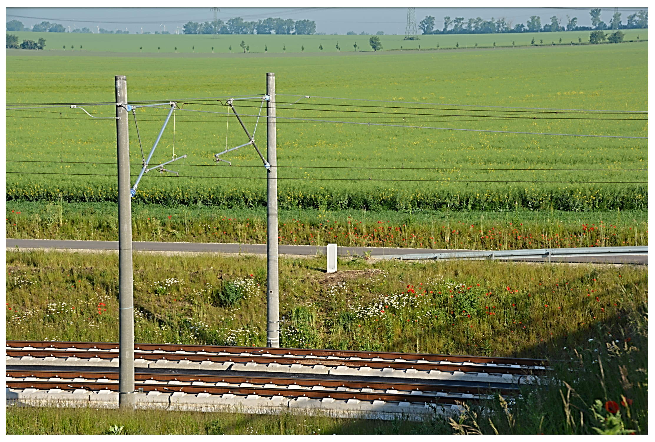
In this study, the catenary poles for high-speed rail routes, reaching a speed of 330 km/h−1, are chosen as a realistic case study, as shown in Figure 1. The poles are 10 m in height with tapered hollow circular sections and are produced by a spinning method. The outer diameter at the bottom end is 400 mm and reduces linearly to 250 mm at the top of the pole. The poles are embedded in typical pile foundations for a depth of 500 mm. Each pile foundation is constructed in a diameter of 500 mm and 5500 mm in depth. The foundations have a relatively high rigidity to minimize the soil–structure interaction and ensure the minimal structural and dynamic deformations of the poles. This minimizes the oscillation of the poles and the attached catenary system during and after the train passing.
The poles are made of a high-strength concrete with grade C80/95. Furthermore, the cross-section incorporates ten strands (7/, St 1680/1880), pre-stressed initially with a total force of approximately 680 KN. The strands are distributed equally throughout the perimeter. There is no additional longitudinal reinforcement, except two bars (Ø10 mm) used for grounding. Spiral reinforcement, with a diameter of 5 mm and pitch of 50 mm, is added along the pole. Further details about the geometry and materials of the poles can be found in [59].
Three of the catenary poles along a train track were provided with a monitoring system that consists of different types of sensors, mainly strains gauges and accelerometers. The behavior of the poles on site was investigated over a period of five years. It is shown that the poles on-site are still intact, and at least the first four modes are excited due to the ambient vibrations, namely, the wind and train passage [60]. However, these verifications are not within the scope of this study.
2.1. Simulation of Damaged Pole
To maintain the operation and the integrity of the monitored train system, introducing artificial damage to the poles in-service was impossible. Therefore, the behavior of the damaged poles was studied using FEM simulations by generating different expected damage scenarios. The poles of interest are numerically simulated using a 3D fully-detailed FEM model. The concrete material is simulated using solid elements with eight nodes, each with three degrees of freedom.
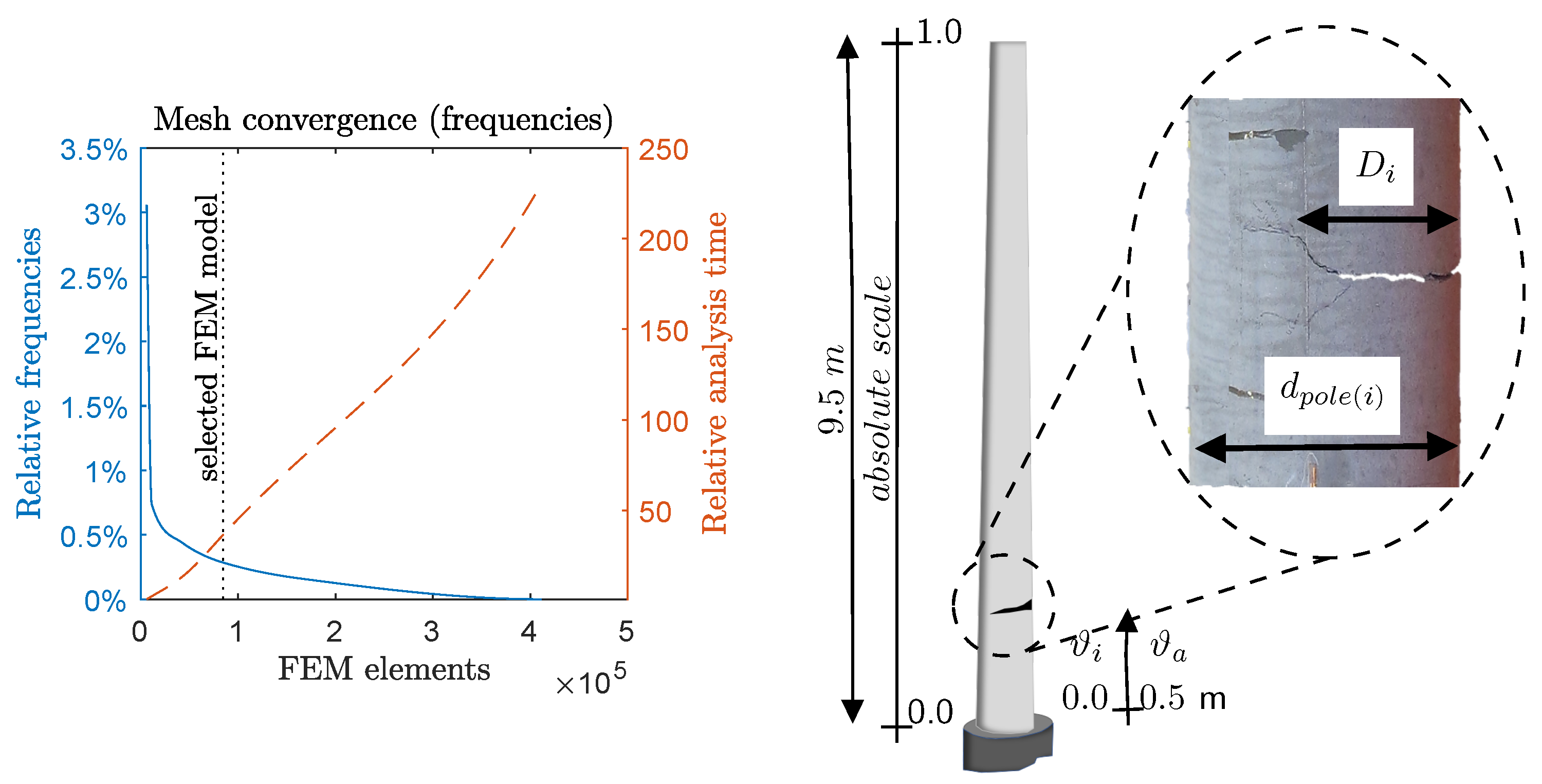
A convergence analysis shown inFigure 2 (left) was conducted to choose the sizes of finite elements and to balance between the precision of the results and analysis time, and to assure that the mesh size has no significant effect on the FEM results [61]. Consequently, the concrete material was simulated using solid elements with eight nodes, each with three degrees of freedom. The sizes of solid elements are approximately 50 × 50 × 25 mm in the longitudinal, circumferential, and radial directions, respectively.
Furthermore, the prestressing strands are simulated using 3D truss elements with two nodes and three degrees of freedom at each node. The prestressing forces are guaranteed by introducing initial strains to the truss elements of the model at the first step of analysis. In addition, linear material constitutive models are used to describe the behavior of concrete and prestressing strands for the conducted modal analysis of simulated poles. The contact between concrete and prestressing strands in the FEM model are considered monolithic. The boundary conditions are selected in accordance with the poles on-site, i.e., to represent the cantilever behavior of the pole.
Cracks (local damages) at specific locations along the pole are introduced by reducing the concrete modulus of elasticity at the crack location , as shown in Figure 2 (right). To ensure that the considered approach simulates relatively the real behavior of cracked poles, the numerical model is validated using experiments conducted on cracked poles. The validation process includes, but is not limited to, validating mode shapes, eigenfrequencies, and modal curvatures. However, this might add some uncertainty to the damage identification process, but it does not significantly impact the final results. More details about the conducted tests are available in [58]. The severity ratio of damage is defined, such as
where is the depth of the crack, and is the diameter of the cross-section at the damage location .
Local damages are repeated at absolute heights, measured from the bottom of the pole, as follows: with intervals of , and with intervals of . At each local damage point , five damage severity ratios are used. For a better interpretation of the results, the damage locations are normalized in the range of [0–1]. The normalized dimensionless damage locations are denoted as in the rest of this work.
2.2. Damage Features
The eigenfrequencies of studied poles are derived based on modal analysis of the FEM model, described in Section 2.1. The relative changes in eigenfrequencies of different modes are defined, as follows:
where and represent the eigenfrequencies of the ith mode of the damaged and un-damaged pole, respectively. Figure 3 represents the derived relation between normalized damage location , damage severity , and relative changes in eigenfrequencies of the first four modes. The surfaces in Figure 3 form vital damage features when used in conjunction with the Bayesian data fusion concept to identify the given structure’s damage. As known, the mode shape is not sensitive to damage when the damage is located near the nodes of the mode shape. Similarly, this means that some surfaces are more pertinent to detecting damage at a specific location than others.
Unlike the available literature, this study solved the problem of damage identification by providing a new application of the concept of data fusion (implicitly provided in Bayesian inference) through merging informative data from multiple surfaces of different mode shapes. The derived damage features provide an excellent candidate for building a damage detection algorithm that can detect the location and severity of damage along the pole based on the spatial characteristic of the derived changes in eigenfrequencies , shown in Figure 3.
3. Methodology
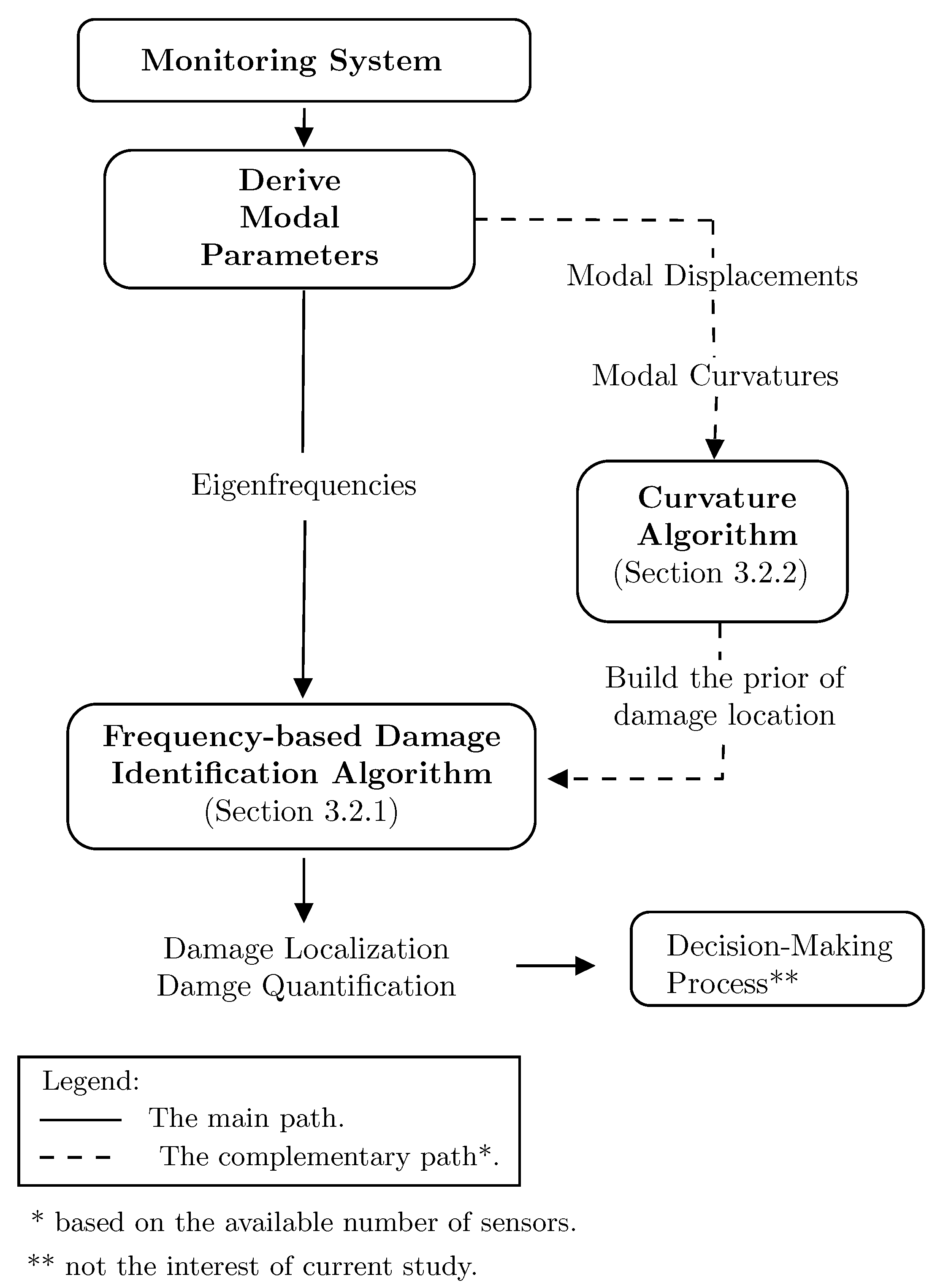
The proposed approach of damage identification is shown in Figure 4. Both damage location and damage severity are identified using the damage features derived in Section 2.2. In this sense, two vibration-based algorithms are proposed.
The main algorithm is the frequency-based damage identification (FDI) algorithm that detects the location and severity of the damage to Level 3 using the Bayesian inference and realizations of multiple damage features, namely, changes of the eigenfrequencies . One advantage of the Bayesian inference is that the UQ of the parameters of interest was integrated in this process [62]. Besides, the Bayesian inference is an efficient tool for data fusion, namely, using the joint occurrence of multiple phenomena [63].
In addition, this study considers the use of a complementary curvature-based damage identification (CDI) algorithm. The CDI algorithm localizes the damage along the structure using the modal curvatures as a damage feature. The implementation of the CDI algorithm required an excessive number of accelerometers (four at least) compared with the FDI algorithm. When available, the CDI algorithm can be integrated into the FDI algorithm as an informative prior.
3.1. Bayesian Inverse Problems
Given a forward model , the input parameters are mapped to the measured outputs through an operator , such that:
Defining the total prediction error as the discrepancy between the `real’ observations of the given system and both the model prediction and measurands [47,64], the measured observation is written, such as . The input parameters are divided, based on their uncertainty, into: input parameters subjected to uncertainty ; and well-known deterministic input parameters, [58].
The Bayesian approach uses the stochastic model of Equation (3) such that for solving inverse problems [38]. In inverse problems, the unknown input parameter is a random variable with a prior density . The prior density represents the belief about prior to measurements [65]. In addition, the observations are considered as a random variable that follows the probability distribution that has a PDF and realizations observed directly from measurements.
The total error is considered as a random variable with an appropriate density [66]. Considering as mutually independent of , the Bayes’ theorem is written such that [67]:
Using the concept of frequency-based damage identification (FDI), the likelihood is written, such that, ; in other words , where is the likelihood function [68].
The evidence is independent of and is considered as a normalization constant z [69].
As a result, the posterior in Equation (4) is written as a statement of proportionality, such as . The posterior density represents the solution of the inverse problem in the Bayesian inference. Different algorithms have been developed to evaluate the posterior and avoid the complexity of the analytical solution, such as using stochastic sampling Monte Carlo integration, and importance sampling [70]. Practically, the Markov chain Monte Carlo (MCMC) algorithms are used for drawing the parameter distributions from the posterior [71]. In the cases where the interest is only in estimating the statistical moments, the maximum a posteriori (MAP) estimator is utilized. The MAP represents the values of inferred parameters with the highest probabilities of occurrence, without the need to calculate the normalization factor z [72], such that:
3.2. Bayesian Damage Identification Algorithms
3.2.1. Frequency-Based Damage Identification Algorithm
A newly proposed FDI algorithm extends solving the DD problem in Levels 2 and 3 using a UQ framework. The FDI algorithm is a vibration-based Bayesian algorithm that fuses the informative data of multiple eigenfrequencies to localize and quantify the damage along the given structure.
The Bayesian approach illustrated in Section 3.1 is used to infer the unknowns of DD. Using the changes of the eigenfrequency as a damage feature, the realizations of observations are built, as follows, , where is the relative changes in the eigenfrequency of the ith mode, and n is the number of considered modes, as defined in Equation (2). The characteristics of the damage, that is, the damage location and damage severity , are considered as unknown parameters , such as .
The likelihood utilizes the concept of Bayesian data fusion to combine the damage information (shown in Figure 3) of multiple mode shapes. For mutually independent observations , the likelihood is written as , where represents the symmetric and positive-semidefinite covariance matrix. Consequently, the likelihood can be calculated such as
with being the ith component of the main diagonal of the matrix . For uncorrelated errors, the covariance matrix is rephrased to be , where is the variance of the errors. Considering the total errors to have a likely multivariate Gaussian distribution with zero-means . In this case, it is more convenient to use matrix notation in presenting the Gaussian multivariate likelihood, as follows:
The posterior in Equation (4) is updated as follows:
Accordingly, the unknown parameters can be inferred by sampling from the posterior using, for example, an MCMC algorithm.
The implementation of the FDI algorithm can be found in Section 4.2. The FDI algorithm works well using un-informative priors of the damage location and severity, for example, uniform probability distributions . However, an informative prior of damage location can be derived using the complementary curvature algorithm CDI (see Section 3.2.2).
3.2.2. Curvature-Based Damage Identification Algorithm
The CDI algorithm uses relative changes of modal curvatures to localize damages along the given structure by applying Bayesian inference techniques, as discussed in Section 3.1. Realizations of observations are considered such that , where is the modal curvature of the mode , and n is the number of considered mode shapes [73].
Unknown parameters vector is formed from the coordinates of the attached sensors m along the structure, such as . Optimal sensor location and number can be verified intensively using, for example, methodologies based on Fisher information matrix and information entropy [64]. However, this is out of the scope of the current study.
The concept of data fusion is implemented using Bayes theorem by structuring the likelihoods of various values of the unknowns given information obtained from multiple measurements . For mutually independent observations , the likelihood at location is written, such that:
with . The probability function is defined, as follows:
The absolute relative changes in the modal curvature are defined, such that , where and denote the un-damaged and damaged modal curvature of the mode at coordinate along the structure.
The prior is selected to decrease the probability gradually with an increase in the coordinate of the sensor . The selected prior fulfills the high probability of expected damage at the lower part of the cantilever structure, that is, at the points of high stress under applied actions.
Consequently, the posterior in Equation (4) is updated as follows:
using the concept of data fusion and the likelihood definition from Equation (9), the probability of damage at given the modal curvatures is written as
The identified damage locations using the CDI algorithm were discretized according to locations of available accelerometers. Therefore, the histograms derived from Equation (11) can be fitted and normalized to build continuous PDFs of informative priors for the implementation of the FDI algorithm.
While it is possible to obtain the eigenfrequencies using a simple signal processing method, it is necessary to use more complicated methods to derive the modal curvatures. In this study, the modal displacements of the given structure are derived using an output-only operational modal analysis, namely, the stochastic subspace identification (SSI) method (refer to [74] for more details). Then, having an array of sensors attached to the structure of interest at equally-distributed spaces , the modal curvature at coordinate j is numerically estimated using the second-order central difference approximation [75], as follows:
where , and are the measured modal displacements at three subsequent sensors.
4. Results
4.1. Implementation of Damage Identification Algorithms
In the absence of any data on the damaged poles in service, artificial measurements are generated using the FEM simulation mentioned in Section 2.1. To implement the complementary CDI algorithm, the locations of the sensors are chosen to be equally distributed along the pole using distances of mm, corresponding to the normalized dimensionless distances of .
The artificial measurements are created using combinations of damage location , damage severity (see, Section 2.1), and distances between sensors. The artificial modal curvatures and eigenfrequencies are perturbed using Gaussian noise with coefficients of variation of , and in addition to a bias of of the no-noise values. In total, 1500 records of artificial measurements were generated and utilized for implementing the proposed damage identification algorithms. Both the CDI and FDI algorithms are applied using the first four mode shapes and corresponding eigenfrequencies. For the easy interpretation of results, normalized dimensionless damage location in the range [0–1] is used.
4.2. Implementation of the Frequency-Based Damage Identification Algorithm
The FDI algorithm was implemented using the artificial measurements and the findings of the CDI algorithm as informative priors to damage locations . Uninformative priors of damage severity were used, such that . The posteriors were derived by implementing the MCMC algorithm [76] for 1000 samples.
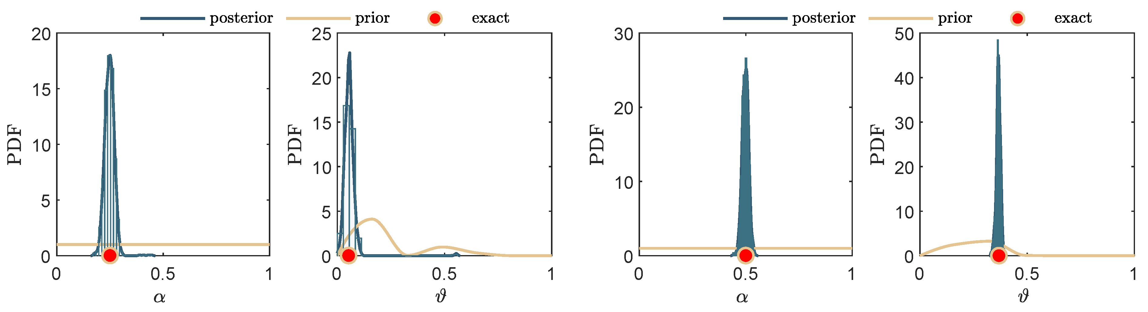
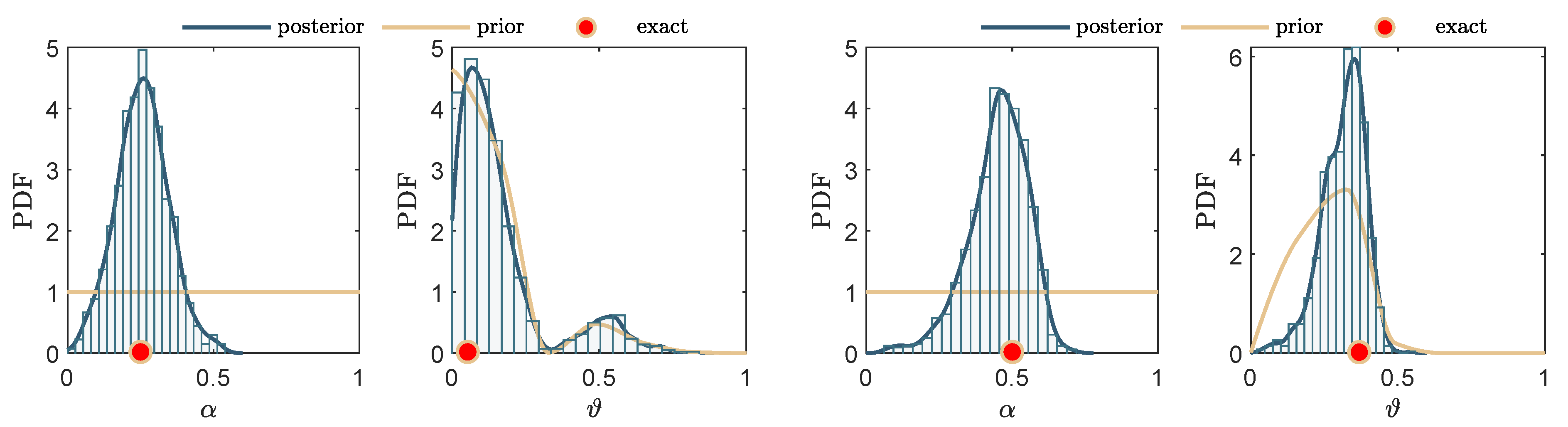
Some selected results of the FDI algorithm are depicted in Figure 5 and Figure 6, for noise levels of 1 and , respectively. The posteriors of the identified location and the identified severity are shown for selected damages at different locations and severities.
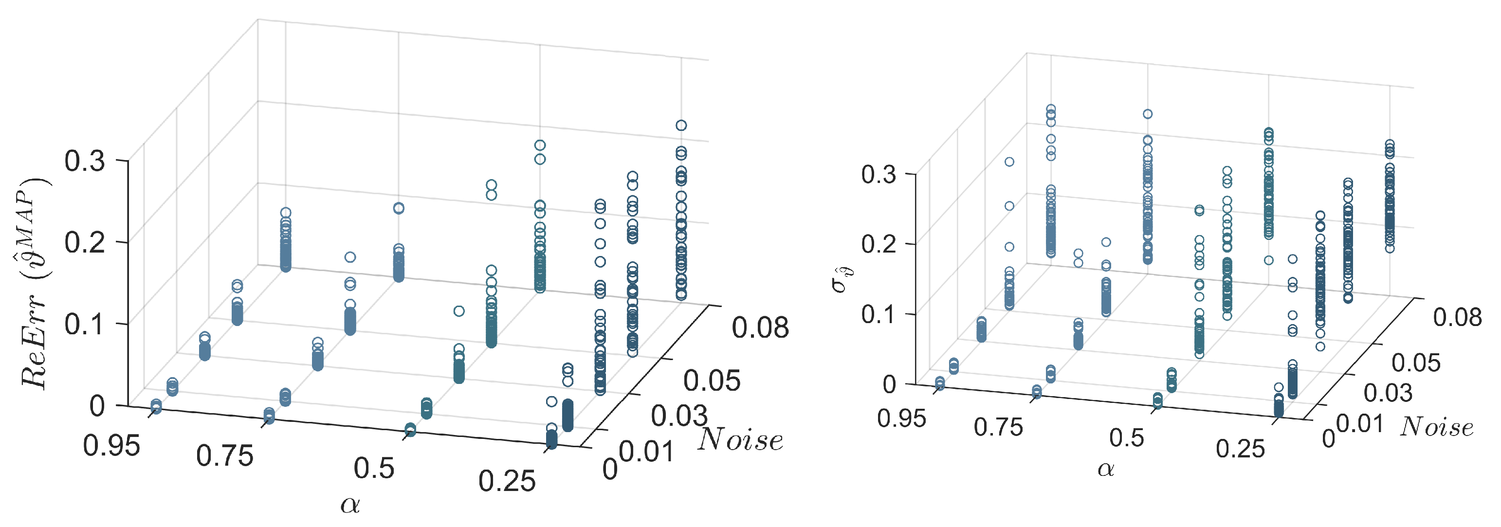
To evaluate the efficiency of the FDI, the re-constructed errors (ReErr) are calculated using 1500 records of artificial measurements. The ReErr is defined as the absolute difference between the artificial damage and MAP values of the identified damage characteristics; that is, (. The precision of the results is measured by the standard deviations of the posteriors; that is, (.
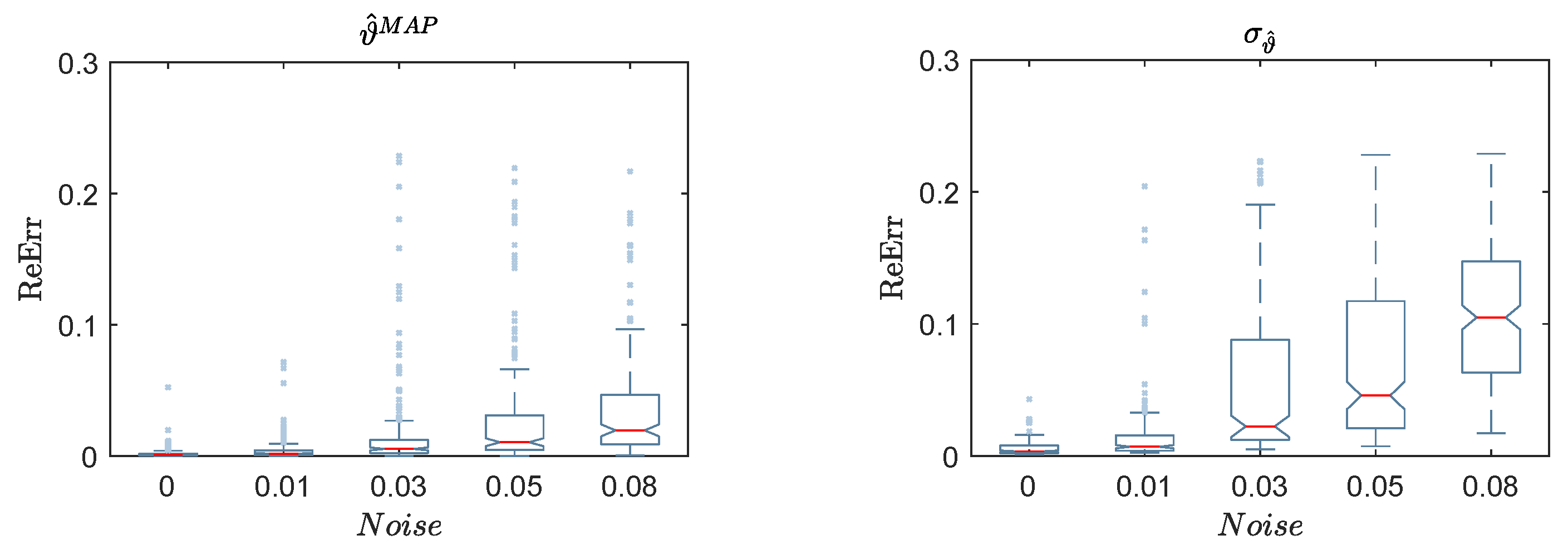
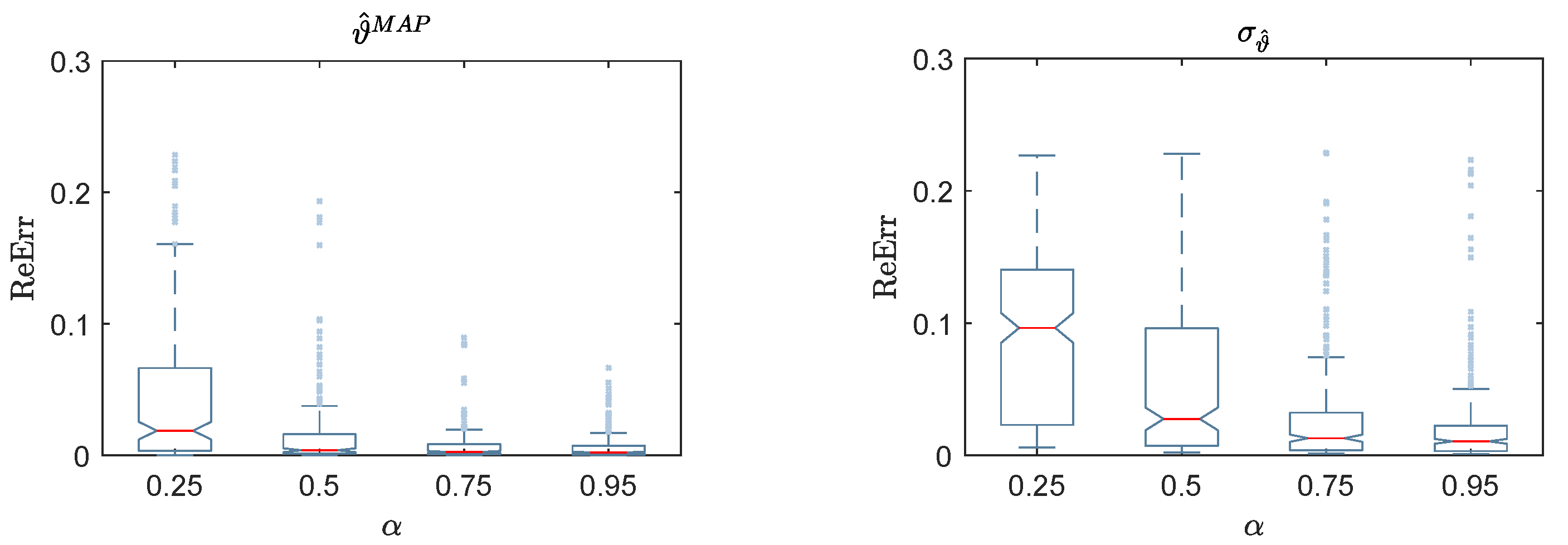
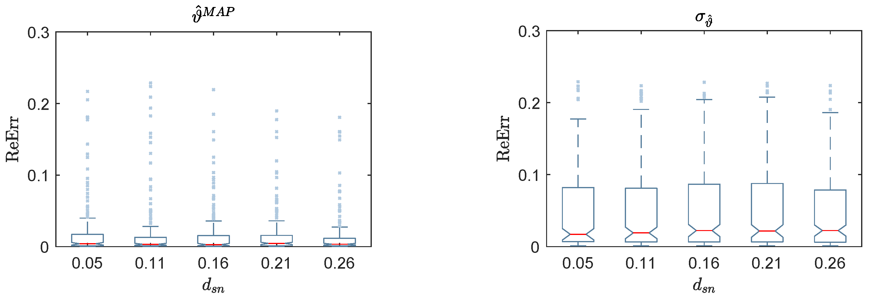
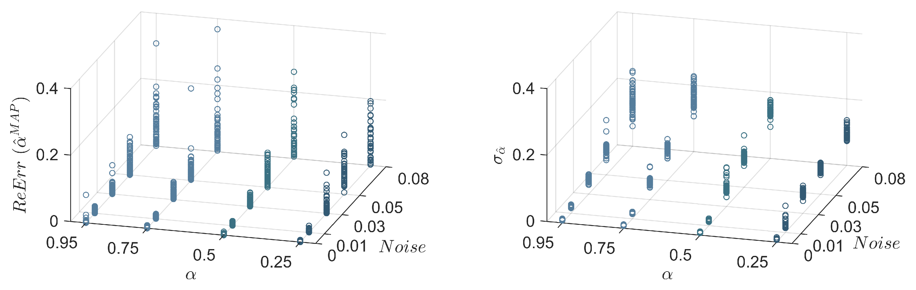
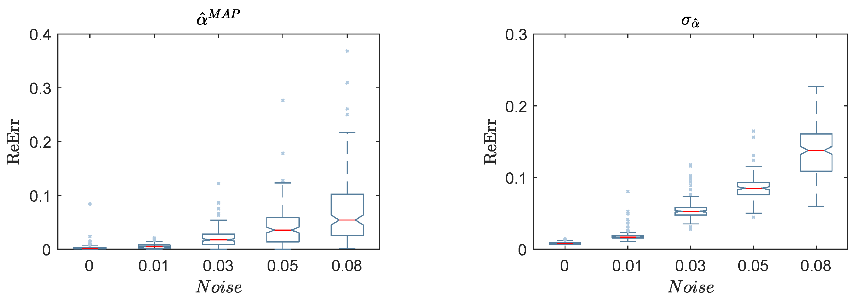
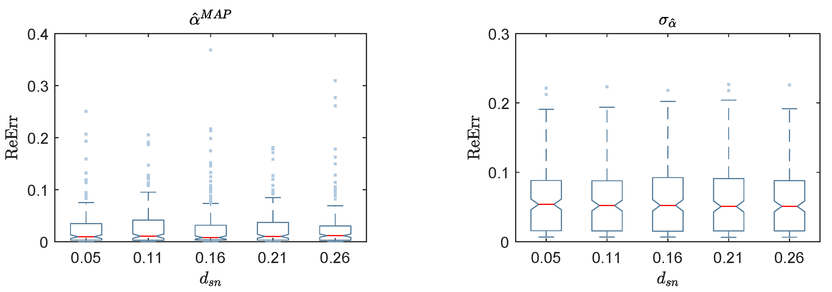
The and their are shown in Figure 7 for of . For a better interpretation of the results, standard box-plots are used to evaluate the statistical properties of the at each pair of noise levels and damage severity . For greater clarity, the box-plots are classified based on noise level, , and , as shown in Figure 8, Figure 9 and Figure 10 for the of . The and their of the are shown in Figure 11. In addition, the box-plots in Figure 12, Figure 13 and Figure 14 represent the of .
4.3. Implementation of the Curvature-Based Damage Identification Algorithm
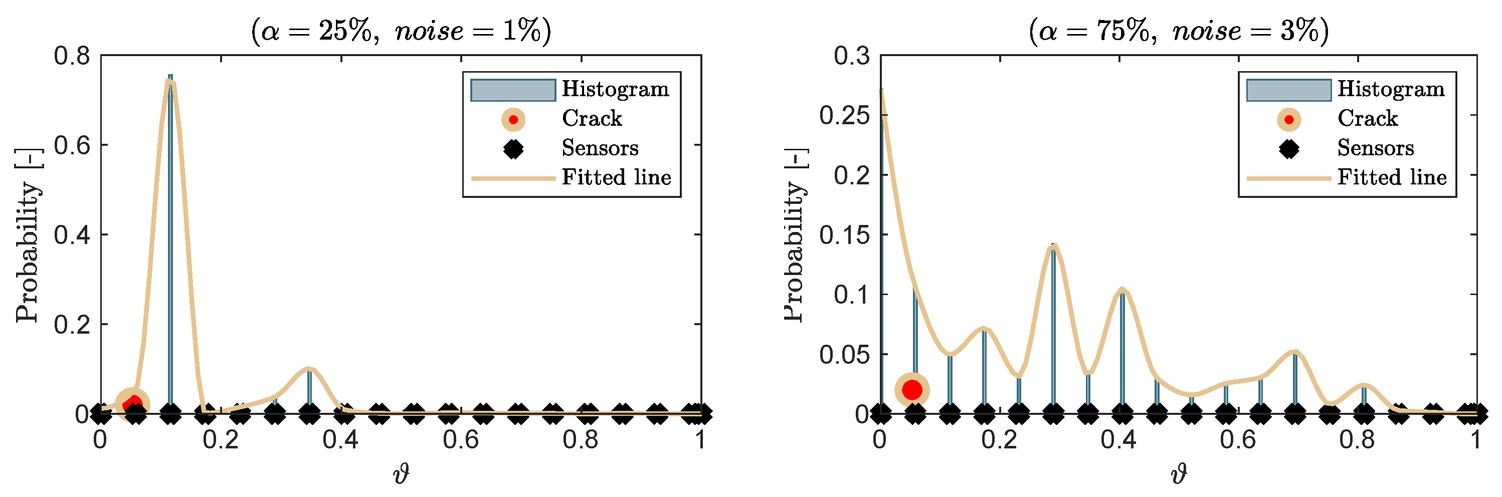
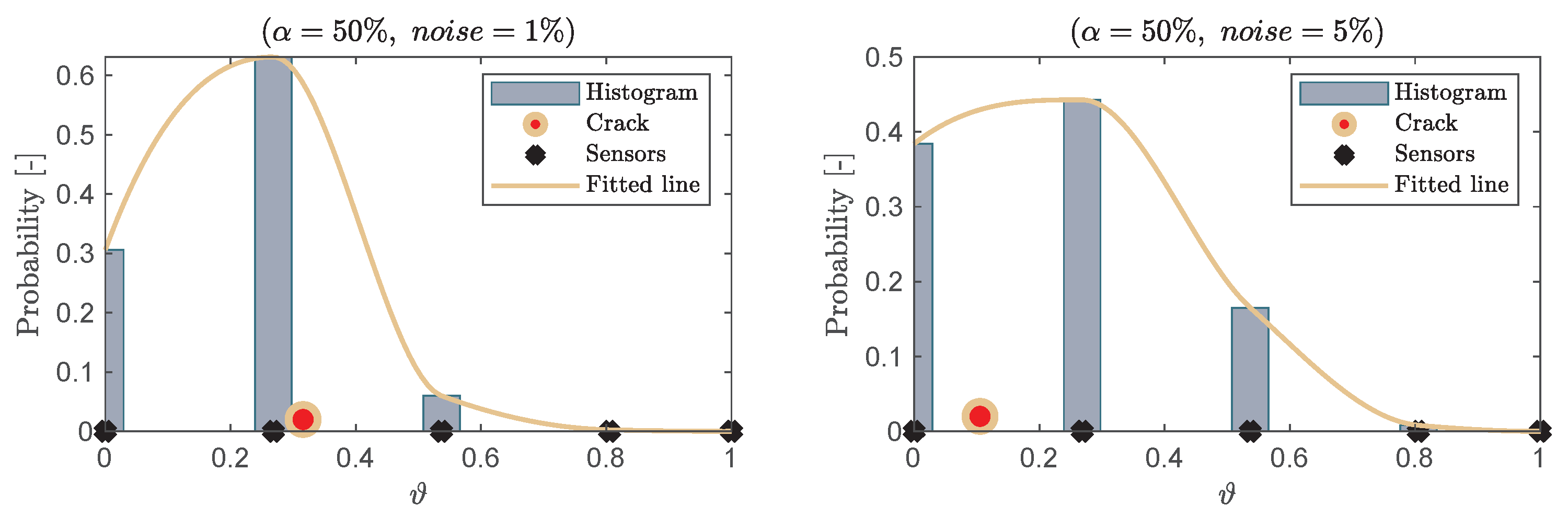
By implementing the CDI algorithm, it is noted that its accuracy is sensitive to the damage severity , noise level, and distance between the damage location and adjacent sensor. Several sensor arrangements are used in the following to study the efficiency of CDI. Examples of implementing this algorithm using artificial measurements and selected arrangements of sensors are shown in Figure 15 and Figure 16. The histograms and fitted lines present the probability of the damage location along the pole.
5. Discussion
5.1. Discussion of the Frequency-Based Damage Identification Algorithm
The results, depicted in Figure 5 and Figure 6, show the efficiency of the FDI algorithm in identifying the damage characteristics. It is evident that the exact damage location and damage severity coincide with the MAP values calculated using the FDI algorithm, even when using different noise levels up to . However, the noise level significantly affects the variances of the identified damage parameters, for example, for the identified damage location the variance, which changed from for the noise level of to for the noise level of , which is expected.
Furthermore, as shown in Figure 7 (left), the of identified damage location increases by increasing the noise level, and decreases by increasing damage severity , which is reasonable. It is evident that the efficiency of the FDI algorithm increases starting from damage severity , for example, at a noise level of the is for damage severity , and decreases to for damage severity . The standard deviations of the identified damage location , shown in Figure 7 (right), follows the same trend; however, these are more affected by the noise levels even for the cases of high damage severity, for example, .
The box-plots in Figure 8 provide a more accurate representation of the effect of the noise level on the of . The maximum values of reach for the noise level of with a maximum standard deviation of . In contrast, the in Figure 9 reaches a maximum value of at low damage severity , and decreases dramatically for damage severity from to . The same was concluded for the corresponding standard deviations, which touch the maximum value of at damage severity . The results in Figure 10 fluctuate around the converged values with a simple preference for the cases of , considering the values of the of and their . However, outliers can be seen in the box-plots that count less than of the verified data, according to the definition of standard box-plots. Then, they have no significant effects on the efficiency of the current results.
The of identified damage severity shown in Figure 11 follows the same trend, as in the case of . It is noted from Figure 11 (right) that the standard deviations are less scattered compared with similar cases of . Unlike the , the of identified damage severity is more sensitive to the level of noise than the damage severity. It reaches a maximum value of at a noise level of (see Figure 12), in comparison with at a damage severity of , as shown in Figure 13. The effects of on the of identified damage severity are similar to those of the of identified damage severity described previously, as shown in Figure 14.
In conclusion, the FDI algorithm is able to identify the location and the severity of the damage to an acceptable maximum error of at a noise level of . It should be kept in mind that the maximum values of the standard box-plots correspond to a probability of at the tails of the probability distribution of data. This means that is localized within a maximum error of 1150 mm, and is quantified with a maximum offset of from real damage severity.
5.2. Discussion of the Curvature-Based Damage Identification Algorithm
The algorithm provides a higher probability to the points around the damage location, which makes it a good prior for localizing the damage. However, it is evident that for distances between sensors of = [2000–2500] mm, more informative priors are achieved (even with high noise level) compared with the cases of smaller distances between sensors.
The efficiency of the CDI algorithm is based on the number of sensors, distances between sensors, and the accuracy of calculated modal curvatures. Therefore, it is noted that the damage was localized accurately when the damage was close to one of the sensors (see, for example, Figure 15). However, the CDI algorithm provides an informative prior that could be used in conjunction with other damage detection algorithms to localize the damage precisely; for example, using the normalized fitted lines in Figure 15 and Figure 16 as an informative prior.
6. Conclusions
In this study, a stochastic damage identification approach based on changes of eigenfrequencies of cantilever structures was proposed. The proposed algorithm was verified using catenary poles of electrified railways track. The characteristics of damaged structures due to local damage were artificially introduced by reducing the modulus of elasticity at the damage location. Different damage severities and damage locations were used to extract damage features of the structure of interest. Based on the findings of this study, several conclusions can be drawn as follows:
- The proposed damage features overcome the limitation of frequency-based damage identification methods available in the literature, which are valid to detect damage in structures to Level 1 only. It is enough to use the changes of the eigenfrequencies of cantilever structures to identify possible local damage at Level 3, i.e., to cover processes of damage detection, localization, and quantification. The FDI algorithm identified the damage with relatively small errors, even at a high noise level. Furthermore, the measurements needed to apply the proposed algorithm in practice which can be retrieved using fewer accelerometers compared with other available approaches described in the literature.
- Using the modal curvatures as a damage feature is very efficient for damage localization. This is shown from the results of the proposed CDI algorithm, as it offered a higher probability to the points around the damage location. Implementing this algorithm in practical cases needs more sensors (for example, at least four sensors) compared to the FDI algorithm, which might make it an unfeasible choice for the vast number of structures, as in catenary poles. However, the algorithm presented a significant accuracy, which made it a suitable prior to localizing the damage, even with a high noise level when a sufficient number of sensors are available.
- Bayesian inference is the suitable approach in this instance, despite its heavy computations. Different data can be utilized, and at the same time, the uncertainty of different parameters can be considered. Furthermore, the Bayesian inference simplifies the implementation data fusion concept in merging the informative data from multiple sources and methods. This approach increases the quality and accuracy of the expected results, for example, when used in the proposed FDI and CDI algorithms, to fuse the damage features from several measurements. Another benefit of using the Bayesian inference is quantifying the uncertainty of results caused by different sources of data and methods without additional efforts.
- Applying the proposed approach looks very promising when applied to other types of cantilever structures, such as the poles supported the power transmission lines, antenna masts, chimneys, and wind turbines. In addition, the proposed approach needs to be applied in practice for damage identification on real structures. Efforts should be made in this direction.
Author Contributions
Methodology, F.A.; software and analysis, F.A.; writing—original draft preparation, F.A.; revised the work, T.L.; supervision, T.L.; All authors have read and agreed to the published version of the manuscript.
Funding
This research received no external funding.
Institutional Review Board Statement
Not applicable.
Informed Consent Statement
Not applicable.
Data Availability Statement
Not applicable.
Acknowledgments
This work was done under the support of the Deutsche Forschungsgemeinschaft (DFG) through the Research Training Group 1462, which is greatly acknowledged by the authors. Another acknowledgment goes to the German Academic Exchange Service (DAAD) for supporting the main author through the scholarship program “Leadership for Syria”.
Conflicts of Interest
The authors declare no conflict of interest.
Abbreviations
The following abbreviations are used in this manuscript:
| CDI | Curvature-Based Damage Identification |
| DD | Damage Detection |
| FDI | Frequency-Based Damage Identification |
| FEM | Finite Element Method |
| MAP | Maximum A Posteriori |
| MCMC | Markov Chain Monte Carlo |
| MLE | Maximum Likelihood Estimator |
| Probability Distribution Function | |
| ReErr | Reconstructed Error |
| SHM | Structural Health Monitoring |
| SI | System Identification |
| SSI | Stochastic Subspace Identification |
| UQ | Uncertainty Quantification |
References
- Farrar, C.R.; Worden, K. Structural Health Monitoring: A Machine Learning Perspective; John Wiley & Sons: Hoboken, NJ, USA, 2012. [Google Scholar] [CrossRef] [Green Version]
- Goulet, J.A.; Der Kiureghian, A.; Li, B. Pre-posterior optimization of sequence of measurement and intervention actions under structural reliability constraint. Struct. Saf. 2015, 52, 1–9. [Google Scholar] [CrossRef] [Green Version]
- Song, G.; Wang, C.; Wang, B. Structural Health Monitoring (SHM) of Civil Structures; Multidisciplinary Digital Publishing Institute: Basel, Switzerland, 2017. [Google Scholar] [CrossRef]
- Zona, A. Vision-Based Vibration Monitoring of Structures and Infrastructures: An Overview of Recent Applications. Infrastructures 2021, 6, 4. [Google Scholar] [CrossRef]
- Doebling, S.; Farrar, C.; Prime, M.; Shevitz, D. Damage Identification and Health Monitoring of Structural and Mechanical Systems from Changes in Their Vibration Characteristics: A Literature Review. 1996. Available online: https://www.osti.gov/biblio/249299-damage-identification-health-monitoring-structural-mechanical-systems-from-changes-vibration-characteristics-literature-review (accessed on 21 March 2020). [CrossRef] [Green Version]
- Yan, J.X.; Liu, C.S.; Liu, T.Z.; Zhao, L.L. A review on advances of damage identification methods based on vibration. In Key Engineering Materials; Trans Tech Publications Ltd.: Stafa-Zurich, Switzerland, 2009; Volume 413, pp. 277–283. [Google Scholar] [CrossRef]
- An, Y.; Chatzi, E.; Sim, S.H.; Laflamme, S.; Blachowski, B.; Ou, J. Recent progress and future trends on damage identification methods for bridge structures. Struct. Control Health Monit. 2019, 26, e2416. [Google Scholar] [CrossRef]
- Rodgers, J.; Thomas, E. Prestressed Concrete Poles: State-of-the-Art. PCI J. 1984, 29, 52–103. [Google Scholar] [CrossRef]
- Fam, A. Development of a novel pole using spun-cast concrete inside glass-fiber-reinforced polymer tubes. PCI J. 2008, 53, 100–113. [Google Scholar] [CrossRef]
- Oliphant, W.J.; Sherman, D.C. Prestressed Concrete Transmission Pole Structures; American Society of Civil Engineers: Reston, VA, USA, 2012. [Google Scholar] [CrossRef]
- Kuebler, M.E. Torsion in Helically Reinforced Prestressed Concrete Poles. Master’s Thesis, University of Waterloo, Waterloo, ON, Canada, 2008. [Google Scholar]
- Kuebler, M.; Polak, M.A. Torsion tests on spun-cast prestressed concrete poles. PCI J. 2012, 57, 120–141. [Google Scholar] [CrossRef]
- PCI Committee on Prestressed Concrete Poles. Guide for the Design of Prestressed Concrete Poles. PCI J. 1997, 42, 94–137. [Google Scholar]
- DIN EN 12843:2004-11. Precast Concrete Products—Masts and Poles; German Version EN 12843:2004; Deutsche Institut für Normung e.V.: Berlin, Germany, 2004. [Google Scholar]
- Fouad, F.H.; Scott, N.L.; Calvert, E.; Donovan, M. Performance of spun prestressed concrete poles during Hurricane Andrew. PCI J. 1994, 39, 102–110. [Google Scholar] [CrossRef]
- Ibrahim, A.M. Behaviour of Pre-stressed Concrete Transmission Poles under High Intensity Wind. Ph.D. Thesis, University of Western Ontario, London, ON, Canada, 2017. [Google Scholar]
- Dilger, W.H.; Ghali, A.; Mohan Rao, S. Improving Durability And Performance Of Spun-Cast Concrete Poles. PCI J. 1996, 41, 68–90. [Google Scholar] [CrossRef]
- Remitz, J.; Wichert, M.; Empelmann, M. Ultra-High Performance Spun Concrete Poles—Part I: Load-bearing behaviour. In Proceedings of the HPC/CIC, Tromsö, Norway, 6–8 March 2017; p. 54. [Google Scholar]
- Wichert, M.; Remitz, J.; Empelmann, M. Ultra-High Performance Spun Concrete Poles—Part II: Tests on Grouted Pole Joints. In Proceedings of the HPC/CIC, Tromsö, Norway, 6–8 March 2017; p. 54. [Google Scholar]
- Chen, S.; Ong, C.K.; Antonsson, K. Modal behaviors of spun-cast pre-stressed concrete pole structures. In Proceedings of the IMAC–XXIV, St. Louis, MO, USA, 30 January–2 February 2006; pp. 1831–1836. [Google Scholar]
- Chen, S.E.; Dai, K. Modal characteristics of two operating power transmission poles. Shock Vib. 2010, 17, 551–561. [Google Scholar] [CrossRef]
- Dai, K.; Chen, S.; Smith, D. Vibration analyses of electrical transmission spun-cast concrete poles for health monitoring. In Nondestructive Characterization for Composite Materials, Aerospace Engineering, Civil Infrastructure, and Homeland Security 2012; International Society for Optics and Photonics: San Diego, CA, USA, 2012; Volume 8347, p. 834702. [Google Scholar]
- Abedin, M.; Mehrabi, A.B. Novel Approaches for Fracture Detection in Steel Girder Bridges. Infrastructures 2021, 4, 42. [Google Scholar] [CrossRef] [Green Version]
- Chang, P.C.; Flatau, A.; Liu, S. Health monitoring of civil infrastructure. Struct. Health Monit. 2003, 2, 257–267. [Google Scholar] [CrossRef]
- Balageas, D.; Fritzen, C.P.; Güemes, A. Structural Health Monitoring; John Wiley & Sons: Hoboken, NJ, USA, 2010; Volume 90. [Google Scholar] [CrossRef] [Green Version]
- Tangirala, A.K. Principles of System Identification: Theory and Practice; CRC Press: Boca Raton, FL, USA, 2014. [Google Scholar]
- Rytter, A. Vibrational Based Inspection of Civil Engineering Structures. Ph.D. Thesis, University of Aalborg, Aalborg, Denmark, 1993; 206p. [Google Scholar]
- Rajan, G.; Prusty, B.G. Structural Health Monitoring of Composite Structures Using Fiber Optic Methods; CRC Press: Boca Raton, FL, USA, 2016. [Google Scholar]
- Giordano, P.F.; Quqa, S.; Limongelli, M.P. Statistical Approach for Vibration-Based Damage Localization in Civil Infrastructures Using Smart Sensor Networks. Infrastructures 2021, 6, 22. [Google Scholar] [CrossRef]
- Sohn, H.; Farrar, C.R.; Hemez, F.M.; Czarnecki, J.J. A Review of Structural Health Review of Structural Health Monitoring Literature 1996–2001. 2002. Available online: https://www.osti.gov/biblio/976152 (accessed on 21 March 2020).
- Doebling, S.W.; Farrar, C.R.; Prime, M.B. A summary review of vibration-based damage identification methods. Shock Vib. Dig. 1998, 30, 91–105. [Google Scholar] [CrossRef] [Green Version]
- Moughty, J.J.; Casas, J.R. A state of the art review of modal-based damage detection in bridges: Development, challenges, and solutions. Appl. Sci. 2017, 7, 510. [Google Scholar] [CrossRef] [Green Version]
- Avci, O.; Abdeljaber, O.; Kiranyaz, S.; Hussein, M.; Gabbouj, M.; Inman, D.J. A review of vibration-based damage detection in civil structures: From traditional methods to Machine Learning and Deep Learning applications. Mech. Syst. Signal Process. 2021, 147, 107077. [Google Scholar] [CrossRef]
- Reynders, E.; De Roeck, G. Vibration-based damage identification: The z24 bridge benchmark. Encycl. Earthq. Eng. 2014, 482, 1–8. [Google Scholar] [CrossRef]
- Sha, G.; Radzieński, M.; Cao, M.; Ostachowicz, W. A novel method for single and multiple damage detection in beams using relative natural frequency changes. Mech. Syst. Signal Process. 2019, 132, 335–352. [Google Scholar] [CrossRef]
- Chen, H.P.; Ni, Y.Q. Structural Health Monitoring of Large Civil Engineering Structures; Wiley Online Library: Hoboken, NJ, USA, 2018. [Google Scholar]
- Alkam, F.; Lahmer, T. On the quality of identified parameters of prestressed concrete catenary poles in existence of uncertainty using experimental measurements and differenterent optimization methods. In Proceedings of the 28th International Conference on Noise and Vibration Engineering, ISMA 2018 and 7th International Conference on Uncertainty in Structural Dynamics, USD 2018, Leuven, Belgium, 17–19 September 2018; Desmet, W., Pluymers, B., Moens, D., Rottiers, W., Eds.; KU Leuven-Departement Werktuigkunde: Leuven, Belgium, 2018; pp. 3913–3923. [Google Scholar]
- Bigoni, D.; Engsig-Karup, A. Uncertainty Quantification with Applications to Engineering Problems; DTU Compute: Kongens Lyngby, Denmark, 2014. [Google Scholar]
- Li, B. Uncertainty Quantification in Vibration-Based Structural Health Monitoring Using Bayesian Statistics. Ph.D. Thesis, UC Berkeley, Berkeley, CA, USA, 2016. [Google Scholar]
- Simoen, E.; Lombaert, G. Bayesian Parameter Estimation. In Identification Methods for Structural Health Monitoring; Chatzi, E., Papadimitriou, C., Eds.; Springer: Cham, Switzerland, 2016; pp. 89–115. [Google Scholar] [CrossRef]
- Feng, Z.; Lin, Y.; Wang, W.; Hua, X.; Chen, Z. Probabilistic Updating of Structural Models for Damage Assessment Using Approximate Bayesian Computation. Sensors 2020, 20, 3197. [Google Scholar] [CrossRef]
- Au, S.K. Bayesian Operational Modal Analysis. In Identification Methods for Structural Health Monitoring; Chatzi, E., Papadimitriou, C., Eds.; Springer: Cham, Switzerland, 2016; pp. 117–135. [Google Scholar] [CrossRef]
- Chiachio, M.; Beck, J.L.; Chiachio, J.; Rus, G. Approximate Bayesian Computation by Subset Simulation. SIAM J. Sci. Comput. 2014, 36, A1339–A1358. [Google Scholar] [CrossRef] [Green Version]
- Vanik, M.W.; Beck, J.L.; Au, S.K. Bayesian probabilistic approach to structural health monitoring. J. Eng. Mech. 2000, 126, 738–745. [Google Scholar] [CrossRef] [Green Version]
- Papadimitriou, C. Bayesian Uncertainty Quantification and  Propagation: State-of-the-Art Tools for Linear and Nonlinear Structural Dynamics Models. In Identification Methods for Structural Health Monitoring; Chatzi, E., Papadimitriou, C., Eds.; Springer: Cham, Switzerland, 2016; pp. 137–170. [Google Scholar] [CrossRef]
- Ching, J.; Muto, M.; Beck, J.L. Structural model updating and health monitoring with incomplete modal data using Gibbs sampler. Comput. Aided Civ. Infrastruct. Eng. 2006, 21, 242–257. [Google Scholar] [CrossRef]
- Simoen, E.; Papadimitriou, C.; Lombaert, G. On prediction error correlation in Bayesian model updating. J. Sound Vib. 2013, 332, 4136–4152. [Google Scholar] [CrossRef]
- Huang, Y.; Shao, C.; Wu, B.; Beck, J.L.; Li, H. State-of-the-art review on Bayesian inference in structural system identification and damage assessment. Adv. Struct. Eng. 2019, 22, 1329–1351. [Google Scholar] [CrossRef]
- Liggins, M., II; Hall, D.; Llinas, J. Handbook of Multisensor Data Fusion: Theory and Practice; CRC Press: Boca Raton, FL, USA, 2001. [Google Scholar]
- Raol, J.R. Multi-Sensor Data Fusion with MATLAB; CRC Press: Boca Raton, FL, USA, 2009. [Google Scholar]
- Smyth, A.W.; Kontoroupi, T.; Brewick, P.T. Efficient Data Fusion and Practical Considerations for Structural Identification. In Identification Methods for Structural Health Monitoring; Chatzi, E., Papadimitriou, C., Eds.; Springer: Cham, Switzerland, 2016; pp. 35–49. [Google Scholar] [CrossRef]
- Guo, H. Structural damage detection using information fusion technique. Mech. Syst. Signal Process. 2006, 20, 1173–1188. [Google Scholar] [CrossRef]
- Bao, Y.; Xia, Y.; Li, H.; Xu, Y.L.; Zhang, P. Data fusion-based structural damage detection under varying temperature conditions. Int. J. Struct. Stab. Dyn. 2012, 12, 1250052. [Google Scholar] [CrossRef] [Green Version]
- Sha, G.; Cao, M.; Xu, W.; Novák, D. Structural damage identification using multiple mode fusion curvature mode shape method. Structural Health Monitoring and Integrity Management. In Proceedings of the 2nd International Conference of Structural Health Monitoring and Integrity Management (ICSHMIM 2014), Nanjing, China, 24–26 September 2014; CRC Press: Boca Raton, FL, USA, 2015; p. 163. [Google Scholar]
- Aster, R.C.; Borchers, B.; Thurber, C.H. Parameter Estimation and Inverse Problems, 2nd ed.; Academic Press: Cambridge, MA, USA, 2013. [Google Scholar] [CrossRef]
- Dashti, M.; Stuart, A.M. The Bayesian Approach to Inverse Problems. In Handbook of Uncertainty Quantification; Ghanem, R., Higdon, D., Owhadi, H., Eds.; Springer: Cham, Switzerland, 2017; pp. 311–428. [Google Scholar] [CrossRef] [Green Version]
- Tarantola, A. Inverse Problem Theory and Methods for Model Parameter Estimation; Society for Industrial and Applied Mathematics: Philadelphia, PA, USA, 2005. [Google Scholar] [CrossRef] [Green Version]
- Alkam, F.; Pereira, I.; Lahmer, T. Qualitatively-improved identified parameters of prestressed concrete catenary poles using sensitivity-based Bayesian approach. Results Eng. 2020, 6, 100104. [Google Scholar] [CrossRef]
- Alkam, F.; Lahmer, T. Quantifying the Uncertainty of Identificationed Parameters of Prestressed Concrete Poles Using the Experimental Measurements and Different Optimization Methods. Eng. Appl. Sci. 2019, 4, 84. [Google Scholar] [CrossRef]
- Göbel, L.; Mucha, F.; Jaouadi, Z.; Kavrakov, I.; Legatiuk, D.; Abrahamczyk, L.; Kraus, M.; Smarsly, K. Monitoring the Structural Response of Reinforced Concrete Poles Along High-Speed Railway Tracks. In Proceedings of the International RILEM Conference on Materials, Systems and Structures in Civil Engineering—Conference Segment on Reliability, Lyngby, Denmark, 15–29 August 2016; Technical University of Denmark Lyngby: Lynby, Denmark, 2016; pp. 1–10. [Google Scholar]
- Batikha, M.; Alkam, F. The Effect of Mechanical Properties of Masonry on the behavior of FRP-strengthened Masonry-infilled RC Frame under Cyclic Load. Compos. Struct. 2015, 134, 513–522. [Google Scholar] [CrossRef]
- Alkam, F.; Lahmer, T. Solving Non-Uniqueness Issues in Parameter Identification problems for Pre-stressed Concrete Poles by Multiple Bayesian updating. In Proceedings of the 15th International Probabilistic Workshop & 10th Dresdner Probabilistik Workshop, Dresden, Germany, 27–29 September 2017; Voigt, M.P., Ed.; TUD Press: Dresden, Germany, 2017; pp. 303–315. [Google Scholar]
- Goulet, J.A. Probabilistic Machine Learning for Civil Engineers; MIT Press: Cambridge, MA, USA, 2020. [Google Scholar]
- Reichert, I.; Olney, P.; Lahmer, T. Influence of the error description on model-based design of experiments. Eng. Struct. 2019, 193, 100–109. [Google Scholar] [CrossRef]
- Gelman, A.; Carlin, J.B.; Stern, H.S.; Rubin, D.B. Bayesian Data Analysis, 3rd ed.; Chapman & Hall/CRC: Boca Raton, FL, USA, 2014; Volume 2. [Google Scholar]
- Kaipio, J.; Somersalo, E. Statistical and Computational Inverse Problems; Springer: Berlin/Heidelberg, Germany, 2006; Volume 160. [Google Scholar]
- Calvetti, D.; Somersalo, E. An Introduction to Bayesian Scientific Computing: Ten Lectures on Subjective Computing; Springer: Berlin/Heidelberg, Germany, 2007; Volume 2. [Google Scholar] [CrossRef]
- Stuart, A.M. Inverse problems: A Bayesian perspective. Acta Numer. 2010, 19, 451–559. [Google Scholar] [CrossRef] [Green Version]
- Idier, J. Bayesian Approach to Inverse Problems; John Wiley & Sons: Hoboken, NJ, USA, 2013. [Google Scholar]
- Bishop, C.M. Pattern Recognition and Machine Learning (Information Science and Statistics); Springer: Berlin/Heidelberg, Germany, 2006. [Google Scholar]
- Marzouk, Y.M.; Najm, H.N.; Rahn, L.A. Stochastic Spectral Methods for Efficient Bayesian Solution of Inverse Problems. J. Comput. Phys. 2007, 224, 560–586. [Google Scholar] [CrossRef]
- Bailer-Jones, C.A.L. Practical Bayesian Inference: A Primer for Physical Scientists; Cambridge University Press: Cambridge, UK, 2017. [Google Scholar] [CrossRef]
- Liggins, M.; Hall, D.; Llinas, J. Handbook of Multisensor Data Fusion: Theory and Practice, Second Edition; Electrical Engineering & Applied Signal Processing Series; Taylor & Francis: Abingdon, UK, 2008. [Google Scholar]
- Reynders, E.; Maes, K.; Lombaert, G.; De Roeck, G. Uncertainty quantification in operational modal analysis with stochastic subspace identification: Validation and applications. Mech. Syst. Signal Process. 2016, 66, 13–30. [Google Scholar] [CrossRef]
- Pandey, A.; Biswas, M.; Samman, M. Damage detection from changes in curvature mode shapes. J. Sound Vib. 1991, 145, 321–332. [Google Scholar] [CrossRef]
- Betz, W.; Papaioannou, I.; Straub, D. Transitional Markov Chain Monte Carlo: Observations and improvements. J. Eng. Mech. 2016, 142, 04016016. [Google Scholar] [CrossRef] [Green Version]
Figure 1.
The catenary pole system for high-speed rail routes.

Figure 2.
FEM mesh convergence analysis (left), and a description of the local damage (right).

Figure 3.
Relative changes of eigenfrequencies for the [1st–4th] modes, calculated for different values of damage severity , and normalized damage location .
Figure 3.
Relative changes of eigenfrequencies for the [1st–4th] modes, calculated for different values of damage severity , and normalized damage location .

Figure 4.
The flow chart of the proposed approach.

Figure 5.
Identified damage severity , and damage location , using the frequency-based algorithm for : , and (left); , and (right).
Figure 5.
Identified damage severity , and damage location , using the frequency-based algorithm for : , and (left); , and (right).

Figure 6.
Identified damage severity , and damage location , using the frequency-based algorithm for : , and (left); , and (right).
Figure 6.
Identified damage severity , and damage location , using the frequency-based algorithm for : , and (left); , and (right).

Figure 7.
Reconstructed error (ReErr) of the identified damage location using the frequency-based algorithm: the maximum a posteriori (MAP) values (left); and the standard deviation (right).
Figure 7.
Reconstructed error (ReErr) of the identified damage location using the frequency-based algorithm: the maximum a posteriori (MAP) values (left); and the standard deviation (right).

Figure 8.
Box-plot of the reconstructed error (ReErr) of the identified damage location , classified based on noise level: the MAP values (left); and the standard deviation (right).
Figure 8.
Box-plot of the reconstructed error (ReErr) of the identified damage location , classified based on noise level: the MAP values (left); and the standard deviation (right).

Figure 9.
Box-plot of the reconstructed error (ReErr) of the identified damage location , classified based on damage severity: the MAP values (left); and the standard deviation (right).
Figure 9.
Box-plot of the reconstructed error (ReErr) of the identified damage location , classified based on damage severity: the MAP values (left); and the standard deviation (right).

Figure 10.
Box-plot of the reconstructed error (ReErr) of the identified damage location , classified based on the distances between sensors : the MAP values (left); and the standard deviation (right).
Figure 10.
Box-plot of the reconstructed error (ReErr) of the identified damage location , classified based on the distances between sensors : the MAP values (left); and the standard deviation (right).

Figure 11.
Reconstructed error (ReErr) of the identified damage severity using the frequency-based algorithm: the MAP values (left); and the standard deviation (right).
Figure 11.
Reconstructed error (ReErr) of the identified damage severity using the frequency-based algorithm: the MAP values (left); and the standard deviation (right).

Figure 12.
Box-plot of the reconstructed error (ReErr) of the identified damage location , classified based on noise level: the MAP values (left); and the standard deviation (right).
Figure 12.
Box-plot of the reconstructed error (ReErr) of the identified damage location , classified based on noise level: the MAP values (left); and the standard deviation (right).

Figure 13.
Box-plot of the reconstructed error (ReErr) of the identified damage location , classified based on damage severity: the MAP values (left); and the standard deviation (right).
Figure 13.
Box-plot of the reconstructed error (ReErr) of the identified damage location , classified based on damage severity: the MAP values (left); and the standard deviation (right).

Figure 14.
Box-plot of the reconstructed error (ReErr) of the identified damage location , classified based on the distances between sensors : the MAP values (left); and the standard deviation (right).
Figure 14.
Box-plot of the reconstructed error (ReErr) of the identified damage location , classified based on the distances between sensors : the MAP values (left); and the standard deviation (right).

Figure 15.
Localizing the damage using the curvature algorithm: for , , , and (left); for , , , and (right).
Figure 15.
Localizing the damage using the curvature algorithm: for , , , and (left); for , , , and (right).

Figure 16.
Localizing the damage using the curvature algorithm: for , , , and (left); for , , , and (right).
Figure 16.
Localizing the damage using the curvature algorithm: for , , , and (left); for , , , and (right).

Publisher’s Note: MDPI stays neutral with regard to jurisdictional claims in published maps and institutional affiliations. |
© 2021 by the authors. Licensee MDPI, Basel, Switzerland. This article is an open access article distributed under the terms and conditions of the Creative Commons Attribution (CC BY) license (https://creativecommons.org/licenses/by/4.0/).
Share and Cite
MDPI and ACS Style
Alkam, F.; Lahmer, T. Eigenfrequency-Based Bayesian Approach for Damage Identification in Catenary Poles. Infrastructures 2021, 6, 57. https://0-doi-org.brum.beds.ac.uk/10.3390/infrastructures6040057
AMA Style
Alkam F, Lahmer T. Eigenfrequency-Based Bayesian Approach for Damage Identification in Catenary Poles. Infrastructures. 2021; 6(4):57. https://0-doi-org.brum.beds.ac.uk/10.3390/infrastructures6040057
Chicago/Turabian StyleAlkam, Feras, and Tom Lahmer. 2021. "Eigenfrequency-Based Bayesian Approach for Damage Identification in Catenary Poles" Infrastructures 6, no. 4: 57. https://0-doi-org.brum.beds.ac.uk/10.3390/infrastructures6040057