Numerical Modelling and Experimental Testing of the Hydrodynamic Characteristics for an Open-Frame Remotely Operated Vehicle

Abstract

The remotely operated vehicles (ROVs) are important to provide the technology support for both the traditional offshore structures and rapidly-growing renewable energy facilities during their full-lifecycles, such as site survey, installation, inspection, maintenance and repair. Regarding the motion and performance of a ROV, the understanding of its hydrodynamic properties is essential when exposing to the disturbances of wave and current. In this study, a numerical model is proposed within the frame of an open-source platform OpenFOAM. The hydrodynamics of the adopted ROV (BlueRov2) in its four principal degrees of freedoms (DOFs) is numerically simulated by a Reynolds-Averaged Navier-Stokes (RANS) solver. Meanwhile, an experimental test is carried out by using a novel technique on measuring the hydrodynamic forces and moments. To validate the numerical prediction methodologies, a set of systematic simulations of the ROV subjected to the disturbances caused by various flow conditions are performed. Comparing to the model test measurement, the numerical model proved to be reliable in offering a good estimation of the hydrodynamic parameters. This also indicates that the presented numerical methodologies and experimental techniques can be applied to other types of open-frame ROVs in quantifying the hydrodynamic parameters, capturing the physics of the fluid-structure interaction (FSI) and feature of the turbulent vorticity which are all essential for the effective control of the ROVs under the nonlinear flow disturbances.

1. Introduction

The remotely operated vehicles are important to deliver the services like subsea survey, underwater condition assessment, and data acquisition in a complex environment which are risky and expensive to do by human divers. The fast development of the offshore renewable industry also creates new demand for underwater data collection, damage and corrosion assessment for the offshore wind farms and subsea renewable energy facilities. However, there are challenges for ROV control when facing the unpredictable disturbances caused by the current and waves in its operating environment [1]. The model-based controllers usually require the hydrodynamic parameters of the ROV to build a precise dynamic model in predicting its behaviours. One of the common methods to investigate the hydrodynamic parameters of the vehicle is the experimental test which can be classified into two categories. Within the first category, substantial researches have been conducted to extend the towing tank principle from the ship models to the underwater vehicle identification such as the planar motion mechanism (PMM) which carried out in a towing tank for seakeeping tests and other tests with free-running models in all degrees of freedom (DoFs) [2,3,4,5]. A free decay test is an alternative method used for the ROV testing [6]. Besides, a modification test method, based on the free decay test applying a pendulum motion instead of the spring oscillation, is proposed in Eng et al. [7,8]. In the second category, vehicles generate the forces and moments by their own propulsion system, rather than by the externally forced motions. The parameters are identified by either the least square method [9,10,11] or a grapho-analytical method [12]. A comparison between model tests employing methods from the above two categories was carried out for the heave freedom of degree in [13]. Although these methods are the most prevailing ones among all the experimental approaches, data obtained from above tests is not completely reliable because of the facility limitations and errors, and they are generally time-consuming and high cost.

With the significant growth of the computer hardware capability in the recent decades, the applications of Computational-Fluid Dynamics (CFD) in the hydrodynamics study tend to become prevailing [14,15,16,17]. Skorpa [18] studied the drag, lift and moment history for the Merlin WR200 ROV model with different turbulent models in FLUENT. Numerical modelling was carried out to the RRC ROV and validated by a free-decaying model testing [1,19]. Suzuki et al. [20] evaluated two kinds of forced oscillation methods on PICASSO, in which both the steady-state and unsteady-state conditions were simulated considering the wall effects [21]. Generally, the simulation of a six-DoF dynamics model of the ROV is more challenging than that of a torpedo-shaped streamlined autonomous underwater vehicle (AUV) which has an analytical solution. Theoretical models are not suitable for the open-frame ROVs since the flow-structure interaction through the vehicle is not considered. Although there are consistent efforts to improve the algorithm efficiency and robust [22,23,24,25], due to its inherent complex structure and FSI feature, the applications of CFD in the ROV modelling are still computational costly and unaffordable, especially considering the modelling of thruster-hull and thruster-thruster interaction effects. This also leads to certain kind of simplifications adopted in the simulation practice, and the error discrepancies between the numerical simulation results and that of the experiment tests are around 20–30%. However, the tool of CFD still plays an important role considering the limitation of the model test in the cost, test model scale and facility capability.

As part of the ORCA Hub project [26,27], both experimental and numerical studies have been carried out to investigate the hydrodynamic performances of the ROV. In the numerical modelling, a CFD package OpenFOAM [28] is adopted to implement the methodology proposed in this paper. As an open-source solver, it is a powerful field manipulation tool offering versatile libraries and utilities [29]. In terms of the user-friendly customizable solvers, the object-oriented techniques of C++ allow the codes to closely resemble its mathematical expression and makes the top-level syntax amenable to further development. All these features of OpenFOAM enable it to tackle the key issues posed in this study like the dynamics mesh tracking and turbulent flow modelling, making it a suitable platform for the targeted numerical modelling. Besides, the experimental investigation of the vehicle was conducted in the FloWave wave and current facility [30], located at the University of Edinburgh. A novel test method was designed to match the requirement of the study and make the best usage of the FloWave facility [31]. During the test, eight tethers were applied to hold the ROV in place without introducing substantial interference, and each tether was equipped with a load cell to track the motions and rotations which is integrating with an underwater video motion capture system.

2. Dynamic of the ROV

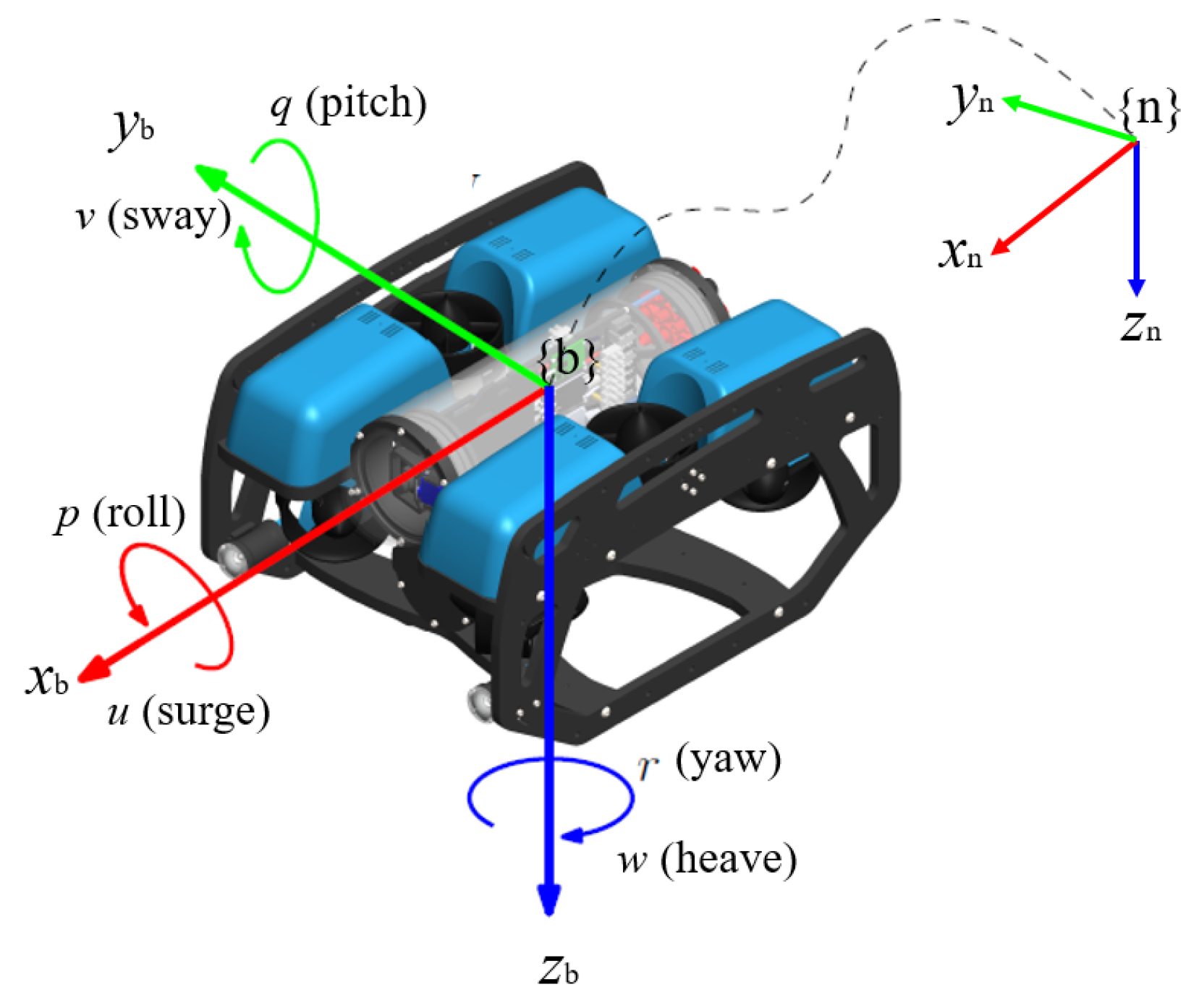
In this study, BlueROV2 (Blue Robotics, Torrance, CA, USA), a commercially available ROV is used. The BlueROV2 depicted in Figure 1 has an open-frame structure with a dry weight of 10 kg and is 457 mm long, 338 mm wide, and 254 mm high. BlueROV2 is ideal for operations in shallow to moderate waters with a standard 100 m depth rating and up to 300 m tether, and comprised of six T200 thrusters together with a rugged frame and quick-swappable batteries. More details about BlueROV2 is given by [32]. The coordinate system used in the ROV analysis is illustrated in Figure 1. To describe the 6-DOF differential nonlinear equation of motion of an underwater vehicle, the equations given by Fossen [33] are applied and can be expressed as

$$M{}_{RB}\dot{v}+C{}_{RB}\left(v\right)v+M{}_A\dot{v_r}+C{}_A\left(v_r\right)v_r+D\left(v_r\right)v_r+g\left(\eta \right)=\tau$$

(1)

in which, $M{}_{RB}$ and $C_{RB}\in {\mathbb{R}}^{6\times 6}$ are the rigid body forces, $M{}_A$, $C{}_A$ and $D\in {\mathbb{R}}^{{}^{6\times 6}}$ represent the hydrodynamic forces; $g\left(\eta \right)$ is the hydrostatic forces. The right-hand term $\tau \in {\mathbb{R}}^{{}^{6\times 1}}$ is the external force term. The hydrodynamics forces is the function of the relative velocity ($v_r$) that between the flow and the vehicle.

For the BlueROV2, the metacentric height provides adequate static stability which guarantee the passive pitch and roll motions and leads to a small roll and pitch angle amplitude. Hence, the nonlinear components of the forces and moments can be considered caused by the viscous effects of the flow, which becomes less important as the pitch angle is small [1]. Therefore, the hydrodynamics behaviour in the surge, sway, heave and yaw are treated as the four principal degrees of freedoms of BlueRov2.

3. Hydrodynamic Model

The fluid dynamics model in this study is based on the Navier-Stokes equations and the continuity equation. Considering an incompressible Newtonian fluid, the momentum and continuity equations can be written as

$$\frac{\partial u_i}{\partial t}+\overline{u_j}\frac{\partial u_i}{\partial x_j}=-\frac{1}{\rho }\frac{\partial p}{\partial x_i}+\nu \frac{\partial u_i}{\partial x_j\partial x_j}$$

(2)

$$\frac{\partial u_j}{\partial x_j}=0(i=1,2,3)$$

(3)

in which x is the Cartesian coordinate, t is the time, u is the velocity, p is the pressure, $\nu$ is the kinematic viscosity and $\rho$ is the fluid density. Subscripts i and j are summation indexes, which represent relevant Cartesian components and equal to 1, 2 and 3 for three-dimension issues in this study. It should be noted that here and throughout this paper, a summation over the range of that index is implied whenever the same index appears twice in any term. In the Reynolds-Averaged Navier-Stokes (RANS) model employed in this study, an ensemble averaging method is applied for the unsteady turbulent flow modelling. The idea is that the unsteadiness in the flow is ensemble-averaged out and regarded as part of the turbulence. The flow variables are represented as the sum of the average and fluctuating term:

$$u_i(x_i,t)=\overline{u_i}\left(x_i\right)+{u_i}^{\prime }(x_i,t)$$

(4)

where the symbols $(-)$ and ${(}^{\prime })$ stand for the average and the fluctuating component, respectively. Repeating a series of measurement with the number of $N_t$ samples, it can be described as

$$\overline{u_i}\left(x_i,t\right)=\frac{1}{N_t}\sum _{n=1}^{N_t}{u}_{ni}\left(x_i,t\right)$$

(5)

in which $N_t$ represents the total number of independent trials, $u_{ni}\left(x_i,t\right)$ is $u(x_i,t)$ captured at the nth series. Adopting it to the incompressible continuity equation and substituting Equation (4) to the corresponding momentum equation, it eventually leads to RANS equation

$$\frac{\partial \overline{u_i}}{\partial t}+\overline{u_j}\frac{\partial \overline{u_i}}{\partial x_j}=\frac{\partial }{\partial x_j}\left[-\frac{1}{\rho }\overline{P}{\delta }_{ij}+\nu \left(\frac{\partial \overline{u_i}}{\partial x_j}+\frac{\partial \overline{u_j}}{\partial x_i}\right)-\overline{{u_i}^{\prime }{u_j}^{\prime }}\right]$$

(6)

There are three stress terms on the right-hand side: $-\frac{1}{\rho }\overline{P}{\delta }_{ij}$ is the mean pressure field; ${\delta }_{ij}$ is the Kronecker delta (${\delta }_{ij}=1$ if $i=j$ and ${\delta }_{ij}=0$ if $i\ne j$) and $\nu \left(\frac{\partial \overline{u_i}}{\partial x_j}+\frac{\partial \overline{u_j}}{\partial x_i}\right)$ represents the viscous stress from the momentum transfer at the molecular level, $\overline{{u_i}^{\prime }{u_j}^{\prime }}$ is the Reynolds stresses arising from the fluctuating velocity field. To close the system, following the Newton’s law of viscosity where the viscous stress is proportional to the velocity gradient, this leads to

$${\tau }_{ij}=\mu s_{ij}=\mu \left(\frac{\partial \overline{u_i}}{\partial x_j}+\frac{\partial \overline{u_j}}{\partial x_i}\right)$$

(7)

in which $\mu =\nu \rho$ is the dynamic viscosity of the flow. In the stress tensor matrix, the diagonal components are the normal stresses, and the off-diagonal components are the shear stresses. Since the turbulent kinetic energy k is the half trace of the Reynolds stress tensor, this gives

$$k=\frac{1}{2}\rho \overline{{u_i}^{\prime }{u_i}^{\prime }}$$

(8)

Since the isotropic stress is defined as $\frac{3}{2}k{\delta }_{ij}$. the deviatoric part of the stress can be found by

$$a_{ij}=\overline{{u_i}^{\prime }{u_j}^{\prime }}-\frac{3}{2}k{\delta }_{ij}$$

(9)

The turbulent-viscosity hypothesis is introduced by Boussinesy [34] which analogy to the stress-strain relation for a Newtonian fluid(see Equation (7)), since the turbulent stresses increase as the mean rate of deformation increase. Based on the turbulent-viscosity hypothesis, the turbulent stress can be derived as

$${\tau }_{ij}=-\overline{{u_i}^{\prime }{u_j}^{\prime }}={\nu }_T\left(\frac{\partial \overline{u_i}}{\partial x_j}+\frac{\partial \overline{u_j}}{\partial x_i}\right)-\frac{3}{2}k{\delta }_{ij}$$

(10)

in which ${\nu }_T={\nu }_T(x_i,t)$ refers as the turbulent or eddy viscosity. This hypothesis introduces the macroscopic representations of the micro-scale fluctuating flow. It offers an access to model the overall effects of small vortexes by correlations and meanwhile, resolve the larger eddies through the numerical simulation. Therefore, the computational time is dramatically reduced compared to the direct numerical simulation (DNS) in which the fluctuating flow and small eddies are directly modelled. By substituting Equation (10) into Equation (6), it gives

$$\frac{\partial \overline{u_i}}{\partial t}+\overline{u_j}\frac{\partial \overline{u_i}}{\partial x_j}=\frac{\partial }{\partial x_j}\left[{\nu }_{e}ff\left(\frac{\partial \overline{u_i}}{\partial x_j}+\frac{\partial \overline{u_j}}{\partial x_i}\right)\right]-\frac{1}{\rho }\frac{\partial }{\partial x_j}\left(\overline{P}+\frac{2}{3}\rho k\right)$$

(11)

$${\nu }_{eff}\left(x_i,t\right)=\nu +{\nu }_T\left(x_i,t\right)$$

(12)

where $\nu$ is the constant molecular viscosity and ${\nu }_T(x_i,t)$ is the spatial-temporal dependent turbulent/eddy viscosity, and together they compose the effective viscosity ${\nu }_{eff}(x_i,t)$.

The Equations (2)–(12) are targeted at solving fixed mesh (Eulerian mesh) issues. However, if a moving structure is involved, as in this study, the computational mesh may need to move to conform to the motion of the rigid body. The alternative is introducing an additional treatment, e.g., treat the structure as an additional phase in the modelling system as in the immersed boundary method (IBM). In this study, the flow distribution in the computational domain and the mesh are updated following the motion of the structure and satisfying the adopted non-slip boundary condition on the structure surface. Meanwhile, the body motion is calculated based on the Newton’s 2nd law in which the force due to the fluid distribution variation on the structure is modelled by the pressure updated by Equation (11) on the rigid body surface. This indicated that the above equations require the accompany of a computational mesh which can cope with both the fixed Eulerian mesh and mesh following the body motion. This leads to the Arbitrary Lagrangian-Eulerian (ALE) form equations, which can be written as

$$\frac{\partial u_{Tj}}{\partial x_j}=0$$

(13)

$$\frac{\partial u_{Tj}}{\partial t}+\left(u_{Tj}-u_{bj}\right)\frac{\partial u_{Tj}}{\partial x_j}=\frac{\partial }{\partial x_j}\left[{\nu }_{e}ff\left(\frac{\partial u_{Tj}}{\partial x_j}+\frac{\partial u_{Tj}}{\partial x_i}\right)\right]-\frac{1}{\rho }\frac{\partial p_T}{\partial x_i}$$

(14)

$${\nu }_{e}ff\left(x_i,t\right)=\nu +{\nu }_T\left(x_i,t\right)$$

(15)

in which, $u_T$ and $p_T$ are the ensemble-averaged flow velocity and pressure, respectively. An additional term, $u_{bj}$, is introduced in the convective term to accommodate the movement of meshes when flow subjecting to the motion of the body. If the nodal velocity is following the fluid velocity, i.e., $u_{bj}=u_{Tj}$, Equation (14) is transformed to the corresponding Lagrangian form; whereas if a static body is involved with fixed mesh, i.e., $u_b=0$, Equation (14) convert to a Eulerian form which is same as Equation (11).

OpenFOAM Solver Validation

In this section, the feasibility and the reliability of the OpenFOAM solver are examined at prior. Flow past a circular cylinder frequently serves as a classic example and benchmark in terms of flow separation and vortex shedding physics [35]. Besides, the flow disturbances caused by the interaction between a circular cylinder and the ROV will be one of the main focuses of ORCA project in following next stage. Therefore, the validation is carried out by using a circular cylinder subjected to the uniform current. In the validation, the drag coefficient from the experimental data for $40<Re<5\times {10}^5$ and Schewe [36] for $Re>{10}^5$, and corresponding numerical results from Stringer et al. [37] are compared to that predicted by the OpenFOAM solver. An appropriate turbulent model is desired in calculating the turbulent viscosity ${\nu }_T\left(x_i,t\right)$ in Equation (15). Hence, two classic turbulent models, i.e., $k-ϵ$ and $k-\omega$ SST turbulent models are employed and evaluated, in which the main issues concerned is the drag/lift coefficient (see Equations (16) and (17)) and vortex shedding frequencies that reflected by the Strouhal number ($St$).

$$C_D=\frac{1}{2}\frac{F_D}{\rho u^{2}A}$$

(16)

$$C_L=\frac{1}{2}\frac{F_L}{\rho u^{2}A}$$

(17)

in which, u is the flow velocity; $\rho$ is the fluid density; $F_D$ and $F_L$ are the drag force and the lift force, respectively; $F_D$ and $F_L$ is the force component in the direction of the flow velocity and the cross-flow direction, respectively and A is the cylinder cross-sectional area.

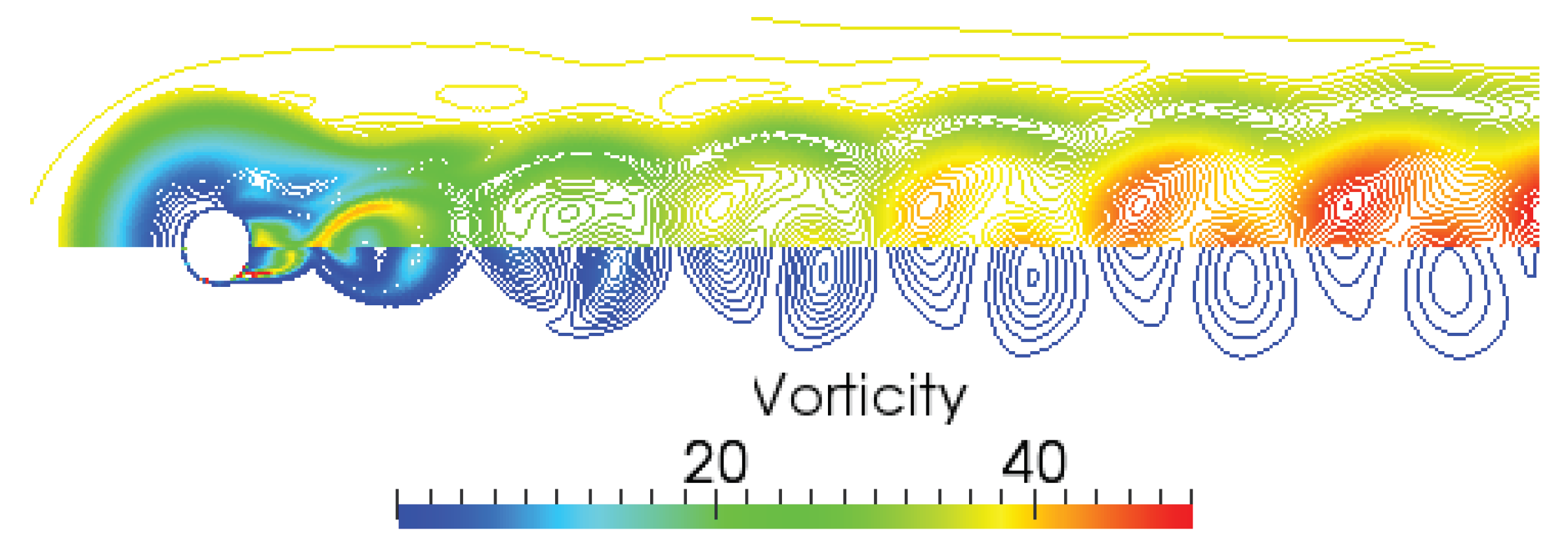
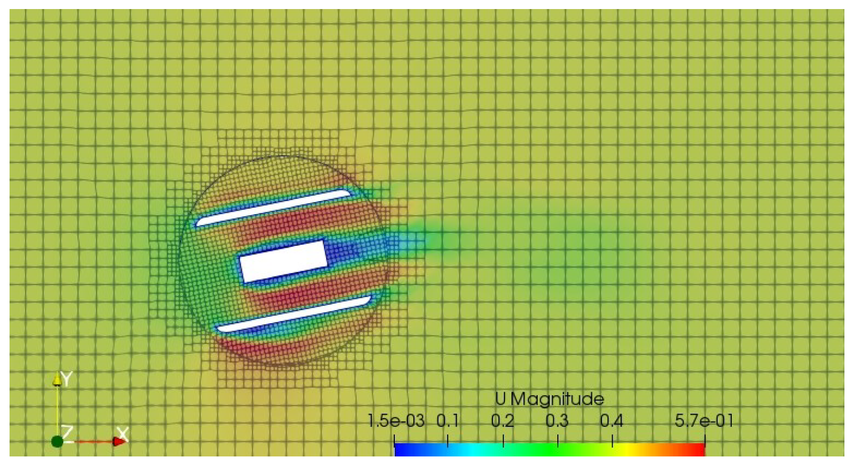
In the flow past a circular cylinder case, it is well understood that after the Reynolds number excess 40, the wake becomes unstable and eventually leads to a set of vortex street shedding alternately on either side of the cylinder at a certain frequency. This also results in the oscillation of the drag force together with the unsymmetrical distribution of the turbulent viscosity ${\nu }_T\left(x_i,t\right)$ and vorticity (see Figure 2). More details about this physics can be seen in [23]. Figure 3 demonstrates the comparisons of $C_D$, from which it is found that $C_D$ predicted by OpenFOAM with $k-\omega$ SST turbulent model generally agrees well with that of the experimental results, and the maximum relative discrepancy (around 13%) is observed at $Re=5\times {10}^5$. Since the drag force is the main concern in this study, the details of lift force comparison is not given here but can be seen in [23]. It should be pointed out that the success of RANS on modelling the turbulent flow largely relying on achieving the desired accuracy of the eddy viscosity. Since the eddy viscosity captured by $k-\omega$ SST model can satisfactorily reflect the macroscopic representation of the fluctuating flow field, one may agree that with the presence of an adverse pressure gradient, the performance of the $k-\omega$ SST is superior to that of $k-ϵ$ model. Based on the fact that RANS solver with $k-\omega$ SST turbulent model can provide predictions fairly close to the experimental data within a large range of $Re$, the same numerical configuration will be employed in the following simulations.

4. Numerical Simulation Configurations

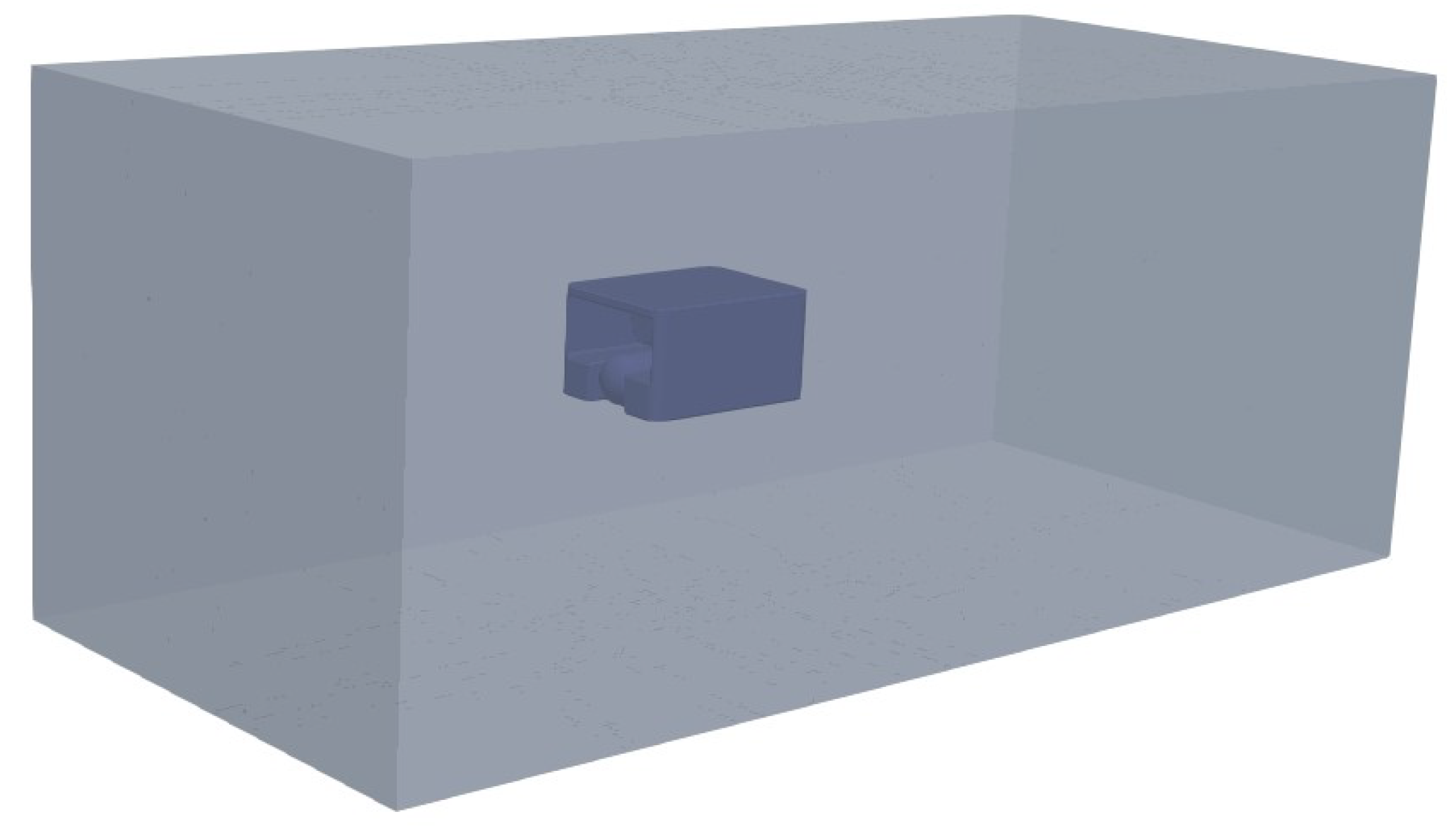
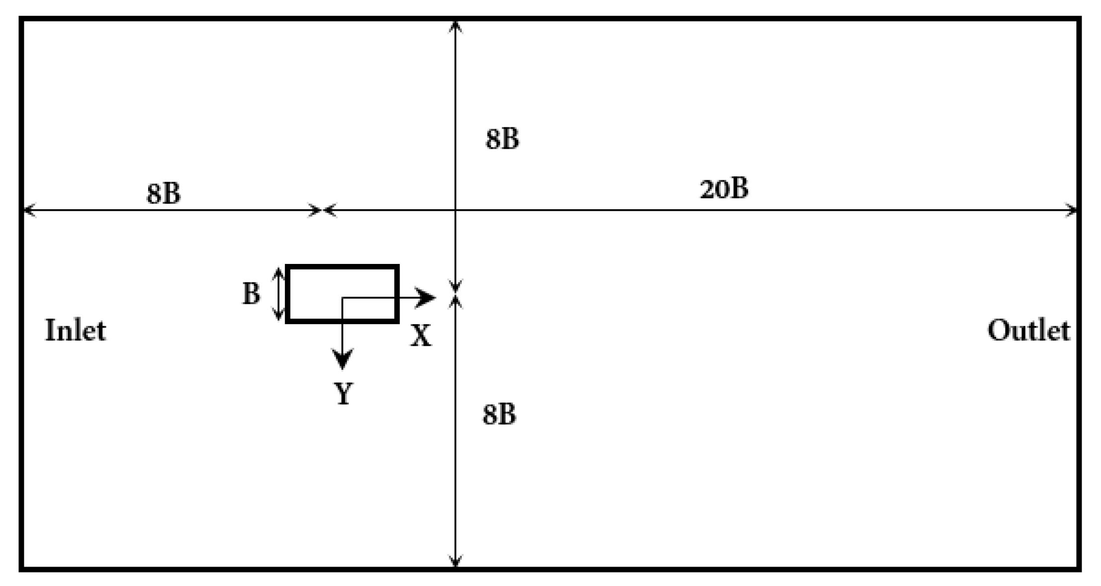
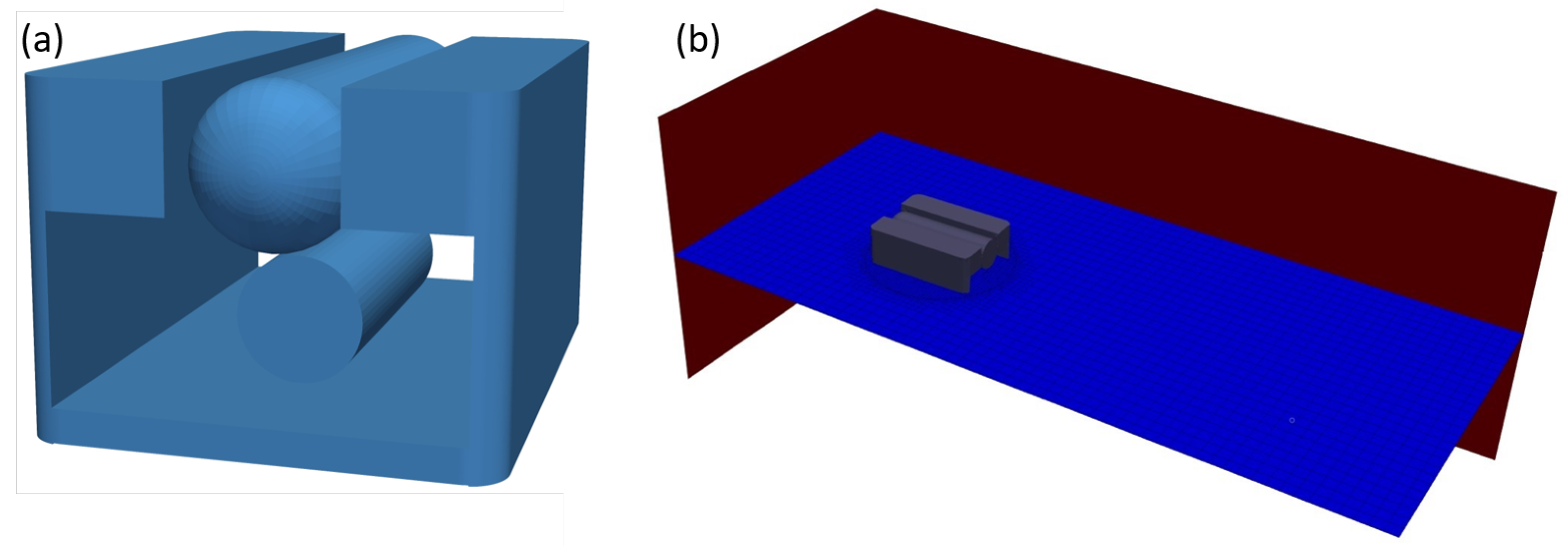
In the numerical simulation, a rectangular computational domain is adopted. The length and the width of the computational domain are $28B$ and $16B$ respectively, where B is the characteristic scale of the ROV. The 3D and 2D views of the computational domains are given in Figure 4 and Figure 5, respectively. The CAD geometry of the vehicle is shown in Figure 6a and the computational mesh is generated by OpenFOAM internal utility snappyHexMesh (see Figure 6b). A series of numerical simulations target on the hydrodynamics performances of the four principal motions (surge, sway, heave and yaw) are conducted with the boundary conditions including: (1) a Neumann zero-gradient velocity boundary condition is implemented at the outlet boundary; (2) a slip boundary condition is applied at the top, bottom, front and back boundaries and (3) a non-slip condition is used on the body surface.

The investigations are performed at the Reynolds number ranging from $6.76\times {10}^4$ to $3.38\times {10}^5$ which corresponds to an incoming current velocity between 0.2 m/s to 1.0 m/s, with $\rho =$ 1025 kg/m${}^3$, $\nu =1\times {10}^{-6}$ m${}^2$/s and the characteristic length is 0.338 m. One may agree that all CFD work is highly dependent on the mesh resolution. Therefore, for each of the four degree of freedoms, the convergence test against mesh resolution is performed to identify the suitable mesh configuration with a minimal computational cost. Wall treatment is always one of the biggest challenges raised in the turbulent flow simulation, which can be classified into two categories: the low-Reynolds-number ($LR$) models and high-Reynolds-number ($HR$) models. The low-Reynolds-number ($LR$) approach accompanied by a wall functions is targeting at the sublayer where exists a local low turbulent Reynolds number. One alternative to wall functions is to adopt a fine-grid configuration that allows the application of a laminar flow boundary condition. To reach the viscous sublayer, the normalized distance ($y^{{}_{+}}$) from the first mesh cell centre to body surface is supposed to be around 1, where $y^{{}_{+}}=u_{*}y{}_w/{\nu }_{eff}$. In the numerical practice, the desired $y^{{}_{+}}$ is usually obtained through consistent trials. However, the $HR$ model can cope with a much larger $y^{{}_{+}}$ (around 30) which integrates with a log law to estimate the gradient approaching the body wall. It should be noted that the first computational mesh should be placed either in the log-layer or the viscous sublayer but not in-between [38], since none of the categories can deal with the buffer layer where both viscous and Reynolds stresses are significant. Within certain mesh configuration, the time step size $\Delta t$ is automatically determined by using the fixed Courant number $C_0$ ($C_0=\left(u\Delta x\right)/\Delta t$, where $\Delta x$ is the mesh size).

5. Experiment Setup

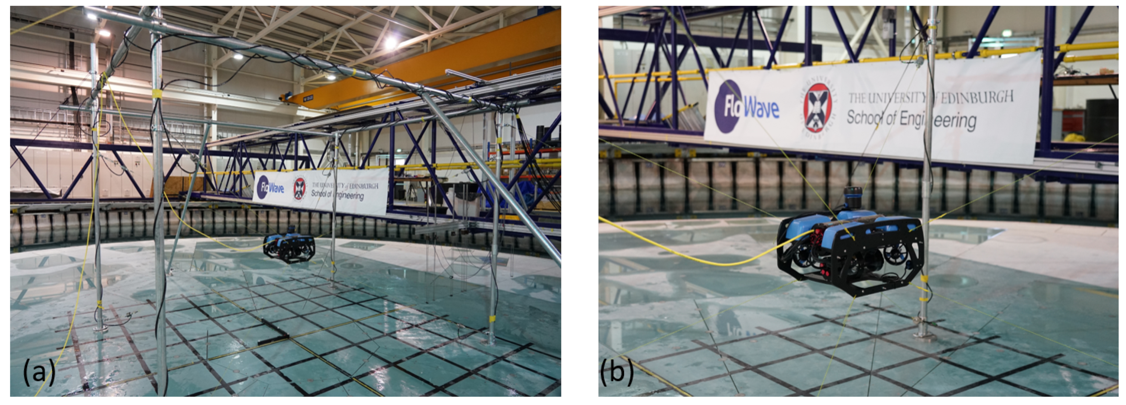
In this study, a new test technique was designed to quantify the hydrodynamic forces on a ROV in the FloWave facility. FloWave is a 25 m diameter circular tank with a total water depth of 2 m. The floor of the tank is buoyant and can be raised out of the water for model installation and the water currents can be generated from any direction of the tank (see Figure 7). More details of the FloWave current generation are provided in [30]. During the test, the ROV was connected to eight tethers to the frame at the height of 1 m from the floor (see Figure 7a). The configurations of the frame and tethers are given by Gabl et al. [31]. The measurement instrumentation used were: (1) motion capturing system (MoCAP) to record the motion and rotation of the different structures, (2) load cells to measure the forces along the eight tethers. The MoCAP worked together with four underwater cameras provided by Qualisys. Knowing the position of the ROV, the mounting points (connection of the tether to the ROV) can be calculated as the virtual points. This allowed the direction of the force vector can be accurately determined and three-dimensional force components to be resolved. The working conditions tested in the model test can be seen in

Table 1. Experimental test working conditions.

	Surge	Sway
Flow velocity [m/s]	[0.2–1.0]	[0.2–0.6]
Direction [degree]	180/$-180$	$-90$/90
Capture time [s]	512	512

. For the surge drag measurement, the velocities examined was ranging from 0.2 m/s to 1.0 m/s with a increment of 0.2 m/s, and in both the forward and backwards surge directions. For the sway drag, a smaller velocity range which up to 0.6m/s was tested, and also in the forward and backwards sway directions.

6. Results Discussion

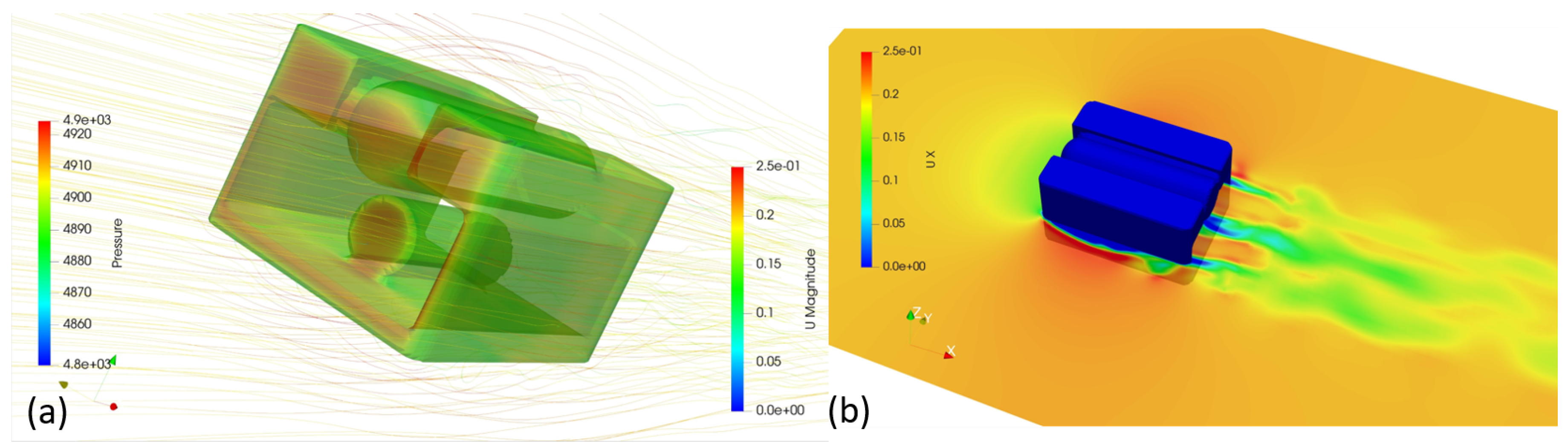
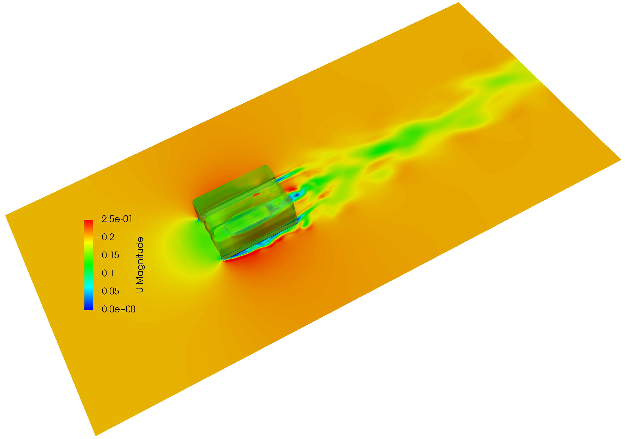
The physics and quantified hydrodynamic forces on a ROV from the numerical simulation and experimental test are analysed and compared in this section. Figure 8a) reveals the instantaneous pressure distribution on the vehicle and the streamlines around the vehicle. Higher pressure is observed at the front of ROV while the wake at the rear creates a low-pressure region. Correspondingly, a low velocity area at the front of the ROV is captured which can be seen from Figure 8b).

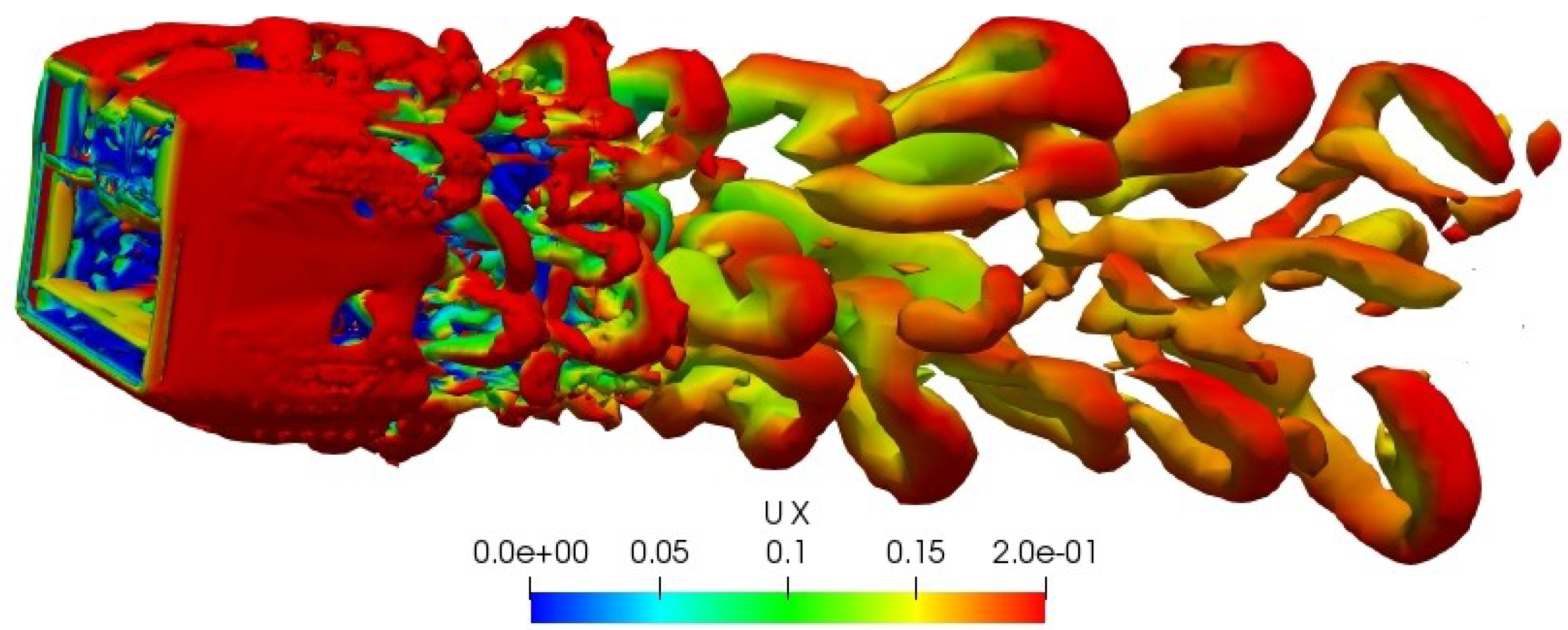
The flow separations and flow interactions between different parts of the vehicle are exhibited. There are three individual shedding first generated by the left, right frame and centre structure of the vehicle, respectively. Strong interactions among them are observed with the development of the flow which eventually results in a single shedding moving towards the outlet. The development of the turbulent vortices is captured which is triggered by the flow separation at the wake of the vehicle (see Figure 9 and Figure 10). The isosurfaces in Figure 9 are visualized vortices using Q criterion and coloured with stream-wise velocities. The separated flow and the corresponding shedding significantly alters the flow pattern at the wake of the ROV which leads to the non-linear and fluctuating drag forces acting on the ROV.

The instantaneous velocity field of the vehicle under the yaw motion is demonstrated in Figure 11. Three sets of individual vortex shedding are formed at the rear of the vehicle, but due to the inlet flow direction is not aligned with the vehicle movement direction in the rotational motion, the interactions between the three sets of the shedding are not as strong as that in the translational motion.

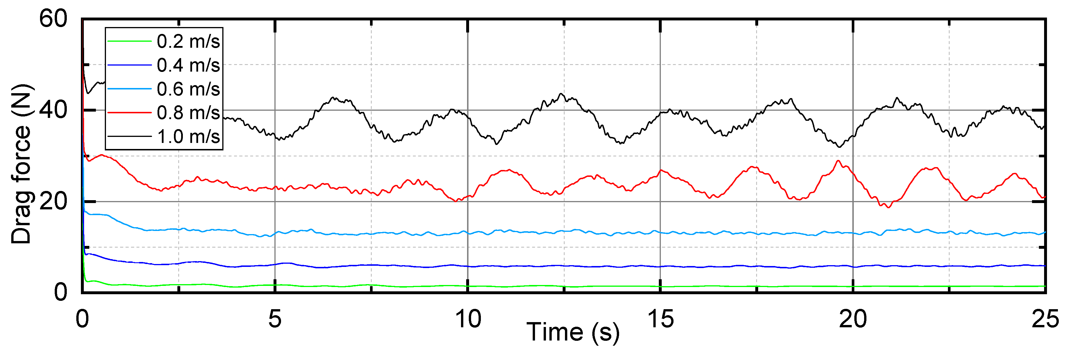
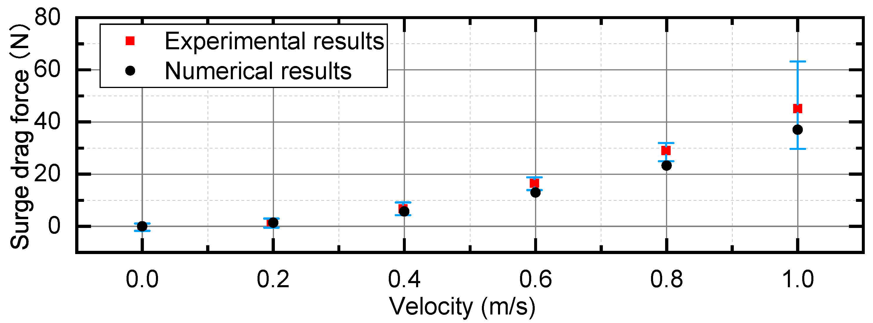
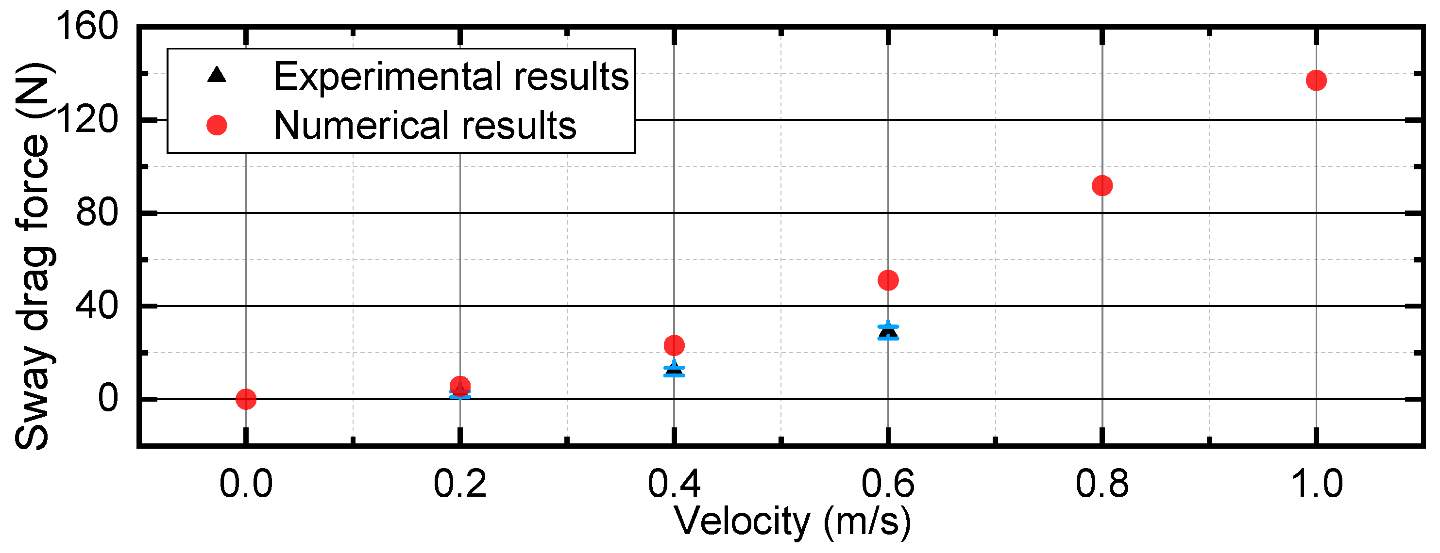
Figure 12 demonstrates the time series of surge drag force exerting on the ROV under the flow velocities ranging from 0.2 m/s to 1.0 m/s. The surge and sway drag forces measured by the test are compared to the numerical results in Figure 13 and Figure 14, respectively. For the surge drag, it can be observed that a good agreement is achieved throughout the velocity range. However, the discrepancy between the numerical and experimental result is increasing with the increase of the velocity acting on the ROV. Similarly, the same trend is exhibited in the sway drag comparison, with the maximum discrepancy appears at the largest velocity tested (0.6 m/s). The major sources of errors in the numerical simulations include the neglect of the geometry details, such as attached propellers and tether. Other error sources may the differences between the turbulent flow generated by the turbulent model and the reality in the FloWave.

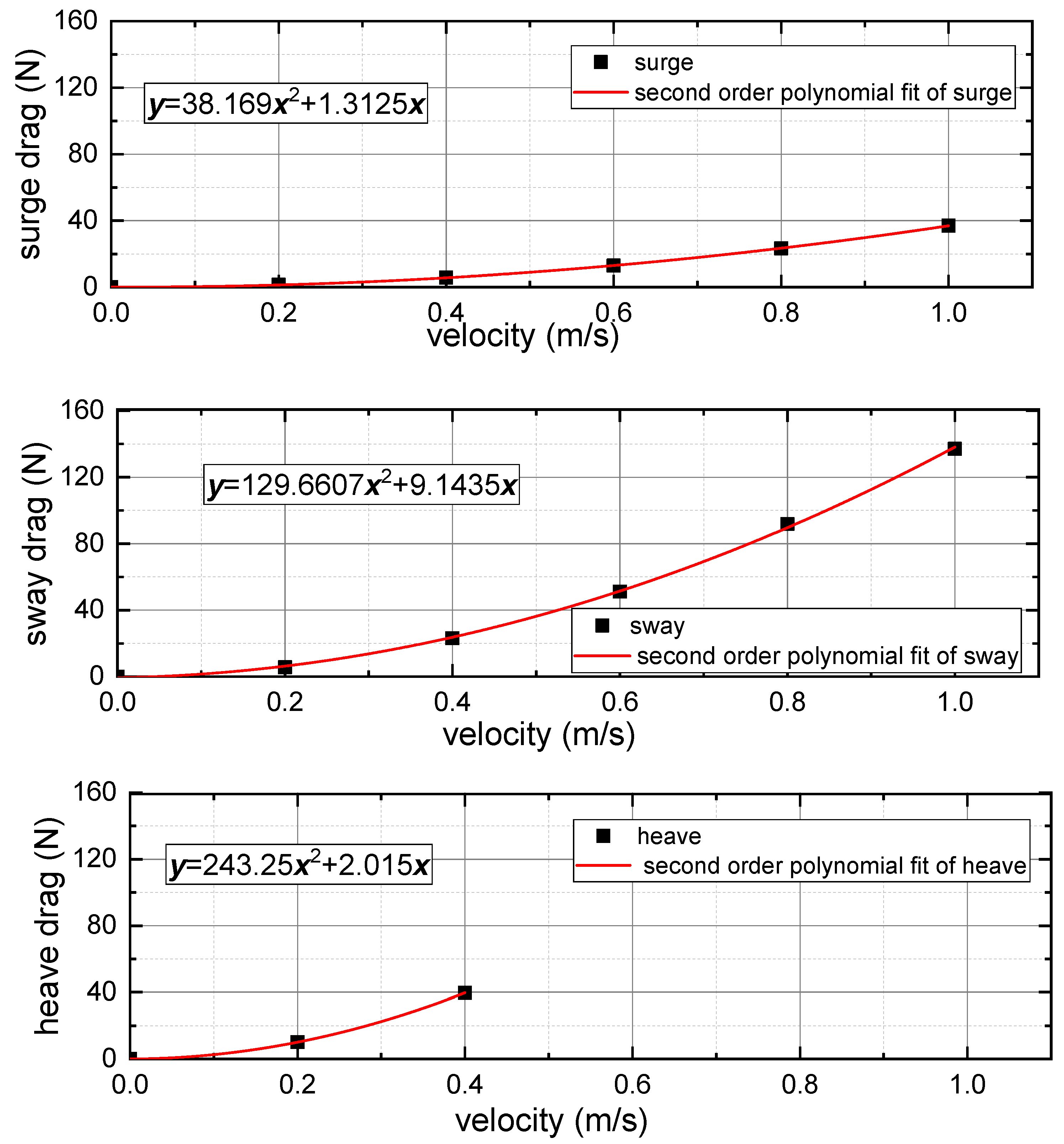
The damping coefficients for each direction are obtained by using a second-order polynomial fit (see Figure 15), and the resulting drag coefficients of the vehicle in its four principal DOFs are given in

Table 2. Table to test captions and labels.

Damping Coefficient	Surge		Sway		Heave		Yaw
	KL	KQ	KL	KQ	KL	KQ	KL	KQ
Values	1.3125	38.169	9.1435	129.6607	2.015	243.25	0	4.86

. As exhibited in Figure 15, the largest drag is observed in the heave motion due to its largest frontal area in the X-Y plane. Meanwhile, the drag force in the sway motion is slightly larger than that in the surge motion since the frontal area in the Y-Z plane is smaller than that of X-Z plane.

7. Conclusions

In this study, a numerical model within the frame of OpenFOAM is proposed, which is capable of simulating multi DOFs motions and turbulent flow problems. We investigated the hydrodynamic behaviour of the BlueROV2 which is complex with an open frame structure. The accuracy and reliability of the numerical model are validated by the experiential test, in which a new test method targeted at the force and moment measurement of the vehicle is designed. With the hydrodynamic coefficients found by the numerical simulation, a more robust and stability control system can be designed in the dynamic positioning of ROV when facing the combined effect of current and turbulence. Besides, the hydrodynamic disturbances acting on the vehicle can be treated as external forces within the nonlinear ROV dynamic and propulsion model to improve its disturbance rejection performance. The good agreement with the experimental result builds the confidence of applying the proposed methodologies to more complex working scenarios. For instance, the marine renewable energy facilities are typically deployed in the shallow water environments where is characterised by strong hydrodynamic forces involving both wave and current. In future work, the disturbances triggered by the presence of the flow surface should be tracked where a two-phase solver is required. Furthermore, the modelling of the nonlinear disturbances considering the direction between the wave and current is desired too.