
Optimizing the Production-Living-Ecological Space for Reducing the Ecosystem Services Deficit

1
School of Earth Science and Resources, Chang’an University, Xi’an 710054, China
2
School of Land Engineering, Chang’an University, Xi’an 710054, China
3
The Key Laboratory of Shaanxi Land Consolidation Project, Chang’an University, Xi’an 710054, China
*
Author to whom correspondence should be addressed.
Land 2021, 10(10), 1001; https://0-doi-org.brum.beds.ac.uk/10.3390/land10101001
Submission received: 18 August 2021
/
Revised: 16 September 2021
/
Accepted: 17 September 2021
/
Published: 23 September 2021
(This article belongs to the Special Issue Land Use Conflict Detection and Multi-Objective Optimization Based on the Productivity, Sustainability, and Livability Perspective)
Abstract
:With rapid urbanization and industrialization, China’s metropolises have undergone a huge shift in land use, which has had a profound impact on the ecological environment. Accordingly, the contradictions between regional production, living, and ecological spaces have intensified. The study of the optimization of production-living-ecological space (PLES) is crucial for the sustainable use of land resources and regional socio-economic development. However, research on the optimization of land patterns based on PLES is still being explored, and a unified technical framework for integrated optimization has yet to be developed. Ecosystem services (ES), as a bridge between people and nature, provide a vehicle for the interlinking of elements of the human-land system coupling. The integration of ES supply and demand into ecosystem assessments can enhance the policy relevance and practical application of the ES concept in land management and is also conducive to achieving ecological security and safeguarding human well-being. In this study, an integrated framework comprising four core steps was developed to optimize the PLES in such a way that all ecosystem services are in surplus as far as possible. It was also applied to a case study in the middle and lower reaches of the Yellow River Basin. A regression analysis between ES and PLES was used to derive equilibrium thresholds for the supply and demand of ES. The ternary phase diagram method was used to determine the direction and magnitude of the optimization of the PLES, and finally, the corresponding optimization recommendations were made at different scales.
1. Introduction
Since the 20th century, along with the acceleration of global urbanization and industrialization, the continued large-scale exploitation of land resources has been accompanied by environmental problems, such as the crowding of ecological space by urban construction land, atmospheric pollution, water pollution, and ecological imbalance [1,2,3]. Since the reform and opening up of China in 1978, urbanization and industrialization have advanced rapidly. At the end of 2018, 59.6% of China’s land was urbanized, and China has entered a period of steady urbanization [4,5]. In this context, structural imbalances in land use have come to the fore, the contradiction between production-living-ecological space (PLES) has become increasingly prominent, and land use is facing enormous pressure and challenges [6,7]. Therefore, to promote regional sustainable development and the effective and efficient application of land space, it is necessary to reasonably allocate limited spatial resources [8,9,10]. Integrating the spatial functions and land use structure under the PLES linkage and promoting the coordinated development of the quantitative structure and spatial layout of the PLES has become an urgent issue to be addressed [11,12].
Ecosystem services (ES), as a bridge between natural ecosystems and human well-being, are the various benefits that humans derive directly or indirectly from ecosystems [13,14]. Ecosystem services depend on the interactions and feedback between ecological and socio-economic factors [15,16]. Humans manage ecosystem processes by modifying ecosystem components and structures to provide ES that better meet their needs [17,18]. A common way of doing this is improving human well-being by changing land use/cover, e.g., converting other lands to cropland can improve food production service. The conversion of arable land and grassland into forest land can improve water yield services, soil conservation services, and carbon sequestration services, etc. [19]. The gradual deepening and formation of the concept of ES provides a vehicle for interlinking the elements of human-land system coupling [20,21]. As a result, the concept of ES is now becoming increasingly important at the land management level [22,23].
With the deepening of ES research, a large number of researchers have begun to focus on both the ES supply (i.e., the capacity of ecosystems to provide ecosystem goods and services to humans) and the ES demand (i.e., the sum of ecosystem goods and services used or consumed by humans) [24,25]. The gradual intensification of global climate change, environmental pollution, and human-land conflicts have led to changes in ecosystem structure and function, affecting the supply capacity of ES [26,27]. Meanwhile, the increasing level of urbanization and industrialization has led to the emergence of a large number of ES demand aggregation centers [28,29], further exacerbating the mismatch between ES supply and demand. Incorporating ES supply and demand into ecosystem assessments can improve the policy relevance and practical application of the ES concept in land management. It is also conducive to achieving ecological security and safeguarding human well-being [30,31].
There is often a desire to maximize the ES supply through land management to reduce mismatches and shortages, but a major challenge is to integrate analysis to avoid unnecessary trade-offs in ES [32,33]. In this context, exploring spatial mismatches between ES supply and demand associated with urbanization-related land use is crucial for the proper integration of ES into land management strategies [34]. Many studies have considered both ES supply and demand and have identified potential mismatches between ES supply and demand at multiple scales [35]. The challenge is that most ES assessments have not yet been effective in influencing land management decisions and, in particular, lack holistic considerations [36,37]. The PLES covers the spatial range of activities of human social life and is the basic vehicle for human economic and social development [38]. The three are both independent and interrelated, with symbiotic integration and constraining effects, and the collaboration of PLES functions can produce a synergistic effect in which the overall function is greater than the sum of the partial functions [39]. The PLES optimization belongs to the problem of optimizing the allocation of national land resources. Based on land characteristics and land-use system principles, the structure and direction of land resource use are arranged, designed, combined, and laid out at a hierarchical level on a spatial and temporal scale to improve the efficiency and effectiveness of land use, maintain the relative balance of land ecosystems, and realize the sustainable use of land resources [40]. The main theoretical support for current PLES optimization comes from the theory of regional resource and environmental carrying capacity and the theory of coupling urbanization and ecological environment [41,42]. This study focuses on the consideration from the perspective of ecosystem services, and it is a new attempt to apply the assessment of ecosystem service supply and demand to the optimization of PLES.
The Yellow River Basin, an important ecological barrier, straddles three regions in the east, central, and west of China and is an ecological corridor connecting the Qinghai-Tibet Plateau, the Loess Plateau, and the North China Plain. Although breakthroughs in ecological construction and environmental management have been made in the Yellow River Basin in recent years, the fragile ecological environment, water scarcity, and water environment problems are outstanding. especially in the middle and lower reaches of the Yellow River, which have undergone rapid urbanization over the past decades, leading to huge changes in the spatial pattern of land use, accompanied by huge landscape changes and related degradation of ES. Therefore, this study takes the Yellow River basin as an example to explore the spatial patterns of ES supply and demand and the response to PLES changes and to identify optimization areas through response thresholds to provide optimization strategies for land use at multiple scales.
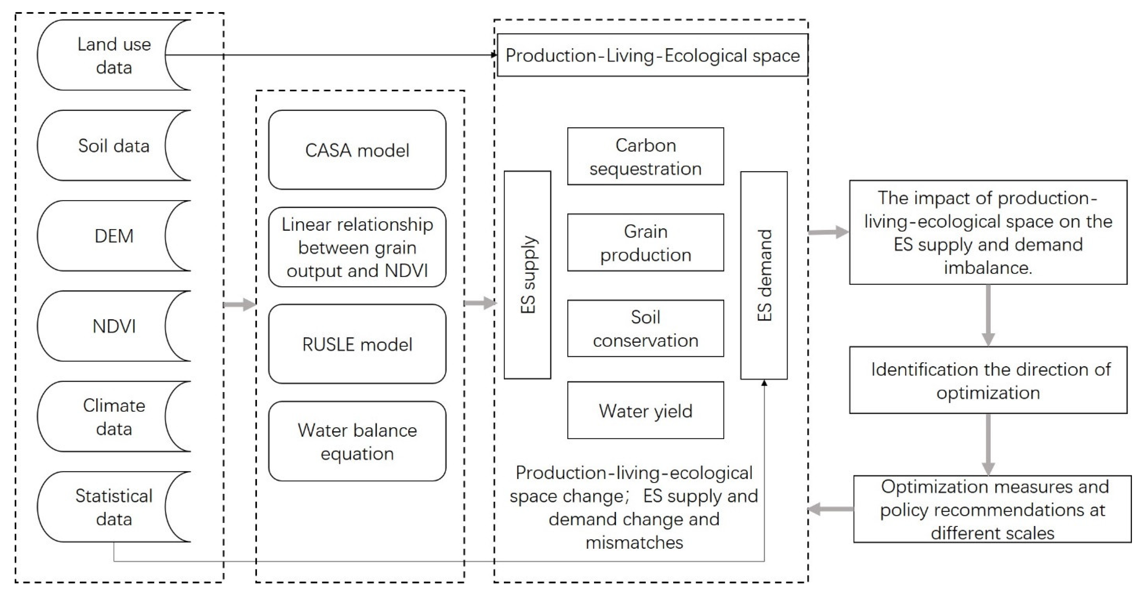
Land use optimization is a complex concept [43]. This study has envisaged an ideal area where optimal PLES management reduces ES deficits and mismatches, to which the land use pattern of the remaining areas should be as close as possible. The basic optimization four steps included: (1) classifying production-living-ecological spaces based on land use types; (2) choosing key ES, quantifying ES supply and demand, and identifying spatial mismatches; (3) identifying the impact of PLES on the spatial mismatch of ES and thresholds; (4) determining the direction of optimization and proposing optimization solutions for different spatial scales.
The selection of key ES was based on the following principles: (1) spatially quantifiable mapping; (2) consistent with the focus of regional governments and residents; (3) better representation of the coupling mechanisms between different ES; (4) availability of measurement data. In this study, the carbon sequestration service, water yield service, soil conservation service, and grain production service were selected as indicators for measuring the ES supply and demand in the Yellow River Basin to minimize the deficit and mismatch of these four ES and carry out corresponding PLES optimization.
2. Materials and Methods
2.1. Study Area
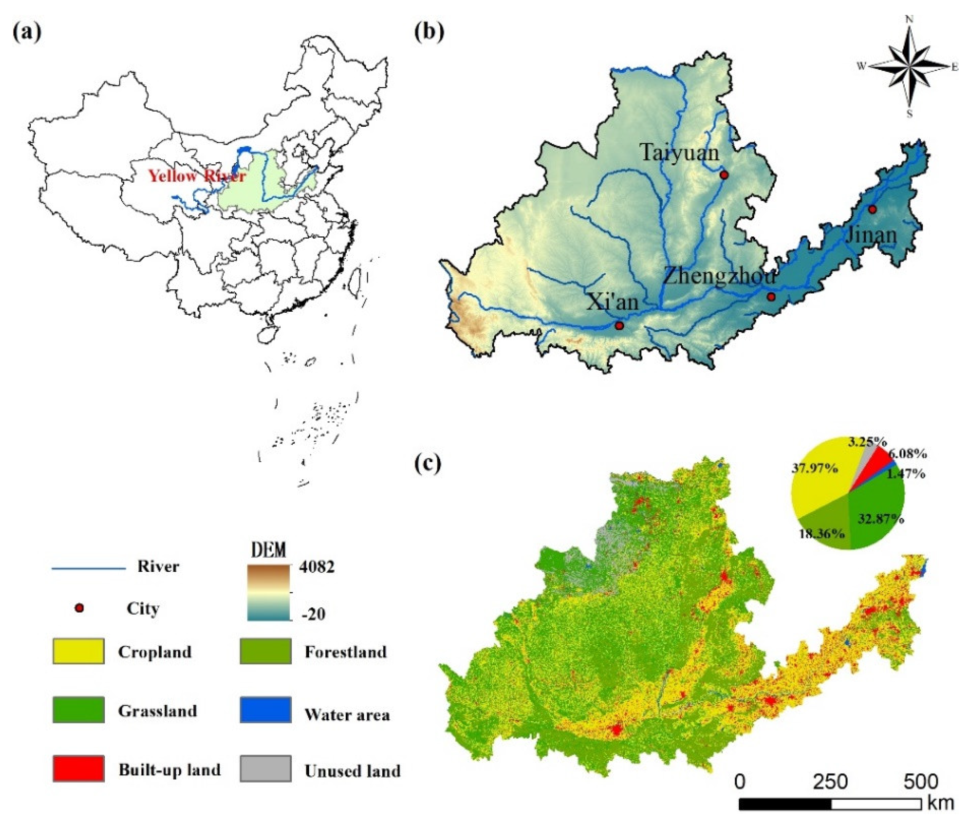
The study area was in the middle and lower reaches of the Yellow River basin (103°36′–119°55′ E, 41°03′–32°46′ N), at an altitude of about 0–4082 m. The area was located in the central-eastern part of China (Figure 1). The main provinces involved included Inner Mongolia Autonomous Region, Henan Province, Shaanxi Province, Shanxi Province, Qinghai Province, and Gansu Province. The middle and lower reaches of the Yellow River Basin are dominated by plains and hills. The region has a temperate continental climate and a temperate monsoon climate. The middle and lower reaches of the Yellow River Basin have abundant light, high temperature, abundant precipitation, are suitable for crop growth, and are the main production areas for agricultural products. The Yellow River Basin is an important economic zone and an important base for energy, chemicals, raw materials, and basic industries in China.
2.2. Data Sources
In this study, we used data from five different sources. (1) Meteorological elements and daily precipitation for 2000, 2010, and 2018, supplied by the China Meteorological Data Sharing Network (http://data.cma.cn/ (accessed on 1 July 2021)), were batch interpolated using the professional meteorological interpolation software ANUSPLIN. (2) Monthly NDVI data for 2000, 2010, and 2018 at a spatial resolution of 1 km × 1 km, supplied by the Geospatial Data Cloud (http://www.gscloud.cn/ (accessed on 1 July 2021)), and annual NDVI data were obtained using the maximum synthesis method. (3) Population data for 2000, 2010, and 2018 at a spatial resolution of 1 km × 1 km was supplied by WorldPop (https://www.worldpop.org/ (accessed on 1 July 2021)). (4) Land use data for 2000, 2010, and 2018 at a spatial resolution of 1 km × 1 km was supplied by the Resource and Environmental Science and Data Centre (http://www.resdc.cn/ (accessed on 1 July 2021)). (5) Grain production, energy consumption, and water consumption by the municipality for 2000, 2010, and 2018 was obtained from the statistical yearbooks and water resources bulletins of each province.
2.3. Framework for Optimizing Production-Living-Ecological Space
Based on previous approaches and frameworks for land use optimization [23,44], this study identified ideal land-use patterns and optimized PLES at different scales by quantifying the mismatch between the supply and demand of ES associated with PLES. This was achieved through the following four core steps (Figure 2): In the first step, the composition, configuration, and spatial transition of PLES were analyzed based on land use data in the Yellow River Basin during 2000, 2010, and 2018. This step aims to examine the spatial changes in PLES in the Yellow River Basin during 2000, 2010, and 2018, and establish a basis for subsequent research. In the second step, those ES suitable for the Yellow River Basin were selected based on the basic principles for the selection of ES proposed above to assess the ES supply and demand. Mismatches and shortages between ES supply and demand were also identified. In the third step, based on the correlation between the ratio of production/living/ecological space and the supply and demand of ES, the thresholds were identified when ES supply and demand were imbalanced. This step aims to analyze the links that exist between the two, the most central part of which is the identification of thresholds. In the fourth step, the thresholds identified in the previous step were used to identify optimization areas using ternary phase diagrams, which were then optimized for PLES at different scales.
Step 1: The classification of production-living-ecological space based on land use types.
Production space is mainly the area that provides various products or services for people. Living space refers to the area that provides the function of carrying and guaranteeing human habitation and provides the function of residence, consumption, leisure, and recreation in the country. Ecological space refers to the area that can provide an ecological barrier and has the function of regulating the atmosphere, concealing water, and maintaining soil and water [11,12]. In this study, a classification system for PLES in the Yellow River Basin was constructed based on geographical features and previous research results [45] (Table 1).
Step 2: Quantify ES supply and demand and identify spatial mismatches.
(1) Quantifying ES supply and demand
Water yield service are the ability of an ecosystem to intercept or store water resources from rainfall while mitigating ground runoff [46]. The Yellow River Basin is an important water source in northwest China and assessing the water yield service is of great practical importance for the rational use and conservation of water resources. The water balance model was used to calculate the supply of water yield service [47]. The amount of water consumed per capita in each city in the Yellow River Basin was obtained from data on industrial, agricultural, and domestic water consumption and the resident population of each city and combined with data on population density to obtain the demand for water yield services. The formulas are as follows.
where represents the annual average yield at pixel x (m3); is the average annual precipitation on pixel x (mm); is the actual annual evapotranspiration at pixel x (mm); is based on the Penman-Monteith formula [48]. is water demand, which in this case equates to water consumption (m3); is water consumption per capita (m3/ person), which includes water consumption for agricultural, industrial, domestic, and ecological purposes; is the local resident population density (person/km2).
Grain production service, as one of the basic ecological services, plays a vital role in human survival and development [49]. There is a significant linear relationship between crop and livestock production based on the NDVI. The total production of grain was allocated according to the ratio of raster NDVI values to total arable land NDVI values, which in turn characterized the grain production capacity of each raster. Grain demand was estimated by multiplying the per capita grain demand by the population density [17]. The formulas are as follows:
where is the total production of grain for grid x (t/km2); is the production of grain products for each province (t); is the normalized difference vegetation index for grid x; is the sum of NDVI of cropland for each province; is the grain demand (t/km2); is the annual per capita grain consumption (t/person); is the resident population density (person/km2).
Carbon sequestration services are important regulatory services in ecosystems. The CASA model is a common model for calculating NPP due to its high calculation accuracy and easy-to-access data and parameters [50]. The carbon sequestration demand was calculated from the product of population density, per capita energy consumption, and energy carbon conversion rate, where energy consumption was obtained from the statistical yearbooks of the Yellow River Basin provinces. The formulas are as follows:
where NPP is the net primary productivity of the pixel x at time t (gC/m2·a); APAR is the Absorbed Photosynthetic Active Radiation (MJ/m2·a), which is estimated from the ratio of total solar radiation (SOL) to absorbed photosynthetically active radiation (FPAR); is the efficiency of conversion of photosynthetically active radiation to organic carbon (gC/MJ2), which is estimated by maximum light energy utilization (0.389 gC/MJ2), temperature stress (Tε), and water stress (Wε). represents carbon sequestration demand (t/km2); is the annual per capita carbon consumption (t/person); is the resident population density (person/km2).
Soil conservation service reduces soil erosion and restores soil fertility, which is critical to agricultural production [51]. This study quantified the soil conservation service supply based on the classical revised universal soil loss equation (RUSLE). The ecosystem service demand is the number of ecological goods that humans expect to be able to obtain from an ecosystem. Since actual soil erosion causes unwanted human losses and humans expect to manage these actual amounts of soil erosion, the actual amount of soil erosion is defined as the soil conservation service demand. The formulas are as follows:
where is soil conservation; is actual soil erosion; is the precipitation erosion factor; is the soil erosion factor; is slope length factor; is soil conservation factor; is vegetation cover factor [52].
(2) ES supply and demand mismatches and shortfalls
The supply and demand of ES are significantly spatially heterogeneous and are reflected in spatial mismatches. The state of ES supply and demand can be characterized by the ecological supply-demand ratio (ESDR), which can be used to reveal the nature of surpluses or deficits [35,53].
where and refer to the ES supply and demand, respectively; is the maximum value of the ES supply; is the maximum value of the ES demand. > 0 indicates a surplus, = 0 indicates a balanced ES supply and demand, and < 0 indicates a deficit.
Step 3: The impact of production-life-ecological space on the ES supply and demand imbalance.
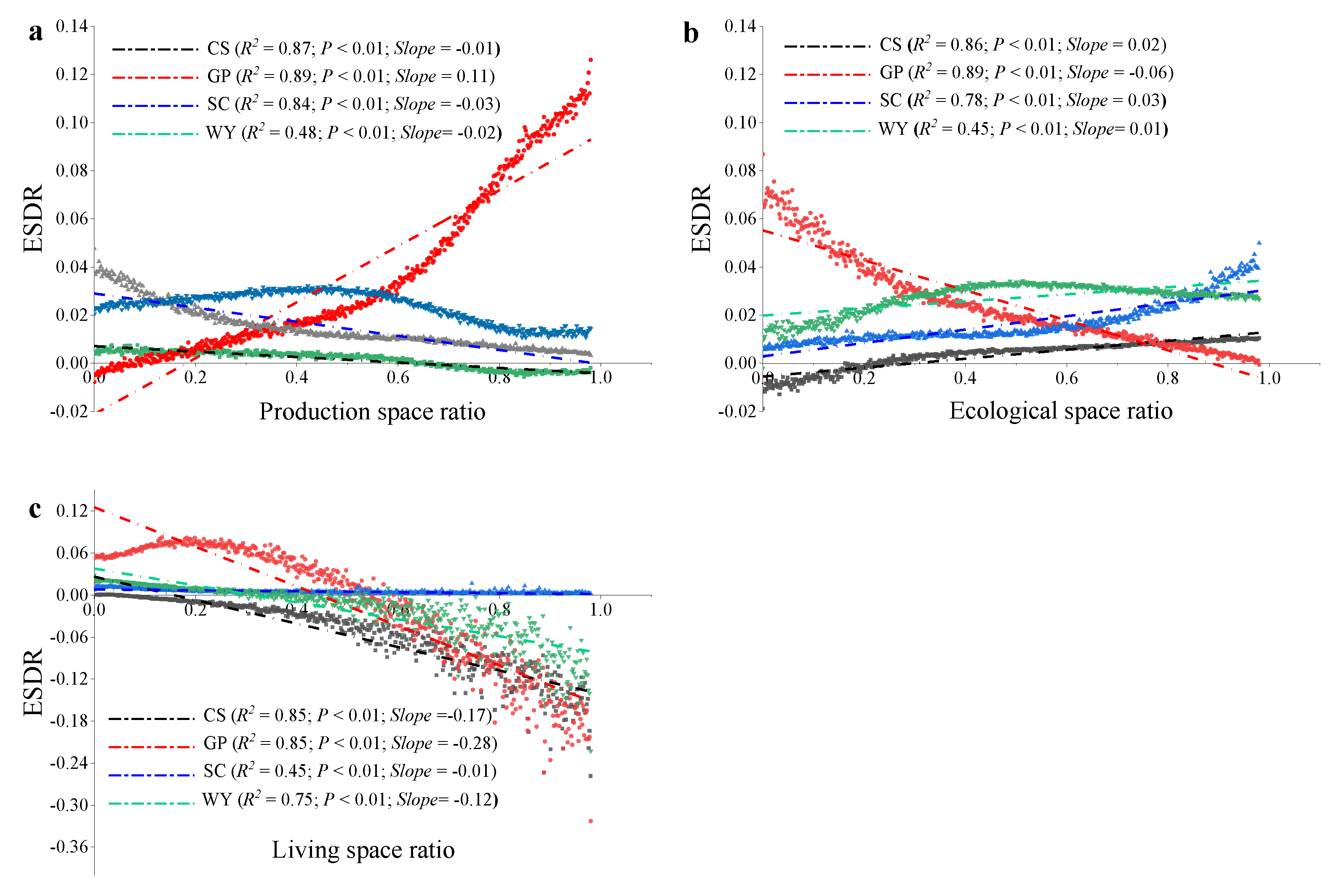
The ESDRs for the four major ES in 2000, 2008, and 2018 were calculated by the above method, while the production space ratio/living space ratio/ecological space ratio at the 1 km grid scale was calculated based on 30 m land use data. The data were statistically graded for the years 2000, 2010, and 2018, and then least squares regression analysis was conducted via SPSS to plot the trend line between ESDR and production space ratio/living space ratio/ecological space ratio to indicate negative or positive effects and significance levels. Spatial land management thresholds (i.e., the ratio of production-living-ecological land when there is a deficit in the ES) were then calculated based on the results of the regression analysis.
Step 4: Identification of the direction of optimization and policy recommendations.
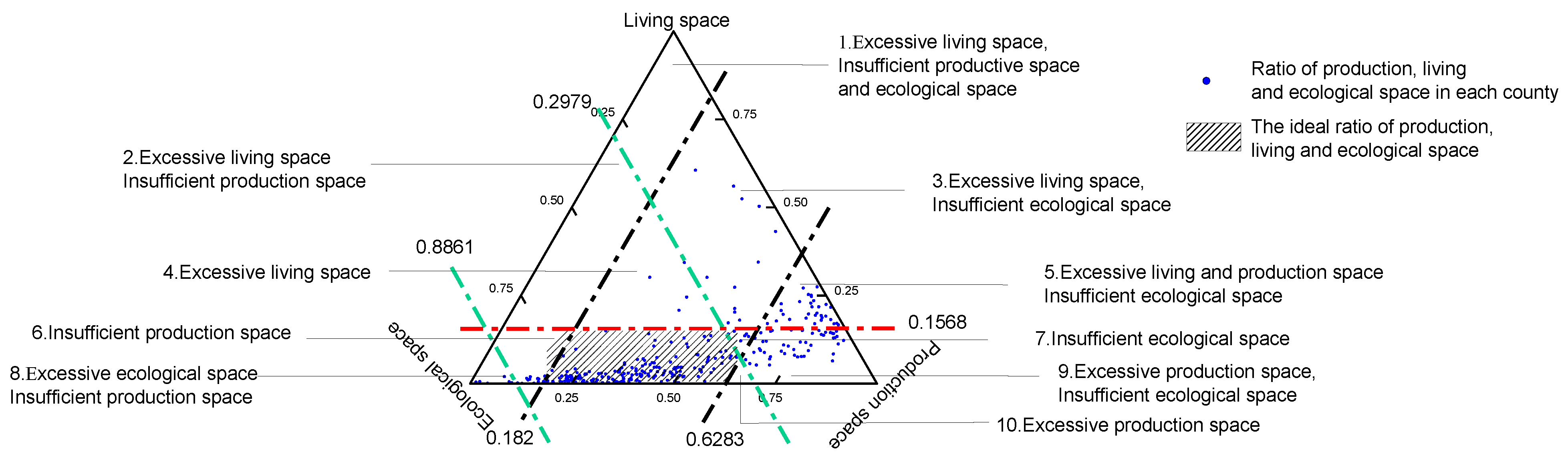
A ternary diagram is a type of center of gravity diagram that has three variables but requires the sum of the three to be constant. In an equilateral triangular coordinate system, the position of a point in the diagram represents the proportional relationship between the three variables. In this study, the same ternary was used to visually express the ratio of production-living-ecological space, which was used to identify the optimization area with the main optimization direction, where the ratio occupied by this type of land at the endpoint is 100%. The regions are divided according to the thresholds determined above. The projection of units of different scales is performed, and when the projection falls in the ideal region, it means that the unit does not need to be optimized, and when it falls in other regions, the direction and quantity relationship of optimization can be determined based on the direction and distance from the ideal region.
3. Results
3.1. Structure and Transition of PLE Land Use
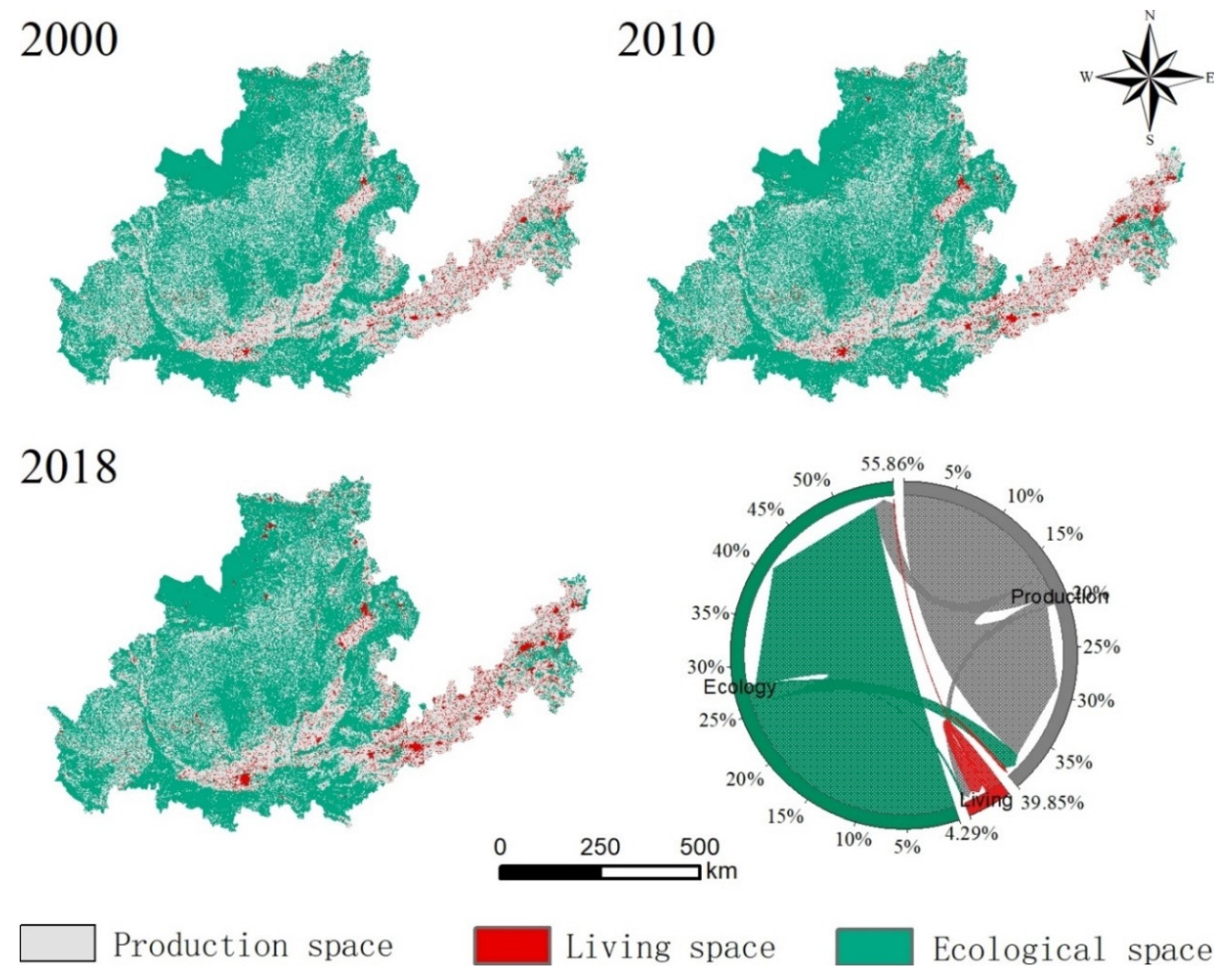
The Yellow River basin was mainly dominated by ecological space, with the percentage of ecological space being 55.73%, 55.97%, and 55.99% in 2000, 2010, and 2018, respectively, showing an increasing trend (Figure 3). The northwestern and southern parts of the study area were relatively less densely populated and had a lower level of urbanization and were therefore dominated by ecological space. The percentage of production space was 40.79%, 39.38%, and 38.91% in 2000, 2010, and 2018, respectively, showing a decreasing trend. Production space was mainly located in the eastern coastal areas of the study area, which have better water and heat conditions and are also conducive to crop growth. The region is economically developed, highly urbanized, with a high level of human activity and is a major industrial center and food producer.. The percentage of living space increased from 3.48% in 2000 to 5.10% in 2018. Spatially, living space was mainly distributed around the main cities in the study area, showing a tendency to spread outwards. The chord diagram suggests the scale of transfer of different land uses. The direction shown by the arrow represents the direction of transfer of the land, and the width of the arrow represents the proportion of the area transferred (Figure 3). According to the area conversion of PLES from 2000 to 2018, the largest area of production land was converted outwards, with a total of 35,300 km2, of which 10,800 km2 was converted to living land and 24,500 km2 was converted to ecological land. The smallest area of living land was converted outwards, with a total of 3720 km2, of which 3280 km2 was converted to production land and 433 km2 to ecological land. Ecological land converted mainly into productive land was 21,500 km2, while converted into living land was 1940 km2.
3.2. ES Supply and Demand Change and Mismatches
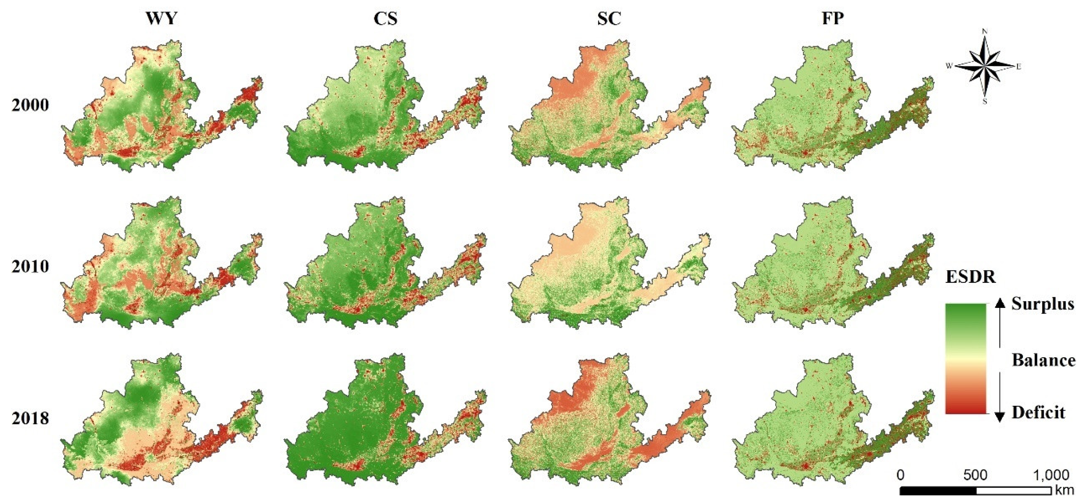
3.2.1. Water Yield Service
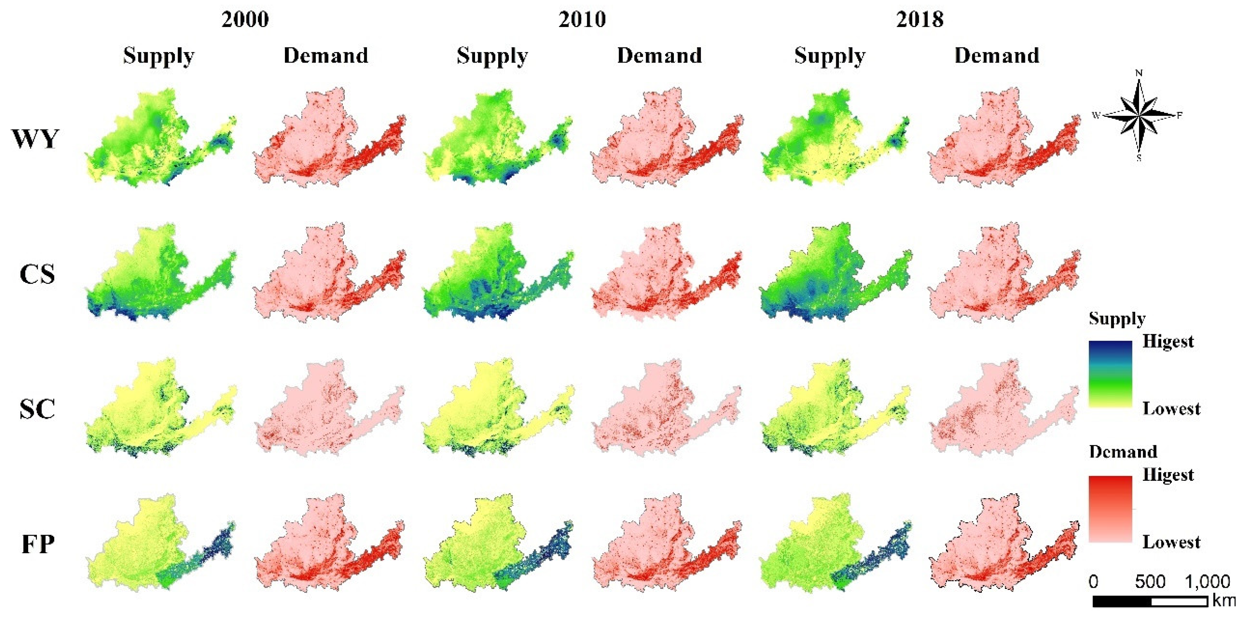
Over the entire period, the total water yield service supply exceeded demand, with surpluses of 47.72 billion m3, 60.31 billion m3, and 41.88 billion m3 in 2000, 2010, and 2018, respectively (Table 2). Water yield service supply in 2000, 2010, and 2018 was 72.32 billion m3, 84.63 billion m3, and 66.90 billion m3, respectively, showing a trend of increase followed by a decrease. The water demand increased significantly from 24.60 billion m3 in 2000 to 25.02 billion m3 in 2018, an increase of 1.69%.
Water yield service supply was strongly influenced by precipitation and evapotranspiration, while water demand was influenced by population density and industrial structure. Precipitation anomalies can increase the uncertainty of the spatial match of water yield service. Although there was an overall surplus of water service, the spatial distribution of water yield service supply and demand also showed a mismatch (Figure 4). The southern and eastern parts of the study area were the main areas of water yield service supply (Figure 5), but the deficit situation of the water yield service was still significant due to the dense population and agricultural development of the area, which means that there is a huge demand for water resources. Due to the lower water yield service supply in 2018, this has resulted in a significant deficit in water yield service in the South East, with the shortfall areas mainly in the city center.
3.2.2. Carbon Sequestration Service
Carbon sequestration service supply has shown an increasing trend, from 134.45 million tons in 2000 to 235.76 million tons in 2018, an increase of 75.35% (Table 2). However, the growth in the carbon sequestration service supply did not cause surpluses. Carbon sequestration demand in 2000, 2010, and 2018 was 134.45 million tons, 210.75 million tons, and 235.76 million tons, respectively, and the carbon sequestration demand in 2010 and 2018 exceeded the carbon sequestration supply with a deficit of 29.66 million tons and 49.48 million tons, respectively, with an upward trend.
According to the spatial distribution of carbon sequestration service supply and demand (Figure 4), higher carbon sequestration service supply was mainly concentrated in the south, showing an increasing trend, followed by a decreasing trend. Carbon sequestration supply in the north-western region was relatively low and shows an increasing trend. Higher carbon sequestration service demand was mainly in the main urban area downstream of the study but showed a decreasing trend from 2000 to 2018. There was a clear spatial mismatch in sequestration service (Figure 5), with increased surpluses in the central and western regions of the study area and relatively significant deficits in the eastern regions. The main urban areas around the study area showed a significant deficit in carbon sequestration service, with Zhengzhou showing an increase in the deficit position in 2018.
3.2.3. Soil Conservation Service
From 2000 to 2018, soil conservation service supply exceeded the demand, and both showed an increasing trend (Table 2). The surplus of soil conservation services increased significantly from 3.52 billion tons in 2000 to 5.6 billion tons in 2010 and 4.67 billion tons in 2018. Soil conservation services, as an in-situ service, i.e., one that is generated in situ and benefits in situ, have an aggregate surplus that hardly offsets their spatial mismatch.
In terms of the spatial distribution of the soil conservation services ESDR, the deficit areas were concentrated in the north-central region of the study area and the downtown area in the east (Figure 4). The spatial mismatch in soil conservation services was mainly due to: (1) the north-central region being a loess plateau area, which is very weak for soil and water conservation due to the undulating terrain, loose soil, and poor vegetation cover; (2) the eastern city center area, with strong human activity and high population density in the area, which has led to a reduction in vegetation area. The land-use types are mainly urban land, rural settlements, and other construction lands, which have a poor soil conservation capacity, thus leading to a deficit in soil conservation services.
3.2.4. Grain Production Service
Grain production service increased from 125.54 million tons in 2000 to 214.51 million tons in 2018, an increase of 70.87%. During the same period, grain production demand exhibited an increase of 14.24% from 51.30 million tons in 2000 to 58.62 million tons in 2018 (Table 2). Thus, there was a clear surplus for grain production service, and this surplus showed an increasing trend, from 74.23 million tons in 2000 to 155.90 million tons in 2018.
Despite the overall surplus in grain production service, there were still some spatially mismatched centers (Figure 5). The southeastern part of the study area has relatively good hydrothermal conditions and is a major grain producer, hence the high grain supply. At the same time, the grain demand was relatively high due to the high level of human activity and the relatively high population density in the area. The region’s grain production service showed a surplus, indicating that its production capacity was greater than its consumption capacity.
3.3. Influence of PLES Changing on ESDR
3.3.1. Influence of Production Space Changing on ESDR
There was a significant negative impact of production space on the ESDR for carbon sequestration service, soil conservation service, and water yield service during 2000–2018 (p < 0.01). The production space explained most of the variance in ESDR for carbon sequestration services, soil conservation services, and water production services, at 87%, 84%, and 48%, respectively (Figure 6a). For the carbon sequestration service, when the production space ratio exceeded 62.83%, the carbon sequestration service swas in deficit. Therefore, to ensure that the carbon sequestration service supply is greater than the demand, it is necessary to ensure that the ratio of production space is less than 62.83%. For the soil conservation service, the range was 0–98.73%. For the water yield service, there was no significant threshold effect due to the limited influence of production space (k = −0.02). Production space had a significant positive effect on the ESDR of grain production service and explained most of the variation in the ESDR for the grain supply service, at 89%. When the production space ratio exceeded 18.2%, grain production services supply exceeded the demand. In summary, it is necessary to ensure that the production space ratio in the study area is between 18.2% and 62.83% to ensure that all ecosystem services are in surplus.
3.3.2. Influence of Living Space Changing on ESDR
Living space had a significant negative influence (p < 0.01) on water yield service, grain production service, and carbon sequestration service (Figure 6c). For water production services, when the ratio of living space was greater than 31.35%, there was a deficit. This means that the water yield service supply was greater than the demand if the ratio of living space was less than 31.35%. For the carbon sequestration service and grain production service, this threshold was 15.68% and 44.39%, respectively.
Although the ESDR of living space on soil conservation services was negative, the trend was not strong (k = −0.01) and explained only part of the variation in soil conservation services (R2 = 0.45). The influence of the living space ratio was not significant, i.e., the soil conservation service was in surplus for any value of the living space ratio between 0–100%. In summary, the living space ratio between 0–15.68% is needed to ensure that all ecosystem services are in surplus in the study area. Due to the limited number of ES selected in this study, this resulted in a significant negative effect of living space on all ES. For some ES, such as landscape aesthetics, there is a dependence on living space, and too little living space will inevitably affect the supply of these ES.
3.3.3. Influence of Ecological Space Changing on ESDR
Ecological space had a significant positive influence on water yield service, soil conservation service, and carbon sequestration service during the period 2000–2018 (Figure 6b). Ecological space explained most of the variation in the ESDR for the soil conservation service and carbon sequestration service, at 78% and 86%, respectively. When the ecological space ratio was less than 29.79%, the carbon sequestration service was a deficit. This threshold did not exist for water yield service or soil conservation service. The ESDR of ecological space on grain production service was negative (p < 0.01). When the ecological space ratio was greater than 88.61%, there was a deficit in the grain production service. In summary, an ecological space ratio of 29.79% to 88.61% is needed to ensure that all ecosystem services are in surplus. However, this does not mean that ecological space can be expanded indefinitely, as too much ecological space can squeeze the original production space and lead to a deficit in grain production service.
4. Discussion
4.1. Identification of Optimization Directions in PLES
The ternary phase diagram can visually represent the ratio of PLES in any region, where the endpoints of the triangle indicate a production/living/ecological space ratio of 100% (Figure 7). According to the threshold value of the impact of PLES on the ES supply and demand imbalance, when the ratio of living space is less than 15.68%, the ratio of production space is between 18.2 and 62.83%, and the ratio of ecological space is between 29.79% and 88.61%, while the ES involved in this study are all in surplus. Accordingly, an ideal area, i.e., an area that does not need to be optimized, can be obtained. When the projection of an area falls within the ideal area, it means that this type of area does not need to be optimized, while the rest of the area needs to be optimized to varying degrees, depending on its location. The PLES of a region can be adjusted according to the range in the diagram where the ratio of PLES of any region falls. The greater the distance from the ideal area, the greater the area of change required in the land use pattern of the region.
The size of the ideal area is usually related to the ES selected. The more ES selected, the smaller the ideal area will be in response, meaning that more area will need to be adjusted. The ES can therefore be adjusted in the actual management process to suit the needs of the policymaker accordingly.
4.2. Optimization Measures and Policy Recommendations at Different Scales
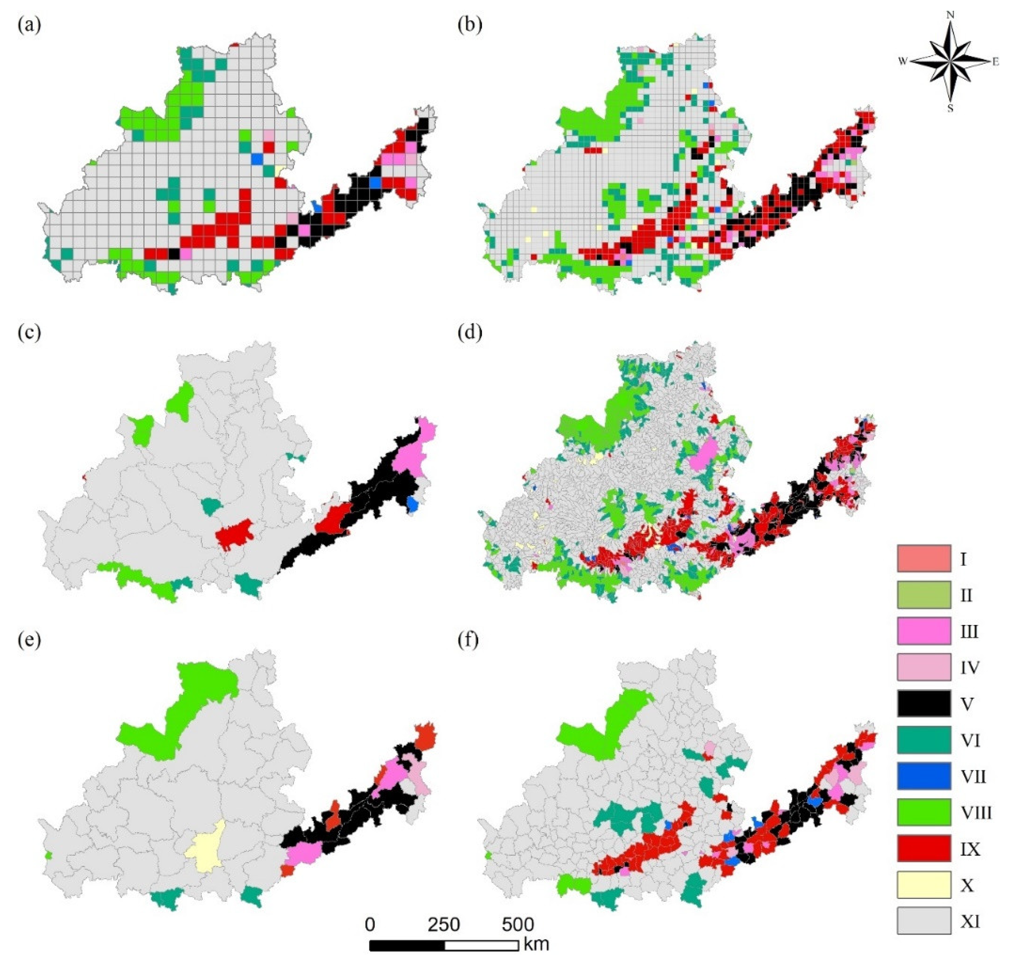
The distribution of PLES was highly spatially heterogeneous, which led to a spatial mismatch in ES. Therefore, the PLES optimization should be coupled with optimization measures at different scales to determine the best measures for ecosystem service management. In this study, the ratios of PLES at different scales were counted, and this was used to obtain optimization measures at multiple scales (Figure 8).
At the grid-scale, there was too much ecological space and not enough production space in the north-western part of the study area, and there is a need for conversion of ecological to production space, such as converting unused land in the area to industrial land. The central part of the study area had too much production space and not enough ecological space, so there is a need to convert the production land in the area to ecological land, such as implementing a system of returning farmland to forest or converting farmland unsuitable for cultivation to forest land. The eastern part of the study area, i.e., the lower reaches of the Yellow River Basin, was mainly characterized by an excess of living space and production space and a shortage of ecological space, so it is necessary to shift the production/living space towards ecological space, increasing the ratio of ecological space and reducing living space. For example, increase the woodland and grassland and reduce the rate of urbanization development. At the primary watershed scale, most of the Midwest was in the ideal mode of PLES, i.e., it did not need to be optimized. There was an excess of productive space in the eastern region and an excess of living space in the coastal region. At the secondary watershed scale, the central and western regions of the study area had more watersheds that need to be optimized, and they behaved in much the same way spatially as at the grid-scale. At the city scale, Erdos had too much ecological space and not enough production space, while Weinan had too much production space. At the county scale, some counties in the central region showed a shortage of production space, while others showed an excess of production space and a shortage of ecological space, implying that production space was not evenly distributed at the county scale in the region.
In conclusion, as the statistical scale increases, there is a general trend towards fewer areas in need of spatial optimization. The main problem in the north-western part of the study area was that there was too much ecological space and not enough production space. Therefore, it is necessary to increase the area of production land in the region, and as the region is also the main area of the Loess Plateau and undertakes important functions of soil and water conservation, the area of regional terraces and industrial land can be increased appropriately. The central part of the study area showed an uneven distribution of production space and a lack of ecological space, so it is necessary to adjust the distribution of production space at several scales to ensure that it is in a reasonable range, while the ratio of ecological land, such as woodland and grassland, can be increased appropriately. The eastern part of the study area had a large ratio of production space and living space area and too little ecological space. Therefore, it is necessary to reduce and harmonize production and living space, while increasing the right amount of ecological space, such as green space and woodland. Here, the direction of the PLES adjustment is mainly explained, which in practice it can be quantified according to the difference between the PLES ratio of a region and the ideal region.
4.3. Limitations and Future Research Directions
This study aims to optimize the PLES with the objective that all ecosystem services can be in surplus as far as possible and proposes corresponding optimizations at multiple scales. This study can provide a basis for decision-making on regional land use management and rational allocation of resources. However, there are some problems with this study. Firstly, in assessing ES, this study used several models, such as the RUSLE model, water balance equation, and CASA model, where differences in data sources and calculation methods can lead to differences in results. Although there are still no effective solutions to these problems, these methods are still widely used [54,55]. Additionally, due to the lack of data and the limitations of ecosystem service models, only the supply and demand of four ES were assessed, which is not comprehensive for the complete management of ES. More ES assessments should be added in future studies. In addition, the use of land-use types for the classification of PLES is a more straightforward method [56]. However, this approach ignores the complex multifunctionality of land. For example, arable land (paddy and dryland) is uniformly classified as production space without taking into account its ecological characteristics. Finally, the issue of scale is also one of the problems studied in this study, with spatial correlation results varying with unit size (grid cell or grain size) [26,57]. In this study, the identification of thresholds was based on the grid-scale using a hierarchical statistical approach. Random points, various grid cell sizes, and basin units should be selected in subsequent studies to explore the differences in the impact of PLES on the ES supply and demand imbalance.
5. Conclusions
Based on various models and methods, this study quantified the mismatch of supply and demand for the four ES in the Yellow River Basin and explores how the spatial pattern of PLES can be adjusted to keep the ES in supply and demand balance. The results show that in 2000, 2010, and 2018, the total supply of the three ecosystem services in the Yellow River Basin was greater than the total demand, except for carbon sequestration services. Along with the implementation of revegetation projects and the establishment of ecological reserves in the region, the supply of many ecosystem services was on the rise. However, increased urbanization and over-concentration of population and economy resulted in a serious spatial mismatch between supply and demand for all four ecosystem services, especially in the major urban centers. The spatial mismatch in ES can be effectively reduced by optimizing the PLES, e.g., increasing the production spatial ratio can effectively increase the supply of grain production service and alleviate the contradiction between supply and demand of grain production service in certain regions. This study provides an optimization objective for the PLES optimization of other regions by providing an ideal region in the ternary phase diagram, i.e., one that can ensure that multiple ES are in surplus at the same time. The direction of optimization of other areas is determined by their relative position to the ideal area, and the amount of adjustment of PLES can be determined by the difference from the ideal area. The PLES optimization framework proposed in this study is very flexible, as reflected in the choice of ES and multi-scale optimization proposals, which can effectively reduce the deficit problem of regional ES in the process of practical application.
Author Contributions
Conceptualization, X.F.; data curation, X.W.; formal analysis, J.M.; funding acquisition, X.W.; investigation, X.F.; methodology, X.F. and J.Z.; resources, X.W.; supervision, X.W.; visualization, X.F., J.Z. and J.M.; writing—original draft, X.F. All authors have read and agreed to the published version of the manuscript.
Funding
This research was funded by the National Key Research and Development Plan of China (2016YFC0501603), the Chinese Academic of Sciences, the Strategic Priority Research Program of the Chinese Academy of Sciences (XDA2002040201).
Conflicts of Interest
The authors declare no conflict of interest.
References
- Haas, J.; Ban, Y. Urban growth and environmental impacts in Jing-Jin-Ji, the Yangtze, River Delta and the Pearl River Delta. Int. J. Appl. Earth Obs. Geoinf. 2014, 30, 42–55. [Google Scholar] [CrossRef]
- Allington, G.R.; Li, W.; Brown, D.G. Urbanization and environmental policy effects on the future availability of grazing re-sources on the Mongolian Plateau: Modeling socio-environmental system dynamics. Environ. Sci. Policy 2017, 68, 35–46. [Google Scholar] [CrossRef] [Green Version]
- Foley, J.A.; DeFries, R.; Asner, G.P.; Barford, C.; Bonan, G.; Carpenter, S.R.; Chapin, F.S.; Coe, M.T.; Daily, G.C.; Gibbs, H.K.; et al. Global Consequences of Land Use. Science 2005, 309, 570–574. [Google Scholar] [CrossRef] [PubMed] [Green Version]
- Wang, J.; He, T.; Lin, Y. Changes in ecological, agricultural, and urban land space in 1984–2012 in China: Land policies and regional social-economical drivers. Habitat Int. 2018, 71, 1–13. [Google Scholar] [CrossRef]
- Liu, Y.S. Introduction to land use and rural sustainability in China. Land Use Policy 2018, 74, 1–4. [Google Scholar] [CrossRef]
- Ma, W.; Jiang, G.; Li, W.; Zhou, T.; Zhang, R. Multifunctionality assessment of the land use system in rural residential areas: Confronting land use supply with rural sustainability demand. J. Environ. Manag. 2019, 231, 73–85. [Google Scholar] [CrossRef]
- Thorne, J.H.; Santos, M.J.; Bjorkman, J.H. Regional Assessment of Urban Impacts on Landcover and Open Space Finds a Smart Urban Growth Policy Performs Little Better than Business as Usual. PLoS ONE 2013, 8, e65258. [Google Scholar] [CrossRef] [PubMed]
- Li, Y.; Li, Y.; Westlund, H.; Liu, Y. Urban-rural transformation in relation to cultivated land conversion in China: Implications for optimizing land use and balanced regional development. Land Use Policy 2015, 47, 218–224. [Google Scholar] [CrossRef]
- Deines, J.M.; Schipanski, M.E.; Golden, B.; Zipper, S.C.; Nozari, S.; Rottler, C.; Guerrero, B.; Sharda, V. Transitions from irri-gated to dryland agriculture in the Ogallala Aquifer: Land use suitability and regional economic impacts. Agric. Water Manag. 2020, 233, 106061. [Google Scholar] [CrossRef]
- Sommer, W.; Valstar, J.; Leusbrock, I.; Grotenhuis, T.; Rijnaarts, H. Optimization and spatial pattern of large-scale aquifer thermal energy storage. Appl. Energy 2015, 137, 322–337. [Google Scholar] [CrossRef]
- Lin, G.; Jiang, D.; Fu, J.; Cao, C.; Zhang, D. Spatial Conflict of Production-Living-Ecological Space and Sustaina-ble-Development Scenario Simulation in Yangtze River Delta Agglomerations. Sustainability 2020, 12, 2175. [Google Scholar] [CrossRef] [Green Version]
- Tian, F.; Li, M.; Han, X.; Liu, H.; Mo, B. A Production–Living–Ecological Space Model for Land-Use Optimisation: A case study of the core Tumen River region in China. Ecol. Model. 2020, 437, 109310. [Google Scholar] [CrossRef]
- Costanza, R.; De Groot, R.; Braat, L.; Kubiszewski, I.; Fioramonti, L.; Sutton, P.; Farber, S.; Grasso, M. Twenty years of ecosystem services: How far have we come and how far do we still need to go? Ecosyst. Serv. 2017, 28, 1–16. [Google Scholar] [CrossRef]
- Pharo, E.; Daily, G.C. Nature’s Services: Societal Dependence on Natural Ecosystems. Bryology 1998, 101, 475. [Google Scholar] [CrossRef] [Green Version]
- Palmer, M.A.; Filoso, S. Restoration of Ecosystem Services for Environmental Markets. Science 2009, 325, 575–576. [Google Scholar] [CrossRef] [Green Version]
- Fu, B.; Wang, S.; Su, C.; Forsius, M. Linking ecosystem processes and ecosystem services. Curr. Opin. Environ. Sustain. 2013, 5, 4–10. [Google Scholar] [CrossRef]
- Wu, X.; Liu, S.; Zhao, S.; Hou, X.; Xu, J.; Dong, S.; Liu, G. Quantification and driving force analysis of ecosystem services supply, demand and balance in China. Sci. Total Environ. 2019, 652, 1375–1386. [Google Scholar] [CrossRef]
- Peng, J.; Wang, X.; Liu, Y.; Zhao, Y.; Xu, Z.; Zhao, M.; Qiu, S.; Wu, J. Urbanization impact on the supply-demand budget of ecosystem services: Decoupling analysis. Ecosyst. Serv. 2020, 44, 101139. [Google Scholar] [CrossRef]
- Zhao, W.; Liu, Y.; Daryanto, S.; Fu, B.; Wang, S.; Liu, Y. Metacoupling supply and demand for soil conservation service. Curr. Opin. Environ. Sustain. 2018, 33, 136–141. [Google Scholar] [CrossRef]
- Fu, B.; Li, Y. Bidirectional coupling between the Earth and human systems is essential for modeling sustainability. Natl. Sci. Rev. 2016, 3, 397–398. [Google Scholar] [CrossRef] [Green Version]
- Bai, Y.; Zhuang, C.; Ouyang, Z.; Zheng, H.; Jiang, B. Spatial characteristics between biodiversity and ecosystem services in a human-dominated watershed. Ecol. Complex 2011, 8, 177–183. [Google Scholar] [CrossRef]
- Gao, Q.; Kang, M.; Xu, H.; Jiang, Y.; Yang, J. Optimization of land use structure and spatial pattern for the semi-arid loess hilly–gully region in China. Catena 2010, 81, 196–202. [Google Scholar] [CrossRef]
- Chen, J.; Jiang, B.; Bai, Y.; Xu, X.; Alatalo, J. Quantifying ecosystem services supply and demand shortfalls and mismatches for management optimisation. Sci. Total Environ. 2019, 650, 1426–1439. [Google Scholar] [CrossRef] [PubMed]
- Sun, Y.X.; Liu, S.L.; Shi, F.N.; An, Y.; Li, M.Q.; Liu, Y.X. Spatio-temporal variations and coupling of human activity intensity and ecosystem services based on the four-quadrant model on the Qinghai-Tibet Plateau. Sci. Total Environ. 2020, 743, 140721. [Google Scholar]
- Santos-Martín, F.; Zorrilla-Miras, P.; Palomo, I.; Montes, C.; Benayas, J.; Maes, J. Protecting nature is necessary but not sufficient for conserving ecosystem services: A comprehensive assessment along a gradient of land-use intensity in Spain. Ecosyst. Serv. 2019, 35, 43–51. [Google Scholar] [CrossRef]
- Peng, J.; Tian, L.; Liu, Y.; Zhao, M.; Hu, Y.; Wu, J. Ecosystem services response to urbanization in metropolitan areas: Thresholds identification. Sci. Total Environ. 2017, 607–608, 706–714. [Google Scholar] [CrossRef] [PubMed]
- Li, D.; Wu, S.; Liu, L.; Liang, Z.; Li, S. Evaluating regional water security through a freshwater ecosystem service flow model: A case study in Beijing-Tianjian-Hebei region, China. Ecol. Indic. 2017, 81, 159–170. [Google Scholar] [CrossRef]
- Ouyang, Z.; Zheng, H.; Xiao, Y.; Polasky, S.; Liu, J.; Xu, W.; Wang, Q.; Zhang, L.; Xiao, Y.; Rao, E.; et al. Improvements in ecosystem services from investments in natural capital. Science 2016, 352, 1455–1459. [Google Scholar] [CrossRef]
- Zhang, Z.; Peng, J.; Xu, Z.; Wang, X.; Meersmans, J. Ecosystem services supply and demand response to urbanization: A case study of the Pearl River Delta, China. Ecosyst. Serv. 2021, 49, 101274. [Google Scholar] [CrossRef]
- Burkhard, B.; Kroll, F.; Nedkov, S.; Müller, F. Mapping ecosystem service supply, demand and budgets. Ecol. Indic. 2012, 21, 17–29. [Google Scholar] [CrossRef]
- Wei, H.; Fan, W.; Wang, X.-C.; Lu, N.; Dong, X.; Zhao, Y.; Ya, X.; Zhao, Y. Integrating supply and social demand in ecosystem services assessment: A review. Ecosyst. Serv. 2017, 25, 15–27. [Google Scholar] [CrossRef]
- Woldeyohannes, A.; Cotter, M.; Biru, W.D.; Kelboro, G. Assessing Changes in Ecosystem Service Values over 1985–2050 in Response to Land Use and Land Cover Dynamics in Abaya-Chamo Basin, Southern Ethiopia. Land 2020, 9, 37. [Google Scholar] [CrossRef] [Green Version]
- Hasan, S.S.; Zhen, L.; Miah, G.; Ahamed, T.; Samie, A. Impact of land use change on ecosystem services: A review. Environ. Dev. 2020, 34, 100527. [Google Scholar] [CrossRef]
- Wilkerson, M.L.; Mitchell, M.G.; Shanahan, D.; Wilson, K.; Ives, C.D.; Lovelock, C.; Rhodes, J. The role of socio-economic factors in planning and managing urban ecosystem services. Ecosyst. Serv. 2018, 31, 102–110. [Google Scholar] [CrossRef]
- Cui, F.; Tang, H.; Zhang, Q.; Wang, B.; Dai, L. Integrating ecosystem services supply and demand into optimized management at different scales: A case study in Hulunbuir, China. Ecosyst. Serv. 2019, 39, 100984. [Google Scholar] [CrossRef]
- Feng, Q.; Zhao, W.; Fu, B.; Ding, J.; Wang, S. Ecosystem service trade-offs and their influencing factors: A case study in the Loess Plateau of China. Sci. Total Environ. 2017, 607–608, 1250–1263. [Google Scholar] [CrossRef] [PubMed]
- Knoke, T.; Paul, C.; Rammig, A.; Gosling, E.; Hildebrandt, P.; Härtl, F.; Peters, T.; Richter, M.; Diertl, K.H.; Castro, L.M. Ac-counting for multiple ecosystem services in a simulation of land-use decisions: Does it reduce tropical deforestation? Glob. Chang. Biol. 2020, 26, 2403–2420. [Google Scholar] [CrossRef] [PubMed] [Green Version]
- Zou, L.; Liu, Y.; Wang, J.; Yang, Y. An analysis of land use conflict potentials based on ecological-production-living function in the southeast coastal area of China. Ecol. Indic. 2021, 122, 107297. [Google Scholar] [CrossRef]
- Yang, Y.; Bao, W.; Liu, Y. Coupling coordination analysis of rural production-living-ecological space in the Beijing-Tianjin-Hebei region. Ecol. Indic. 2020, 117, 106512. [Google Scholar] [CrossRef]
- Lin, G.; Fu, J.; Jiang, D. Production–Living–Ecological Conflict Identification Using a Multiscale Integration Model Based on Spatial Suitability Analysis and Sustainable Development Evaluation: A Case Study of Ningbo, China. Land 2021, 10, 383. [Google Scholar] [CrossRef]
- Świąder, M.; Szewrański, S.; Kazak, J.K. Environmental Carrying Capacity Assessment—The Policy Instrument and Tool for Sustainable Spatial Management. Front. Environ. Sci. 2020, 8. [Google Scholar] [CrossRef]
- Li, Y.; Ye, H.; Sun, X.; Zheng, J.; Meng, D. Coupling Analysis of the Thermal Landscape and Environmental Carrying Capacity of Urban Expansion in Beijing (China) over the Past 35 Years. Sustainability 2021, 13, 584. [Google Scholar] [CrossRef]
- Ding, X.; Zheng, M.; Zheng, X. The Application of Genetic Algorithm in Land Use Optimization Research: A Review. Land 2021, 10, 526. [Google Scholar] [CrossRef]
- Baró, F.; Haase, D.; Gómez-Baggethun, E.; Frantzeskaki, N. Mismatches between ecosystem services supply and demand in urban areas: A quantitative assessment in five European cities. Ecol. Indic. 2015, 55, 146–158. [Google Scholar] [CrossRef] [Green Version]
- Xie, X.; Li, X.; Fan, H.; He, W. Spatial analysis of production-living-ecological functions and zoning method under symbiosis theory of Henan, China. Environ. Sci. Pollut. Res. 2021, 1–18. [Google Scholar] [CrossRef]
- Bai, P.; Liu, X.; Zhang, Y.; Liu, C. Assessing the Impacts of Vegetation Greenness Change on Evapotranspiration and Water Yield in China. Water Resour. Res. 2020, 56, 56. [Google Scholar] [CrossRef]
- Jia, X.; Fu, B.; Feng, X.; Hou, G.; Liu, Y.; Wang, X. The tradeoff and synergy between ecosystem services in the Grain-for-Green areas in Northern Shaanxi, China. Ecol. Indic. 2014, 43, 103–113. [Google Scholar] [CrossRef]
- Beven, K. A sensitivity analysis of the Penman-Monteith actual evapotranspiration estimates. J. Hydrol. 1979, 44, 169–190. [Google Scholar] [CrossRef]
- Mehring, M.; Ott, E.; Hummel, D. Ecosystem services supply and demand assessment: Why social-ecological dynamics matter. Ecosyst. Serv. 2018, 30, 124–125. [Google Scholar] [CrossRef]
- Luo, Y.; Lü, Y.; Fu, B.; Zhang, Q.; Li, T.; Hu, W.; Comber, A. Half century change of interactions among ecosystem services driven by ecological restoration: Quantification and policy implications at a watershed scale in the Chinese Loess Plateau. Sci. Total. Environ. 2019, 651, 2546–2557. [Google Scholar] [CrossRef] [Green Version]
- Renard, K.G. Predicting Soil Erosion by Water: A Guide to Conservation Planning with the Revised Universal Soil Loss Equation (RUSLE); United States Government Printing: Washington, DC, USA, 1997.
- Wischmeier, W.H.; Smith, D.D. Predicting Rainfall Erosion Losses: A Guide to Conservation Planning; Department of Agriculture, Science and Education Administration: Washington, DC, USA, 1978. [Google Scholar]
- Yu, H.; Xie, W.; Sun, L.; Wang, Y. Identifying the regional disparities of ecosystem services from a supply-demand perspective. Resour. Conserv. Recycl. 2021, 169, 105557. [Google Scholar] [CrossRef]
- Qin, K.; Lin, Y.-P.; Yang, X. Trade-Off and Synergy among Ecosystem Services in the Guanzhong-Tianshui Economic Region of China. Int. J. Environ. Res. Public Health 2015, 12, 14094–14113. [Google Scholar] [CrossRef]
- Abera, W.; Tamene, L.; Tibebe, D.; Adimassu, Z.; Kassa, H.; Hailu, H.; Mekonnen, K.; Desta, G.; Sommer, R.; Verchot, L. Characterizing and evaluating the impacts of national land restoration initiatives on ecosystem services in Ethiopia. Land Degrad. Dev. 2020, 31, 37–52. [Google Scholar] [CrossRef]
- Yu, S.-H.; Deng, W.; Xu, Y.-X.; Zhang, X.; Xiang, H.-L. Evaluation of the production-living-ecology space function suitability of Pingshan County in the Taihang mountainous area, China. J. Mt. Sci. 2020, 17, 2562–2576. [Google Scholar] [CrossRef]
- Chi, Y.; Zhang, Z.; Gao, J.; Xie, Z.; Zhao, M.; Wang, E. Evaluating landscape ecological sensitivity of an estuarine island based on landscape pattern across temporal and spatial scales. Ecol. Indic. 2019, 101, 221–237. [Google Scholar] [CrossRef]
Figure 1.
(a–c) Location, elevation, and 2018 land use of the study area.

Figure 2.
Optimization framework for production-living-ecological space.

Figure 3.
Structure and transition of production-living-ecological space in the Yellow River Basin from 2000 to 2018.
Figure 3.
Structure and transition of production-living-ecological space in the Yellow River Basin from 2000 to 2018.

Figure 4.
Spatial pattern of supply and demand for individual ecosystem services (ES) in the Yellow River Basin in 2000, 2008, and 2018. ES indicators are: WY—water yield; CS—carbon sequestration; SC—soil conservation; GP—grain production.
Figure 4.
Spatial pattern of supply and demand for individual ecosystem services (ES) in the Yellow River Basin in 2000, 2008, and 2018. ES indicators are: WY—water yield; CS—carbon sequestration; SC—soil conservation; GP—grain production.

Figure 5.
Spatial pattern of the ecosystem service supply-demand ratio in the Yellow River Basin in 2000, 2008, and 2018.
Figure 5.
Spatial pattern of the ecosystem service supply-demand ratio in the Yellow River Basin in 2000, 2008, and 2018.

Figure 6.
Influence of production space ratio, living space ratio, and ecological space ratio on ESDR in the Yellow River Basin. (a). Production space ratio (b). Ecological space ratio (c). Living space ratio.
Figure 6.
Influence of production space ratio, living space ratio, and ecological space ratio on ESDR in the Yellow River Basin. (a). Production space ratio (b). Ecological space ratio (c). Living space ratio.

Figure 7.
Ternary phase diagram of production-living-ecological space.

Figure 8.
Optimization of production-living-ecological space on multiple scales ((a). the 40 × 40 km grid scale; (b). the 20 × 20 km grid scale; (c). the primary catchment scale; (d). the secondary catchment scale; (e). the city scale; (f). the county scale. TheⅠto XI corresponds to Figure 7 numbering).


Table 1.
Production-living-ecological space classification in the Yellow River Basin.
| LUCC Classification System | |
|---|---|
| Production space | Paddy land (11), dry land (12), transport, industrial, and mining construction land (53) |
| Living space | Urban sites (51), rural settlements (52) |
| Ecological space | Wooded land (21), shrubland (22), high cover grassland (31), medium cover grassland (32), rivers and canals (41), lakes (42), reservoir ponds (43), open woodland (23), other woodlands (24), permanent glacial snow (44), mudflats (46) cover grassland (33), sandy land (61), gobi 62), saline land (63), marshland (64), bare land (65), bare rocky ground (66) |
Table 2.
Ecosystem services supply and demand in the Yellow River Basin in 2000, 2010, and 2018.
| Year | Water Yield (m3/km2/a) | Carbon Sequestration (tc/km2/a) | Soil Conservation (t/ha/a) | Grain Production (t/km2/a) | ||||
|---|---|---|---|---|---|---|---|---|
| Supply | Demand | Supply | Demand | Supply | Demand | Supply | Demand | |
| 2000 | 128,995.41 | 43,882.20 | 239.82 | 134.75 | 71.80 | 8.96 | 223.92 | 91.52 |
| 2010 | 150,950.80 | 43,368.23 | 375.92 | 428.83 | 110.53 | 10.58 | 326.43 | 98.28 |
| 2018 | 119,332.21 | 44,622.76 | 420.52 | 508.78 | 90.39 | 6.92 | 382.62 | 104.55 |
Publisher’s Note: MDPI stays neutral with regard to jurisdictional claims in published maps and institutional affiliations. |
© 2021 by the authors. Licensee MDPI, Basel, Switzerland. This article is an open access article distributed under the terms and conditions of the Creative Commons Attribution (CC BY) license (https://creativecommons.org/licenses/by/4.0/).
Share and Cite
MDPI and ACS Style
Fu, X.; Wang, X.; Zhou, J.; Ma, J. Optimizing the Production-Living-Ecological Space for Reducing the Ecosystem Services Deficit. Land 2021, 10, 1001. https://0-doi-org.brum.beds.ac.uk/10.3390/land10101001
AMA Style
Fu X, Wang X, Zhou J, Ma J. Optimizing the Production-Living-Ecological Space for Reducing the Ecosystem Services Deficit. Land. 2021; 10(10):1001. https://0-doi-org.brum.beds.ac.uk/10.3390/land10101001
Chicago/Turabian StyleFu, Xinxin, Xiaofeng Wang, Jitao Zhou, and Jiahao Ma. 2021. "Optimizing the Production-Living-Ecological Space for Reducing the Ecosystem Services Deficit" Land 10, no. 10: 1001. https://0-doi-org.brum.beds.ac.uk/10.3390/land10101001
Note that from the first issue of 2016, this journal uses article numbers instead of page numbers. See further details here.