Evaluation of the Accuracy of Four Digital Methods by Linear and Volumetric Analysis of Dental Impressions


 , ,
, ,
Abstract
:1. Introduction
2. Materials and Methods
2.1. Master Model Molding
2.2. Reference Digitalization
2.3. Impression Scanning
2.4. Data Analysis with Commercial Software
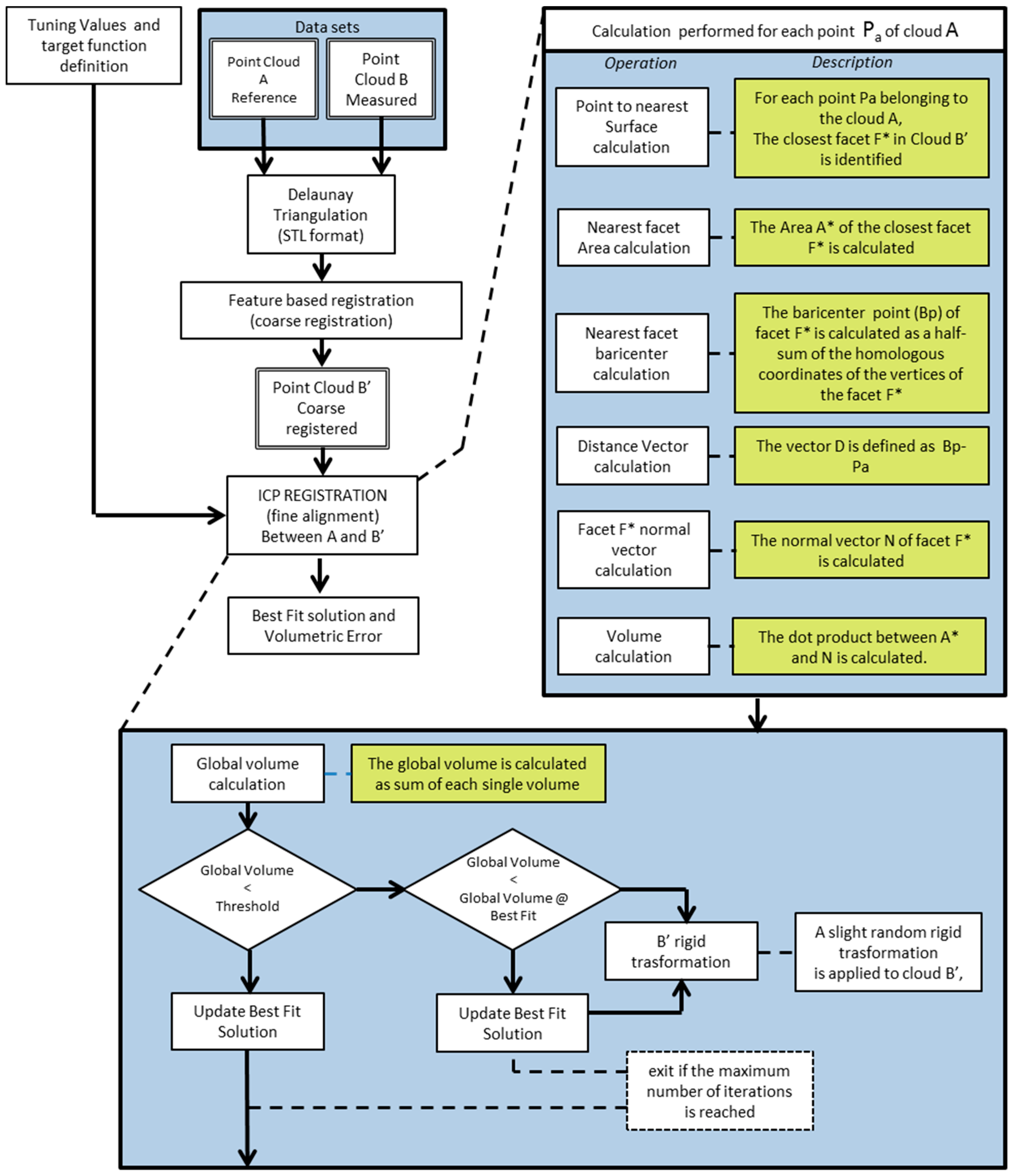
2.5. Data Analysis with Proposed Algorithm: MATLAB Environment
2.6. Statistical Analysis
3. Results
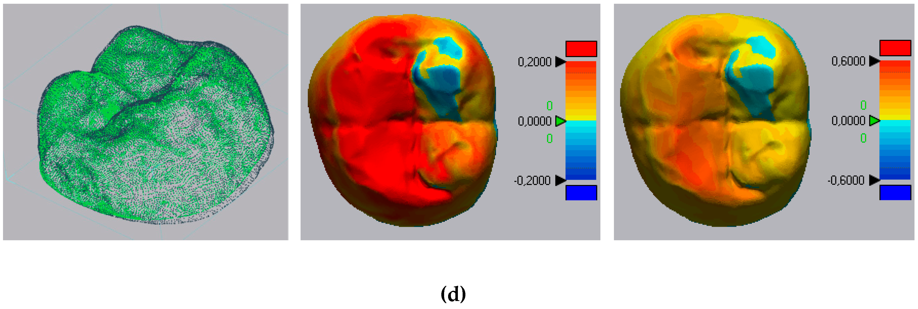
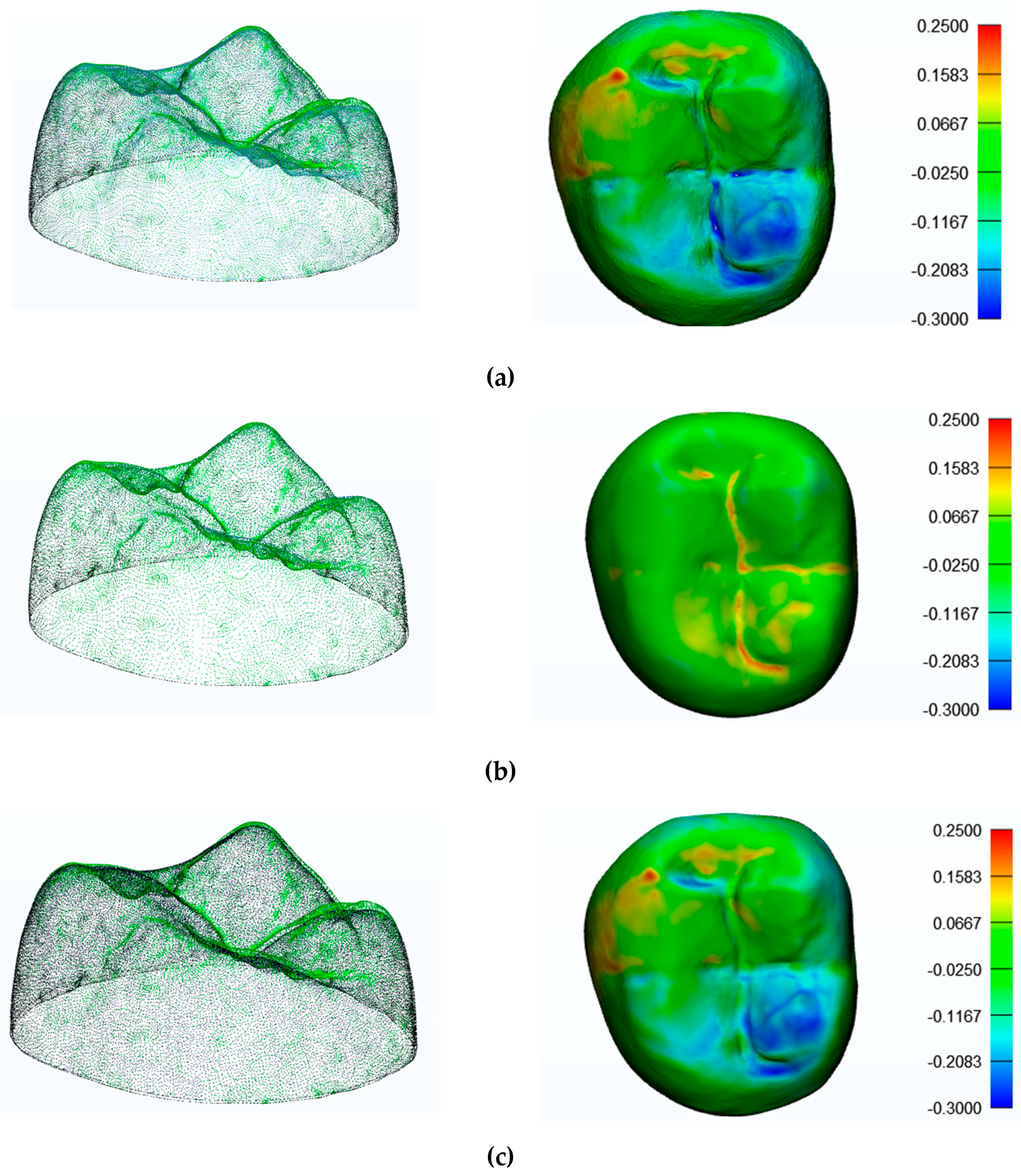
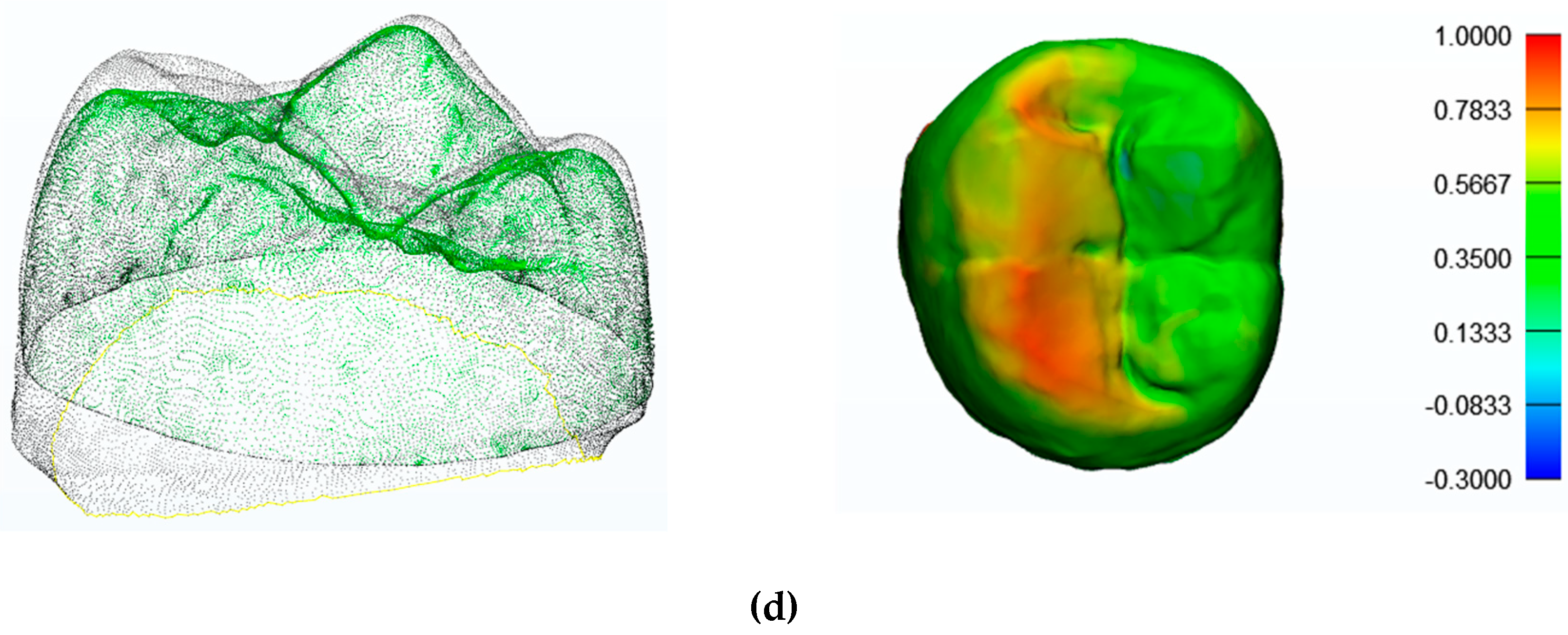
3.1. Comparison of Geometries with Commercial Software
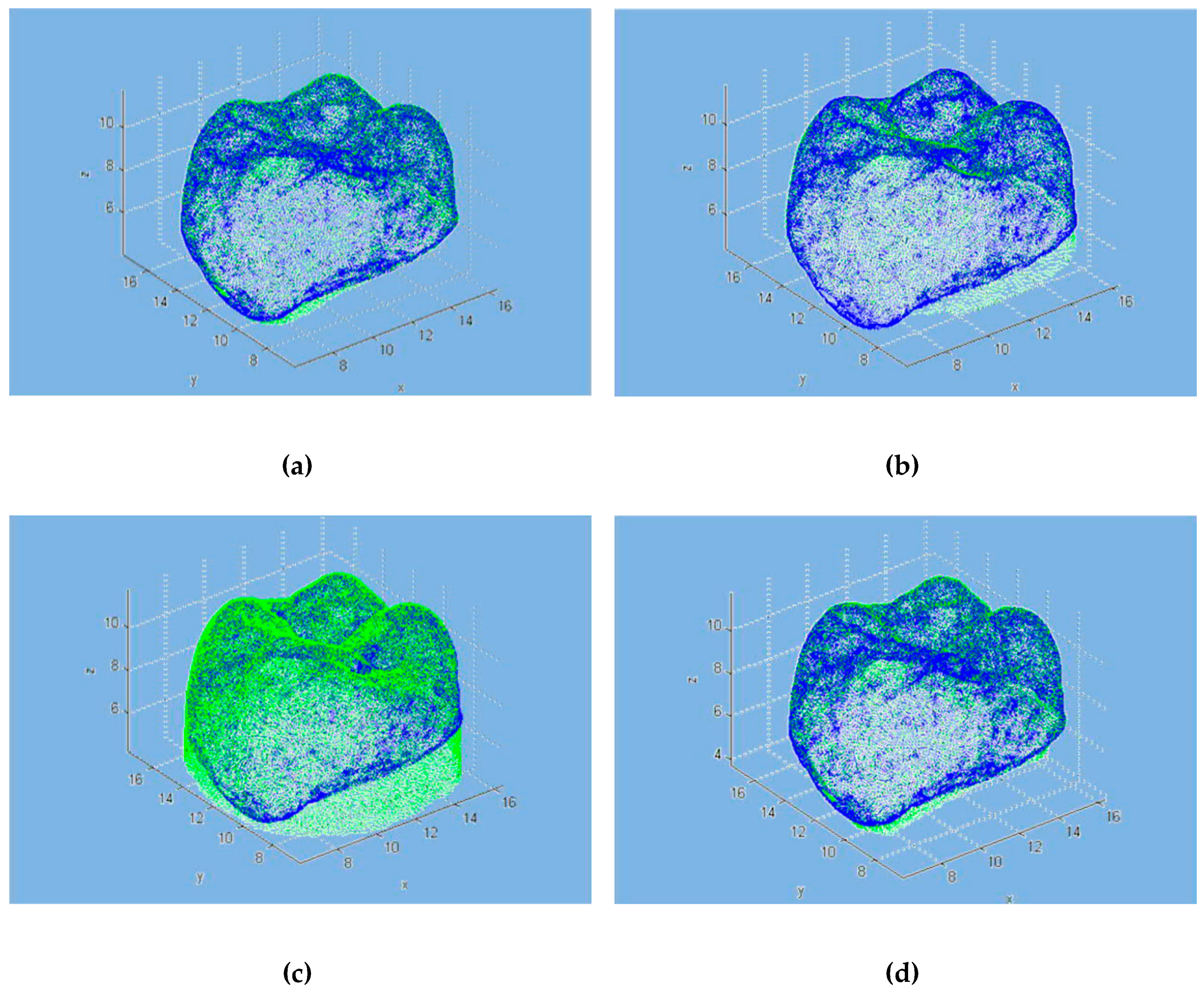
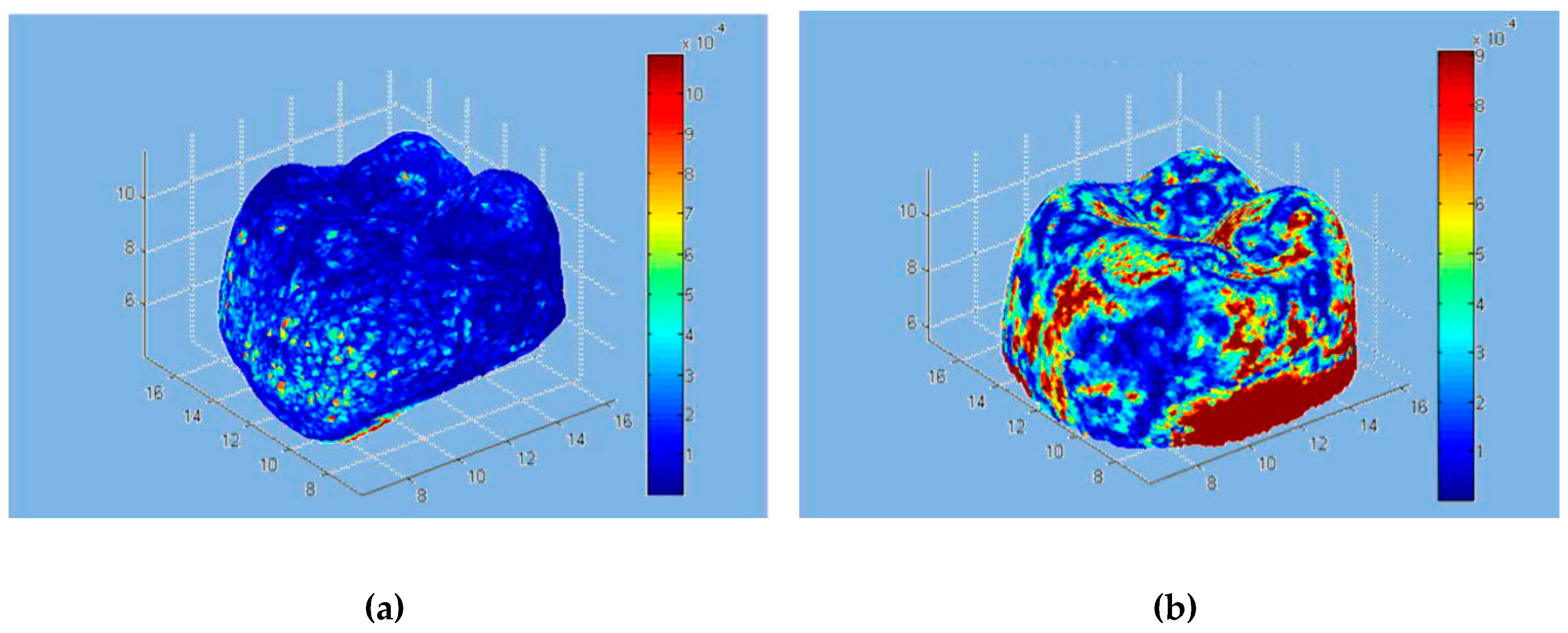
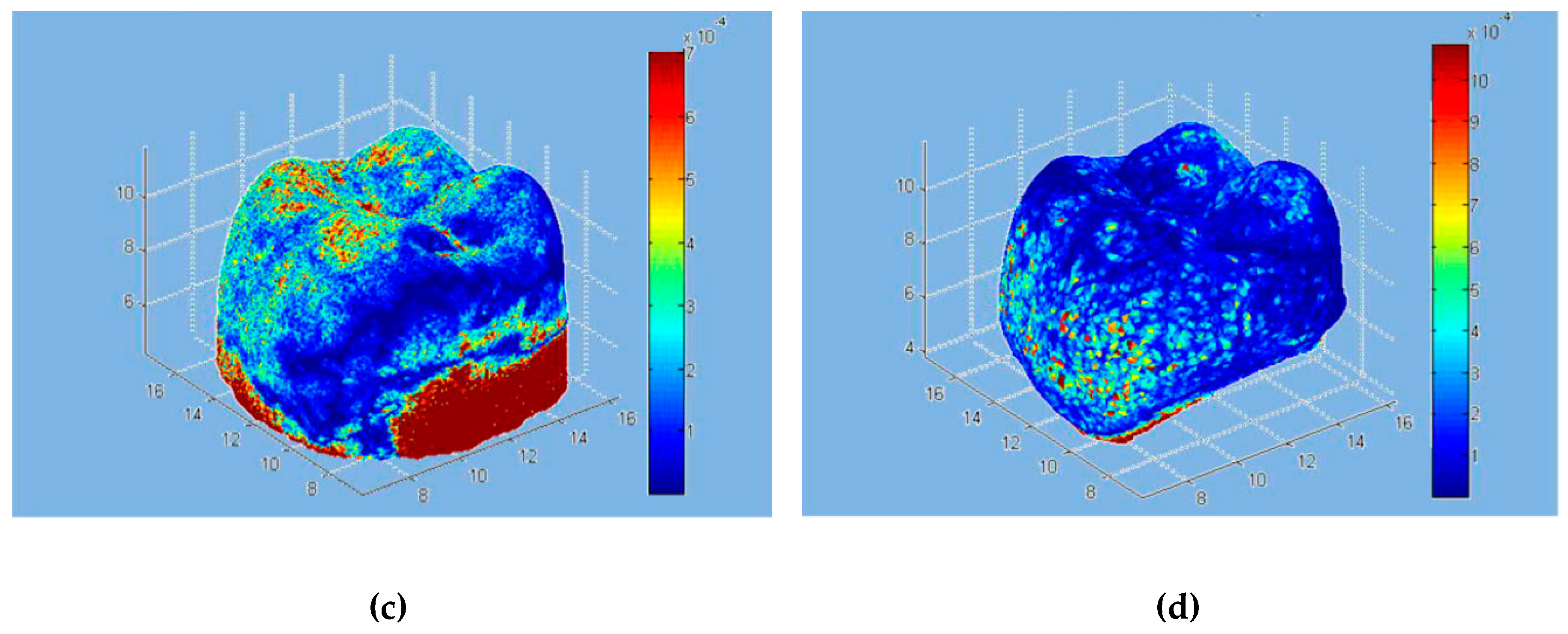
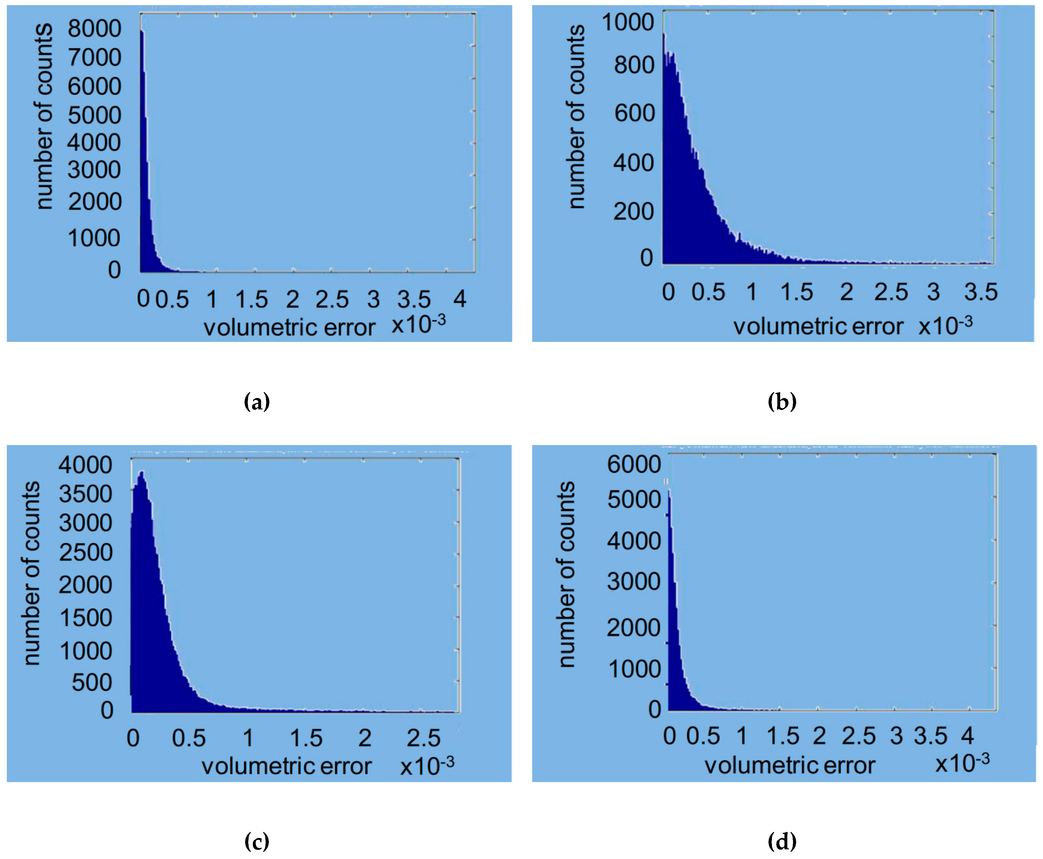
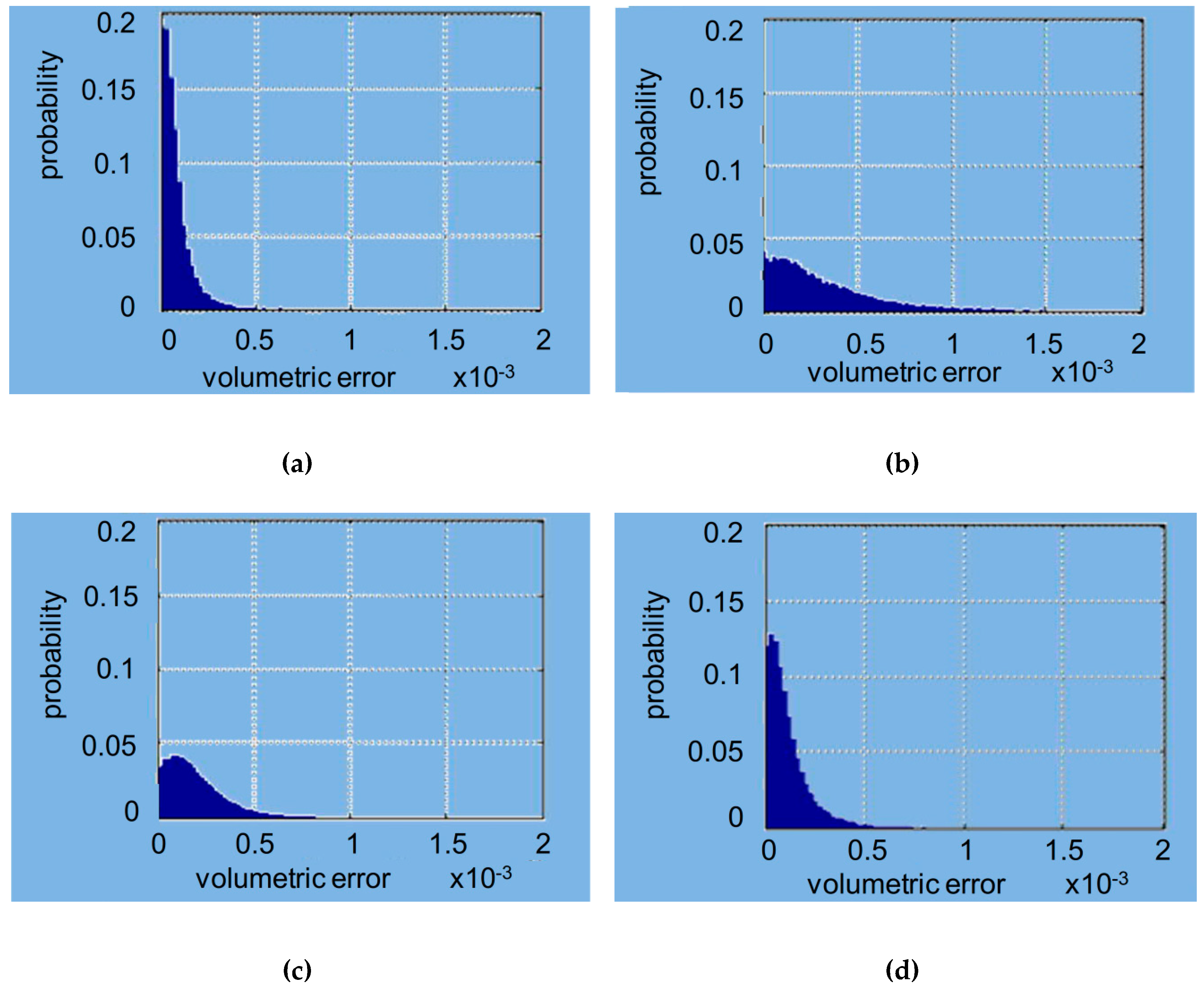
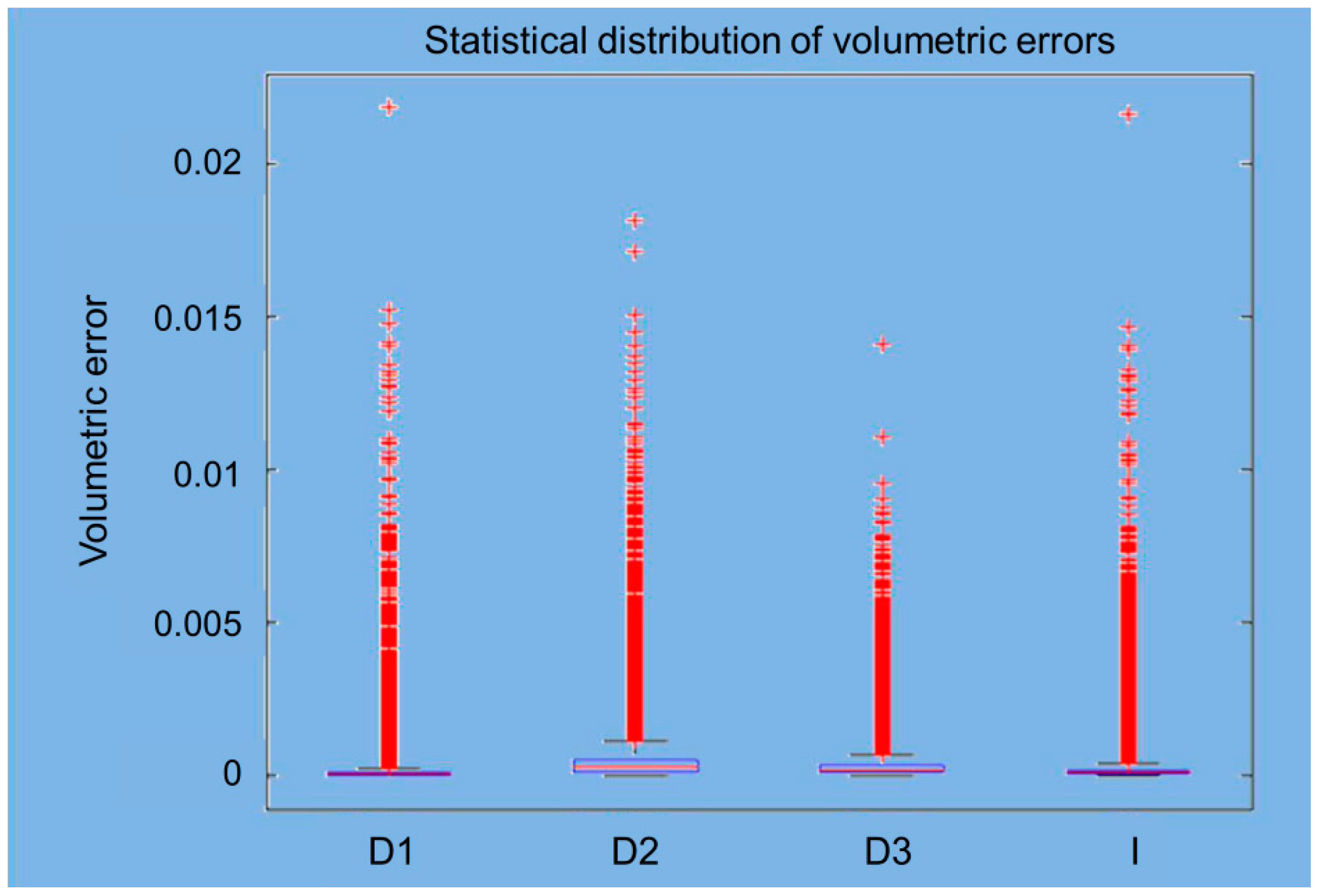
3.2. Comparison of Geometries with MATLAB Custom Algorithm Results
4. Discussion
5. Conclusions
Author Contributions
Funding
Conflicts of Interest
Appendix A

| Sample n° | Scanner D1: Min [mm] 3-matic | Scanner D1: Max [mm] 3-matic | Scanner D1: Median [mm] 3-matic | Scanner D1: Mean [mm] 3-matic | Scanner D1: SD[mm] 3-matic | Scanner D1: Min [mm] Geomagic | Scanner D1: Max [mm] Geomagic | Scanner D1: Mean [mm] Geomagic | Scanner D1: SD [mm] Geomagic |
|---|---|---|---|---|---|---|---|---|---|
| 1 | −0.2885 | 0.0115 | −0.0628 | −0.0363 | 0.0814 | −0.38545406 | 0.276725124 | −0.04893728 | 0.055600599 |
| 2 | −0.26876 | 0.0252 | −0.0405 | −0.0532 | 0.1083 | −0.37093595 | 0.303139111 | −0.01996574 | 0.044769622 |
| 3 | −0.30531 | 0.019 | −0.0617 | 0.0029 | 0.0981 | −0.37368288 | 0.289543464 | −0.00173811 | 0.073996361 |
| 4 | −0.30372 | 0.008 | −0.0467 | −0.0278 | 0.0851 | −0.4017169 | 0.286267097 | −0.06426665 | 0.051998538 |
| 5 | −0.30722 | 0.0006 | −0.0458 | −0.0443 | 0.102 | −0.40603246 | 0.265953915 | −0.06816115 | 0.062262669 |
| 6 | −0.27031 | 0.0252 | −0.0288 | −0.0686 | 0.0864 | −0.37767468 | 0.28051937 | −0.0160112 | 0.070223043 |
| 7 | −0.28462 | 0.0008 | −0.0745 | −0.0402 | 0.0781 | −0.38332871 | 0.276554047 | −0.02353725 | 0.072008235 |
| 8 | −0.27174 | 0.0003 | −0.0325 | −0.0136 | 0.1044 | −0.39164583 | 0.294442145 | −0.04605321 | 0.045416321 |
| 9 | −0.30609 | 0.0237 | −0.0483 | −0.0666 | 0.0815 | −0.37024251 | 0.302135949 | −0.06132818 | 0.04543797 |
| 10 | −0.3042 | 0.0299 | −0.0229 | −0.0067 | 0.1103 | −0.40867947 | 0.290691141 | −0.05508965 | 0.066147463 |
| 11 | −0.27261 | 0.0081 | −0.0545 | −0.0445 | 0.0814 | −0.3786655 | 0.297845856 | −0.01645955 | 0.063384042 |
| 12 | −0.30993 | 0.0206 | −0.0541 | −0.0483 | 0.0868 | −0.36256436 | 0.274582175 | −0.00504935 | 0.056942696 |
| 13 | −0.29971 | 0.0237 | −0.0324 | −0.0335 | 0.0916 | −0.40549641 | 0.259519921 | −0.04622169 | 0.065123292 |
| 14 | −0.30771 | 0.0235 | −0.0116 | −0.0459 | 0.096 | −0.38237552 | 0.259110778 | −0.00326103 | 0.040148547 |
| 15 | −0.29877 | 0.0068 | −0.0168 | −0.0033 | 0.1019 | −0.40460144 | 0.284267483 | −0.00384671 | 0.049719942 |
| 16 | −0.27969 | 0.0226 | −0.0351 | −0.0536 | 0.084 | −0.40771983 | 0.29649729 | −0.02071697 | 0.068142639 |
| 17 | −0.27361 | 0.0211 | −0.0151 | −0.0618 | 0.1064 | −0.39129371 | 0.285217503 | −0.00786584 | 0.045105455 |
| 18 | −0.29876 | 0.0262 | −0.0116 | −0.0261 | 0.1096 | −0.37816782 | 0.260653735 | −0.00561344 | 0.045626003 |
| 19 | −0.2781 | 0.0014 | −0.0001 | −0.0647 | 0.0959 | −0.40477652 | 0.30451627 | −0.02658745 | 0.051661294 |
| 20 | −0.27688 | 0.0098 | −0.0346 | −0.0232 | 0.0772 | −0.37010547 | 0.271668893 | 0.00190503 | 0.050605688 |
| 21 | −0.2784 | 0.0169 | −0.0271 | −0.04 | 0.0924 | −0.3901043 | 0.272363344 | −0.02061957 | 0.06297591 |
| 22 | −0.26954 | 0.0215 | −0.0086 | −0.0408 | 0.0955 | −0.4023326 | 0.302295757 | −0.06862174 | 0.042297196 |
| 23 | −0.26298 | 0.0077 | −0.0721 | −0.0452 | 0.09 | −0.39514631 | 0.297153096 | −0.01107715 | 0.062633413 |
| 24 | −0.26034 | 0.0019 | −0.024 | −0.048 | 0.1023 | −0.39656539 | 0.289381906 | −0.0030611 | 0.048203578 |
| 25 | −0.27528 | 0.0066 | −0.0705 | −0.0661 | 0.0996 | −0.39286144 | 0.258569199 | −0.02369157 | 0.044807161 |
| 26 | −0.29037 | 0.0226 | −0.0683 | −0.0687 | 0.0902 | −0.37867023 | 0.300837065 | −0.03693786 | 0.057959913 |
| 27 | −0.29019 | 0.0147 | −0.0633 | −0.0115 | 0.0999 | −0.40914412 | 0.284389628 | −0.06022517 | 0.053896628 |
| 28 | −0.28717 | 0.0061 | −0.0156 | −0.0713 | 0.082 | −0.40814553 | 0.301813925 | −0.03036833 | 0.050702256 |
| 29 | −0.2681 | 0.0209 | −0.0036 | −0.0123 | 0.0964 | −0.40996617 | 0.275787637 | −0.03803396 | 0.057036145 |
| 30 | −0.27895 | 0.0008 | −0.0375 | −0.0245 | 0.1087 | −0.37012382 | 0.288388967 | −0.02655814 | 0.048167383 |
| Sample n° | Scanner D2: Min [mm] 3-matic | Scanner D2: Max [mm] 3-matic | Scanner D2: Median [mm] 3-matic | Scanner D2: Mean [mm] 3-matic | Scanner D2: SD [mm] 3-matic | Scanner D2: Min [mm] Geomagic | Scanner D2: Max [mm] Geomagic | Scanner D2: Mean [mm] Geomagic | Scanner D2: SD [mm] Geomagic |
|---|---|---|---|---|---|---|---|---|---|
| 1 | −0.05559809 | 0.234735985 | 0.005188452 | 0.015044861 | 0.040011603 | −0.016596856 | 0.239030035 | 0.044568789 | 0.039483152 |
| 2 | −0.079878997 | 0.2234752 | −0.029041417 | −0.00533495 | 0.038541149 | 0.006775945 | 0.238065342 | 0.036471998 | 0.054091924 |
| 3 | −0.094650934 | 0.235459432 | −0.038287262 | 0.057053765 | 0.054767438 | 0.002674579 | 0.213585298 | 0.04597167 | 0.032883445 |
| 4 | −0.082978553 | 0.234895242 | −0.036483554 | 0.018257273 | 0.05357025 | 0.013187224 | 0.240011775 | 0.073075048 | 0.057173863 |
| 5 | −0.089290001 | 0.242043471 | −0.034817528 | 0.055937677 | 0.051643043 | 0.02241958 | 0.212302958 | 0.053286243 | 0.037526151 |
| 6 | −0.094196344 | 0.233567315 | 0.002372854 | 0.044651262 | 0.031525171 | −0.019191686 | 0.21550202 | 0.03024454 | 0.040416117 |
| 7 | −0.08665247 | 0.253418581 | −0.053414435 | 0.003382346 | 0.059631522 | 0.008584724 | 0.242304096 | 0.029611291 | 0.033038573 |
| 8 | −0.07803046 | 0.250341111 | −0.037287012 | 0.040198773 | 0.036962065 | 0.005213882 | 0.212859701 | 0.035924326 | 0.050874009 |
| 9 | −0.071364294 | 0.259518304 | −0.023500462 | 0.055674948 | 0.051957324 | −0.010659493 | 0.237952216 | 0.001938023 | 0.048503503 |
| 10 | −0.077967423 | 0.234525853 | −0.05272095 | 0.051754075 | 0.040672267 | 0.024751507 | 0.231409636 | 0.036502749 | 0.0443001 |
| 11 | −0.074460155 | 0.261552656 | −0.049905676 | 0.02122489 | 0.054119402 | −0.019955628 | 0.219989993 | 0.02449097 | 0.026033484 |
| 12 | −0.093435767 | 0.219585312 | 0.015092024 | 0.010846666 | 0.030194845 | −0.009175737 | 0.237299049 | 0.026956223 | 0.046847739 |
| 13 | −0.095493586 | 0.239723286 | −0.039745544 | 0.031874569 | 0.047589366 | 0.019569632 | 0.230508414 | 0.039900278 | 0.024481113 |
| 14 | −0.087406718 | 0.244379261 | −0.043395828 | 0.00233264 | 0.0278432 | 0.007200076 | 0.239544986 | 0.039312111 | 0.05235953 |
| 15 | −0.09316826 | 0.222852287 | −0.026583558 | −0.009644497 | 0.037603005 | −0.02147101 | 0.246618525 | 0.028449294 | 0.037169703 |
| 16 | −0.063558113 | 0.220461847 | −0.046924348 | 0.050575846 | 0.044434621 | −0.006206507 | 0.213522839 | 0.055873168 | 0.047579536 |
| 17 | −0.099786947 | 0.240640095 | −0.040210836 | 0.044004416 | 0.058841372 | 0.002862416 | 0.247935963 | 0.044382685 | 0.032934142 |
| 18 | −0.09571366 | 0.231879772 | −0.049921057 | 0.032762332 | 0.058688293 | −0.00161732 | 0.214176942 | 0.065488819 | 0.046906082 |
| 19 | −0.096496409 | 0.2524543 | -6.63E-05 | 0.055600465 | 0.02647297 | 0.021941952 | 0.249702482 | 0.02850467 | 0.05763061 |
| 20 | −0.056612949 | 0.252046073 | −0.000203084 | −0.007344192 | 0.055170739 | 0.004669284 | 0.225967725 | 0.059806344 | 0.043873914 |
| 21 | −0.068318089 | 0.245444284 | 0.001477482 | 0.053230343 | 0.05357518 | −0.006495504 | 0.22170474 | 0.002601997 | 0.047615307 |
| 22 | −0.078092437 | 0.235603597 | 0.012484246 | 0.048197805 | 0.035767248 | −0.000516601 | 0.221063933 | 0.068867886 | 0.053460028 |
| 23 | −0.059482741 | 0.249081672 | −0.052432452 | −0.009648531 | 0.04656202 | −0.021088249 | 0.215532105 | 0.020729887 | 0.047664035 |
| 24 | −0.082352509 | 0.247768547 | −0.044205592 | −0.007854655 | 0.03078478 | 0.009957894 | 0.21222616 | 0.074483778 | 0.057447131 |
| 25 | −0.0828698 | 0.250334262 | 0.007473731 | 0.002004107 | 0.058578741 | −0.005851656 | 0.231746344 | 0.040073564 | 0.02512131 |
| 26 | −0.086593431 | 0.245878227 | −0.055776121 | 0.021900566 | 0.0334415 | 0.005638017 | 0.218707713 | 0.048717413 | 0.030059703 |
| 27 | −0.07075342 | 0.22330662 | −0.024378255 | 0.011410853 | 0.031208516 | −0.0017974 | 0.247131175 | 0.025584927 | 0.039479181 |
| 28 | −0.098065754 | 0.214475158 | 0.001400795 | 0.055925483 | 0.037787586 | 0.001404241 | 0.207987499 | 0.029776333 | 0.056168042 |
| 29 | −0.097681818 | 0.219984572 | −0.054021264 | −0.013020418 | 0.037781806 | 0.002768872 | 0.217710293 | 0.019367593 | 0.033486409 |
| 30 | −0.070790562 | 0.251131126 | −0.02880334 | 0.019001283 | 0.057272978 | 0.002772199 | 0.255505325 | 0.033037383 | 0.039392164 |
| Sample n° | Scanner D3: Min [mm] 3-matic | Scanner D3: Max [mm] 3-matic | Scanner D3: Median [mm] 3-matic | Scanner D3: Mean [mm] 3-matic | Scanner D3: SD [mm] 3-matic | Scanner D3: Min [mm] Geomagic | Scanner D3: Max [mm] Geomagic | Scanner D3: Mean [mm] Geomagic | Scanner D3: SD [mm] Geomagic |
|---|---|---|---|---|---|---|---|---|---|
| 1 | −0.254310217 | 0.178069565 | 0.01541129 | −0.028719584 | 0.079945746 | −0.264776546 | 0.184517562 | −0.033473335 | 0.097442048 |
| 2 | −0.245332214 | 0.186576515 | −0.055368173 | −0.05046097 | 0.094199931 | −0.256215369 | 0.195760877 | −0.046362529 | 0.0859752 |
| 3 | −0.276714554 | 0.2082844 | −0.042906972 | −0.023604206 | 0.073481657 | −0.270589633 | 0.185760442 | −0.027473323 | 0.084159645 |
| 4 | −0.262810076 | 0.195895677 | 0.005396755 | −0.05588251 | 0.098131013 | −0.282996778 | 0.204212025 | −0.076685213 | 0.073126555 |
| 5 | −0.290327668 | 0.175718849 | 0.002924972 | 0.003700348 | 0.090169938 | −0.286862586 | 0.184893945 | −0.052759724 | 0.082404603 |
| 6 | −0.29011559 | 0.192048751 | 0.011518932 | −0.056650825 | 0.099730572 | −0.244755377 | 0.194496313 | −0.030458023 | 0.089906971 |
| 7 | −0.266263505 | 0.212237894 | −0.011439302 | −0.03482762 | 0.093784678 | −0.269797927 | 0.18993196 | −0.049143057 | 0.088848151 |
| 8 | −0.244765509 | 0.198089411 | −0.007124041 | −0.043516498 | 0.080398107 | −0.266227758 | 0.193729547 | −0.027826013 | 0.103418378 |
| 9 | −0.244104377 | 0.195664308 | −0.023080695 | −0.05007469 | 0.090107952 | −0.267912775 | 0.178157403 | −0.090768961 | 0.079294486 |
| 10 | −0.252607625 | 0.202303083 | −0.019095623 | −0.05475524 | 0.086065576 | −0.252942313 | 0.182666535 | −0.092989839 | 0.073845791 |
| 11 | −0.280103874 | 0.176313915 | −0.016119346 | −0.059788134 | 0.079087947 | −0.261700778 | 0.17851878 | −0.045311494 | 0.092746223 |
| 12 | −0.289976795 | 0.177175083 | −0.023622587 | 0.003828915 | 0.097145488 | −0.256864302 | 0.209846693 | −0.052254141 | 0.084507914 |
| 13 | −0.278218574 | 0.212038672 | −0.003946003 | −0.049882344 | 0.083915774 | −0.251686565 | 0.196755571 | −0.093406448 | 0.071999315 |
| 14 | −0.264012588 | 0.175074466 | 0.014270096 | 0.008349977 | 0.10006406 | −0.281608359 | 0.221303289 | −0.028943935 | 0.087137103 |
| 15 | −0.242468328 | 0.187963485 | −0.008963086 | −0.009603513 | 0.070863165 | −0.288910445 | 0.184370625 | −0.041414969 | 0.103385624 |
| 16 | −0.289198419 | 0.173462374 | 0.017668911 | −0.018196157 | 0.076888822 | −0.242950347 | 0.184033623 | −0.045536777 | 0.101012178 |
| 17 | −0.243604655 | 0.210867521 | −0.00027629 | −0.000231042 | 0.081336703 | −0.245736532 | 0.181974381 | −0.07902084 | 0.078338864 |
| 18 | −0.270019685 | 0.201494977 | −0.035651628 | −0.037627209 | 0.0792426 | −0.262892094 | 0.205339708 | −0.051040684 | 0.080077924 |
| 19 | −0.244814798 | 0.209215056 | 0.009522518 | −0.047046718 | 0.076371406 | −0.247015252 | 0.202492287 | −0.09656671 | 0.092188097 |
| 20 | −0.254331832 | 0.20604674 | −0.002933949 | −0.049728139 | 0.098762815 | −0.288111452 | 0.177005765 | −0.026781972 | 0.091714406 |
| 21 | −0.243574319 | 0.205360454 | 0.014191011 | −0.026155182 | 0.069495636 | −0.268968144 | 0.196514392 | −0.072433713 | 0.071350331 |
| 22 | −0.287046597 | 0.178264631 | −0.011170269 | −0.00437325 | 0.07261242 | −0.254672641 | 0.185874091 | −0.039114598 | 0.096651297 |
| 23 | −0.258481863 | 0.181437936 | 0.010469901 | −0.042052681 | 0.088648845 | −0.287646237 | 0.184605187 | −0.092939708 | 0.08174602 |
| 24 | −0.285257641 | 0.211889049 | −0.044839747 | −0.036283616 | 0.082438987 | −0.279499543 | 0.204800837 | −0.053647486 | 0.091646069 |
| 25 | −0.280475922 | 0.209508775 | −0.028061188 | −0.025497988 | 0.091810286 | −0.276645669 | 0.208593129 | −0.030006671 | 0.093939263 |
| 26 | −0.256539612 | 0.17959888 | −0.051818611 | −0.0067587 | 0.081766499 | −0.26493827 | 0.207908965 | −0.044338572 | 0.100260316 |
| 27 | −0.25762658 | 0.183942233 | −0.000991685 | −0.02199195 | 0.091106159 | −0.280490756 | 0.201153956 | −0.046400184 | 0.080933861 |
| 28 | −0.26738281 | 0.206320205 | −0.00194047 | 0.001218856 | 0.096626083 | −0.263384327 | 0.202752533 | −0.043634908 | 0.071905164 |
| 29 | −0.274765893 | 0.174749396 | −0.018205667 | −0.000392787 | 0.085241639 | −0.275289398 | 0.194538021 | −0.041025597 | 0.076496789 |
| 30 | −0.27994523 | 0.183664002 | −0.000599737 | 0.010003458 | 0.099559494 | −0.257619673 | 0.187234597 | −0.083240573 | 0.082541416 |
| Sample n° | Scanner I: Min [mm] 3-matic | Scanner I: Max [mm] 3-matic | Scanner I: Median [mm] 3-matic | Scanner I: Mean [mm] 3-matic | Scanner I: SD [mm] 3-matic | Scanner I: Min [mm] Geomagic | Scanner I: Max [mm] Geomagic | Scanner I: Mean [mm] Geomagic | Scanner I: SD [mm] Geomagic |
|---|---|---|---|---|---|---|---|---|---|
| 1 | −0.11781247 | 0.49795063 | 0.008689796 | −0.1742938 | 0.13664737 | −0.4222614 | 0.51627399 | −0.145478598 | 0.152366066 |
| 2 | −0.124892019 | 0.51138728 | 0.021866352 | −0.1636303 | 0.1347985 | −0.4442221 | 0.51579094 | −0.163867642 | 0.145192668 |
| 3 | −0.097546755 | 0.49686383 | −0.01183871 | −0.1128749 | 0.14219212 | −0.4098171 | 0.50704209 | −0.149092445 | 0.144715937 |
| 4 | −0.102007814 | 0.49035466 | −0.01395825 | −0.1326804 | 0.12855203 | −0.4269133 | 0.5219809 | −0.148277286 | 0.137446306 |
| 5 | −0.089735162 | 0.51364537 | −0.02998977 | −0.1265968 | 0.14216613 | −0.4340189 | 0.52117973 | −0.19305626 | 0.134018058 |
| 6 | −0.119371988 | 0.48490691 | −0.01333214 | −0.1053726 | 0.1216599 | −0.4141755 | 0.47849145 | −0.202578541 | 0.155360827 |
| 7 | −0.092763599 | 0.51238044 | 0.012373462 | −0.1106396 | 0.14059593 | −0.4102756 | 0.4961868 | −0.153089979 | 0.153375816 |
| 8 | −0.079816584 | 0.51509974 | 0.017380729 | −0.1474741 | 0.12697789 | −0.4227497 | 0.50512709 | −0.186467778 | 0.13828498 |
| 9 | −0.125690003 | 0.49006616 | 0.007894965 | −0.1104756 | 0.13145195 | −0.4501583 | 0.51281377 | −0.169186181 | 0.148139641 |
| 10 | −0.096790949 | 0.50712252 | −0.04491549 | −0.105626 | 0.12507113 | −0.449114 | 0.50858314 | −0.173226218 | 0.141503619 |
| 11 | −0.08176709 | 0.48380357 | −0.04712203 | −0.1161692 | 0.12018203 | −0.4412199 | 0.51835278 | −0.203100171 | 0.135762015 |
| 12 | −0.08942935 | 0.47777387 | 0.024462985 | −0.1736686 | 0.1288828 | −0.4254483 | 0.48049166 | −0.161042323 | 0.121542016 |
| 13 | −0.114175134 | 0.52680922 | −0.00702429 | −0.127794 | 0.12556558 | −0.4458986 | 0.49690159 | −0.15511584 | 0.13261246 |
| 14 | −0.097592391 | 0.48457342 | −0.0003491 | −0.1432005 | 0.12228327 | −0.4213368 | 0.50501752 | −0.180934356 | 0.132151445 |
| 15 | −0.126768593 | 0.49662327 | −0.04227782 | −0.1393851 | 0.13582834 | −0.4447803 | 0.49978796 | −0.203218517 | 0.149085868 |
| 16 | −0.12625199 | 0.50752249 | −0.03558122 | −0.1617198 | 0.14511671 | −0.4146253 | 0.50845198 | −0.137539877 | 0.123564262 |
| 17 | −0.116292692 | 0.52012804 | −0.03972424 | −0.1488023 | 0.14661289 | −0.4010466 | 0.51320049 | −0.138306097 | 0.122428148 |
| 18 | −0.109952501 | 0.51338727 | 0.008726925 | −0.1144032 | 0.11527645 | −0.4269293 | 0.51804156 | −0.1425405 | 0.130833686 |
| 19 | −0.081442505 | 0.51454857 | 0.020090463 | −0.1488778 | 0.13765427 | −0.4315004 | 0.51842852 | −0.173506192 | 0.136569566 |
| 20 | −0.092419796 | 0.48527664 | −0.00874486 | −0.1128613 | 0.13112836 | −0.4049787 | 0.50856657 | −0.147672306 | 0.135382201 |
| 21 | −0.124709961 | 0.48698669 | 0.017546582 | −0.1220959 | 0.12597153 | −0.4293716 | 0.51436094 | −0.161701094 | 0.133814418 |
| 22 | −0.099202757 | 0.48861968 | −0.02268056 | −0.1537021 | 0.14577961 | −0.4286044 | 0.51825091 | −0.153697755 | 0.122291941 |
| 23 | −0.12453533 | 0.48328769 | −0.00930665 | −0.1718808 | 0.1404617 | −0.4365059 | 0.48791528 | −0.140175002 | 0.129642043 |
| 24 | −0.124041271 | 0.4952397 | −0.02401531 | −0.1740354 | 0.12114903 | −0.4194405 | 0.49181124 | −0.186247028 | 0.147610025 |
| 25 | −0.091844597 | 0.48432472 | 0.020236357 | −0.1154929 | 0.11427098 | −0.4499926 | 0.51558894 | −0.168594521 | 0.150766974 |
| 26 | −0.080288816 | 0.51846243 | 0.021326592 | −0.1669572 | 0.11691116 | −0.4244679 | 0.48474799 | −0.168481123 | 0.125331508 |
| 27 | −0.098828131 | 0.51264328 | −0.00372945 | −0.1301353 | 0.14128072 | −0.4328578 | 0.5013414 | −0.145632043 | 0.147953087 |
| 28 | −0.089001162 | 0.52392736 | −0.01411654 | −0.1584058 | 0.12239955 | −0.4207694 | 0.52583438 | −0.159709246 | 0.151355366 |
| 29 | −0.085326312 | 0.50104407 | −0.03725311 | −0.1406584 | 0.12426522 | −0.4274239 | 0.51303678 | −0.181544201 | 0.143912632 |
| 30 | −0.115538035 | 0.48881803 | 0.005549855 | −0.1510905 | 0.11786685 | −0.4007188 | 0.51336581 | −0.168920878 | 0.149986421 |
References
- Ender, A.; Attin, T.; Mehl, A. In vivo precision of conventional and digital methods of obtaining complete-arch dental impressions. J. Prosthet. Dent. 2016, 115, 313–320. [Google Scholar] [CrossRef] [PubMed]
- Shastry, S.; Park, J.H. Evaluation of the use of digital study models in post-graduate orthodontic programs in the United States and Canada. Angle Orthod. 2014, 84, 62–67. [Google Scholar] [CrossRef] [PubMed]
- McGuinness, N.J.; Stephens, C.D. Storage of orthodontic study models in hospital units in the U.K. Br. J. Orthod. 1992, 19, 227–232. [Google Scholar] [CrossRef] [PubMed]
- Luu, N.S.; Nikolcheva, L.G.; Retrouvey, J.M.; Flores-Mir, C.; El-Bialy, T.; Carey, J.P. Linear measurements using virtual study models. Angle Orthod. 2012, 82, 1098–1106. [Google Scholar] [CrossRef] [PubMed] [Green Version]
- De Luca Canto, G.; Pachêco-Pereira, C.; Lagravere, M.O.; Flores-Mir, C.; Major, P.W. Intra-arch dimensional measurement validity of laser-scanned digital dental models compared with the original plaster models: A systematic review. Orthod. Craniofac. Res. 2015, 18, 65–76. [Google Scholar] [CrossRef]
- Ender, A.; Mehl, A. Accuracy of complete-arch dental impressions: A new method of measuring trueness and precision. J. Prosthet. Dent. 2013, 109, 121–128. [Google Scholar] [CrossRef] [Green Version]
- Rubel, B.S. Impression materials: A comparative review of impression materials most commonly used in restorative dentistry. Dent. Clin. N. Am. 2007, 51, 629–642. [Google Scholar] [CrossRef]
- Persson, A.S.; Andersson, M.; Oden, A.; Sandborgh-Englund, G. Computer aided analysis of digitized dental stone replicas by dental CAD/CAM technology. Dent. Mater. 2008, 24, 1123–1130. [Google Scholar] [CrossRef]
- Haim, M.; Luthardt, R.G.; Rudolph, H.; Koch, R.; Walter, M.H.; Quaas, S. Randomized controlled clinical study on the accuracy of two-stage putty-and-wash impression materials. Int. J. Prosthodont. 2009, 22, 296–302. [Google Scholar]
- Güth, J.F.; Keul, C.; Stimmelmayr, M.; Beuer, F.; Edelhoff, D. Accuracy of digital models obtained by direct and indirect data capturing. Clin. Oral. Investig. 2013, 17, 1201–1208. [Google Scholar] [CrossRef]
- Chieruzzi, M.; Pagano, S.; Cianetti, S.; Lombardo, G.; Kenny, J.M.; Torre, L. Effect of fibre posts, bone losses and fibre content on the biomechanical behavior of endodontically treated teeth: 3D-finite element analysis. Mater. Sci. Eng. C Mater. Biol. Appl. 2017, 74, 334–346. [Google Scholar] [CrossRef] [PubMed]
- Endo, T.; Finger, W.J. Dimensional accuracy of a new polyether impression material. Quintessence Int. 2006, 37, 47–51. [Google Scholar] [PubMed]
- Shafa, S.; Zaree, Z.; Mosharraf, R. The effects of custom tray material on the accuracy of master casts. J. Contemp. Dent. Pract. 2008, 9, 49–56. [Google Scholar]
- Wostmann, B.; Rehmann, P.; Balkenhol, M. Accuracy of impressions obtained with dual-arch trays. Int. J. Prosthodont. 2009, 22, 158–160. [Google Scholar] [PubMed]
- Al-Bakri, I.A.; Hussey, D.; Al-Omari, W.M. The dimensional accuracy of four impression techniques with the use of addition silicone impression materials. J. Clin. Dent. 2007, 18, 29–33. [Google Scholar] [PubMed]
- Syrek, A.; Reich, G.; Ranftl, D.; Klein, C.; Cerny, B.; Brodesser, J. Clinical evaluation of all-ceramic crowns fabricated from intraoral digital impressions based on the principle of active wavefront sampling. J. Dent. 2010, 38, 553–559. [Google Scholar] [CrossRef]
- Christensen, G.J. Will digital impressions eliminate the current problems with conventional impressions? J. Am. Dent. Assoc. 2008, 139, 761–763. [Google Scholar] [CrossRef]
- Lancellotta, V.; Pagano, S.; Tagliaferri, L.; Piergentini, M.; Ricci, A.; Montecchiani, S.; Saldi, S.; Chierchini, S.; Cianetti, S.; Valentini, V.; et al. Individual 3-dimensional printed mold for treating hard palate carcinoma withbrachytherapy: A clinical report. J. Prosthet. Dent. 2018, 121, 690–693. [Google Scholar] [CrossRef]
- Patzelt, S.B.; Emmanouilidi, A.; Stampf, S.; Strub, J.R.; Att, W. Accuracy of full-arch scans using intraoral scanners. Clin. Oral. Investig. 2014, 18, 1687–1694. [Google Scholar] [CrossRef]
- Luthardt, R.; Sandkuhl, O.; Herold, V.; Walter, M. Accuracy of mechanical digitizing with a CAD/CAM system for fixed restorations. Int. J. Prosthodont. 2001, 14, 146–151. [Google Scholar]
- Beuer, F.; Schweiger, J.; Edelhoff, D. Digital dentistry: An overview of recent developments for CAD/CAM generated restorations. Br. Dent. J. 2008, 204, 505–511. [Google Scholar] [CrossRef] [PubMed]
- Chieruzzi, M.; Rallini, M.; Pagano, S.; Eramo, S.; D’Errico, P.; Torre, L.; Kenny, J.M. Mechanical effect of static loading on endodontically treated teeth restored with fiber-reinforced posts. J. Biomed. Mater. Res. B Appl. Biomater. 2014, 102, 384–394. [Google Scholar] [CrossRef] [PubMed]
- Ender, A.; Mehl, A. Full arch scans: Conventional versus digital impression—An in-vitro study. Int. J. Comput. Dent. 2011, 14, 11–21. [Google Scholar] [PubMed]
- Kimi, S.Y.; Kim, M.J.; Han, J.S.; Yeo, I.S.; Lim, Y.J.; Kwon, H.B. Accuracy of dies captured by an intraoral digital impression system using parallel confocal imaging. Int. J. Prosthodont. 2013, 26, 161–163. [Google Scholar] [CrossRef] [PubMed]
- Christensen, G.J. Impressions are changing: Deciding on conventional, digital or digital plus in-office milling. JADA 2009, 140, 1301–1304. [Google Scholar]
- Yuzbasioglu, E.; Kurt, H.; Turunc, R.; Bilir, H. Comparison of digital and conventional impression techniques: Evaluation of patients’ perception, treatment comfort, effectiveness and clinical outcomes. BMC Oral Health 2014, 14, 10. [Google Scholar] [CrossRef] [PubMed]
- Morris, J.B. CAD/CAM options in dental implant treatment planning. J. Calif. Dent. Assoc. 2010, 38, 333–336. [Google Scholar]
- Garinei, A.; Marsili, R. Development of a new capacitive matrix for pressure distribution measurement. Int. J. Ind. Ergon. 2014, 44, 114–119. [Google Scholar] [CrossRef]
- Flügge, T.V.; Schlager, S.; Nelson, K.; Nahles, S.; Metzger, M.C. Precision of intraoral digital dental impressions with iTero and extraoral digitization with the iTero and a model scanner. Am. J. Orthod. Dentofac. Orthop. 2013, 144, 471–478. [Google Scholar] [CrossRef]
- Becchetti, M.; Flori, R.; Marsili, R.; Rossi, G.L. Stress and Strain Measurements by Image Correlation and Thermoelasticity. In Proceedings of the Society for Experimental Mechanics-SEM Annual Conference and Exposition on Experimental and Applied Mechanics 2009, Albuquerque, NM, USA, 1–4 June 2009; Volume 1, pp. 70–75, Code 78716. ISBN 978-161567189-2. SCOPUS: 2-s2.0-73349141710. [Google Scholar]
- Ziegler, M. Digital impression taking with reproducibly high precision. Int. J. Comput. Dent. 2009, 12, 159–163. [Google Scholar]
- De Long, R.; Heinzen, M.; Hodges, J.S.; Ko, C.C.; Douglas, W.H. Accuracy of a system for creating 3D computer models of dental arches. J. Dent. Res. 2003, 82, 438–442. [Google Scholar] [CrossRef] [PubMed]
- Brustenga, G.; Marsili, R.; Moretti, M.; Pirisinu, J.; Rossi, G. Measurement on mechanical component by thermoelasticity. J. Appl. Mech. Mater. 2005, 3–4, 337–342. [Google Scholar] [CrossRef]
- Caputi, S.; Varvara, G. Dimensional accuracy of resultant casts made by a monophase, one-step and two-step, and a novel two-step putty/light-body impression technique: An in vitro study. J. Prosthet. Dent. 2008, 99, 274–281. [Google Scholar] [CrossRef]
- Ender, A.; Attin, T.; Mehl, A.; Luthardt, R.; Loos, R.; Quaas, S. Accuracy of intraoral data acquisition in comparison to the conventional impression. Int. J. Comput. Dent. 2005, 8, 283–294. [Google Scholar]
- Hoyos, A.; Soderholm, K. Influence of tray rigidity and impression technique on accuracy of polyvinyl siloxane impressions. Int. J. Prosthodont. 2011, 24, 49–54. [Google Scholar]
- Marsili, R.; Borgarelli, N. Measurement of contact pressure distributions between surfaces by thermoelasticic stress analisys. Diagnostyka 2017, 18, 61–67. [Google Scholar]
- Mehl, A.; Hickel, R. A new optical 3D scanning system for CAD/CAM technology. Int. J. Comput. Dent. 1999, 2, 129–136. [Google Scholar]
- Trifkovic, B.; Budak, I.; Todorovic, A.; Vukelic, D.; Lazic, V.; Puskar, T. Comparative analysis on measuring performances of dental intraoral and extraoral optical 3D digitization systems. Measurement 2014, 47, 45–53. [Google Scholar] [CrossRef]
- Cuperus, A.M.; Harms, M.C.; Rangel, F.A.; Bronkhorst, E.M.; Schols, G.J.; Breuning, K.H. Dental models made with an intraoral scanner: A validation study. Am. J. Orthod. Dentofac. Orthop. 2012, 142, 308–313. [Google Scholar] [CrossRef]
- Kuhr, F.; Schmidt, A.; Rehmann, P.; Wöstmann, B. A new method for assessing the accuracy of full arch impressions in patients. J. Dent. 2016, 55, 68–74. [Google Scholar] [CrossRef]
- Brandestini, M.; Moermann, W.H. Method of and Apparatus for Making a Prosthesis, Especially a Dental Prosthesis. U.S. Patent US4663720A, 5 May 1987. [Google Scholar]
- Schwotzer, A. Measuring Device and Method that Operates according to the Basic Principles of Confocal Microscopy. U.S. Patent US20070296959A1, 27 December 2007. [Google Scholar]
- Thiel, F.; Pfeiffer, J.; Fornoff, P. Apparatus and Method for Optical 3D Measurement. U.S. Patent No. 71986,415, 26 July 2011. [Google Scholar]
- Kovács, T. Active Triangulation Scanner Development Focusing on the Accuracy of the Detection. In 5th International Symposium of Hungarian Researchers; IEEE Computational Intelligence Chapter: Budapest, Hungary, 2004; pp. 183–194. [Google Scholar]
- Nedelcu, R.; Olsson, P.; Nyström, I.; Thor, A. Finish line distinctness and accuracy in 7 intraoral scanners versus conventional impression: An in vitro descriptive comparison. BMC Oral Health 2018, 18, 27. [Google Scholar] [CrossRef] [PubMed]
- Renne, W.; Ludlow, M.; Fryml, J.; Schurch, Z.; Mennito, A.; Kessler, R.; Lauer, A. Evaluation of the accuracy of 7 digital scanners: An in vitro analysis based on 3-dimensional comparisons. J. Prosthet. Dent. 2017, 118, 36–42. [Google Scholar] [CrossRef] [PubMed]
- Marsili, R.; Moretti, M.; Rossi, G.; Speranzini, E. Image Analysis Technique for Material Behavior Evaluation in Civil Structures. Materials 2017, 10, 770. [Google Scholar] [CrossRef]
- Marsili, R.; Rossi, G.; Becchetti, M.; Flori, R. Measurement of Stress and Strain by a Thermocamera. In Proceedings of the SEM Annual Conference & Exposition on Experimental and Applied Mechanics, Albuquerque, NM, USA, 1–4 June 2009; ISBN 978-1-61567-189-2. [Google Scholar]
- Marsili, R.; Rossi, G.; Speranzini, E. Fibre bragg gratings for the monitoring of wooden structures. Materials 2017, 11, 7. [Google Scholar] [CrossRef] [PubMed]
- Bianconi, F.; Catalucci, S.; Filippucci, M.; Marsili, R.; Moretti, M.; Rossi, G.; Speranzini, E. Comparison Between Two Non-contact Techniques for Art Digitalization. In Proceedings of the 24th A.I.V.E.LA. Annual Meeting, Faculty of Engineering Brescia, Brescia, Italy, 27–28 October 2016. [Google Scholar] [CrossRef]
- Cardelli, E.; Cibeca, M.; Faba, A.; Marsili, R.; Pompei, M.; Rossi, G. Magnetic sensors for motion measurement of avionic ballscrews. AIP Adv. 2017, 7, 056639. [Google Scholar] [CrossRef] [Green Version]
- Logozzo, S.; Valigi, M.C.; Canella, G. Advances in optomechatronics: An automated tilt-rotational 3D scanner for high-quality reconstructions. Photonics 2018, 5, 42. [Google Scholar] [CrossRef]
- Valigi, M.C.; Logozzo, S.; Canella, G. A robotic 3D vision system for automatic cranial prostheses inspection. Mech. Mach. Sci. 2018, 49, 328–335. [Google Scholar]
- Valigi, M.C.; Logozzo, S.; Affatato, S. New challenges in tribology: Wear assessment using 3D optical scanners. Materials 2017, 10, 548. [Google Scholar] [CrossRef]
- Valigi, M.C.; Logozzo, S.; Canella, G. A New Automated 2 DOFs 3D Desktop Optical Scanner, Advances in Italian Mechanism Science, Mechanisms and Machine Science; Springer: Cham, Switzerland, 2017; Volume 47, pp. 231–238. [Google Scholar] [CrossRef]
- Allevi, G.; Cibeca, M.; Fioretti, R.; Marsili, R.; Montanini, R.; Rossi, G. Qualification of additively manufactured aerospace brackets: Acomparison between thermoelastic stress analysis and theoretical results. Measurement 2018, 126, 252–258. [Google Scholar] [CrossRef]
- Marsili, R.; Rossi, G.; Speranzini, E. Study of the causes of uncertainty in thermoelasticity measurements of mechanical components. Meas. J. Int. Meas. Confed. 2018, 118, 230–236. [Google Scholar] [CrossRef]
- Kim, R.J.; Park, J.M.; Shim, J.S. Accuracy of 9 intraoral scanners for complete-arch image acquisition: A qualitative and quantitative evaluation. J. Prosthet. Dent. 2018, 120, 895–903. [Google Scholar] [CrossRef] [PubMed]
- Cannella, F.; Garinei, A.; Marsili, R.; Speranzini, S. Dynamic mechanical analysis and thermoelasticity for investigating composite structural elements made with additive manufacturing. Compos. Struct. 2018, 185, 466–473. [Google Scholar] [CrossRef]
- Catalucci, S.; Marsili, R.; Moretti, M.; Rossi, G. Comparison between point cloud processing techniques. Meas. J. Int. Meas. Confed. 2018, 127, 221–226. [Google Scholar] [CrossRef]


| Manufacturer | Brown&Sharpe DEA S.p.a. |
| Model | Scirocco MP101509 |
| Performance Compliance | ISO 10360-2 |
| Calibration Certificate date | 2016-04-29 |
| Measure Volume | 1000 × 1500 × 2012 (mm) |
| Head Type | Renishaw PH10MQ |
| Gauge | Renishaw TP20 |
| Polar radius max difference (25 measures) | 2.8 (μm) |
| Uncertainty (K = 2), up to | 0.1 (μm) |
| MPE P | 3.5 ± 1.75 (μm) |
| Gauge error | 2.8 (μm) |
| Abbreviation | Name | Manufacturer | Accuracy | Photo |
|---|---|---|---|---|
| D1 | 3Shape D700 | 3Shape | 20 µm |  |
| D2 | 5Series | Dental Wing | 20 µm |  |
| D3 | Sinergia Scan | Nobil-Metal | 12 µm |  |
| I | Trios | 3Shape | 20 µm |  |
| Scanner | Software | Min | Max | Median | Mean | SD |
|---|---|---|---|---|---|---|
| (mm) | (mm) | (mm) | (mm) | (mm) | ||
| D1 | 3-Matic | −0.3103 | 0.0321 | −0.0373 | −0.0396 | 0.094 |
| Geomagic | −0.4122 | 0.3062 | --- | 0.0286 | 0.0551 | |
| D2 | 3-Matic | −0.1018 | 0.2624 | 0.0187 | 0.025 | 0.0441 |
| Geomagic | −0.0239 | 0.2579 | --- | 0.0388 | 0.0428 | |
| D3 | 3-Matic | −0.2906 | 0.2172 | −0.0196 | −0.0269 | 0.0863 |
| Geomagic | −0.2906 | 0.2221 | --- | 0.0545 | 0.0863 | |
| I | 3-Matic | −0.1285 | 0.5273 | 0.1134 | 0.1387 | 0.1303 |
| Geomagic | −0.4505 | 0.5273 | --- | 0.1654 | 0.1391 |
| Scanner | Mean (mm3) | Median (mm3) | STD (mm3) | Min (mm3) | Max (mm3) |
|---|---|---|---|---|---|
| D1 | 1.4156 × 10⁻⁴ | 6.0725 × 10⁻⁵ | 5.2291 × 10⁻⁴ | 2.8328 × 10⁻¹⁰ | 0.0219 |
| D2 | 4.9597 × 10⁻⁴ | 2.7183 × 10⁻⁴ | 9.1085 × 10⁻⁴ | 1.1154 × 10⁻⁸ | 0.0182 |
| D3 | 3.1453 × 10⁻⁴ | 1.8008 × 10⁻⁴ | 5.2450 × 10⁻⁴ | 1.1310 × 10⁻⁹ | 0.0141 |
| I | 2.0287 × 10⁻⁴ | 9.2062 × 10⁻⁵ | 5.6518 × 10⁻⁴ | 1.5876 × 10⁻⁹ | 0.0217 |
© 2019 by the authors. Licensee MDPI, Basel, Switzerland. This article is an open access article distributed under the terms and conditions of the Creative Commons Attribution (CC BY) license (http://creativecommons.org/licenses/by/4.0/).
Share and Cite
Pagano, S.; Moretti, M.; Marsili, R.; Ricci, A.; Barraco, G.; Cianetti, S. Evaluation of the Accuracy of Four Digital Methods by Linear and Volumetric Analysis of Dental Impressions. Materials 2019, 12, 1958. https://0-doi-org.brum.beds.ac.uk/10.3390/ma12121958
Pagano S, Moretti M, Marsili R, Ricci A, Barraco G, Cianetti S. Evaluation of the Accuracy of Four Digital Methods by Linear and Volumetric Analysis of Dental Impressions. Materials. 2019; 12(12):1958. https://0-doi-org.brum.beds.ac.uk/10.3390/ma12121958
Chicago/Turabian StylePagano, Stefano, Michele Moretti, Roberto Marsili, Alessandro Ricci, Giancarlo Barraco, and Stefano Cianetti. 2019. "Evaluation of the Accuracy of Four Digital Methods by Linear and Volumetric Analysis of Dental Impressions" Materials 12, no. 12: 1958. https://0-doi-org.brum.beds.ac.uk/10.3390/ma12121958