Article

On Optimal Settings for a Family of Runge–Kutta-Based Power-Flow Solvers Suitable for Large-Scale Ill-Conditioned Cases

1
Department of Electrical Engineering, University of Jaén, 23700 Jaén, Spain
2
Department of Electrical Engineering, College of Engineering, Qassim University, Buraydah 52571, Saudi Arabia
3
Department of Electrical Engineering, College of Engineering, Taif University, Taif 21974, Saudi Arabia
4
Department of Electrical Engineering, Faculty of Engineering, Aswan University, Aswan 81542, Egypt
*
Author to whom correspondence should be addressed.
Submission received: 11 March 2022 / Revised: 6 April 2022 / Accepted: 7 April 2022 / Published: 12 April 2022
(This article belongs to the Special Issue Advances in Reliability Modeling, Optimization and Applications)

Abstract

:
Growing demand, interconnection of multiple systems, and difficulty in upgrading existing infrastructures are limiting the capabilities of conventional computational tools employed in power system analysis. Recent studies manifest the importance of efficiently solving well- and ill-conditioned Power-Flow cases in a modern power-system paradigm. While the well-conditioned cases are easily solvable using standard methods, the ill-conditioned ones suppose a challenge for such solvers. In this regard, methods based on the Continuous Newton’s principle have demonstrated their ability to address ill-conditioned cases with acceptable efficiency. This paper demonstrates that the approaches proposed so far do not extract the best numerical properties of such solvers. To fill this gap, an optimization framework is proposed by which the parameters involved in the two-stage Runge–Kutta-based solvers are appropriately set, so that the stability and convergence order of the numerical mapping are maximized. By using the developed optimization technique, three solvers with quadratic, cubic, and 4th order of convergence are developed. The new proposals are tested on a variety of large-scale ill-conditioned cases. Results obtained were promising, outperforming other conventional and robust approaches.

1. Introduction

1.1. Context and Motivation

Currently, power system operators face numerous challenges that force them to revisit the conventional operational tools [1]. These issues are mainly caused by the interconnection of multiple power networks [2], the operation of power systems close to their operability limits [3], the broad deployment of electronic devices [4], or the massive integration of distributed generators [5]. The Power-Flow (PF) is probably an essential computational tool in power system operation, control, optimization, and planning [6]. In essence, PF involves solving a system of nonlinear equations that relate the nodal voltages with nodal power injections through the network. Due to the increasing size of power systems and stressful conditions frequently operated, conventional PF solvers may be unsuitable. For the sake of example, increasing loading conditions leads to ill-conditioned scenarios [4] for which, according to Definition 1 below, traditional solvers such as the Newton–Raphson method (NR) fail. Therefore, it is clear that ill-conditioned cases suppose a challenge for most industrial tools in which the NR is the solver by default. In such cases, the tool may be unable to solve the system and some countermeasures would be needed.
Definition 1. 
Ill-conditioned PF case: solution of PF does exist; however, it is not reachable using NR and a flat start (e.g., load voltage magnitudes equal to 1 at PQ buses and all voltage angles equal to 0) [7].
Although ill-conditioned cases are becoming more frequent [3], well-conditioned ones are still the most common PF calculation scenario. So far, robust PF solvers that are usually used for ill-conditioned cases are quite inefficient [8], making them unsuitable for most situations but necessary for addressing ill-conditioned cases. In this context, it is valuable to develop robust PF solvers with low computational complexity, suitable for both well and ill-conditioned cases. As seen in the Literature Review below, this kind of universal PF solver is relatively infrequent in the literature. This paper aims at contributing to this pool.

1.2. Literature Review

PF calculation has been widely studied by the industrial community since its first formulations based on Newton’s method [9]. Rapidly, various authors focused their efforts on improving these first approaches. Some focused on developing second order-based methods [10,11], which used a second-order Taylor expansion instead of the common first-order truncation. This approach leads to a more accurate approximation of the PF state vector and, occasionally, to a more robust and reliable procedure. However, the high computational cost devoted to calculating the Hessian matrix of the PF equations showed that these kinds of solvers have overall received little attention in the literature.
Motivated by the high computational cost of calculating and factorizing the Jacobian matrix of the PF equations, some authors developed decoupled techniques [12], dishonest Newton-like approaches [13], and sparsity routines [14]. Decoupled methods were amply used during the 1980s in transmission networks. However, this kind of method experienced convergence issues in stiff systems (high loading level and high R/X ratio) [15], for which some robust approaches were explored [16,17]. Nevertheless, these methods have not been widely implanted in industry tools since their problems in stiff systems present difficulties in incorporating alternative formulations [18].
Other references were focused on ill-conditioned cases. The first attempts were given by Iwamoto in [19], who developed an optimal multiplier Newton-like method with wider convergence. This technique gained high popularity during 1980s, thus motivating various authors to propose further developments [20,21,22]. The so-called Iwamoto’s method has been considered the benchmark robust PF solver. Nevertheless, it still suffers from some critical issues. On the one hand, the Iwamoto-like techniques present linear convergence, provoking a prolonged convergence rate. On the other hand, these methods tend to approach the PF solution very slowly, which may lead to local-trapping phenomena [6].
Motivated by the issues experienced by the Iwamoto-like solvers, Milano discussed in [7] the applicability of the Continuous Newton’s method for PF analysis. Under this framework, it is established that any numerical integration routine, e.g., the Runge–Kutta (RK) formulas [23], can be considered as a benchmark for developing robust and efficient PF solvers. This was confirmed in [7], where a robust PF solver was developed based on the 4th order RK formula. This novel technique notably outperforms Iwamoto’s solver in ill-conditioned cases. Motivated by these promising results, further developments have been recently explored, developing robust and efficient solvers based on the Adams–Bashforth methods [24], the Bulirsch–Stoer algorithm [25], and RK formulas [26].
Other authors have addressed ill-conditioned cases by developing dynamic solution paradigms [3,27,28,29]. This approach consists of posing an artificial dynamic system whose equilibrium points correspond with the solution of the PF problem. This way, one can use any dynamic solution procedure for PF calculation. This solution framework is proven to have wider convergence than NR [27]; however, as pointed out in [3], this solution procedure supposes a very high computational effort, which hinders its applicability in large-scale networks.
Some authors have developed solution procedures based on optimization frameworks, solved using metaheuristic algorithms [30,31]. Although these techniques are not affected by numerical stability and ill-conditioned issues, they are highly inefficient because of the vast PF problems that must be solved to achieve a feasible solution.
Recently, high-order Newton-like (HONL) methods have gained popularity for PF analysis. This method has a higher convergence rate than NR, which is reflected in a lower number of iterations for converging. In [32], the authors analyzed various HONL solvers with cubic, 4th, and 5th order convergence. In this case, results were promising, which motivates further developments and studies in [33,34,35]. Nonetheless, this kind of solver must be further studied since, as shown in some recent works [8], they might be inefficient or even numerically unstable.
In contrast to the most common PF formulation based on power mismatches, other works have proposed alternative schemes based on current injections [36], d-q reference frame [37], and complex notation [38]. Although these approaches present some advantages concerning the conventional form, their applicability in ill-conditioned cases must be further studied since, as shown in [39], some alternative formulations may degrade the conditioning of PF problems.

1.3. Contributions and Paper Organization

In the light of the review above, it is noted that that most of the available PF approaches or formulations are focused on either solving well- or ill-conditioned cases, but not both. In contrast, very few approaches might find wide applicability in both kinds of cases. On the other hand, it is noted that the methods based on the Continuous Newton’s framework are more accurate in solving the two types of problems efficiently. As shown in [26], the PF solvers based on two-stage RK formulas present an acceptable computational cost, as only two Lower-Upper (LU) Jacobian decompositions are necessary for each iteration. Although it supposes almost doubling the computational cost of NR, their wider convergence may make them an attractive alternative to conventional solvers since, in contrast to other robust approaches, robustness is thus achieved without notably incrementing the computational cost of the solution procedure. This kind of solvers involves a set of parameters which, in previous works [7,26], were tuned by directly mimicking the numerical structure of the RK formulas, taking standard values for the parameters involved [
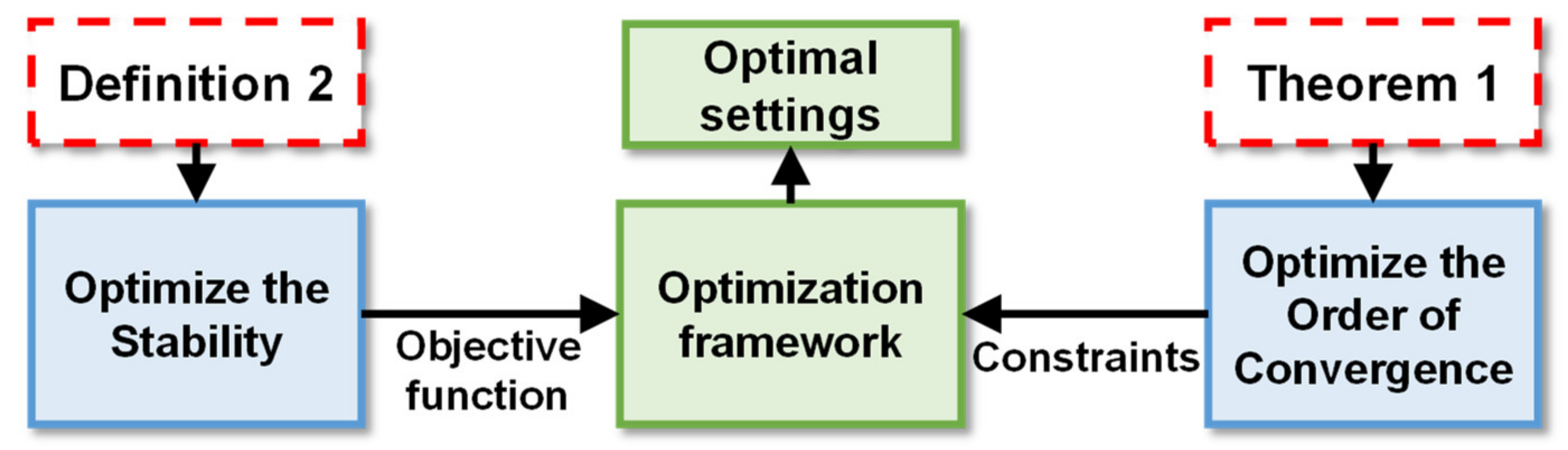
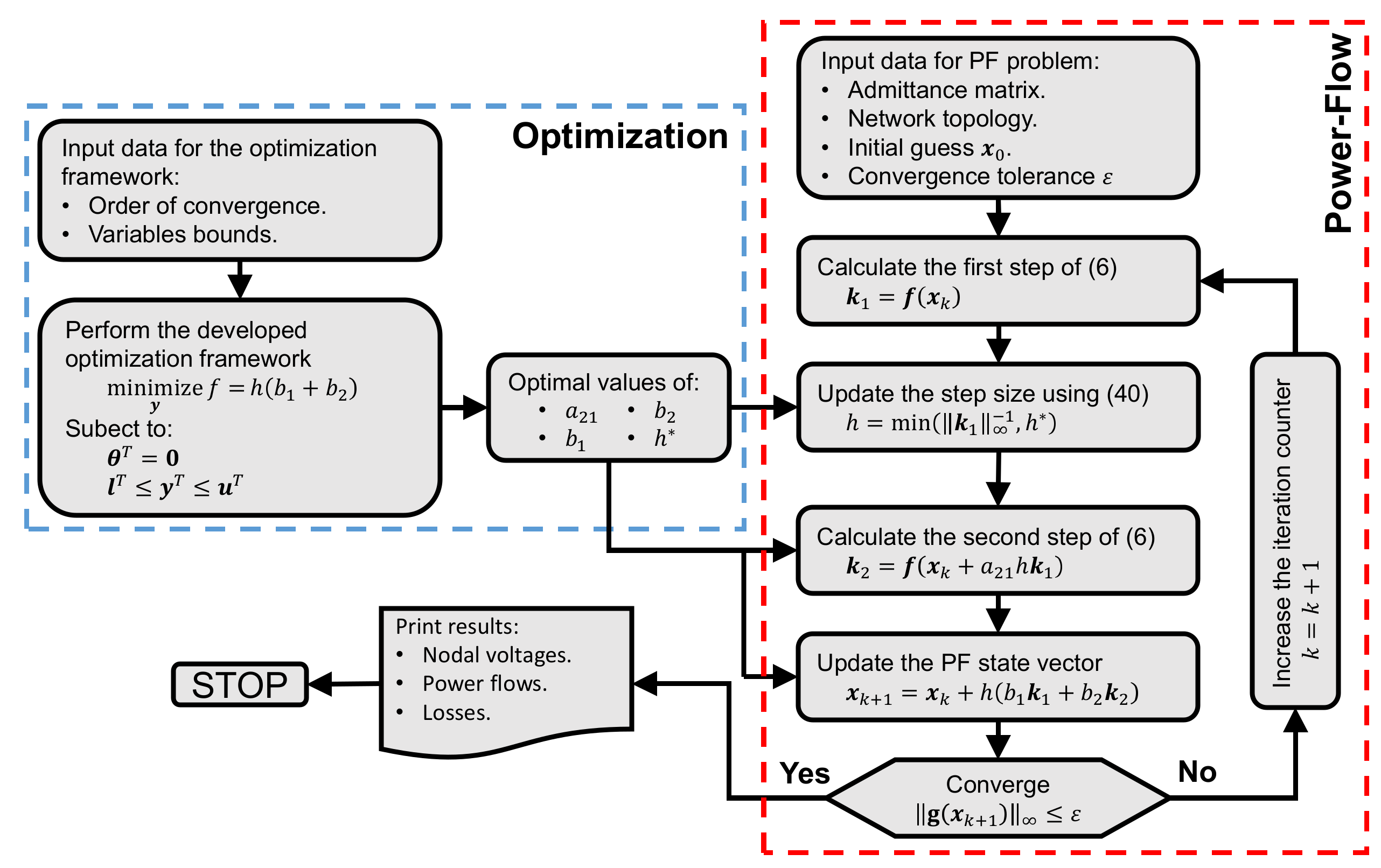
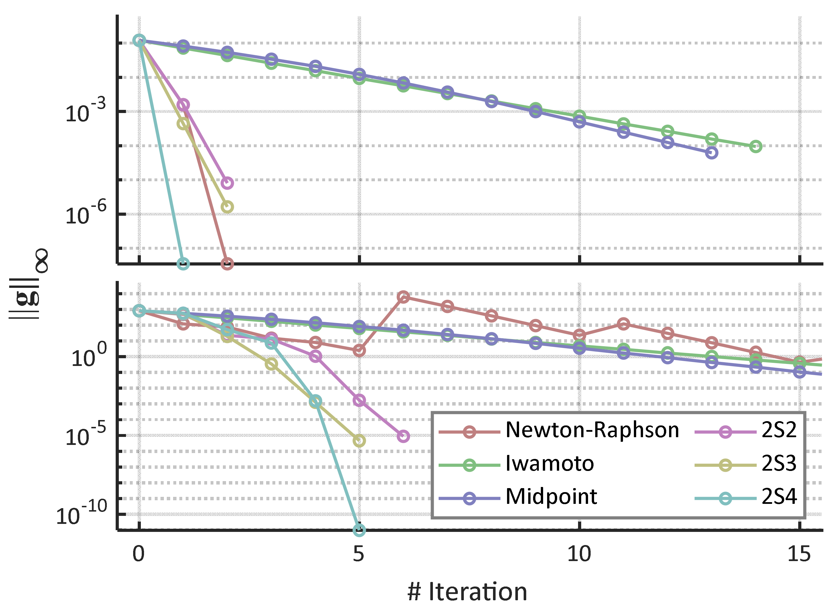
23]. As a mathematical analysis of these methods has not yet been carried out, it is not easy to know if the guidelines followed so far to develop RK-based solvers is the optimal strategy or not. This is very relevant since a proper adjustment of the parameters involved in the solution procedure might boost the numerical stability, convergence rate, and efficiency of the RK-based techniques. In this sense, this paper develops an optimization framework by which the different parameters involved in the iterative algorithm of the RK-based approaches are optimally tuned to maximize the order of convergence and numerical stability. To this end, various theorems are derived, and an optimization procedure is developed and discussed. In this sense, only minimal and acceptable heuristic assumptions were made. Based on the proposed optimization framework, three novel PF solvers with quadratic, cubic, and 4th order of convergence are developed based on the generic numerical scheme of the two-stage RK formulas. To check the adequacy of the novel proposals, various case studies are performed in several large-scale well- and ill-conditioned systems, comparing the obtained results with other benchmark solvers. This way, the present work supposes an advance with respect to others references such as [7,26], where the set of parameters that define the PF solver were tuned on the basis of heuristic criteria. In this sense, this paper aims at presenting a formal framework on the basis of theoretical foundation with the aim of acquiring the high properties of the two-stage RK-based PF solvers, thus supposing a benchmark for future contributions in the field of PF solution of ill-conditioned cases.
In the rest of this paper, Section 2 describes the PF solution using two-stage RK-based PF solvers. The proposed optimization framework for optimal setting of the parameters involved in the two-stage RK-based PF solvers is developed in Section 3. Section 4 presents three PF solvers developed by using the framework described in Section 3. Section 4 presents various numerical results obtained with the developed techniques compared with those obtained with other benchmark methods. The paper is concluded in Section 5.

2. PF Solution Using Two-Stage RK-Based Solvers

In PF problems, the nonlinear equations that relate the nodal voltages with the power injections can be posed in different forms, from the most conventional power residuals formulation to other alternative approaches, such as those based on current injections [36]. The formulation and methodologies presented in this paper can be easily adapted to most of the existing formulations. Nevertheless, the PF equations are presented based on power injections and polar form without loss of generality, as follows:
g x = g P ,   For   all   buses g Q ,   For   PQ   buses
g P i = P i s c h j = 1 n V i V j Y i j cos θ i j δ i + δ j
g Q i = Q i s c h j = 1 n V i V j Y i j sin θ i j δ i + δ j
where, g : n n denotes the set of PF equations, P i s c h and Q i s c h are the active and reactive power injected at i th bus, respectively. V i δ i is the complex voltage at i th bus. Y i j θ i j is the i j th element of the admittance matrix. In the case of polar formulation, voltage magnitudes at PQ buses along the nodal voltage angles are the unknowns. Thereby, the PF state vector is defined by:
x = δ P V , δ P Q , V P Q T
where, δ P V n g is the vector of voltage angles at PV buses, δ P Q n g is the vector of voltage angles at PQ buses and V P Q n l is the vector of voltage angles at PQ buses. On the other hand, n g and n l represent the total number of PV and PQ buses, respectively. Therefore, the size of the state vector is equal to n = 2 n l + n g . The notations of PQ and PV are widely employed in PF analysis and refer to the number of unknowns of each bus in the systems. For the sake of self-sufficiency, a brief explanation of each bus can be found below:
  • PQ buses: are normally load buses in which the voltage angle and magnitude are unknown, and the active (P) and reactive (Q) power injections are known.
  • PV buses: are normally generator buses in which the voltage angle is unknown, the active (P) power injection and the voltage angle (V) are known, and the reactive power injection is an independent variable.
  • Slack: one or various buses in the system have their voltage fixed, while the power injections are dependent variables.
The set of Equation (1) is clearly nonlinear. Although some linear approaches have been proposed (e.g., see [40]), PF problems are normally solved using nonlinear iterative routines. Among the different solvers available, NR is the most widely employed in PF calculations, which is defined by the following mapping:
x k + 1 = x k g x k 1 g x k
where · k stands for the iteration counter, g = x g n × n is the Jacobian matrix of the PF equations and · 1 : n n is the inverse operator. The heaviest calculation of the map (5) is the LU factorization of the Jacobian matrix, which has a computational cost of O n 3 . Moreover, NR has quadratic and local convergence, which means that convergence properties are lost if the initial guess (say x 0 ) is far away of the PF solution. It supposes a great barrier of NR in PF solution of ill-conditioned cases. A formal definition of PF ill-conditioned cases was given in Definition 1.
According to Definition 1, NR would diverge in ill-conditioned cases if a flat start is used. To overcome the issues of NR and other solvers in such cases, some authors have developed robust PF solvers by years (see Literature Review). In particular, the two-stage RK-based methods, which are a special application of the Continuous Newton’s principle [7], are carried out as follows:
k 1 = f x k   k 2 = f x k + a 21 h k 1   x k + 1 = x k + h b 1 k 1 + b 2 k 2
where f = g x 1 g x ; h is the step size; and a 21 , b ’s are parameters that define the method. As an example, for the PF solver based on the Midpoint rule (MP) developed in [26], a 21 = 1 2 , b 1 = 0 and b 2 = 1 . The step size has to be initialized and it is typically adapted using heuristic rules [7,25]. This way, the parameters involved (6) have been traditionally determined based on either standard formulations [23] or heuristic foundations, without analysing the mathematical features of the mapping (6) in detail. This is addressed in the following section.
It is worth noting that (6) requires two LU factorizations each iteration, which entails almost doubling the computational cost of NR. Nevertheless, it has been empirically proved that (6) is more widely convergent than NR and therefore more suitable for ill-conditioned cases.

3. Optimal Settings for Two-Stage RK-Based PF Solvers

The numerical scheme (6) has four degrees of freedom, namely a 21 , b 1 , b 2 , and h . In this paper, an optimization framework is developed for setting these parameters, thus maximizing its convergence rate and numerical stability. In this regard, it is suitable to introduce Theorem 1 and Definition 2.
Theorem 1. 
([41]). Let F 1 x and  F 2 x be fixed point functions of the nonlinear equation  g x = 0 . Let the iterative methods defined by  x k + 1 = F 1 x k and x k + 1 = F 2 x k be of order p 1 and  p 2 , respectively. Then, the convergence order of the iterative method corresponding to the fixed-point function  F = F 1 F 2 x is  p 1 × p 2 .
Definition 2 
([42]). A fixed point  x * of a map  F   : C n n is hyperbolic if the Jacobian of the equation  F ˙ = F x x at  x * has no eigenvalues with a zero real part. In addition,  x * is asymptotically stable if all the eigenvalues of F ˙ at  x * have a modulus  1 . A hyperbolic point can be:
  • Sink: if all the eigenvalues of the Jacobian of  F ˙ have a negative real part.
  • Source: if all the eigenvalues of the Jacobian of  F ˙ have a positive real part.
To ensure the numerical stability of iterative mappings such as (5) and (6), PF solutions (namely x * such that g x * ) should be asymptotically stable [7]. The following sections derive the order of convergence and numerical stability of the mapping (6), to finally establish an optimization framework for tuning the degrees of freedom of this numerical scheme, thus maximizing its numerical properties.

3.1. Order of Convergence

On the basis of Theorem 1, the mapping (6) may achieve up to 4th order of convergence, since actually two Newton iterations with quadratic convergence are nested. However, as seen in the results reported in [26], the two-stage RK-based solvers studied so far present a clear linear convergence rate. Therefore, it is relevant to pose the following question: under which conditions would the mapping (6) achieve 4th order of convergence? To respond to this question, the order of convergence of the mapping (6) is derived below, for which the Taylor Expansion technique has been used (e.g., see [43]).
Firstly, the Taylor expansions of g and g about x * as follows:
g x g x * e + C 2 e 2 + C 3 e 3 + O e 4
g x g x * I + 2 C 2 e + 3 C 3 e 2 + O e 3
where e = x x * n , e i = e , e , , e i times , C j = 1 / j ! g r 1 g j r L i n , n , g j L n × × n , n , g r 1 L n and I n × n is the identity matrix. Now, let us assume that:
g x 1 = c 1 I + c 2 e + c 3 e 2 g x * 1 + O e 3
where c ’s are coefficients. The following inverse definition can be deduced:
g x 1 g x = g x g x 1 = I
Solving the resulting linear system, one obtains:
g x 1 = I 2 C 2 e + 4 C 2 2 3 C 3 e 2 g x * 1 + O e 3
At this point, k 1 can be developed, as follows:
k 1 = g x 1 g x = 2 C 3 2 C 2 2 e 3 + C 2 e 2 e + O e 4
The following expression can be extracted by developing the second step in (6):
e 1 = x + a 21 h k 1 x * = 2 a 21 h C 3 2 a 21 h C 2 2 e 3 + a 21 h C 2 e 2 + 1 a 21 h e + O e 4
For the second stage of (6), the Taylor series expansion of g x + a 21 h k 1 and g x + a 21 h k 1 about x * are needed, which are given by:
g x + a 21 h k 1 g x * 1 a 21 h e + a 21 2 h 2 a 21 h + 1 C 2 e 2 + 3 a 21 2 h 2 a 21 3 h 3 a 21 h + 1 C 3 2 a 21 2 h 2 C 2 2 e 3 + O e 4
g x + a 21 h k 1 g x * I + 2 a 21 2 h 2 4 a 21 h + 2 C 2 e 2 + O e 3
While inversion of (15) yields:
g x + a 21 h k 1 1 = I + 2 a 21 h 2 C 2 e + 4 a 21 2 h 2 10 a 21 h + 4 C 2 2 + 6 a 21 h 3 a 21 2 h 2 3 C 3 e 2 g x * 1 + O e 3
Now, k 2 can be developed:
k 2 = g x + a 21 h k 1 1 g x + a 21 h k 1 = a 21 2 h 2 3 a 21 h + 1 C 2 e 2 + a 21 h 1 e + O e 3
Finally, the error vector at k + 1 is given by:
e k + 1 = x k + h b 1 k 1 + b 2 k 2 x * = θ 4 e k 3 + θ 3 e k 2 + θ 2 e k + O e k 4
where
θ 2 = a 21 b 2 h 2 h b 1 + b 2 + 1
θ 3 = a 21 2 b 2 h 2 3 a 21 b 2 h + b 1 + b 2 h C 2
θ 4 = 6 a 21 2 b 2 h 2 2 a 21 3 b 2 h 3 8 a 21 b 2 h + 2 b 1 + b 2 h C 3 + 2 a 21 3 b 2 h 3 8 a 21 2 b 2 h 2 + 10 a 21 b 2 h 2 b 1 + b 2 h C 2 2
The expression (18) indicates the order of convergence of the mapping (6). From this equation, the following conclusions can be extracted:
  • The mapping (6) achieves 4th order of convergence if θ 2 = θ 3 = θ 4 = 0 ;
  • The mapping (6) achieves 3rd order of convergence if θ 2 = θ 3 = 0 ;
  • The mapping (6) achieves 2nd order of convergence if θ 2 = 0 ;
  • Convergence rate of (6) is linear if θ 2 0 .
Therefore, the development above establishes the condition by which the mapping (6) achieves high order of convergence. To do this, the different parameters must be tuned so that the conditions a–d are met. Since the mapping (6) presents four degrees of freedom, all these conditions can be met without any problem.

3.2. Numerical Stability

The numerical stability of an iterative map can be deduced on the basis of the Definition 2, from which it is deduced that the fixed points of the algorithm should be asymptotically stable. To derive the stability of the mapping (6), let us define the differential equation associated, as follows:
F ˙ = h b 1 k 1 + b 2 k 2
By differentiating (22) with respect to x , one obtains:
x F ˙ = h b 1 x k 1 + b 2 x k 2
Respectively, the following expressions can be derived:
x k 1 = x f x = x g x 1 g x g x 1 g x
x k 2 = x f x + a 21 h k 1 = x g x + a 21 h k 1 1 g x + a 21 h k 1 g x + a 21 h k 1 1 g x + a 21 h k 1
Evaluating (23)–(25) and k 1 at equilibrium point x * , one obtains:
x k 1 x * = I
k 1 x * = x *
x k 2 x * = I
x F ˙ x * = h b 1 + b 2 I
From (26)–(29), the numerical stability of (6) can be deduced. Indeed, to ensure that x * is asymptotically stable, the following inequality must hold:
0 h b 1 + b 2 1
As observed, inequality (30) can be ensured by simply manipulating the value of h , b 1 , and b 2 .

3.3. Optimal Setting for Parameters

The mathematical deductions developed in previous sections establish the necessary conditions for maximizing the order of convergence and numerical stability of the mapping (6). As observed, conditions a–d and inequality (30) can be met by properly setting the values of a 21 , b 1 , b 2 , and h . This deduction allows us to establish an optimization problem to calculate the optimal values of these parameters. Consequently, Equation (30) can be established as the objective function of a minimization problem. On the other hand, the conditions a–b can be introduced as constraints, so that different parameters can be tuned to achieve a determined order of convergence. This idea is sketched in Figure 1.
It is worth noting that a 21 cannot be nullified, otherwise x * may not be a fixed point of (6). Taking into account this premise and the ideas commented above, the following optimization problem can be established:
minimize y   f = h b 1 + b 2
subject   to :
θ T = 0
l T y T u T
where
y = a 21 ,   b 1 ,   b 2 , h T
θ = θ 2 ,   f o r   q u a d r a t i c   c o n v e r g e n c e   r a t e
θ = θ 2 , θ 3 T ,   f o r   c u b i c   c o n v e r g e n c e   r a t e
θ = θ 2 , θ 3 , θ 4 T ,   f o r   4 t h   o r d e r   o f   c o n v e r g e n c e
l = 1 / 3 , 1 / 3 , 1 / 3 , 0.1 T
u = 1 , 2 , 2 , 2 T
As seen, the problem (31) aims at minimizing (30) with the objective of improving the numerical stability of (6), taking the parameters involved in (6) as the variables of the problem (see (34)). On the other hand, constraints (32) establish the necessary conditions for achieving a determined order of convergence. This way, (32) should be equal to (35) to achieve quadratic convergence, equal to (36) to make the mapping (6) cubic convergent and finally equal to (37) for achieving 4th order of convergence. Finally, (38) and (39) establish upper and lower bounds on the variables, whose values have been established from empirical evidence.
The optimization problem (31)–(33) may be nonconvex; nevertheless, it is usually easily solvable using conventional solvers such as Gurobi [44], which can be acquired under free license programs for academic and research purposes. In addition, the proposed optimization paradigm is very small-scale (the vector of variables has just four elements), and thus is manageable for average machines.
Using the optimization framework explained above, three novel PF solvers have been developed based on (6) with quadratic, cubic, and 4th order of convergence, whose parameter settings are reported in Table 1 (in this table, h * indicates the optimal value of the step size while f * stands for the value of the objective function (31) for the calculated optimal settings). In this table, the value of the objective function is also reported. As observed, the higher the order of convergence, the higher the objective function, which is logical since more constraints are actually imposed on θ . From this result it is deduced that the mapping (6) turns weaker as the order of convergence grows, which is in consonance with the conclusions extracted for other HONL solvers [8].

3.4. A Rule for Updating the Step Size

It is worth noting that, according to the procedure described in (23)–(30), the value of the objective function reported in Table 1 is only obtained at the equilibrium point x * . Thus, during the rest of the iterative process, stability of mapping (6) is actually guided by (23). In this case, eigenvalues of (23) are proportional to both k 1 and k 2 , or more concisely proportional to g x . A direct consequence of this is that h * (see Table 1), should not be taken at the beginning of the iterative process, when large mismatches are expected. Instead, h may be fixed shorter in order to counteract the effect of g x , and then progressively increased up to its optimal value. Ideally, h should be inversely proportional to k 1 + k 2 . However, it is necessary to calculate the value of h prior to calculating k 2 . Therefore, the latter cannot be used to update the step size. Nevertheless, it is reasonable to think that the whole mapping will be stable if the first step in (6) is stable as well. Therefore, the step size could be updated only using the value of k 1 . Keeping this in mind, the following updating rule is proposed:
h = min k 1 1 , h *
As seen, the rule (36) meets the premises exposed above. Indeed, the step size would be short at first iterations, when the mismatch is expected to be high. In such a case, the step size would be equal to the minimum value in (40), which presumably would be k 1 1 . As seen in (23), the stability of the mapping is guided by the value of k 1 ; more precisely, the larger value of k 1 , the less robust the map is. By these reasons, the inverse of the infinity norm of k 1 has been taken in (40) to update the step size. In contrast, one the algorithm successfully evolves, one is keen to enlarge the step size as much as possible to achieve high convergence rate. In such a case, the rule (40) would impose the optimal value of the step size h * . It is worth noting that, unlike other updating rules proposed in the literature (e.g., see [25]), it is based on theoretical findings. This section is finalized with Figure 2, where the proposed flowchart for PF calculation is shown using the mapping (6) with optimal settings. In this case, ε + has been established as the convergence threshold.

4. Numerical Experiments

This section presents various numerical results with the aim of checking the performance of the developed solvers and validating the proposed optimization framework. Due to this paper being focused on realistic cases, the following large-scale networks have been considered:
  • The 3012-bus snapshot of the Polish transmission system at 2007–2008 evening peak [45].
  • The 6243-bus system formed by combining the 3374-bus snapshot of the Polish transmission system at 2007–2008 evening peak [45] and the 2869-bus portion of the European transmission system [46,47]. The data of this system is available in [48].
  • The 12,110-bus system formed by combining the 2869-bus and 9241-bus portions of the European transmission system [46,47]. The data of this system is available in [48].
The main characteristics of the considered systems are collected in Table 2. In this table, the condition number refers to the index usually used to measure the degree of ill-conditioning of a PF case [26], so that the larger condition number, the higher degree of ill-conditioning. Typically, the condition number can be calculated as follows:
C N = g x F g x 1 F
where, F : n + , stands for the Frobenius norm. Comparing the condition number of the studied systems with those reported in [15], it seems clear that the considered systems are naturally ill-conditioned and therefore suitable for the present study. As seen, they are based on real networks and are clearly large-scale. In addition, their condition numbers are high, which denotes ill-conditioning character [26]. In order to check the performance of the developed PF solvers and validate them, they have been compared with the following benchmark techniques:
  • The conventional NR in polar coordinates and power mismatches.
  • The Iwamoto’s method in polar coordinates and power mismatches [20].
  • The PF solver based on the MP rule developed in [26], for which the guidelines provided in the references for its computational implementation have been followed.
While NR is by far the most widely used PF solver, the Iwamoto’s technique has been considered as a benchmark robust technique in multiple related references (e.g., see [7], [25]). On the other hand, MP is a solver based on the two-stage RK scheme (6), which offered acceptable results in [26]. In this way, it can be considered as a good comparing technique for validating the developed optimization framework and showing how the numerical mapping (6) can achieve superior features by properly tuning the parameters involved.
All the tested methods have been coded under a Matlab R2019a environment, using the software package Matpower v7.0 [49]. This software is open source, thus allowing us to easily code the different tested methodologies. Moreover, the considered systems are available in its library of problems. In all simulations, the convergence threshold has been set as equal to 10 4 .

4.1. Convergence Rates for Base Cases

Firstly, the iteration number of the tested solvers is compared in Table 3. The considered solvers have been compared in two situations. On the one hand, the default starting point provided in Matpower is used for initializing the iterative procedures. This initial guess is considered a better approximation than the flat start, as shown in [50]. On the other hand, the conventional flat start takes all the voltage angles equal to 0 rad and the voltage magnitudes at PQ buses equal to 1 pu. As seen in Table 3, all the considered solvers converged from the default point, while NR diverged from a flat start, which indicates that the studied networks are actually ill-conditioned cases. In all cases, the developed solvers with optimal settings outperformed the Iwamoto’s method and MP. By comparing the results reported with those obtained with MP, it can be deduced that the mapping (6) can achieve superior convergence features if the parameters involved are optimally tuning. This evidence validates the merits of the developed optimization framework, which allows us to achieve the best performance of the numerical scheme (6). In comparison with NR, 2S2 converged in all cases employing the same number of iterations, while 2S3 and 2S4 required less iterations. This result is logical since while 2S2 presents a quadratic convergence rate, the other developed techniques have superior convergence orders.
To get a better overview, Figure 3 plots the convergence curves for the 3012-bus systems from the default and flat starters. In this figure, the superior convergence properties of 2S3 and 2S4 are clearly appreciated. Indeed, these solvers attained lower residuals than NR, while the convergence profiles for 2S2 and NR were similar. It is worth noting that the convergence features of the Iwamoto’s method and MP are clearly linear. As commented, this drawback contributes to the low computational degree of most of robust methods. When a flat start is considered, NR failed as it oscillates for a large number of iterations. For the rest of the solvers, convergence features are normally degraded because the flat start is further away from the solution [50]. Even so, the developed solvers still presented good convergence properties, and converged in an acceptable number of iterations.

4.2. Convergence Rates with Reactive Limits

In power system analysis, the operation of some components is subjected to functional limits. One clear example is the reactive limits of generators. It is fundamental to consider this aspect in PF analysis [51]. As with other methodologies (e.g., see [7]), these restrictions are not directly considered, however, they can be incorporated through simple PV-PQ switching methodologies [50]. One simple procedure was described in [50] and is sketched in Figure 4. Basically, the PF is initially solved without considering any reactive bound. If the PF solution is attained, the algorithm checks if any limit has been violated. In affirmative cases, the PV buses in which some limit has been hit are converted to PQ, taking the surpassed threshold as the power injection of the new bus. Then, the PF problem is sequentially repeated until a feasible solution is achieved or there are no longer PV buses, in which case the problem is declared unfeasible. This methodology presents two great challenges for PF solvers:
  • Each time the PF problem is run, the size of the system is increased because more PQ buses (which contribute with two variables and two equations) are incorporated to the system.
  • As the size of the system grows and more PQ buses are added, the ill-conditioned issues are more notable. To overcome this problem, the algorithm detailed in Figure 4 takes the solution of the previous PF procedure as the initial guess for the following process, since this approach will intuitively be a better initialization than the flat start.
The strategy described above has been selected for this paper because it can be incorporated into the considered solvers without any problem. Table 4 reports the total number of iterations in the presence of reactive limits at PV buses. As seen, more iterations are typically needed to achieve a feasible solution, which is logical since normally various PF problems must be sequentially solved. As expected, NR failed in all cases from a flat start while the remainder of solvers successfully converged in all cases. Clearly, the developed approaches notably outperformed the other robust methods considered. Nevertheless, NR occasionally outperformed 2S2 from a default starter, requiring one or two fewer iterations to converge. 2S3 normally employed less iterations than NR, with the exception of the 3012-bus system, in which the developed solver required one more iteration. On the other hand, 2S4 outperformed NR in all cases. These results are explained by the influence of the step size, and as can be seen in Figure 5, it does not achieve its optimal value (and therefore the maximum order of convergence) after various iterations.

4.3. Influence of the Loading Level

It has been well reported that the loading level may degrade the convergence properties of PF solvers [8,25]. This section is devoted to analyzing how the loading level affects the performance of the developed solvers. In this case, the loading profile of the studied systems has been increased by multiplying the active power injections in all buses and the reactive power injections at PQ buses by a real positive parameter called loading level [51]. Figure 6 plots the total number of iterations required by the developed solvers to converge in the 3012-bus system from a flat start with different loading levels. As expected, the developed solvers usually took more iterations for converging with high loading conditions. As observed, 2S4 normally outperformed the other developed techniques, which was expected because this method has the highest convergence order.
As observed in Figure 6, the highest loading level had the greatest number of iterations required to converge. This result is aligned with the conclusions drawn in other references [52]. It is pointed out that most PF solvers suffer from slow convergence in the vicinity of the maximum loadability point. This situation is illustrated in Figure 7, where the convergence profile in the 3012-bus system using 2S2 from a flat start is compared for two scenarios: baseload conditions and the maximum loading level of this system (1.2734 pu). As observed, convergence properties of the method are notably degraded with heavy loading conditions, converging linearly to the solution.
As the maximum loading level supposes the most demanding conditions, it is relevant to compare the studied solvers in such a scenario. In this regard, Table 5 reports the total number of iterations of the different compared techniques for the maximum loading level of each system. As expected, all the techniques required more iterations to converge compared with the base case. The developed solvers were, in general, well-behaved, outperforming the other robust methodologies. Compared to NR, which diverged in all cases from a flat start, the new proposals were competitive. Indeed, 2S2 required the same number of iterations, while 2S3 and 2S4 were able to improve the results obtained with NR from the default starter, requiring up to three fewer iterations.

4.4. Computational Cost

One of the many barriers to the wide application of the existing robust PF approaches is their high computational complexity, making them impractical for some applications such as security analysis [53]. In this regard, it is necessary to compare the total computational time required by the developed techniques and the other robust solvers. Table 6 reports the computation time (in milliseconds) consumed by the studied solvers for the base cases. These results were obtained on a 3.4 GHz Intel Core i7-8750H CPU 2.2 GHz personal laptop (16.00 GB RAM). As observed, although NR was normally the most efficient solver, the results obtained with the developed methods are in the same order, especially in the case of 2S4, without this representing a significant barrier to its implantation in industry tools. More relevant is the comparison of the developed methods with the results obtained with the other robust approaches. When starting from the default point, NR was occasionally more efficient than 2S2, which is expected since this solver presents quadratic convergence, similarly to NR, but involves more operations. Likewise, 2S3 was slower than NR from a default point since, in this case, its third order of convergence was not enough to compensate for the extra calculations in comparison with NR. In contrast, 2S4. However, it is noteworthy that the developed methods were the winner from a flat starter. In this regard, ill-conditioned cases are defined from a flat starting point. Considering that the developed methods are focused on these particular cases, it can be concluded that the studied solvers outperformed other robust techniques in ill-conditioned cases.
In light of the results above, it seems clear that NR is still preferred in well-conditioned cases. Nevertheless, considering that NR would fail in ill-conditioned cases, the developed solvers can be considered more universal because of their good overall performance in both well and ill-conditioned cases. In this sense, as observed in Table 6, their superiority with respect to other robust solvers was notable. Unlike the robust benchmark techniques, the studied methods were still competitive in well-conditioned methods, implying only a marginal extra computational burden compared to NR, which justifies their use in a wide variety of PF cases.
The computational cost of a PF solver is mainly determined by the total LU factorizations computed to converge [7]. In this sense, although the developed solvers require two LU factorizations per iteration, their higher convergence order make them computationally competitive, even with NR. Thus, when NR computed the same or less LU factorizations than the developed methods, it was the winner. At this point, it is worth noting that NR requires one LU decomposition per iteration, while the developed solvers need two. However, as the developed methods present higher convergence order, they usually need less iterations to converge and therefore less LU decompositions in total, which explains why the developed methods were computationally more efficient than NR in most of cases and much more efficient than other robust solvers used in the comparison. Indeed, as seen in Figure 8, the developed methods normally needed to compute few LU factorizations, even equalling the total computational cost of NR. This is the reason why MP is very inefficient. Indeed, although this technique also computes two LU factorizations per iteration, its convergence rate is linear, usually employing more iterations than the developed methods. This result evidences the importance of optimizing the convergence rate of iterative schemes, thus highlighting the importance of the developed optimization framework in making the developed solvers practical and attractive.

5. Conclusions and Future Works

This paper has presented an optimization methodology for optimally tuning the parameters involved in two-stage RK-based PF solvers. Traditionally, these parameters have been tuned, attending to the standard structure of RK formulas, without checking if this approach allows for extracting the best numerical properties of the iterative mapping. The developed optimization framework allows for the calculation of the optimal value of these parameters so that the convergence order and stability of the iterative mapping are maximized, assuming only some heuristic criteria.
Three PF solvers with quadratic, cubic, and 4th order of convergence have been developed using the proposed optimization technique. They have been tested in various large-scale, realistic, ill-conditioned systems under various demanding scenarios. Their performance has been compared with other robust approaches and NR. The robustness of the developed methods has been validated, successfully converging in all the studied systems. In addition, the new proposals were computationally competitive, even with NR, presenting acceptable computational times that make them suitable for industrial applications. The results obtained have evidenced the importance of properly tuning the parameters involved in RK-based solvers.
Future works should be focused on applying similar procedures to other PF solvers based on the Continuous Newton’s method, such as those developed in [24,25,26]. The authors expect promising results with these other techniques.

Author Contributions

Conceptualization, M.T.-V. and S.K.; methodology, M.T.-V. and S.K.; software, T.A. and S.K.; validation, M.T.-V., S.K. and T.A.; formal analysis, T.A., H.A., S.K. and F.J.; investigation, M.T.-V. and S.K.; resources, T.A., H.A. and F.J.; data curation, S.K.; writing—original draft preparation, M.T.-V. and S.K.; writing—review and editing, T.A. and F.J.; visualization, T.A. and F.J.; supervision, F.J.; project administration, F.J.; funding acquisition, T.A. and H.A. All authors have read and agreed to the published version of the manuscript.

Funding

Deanship of Scientific Research, Qassim University.

Acknowledgments

The researchers would like to thank the Deanship of Scientific Research, Qassim University for funding the publication of this project.

Conflicts of Interest

The authors declare no conflict of interest.

References

  1. Tang, K.; Dong, S.; Shen, J.; Zhu, C.; Song, Y. A Robust and Efficient Two-Stage Algorithm for Power Flow Calculation of Large-Scale Systems. IEEE Trans. Power Syst. 2019, 34, 5012–5022. [Google Scholar] [CrossRef]
  2. Sobhy, M.A.; Abdelaziz, A.Y.; Hasanien, H.M.; Ezzat, M. Marine predators algorithm for load frequency control of modern interconnected power systems including renewable energy sources and energy storage units. Ain Shams Eng. J. 2021, 12, 3843–3857. [Google Scholar] [CrossRef]
  3. Xie, N.; Torelli, F.; Bompard, E.; Vaccaro, A. Dynamic computing paradigm for comprehensive power flow analysis. IET Gener. Transm. Distrib. 2013, 7, 832–842. [Google Scholar] [CrossRef]
  4. Pourbagher, R.; Derakhshandeh, S.Y. A powerful method for solving the power flow problem in the ill-conditioned systems. Int. J. Electr. Power Energy Syst. 2018, 94, 88–96. [Google Scholar] [CrossRef]
  5. Zhao, T.Q.; Chiang, H.-N.; Koyanagi, K. Convergence analysis of implicit Z-bus power flow method for general distribution networks with distributed generators. IET Gener. Transm. Distrib. 2016, 10, 412–420. [Google Scholar] [CrossRef]
  6. Milano, F. Power System Modelling and Scripting; Springer: Berlin/Heidelberg, Germany, 2010. [Google Scholar]
  7. Milano, F. Continuous Newton’s Method for Power Flow Analysis. IEEE Trans. Power Syst. 2009, 24, 50–57. [Google Scholar] [CrossRef]
  8. Tostado-Véliz, M.; Kamel, S.; Jurado, F.; Ruiz-Rodriguez, F.J. On the Applicability of Two Families of Cubic Techniques for Power Flow Analysis. Energies 2021, 14, 4108. [Google Scholar] [CrossRef]
  9. Tinney, W.F.; Hart, C.E. Power Flow Solution by Newton’s Method. IEEE Trans. Power Appar. Syst. 1967, PAS-86, 1449–1460. [Google Scholar] [CrossRef]
  10. Sachdev, M.S.; Medicherla, T.K.P. A second order load flow technique. IEEE Trans. Power Appar. Syst. 1977, 96, 189–197. [Google Scholar] [CrossRef]
  11. Iwamoto, S.; Tamura, Y. A Fast Load Flow Method Retaining Nonlinearity. IEEE Trans. Power Appar. Syst. 1978, PAS-97, 1586–1599. [Google Scholar] [CrossRef]
  12. Stott, B.; Alsac, O. Fast Decoupled Load Flow. IEEE Trans. Power Appar. Syst. 1974, PAS-93, 859–869. [Google Scholar] [CrossRef]
  13. Idema, R.; Lahaye, D.J.P. Computational Methods in Power System Analysis; Schilders, W., Ed.; Atlantis Press: Paris, France, 2014. [Google Scholar]
  14. Tinney, W.F.; Walker, J.W. Direct solutions of sparse network equations by optimally ordered triangular factorization. Proc. IEEE 1967, 55, 1801–1809. [Google Scholar] [CrossRef] [Green Version]
  15. Derakhshandeh, S.Y.; Pourbagher, R.; Kargar, A. A novel fuzzy logic Levenberg-Marquardt method to solve the ill-conditioned power flow problem. Int. J. Electr. Power Energy Syst. 2018, 99, 299–308. [Google Scholar] [CrossRef]
  16. Tortelli, O.L.; Lourenco, E.M.; Garcia, A.V.; Pal, B.C. Fast Decoupled Power Flow to Emerging Distribution Systems via Complex pu Normalization. IEEE Trans. Power Syst. 2015, 30, 1351–1358. [Google Scholar] [CrossRef]
  17. Li, X.; Li, F.; Yuan, H.; Cui, H.; Hu, Q. GPU-Based Fast Decoupled Power Flow with Preconditioned Iterative Solver and Inexact Newton Method. IEEE Trans. Power Syst. 2017, 32, 2695–2703. [Google Scholar] [CrossRef]
  18. Milano, F. Implicit Continuous Newton Method for Power Flow Analysis. IEEE Trans. Power Syst. 2019, 34, 3309–3311. [Google Scholar] [CrossRef]
  19. Iwamoto, S.; Tamura, Y. A Load Flow Calculation Method for Ill-Conditioned Power Systems. IEEE Trans. Power Appar. Syst. 1981, PAS-100, 1736–1743. [Google Scholar] [CrossRef]
  20. Tate, J.E.; Overbye, T.J. A Comparison of the Optimal Multiplier in Polar and Rectangular Coordinates. IEEE Trans. Power Syst. 2005, 20, 1667–1674. [Google Scholar] [CrossRef]
  21. Mokhlis, H.; Shahriari, A.; Bakar, A.H.A.; Illias, H.A.; Karimi, M. Improved Step Size Newton Raphson Method using quadratic equations properties in ill-conditioned power system. Int. Trans. Electr. Energy Syst. 2014, 24, 1323–1342. [Google Scholar] [CrossRef]
  22. Shahriari, A.; Mokhlis, H.; Karimi, M.; Bakar, A.H.A.; Illias, H.A. Quadratic Discriminant Index for Optimal Multiplier Load Flow Method in ill conditioned system. Int. J. Electr. Power Energy Syst. 2014, 60, 378–388. [Google Scholar] [CrossRef]
  23. Butcher, J.C. Numerical Methods for Ordinary Differential Equations, 2nd ed.; Wiley: Chichester, UK, 2008. [Google Scholar]
  24. Tostado-Véliz, M.; Kamel, S.; Jurado, F. Development of different load flow methods for solving large-scale ill-conditioned systems. Int. Trans. Electr. Energy Syst. 2019, 29, e2784. [Google Scholar] [CrossRef]
  25. Tostado-Veliz, M.; Kamel, S.; Jurado, F. A Robust Power Flow Algorithm Based on Bulirsch-Stoer Method. IEEE Trans. Power Syst. 2019, 34, 3081–3089. [Google Scholar] [CrossRef]
  26. Tostado-Véliz, M.; Kamel, S.; Jurado, F. Comparison of various robust and efficient load-flow techniques based on Runge-Kutta formulas. Electr. Power Syst. Res. 2019, 174, 105881. [Google Scholar] [CrossRef]
  27. Xie, N.; Bompard, E.; Napoli, R.; Torelli, F. Widely convergent method for finding solutions of simultaneous nonlinear equations. Electr. Power Syst. Res. 2012, 83, 9–18. [Google Scholar] [CrossRef]
  28. Torelli, F.; Vaccaro, A. A second order dynamic power flow model. Electr. Power Syst. Res. 2015, 126, 12–20. [Google Scholar] [CrossRef]
  29. Torelli, F.; Vaccaro, A.; Pepiciello, A. A Dynamic Framework for Multiobjective Mixed-Integer Optimal Power Flow Analyses. Technol. Econ. Smart Grids Sustain. Energy 2021, 6, 14. [Google Scholar] [CrossRef]
  30. Gnanambal, K.; Marimuthu, N.S.; Babulal, C.K. Three-phase power flow analysis in sequence component frame using Hybrid Particle Swarm Optimization. Appl. Soft Comput. 2011, 11, 1727–1734. [Google Scholar] [CrossRef]
  31. Davoodi, E.; Hagh, M.T.; Zadeh, S.G. A hybrid Improved Quantum-behaved Particle Swarm Optimization–Simplex method (IQPSOS) to solve power system load flow problems. Appl. Soft Comput. 2014, 21, 171–179. [Google Scholar] [CrossRef]
  32. Derakhshandeh, S.Y.; Pourbagher, R. Application of high-order Newton-like methods to solve power flow equations. IET Gener. Transm. Distrib. 2016, 10, 1853–1859. [Google Scholar] [CrossRef]
  33. Tostado, M.; Kamel, S.; Jurado, F. Developed Newton-Raphson based Predictor-Corrector load flow approach with high convergence rate. Int. J. Electr. Power Energy Syst. 2019, 105, 785–792. [Google Scholar] [CrossRef]
  34. Tostado-Veliz, M.; Kamel, S.; Jurado, F. Two Efficient and Reliable Power-Flow Methods with Seventh Order of Convergence. IEEE Syst. J. 2021, 15, 1026–1035. [Google Scholar] [CrossRef]
  35. Alharbi, T.; Tostado-Véliz, M.; Alrumayh, O.; Jurado, F. On Various High-Order Newton-Like Power Flow Methods for Well and Ill-Conditioned Cases. Mathematics 2021, 9, 2019. [Google Scholar] [CrossRef]
  36. Alam, M.J.E.; Muttaqi, K.M.; Sutanto, D. A Three-Phase Power Flow Approach for Integrated 3-Wire MV and 4-Wire Multigrounded LV Networks with Rooftop Solar PV. IEEE Trans. Power Syst. 2013, 28, 1728–1737. [Google Scholar] [CrossRef]
  37. Saleh, S.A. The Formulation of a Power Flow Using dq Reference Frame Components—Part I: Balanced 3ϕ Systems. IEEE Trans. Ind. Appl. 2016, 52, 3682–3693. [Google Scholar] [CrossRef]
  38. Pires, R.; Mili, L.; Chagas, G. Robust complex-valued Levenberg-Marquardt algorithm as applied to power flow analysis. Int. J. Electr. Power Energy Syst. 2019, 113, 383–392. [Google Scholar] [CrossRef]
  39. Tostado-Véliz, M.; Kamel, S.; Jurado, F. Power flow solution of Ill-conditioned systems using current injection formulation: Analysis and a novel method. Int. J. Electr. Power Energy Syst. 2021, 127, 106669. [Google Scholar] [CrossRef]
  40. Yang, J.; Zhang, N.; Kang, C.; Xia, Q. A State-Independent Linear Power Flow Model with Accurate Estimation of Voltage Magnitude. IEEE Trans. Power Syst. 2017, 32, 3607–3617. [Google Scholar] [CrossRef]
  41. Traub, J.F. Iterative Methods for the Solution of Equations; Chelsea: New York, NY, USA, 1982. [Google Scholar]
  42. Lee, J.; Chiang, H.-D. Convergent regions of the Newton homotopy method for nonlinear systems: Theory and computational applications. IEEE Trans. Circuits Syst. I Fundam. Theory Appl. 2001, 48, 51–66. [Google Scholar] [CrossRef]
  43. Cordero, A.; Torregrosa, J.R.; Triguero-Navarro, P. A General Optimal Iterative Scheme with Arbitrary Order of Convergence. Symmetry 2021, 13, 884. [Google Scholar] [CrossRef]
  44. Gurobi, the Fastest Solver. Available online: https://www.gurobi.com/ (accessed on 10 September 2021).
  45. Matpower User’s Manual. Available online: https://matpower.org/docs/manual.pdf (accessed on 10 September 2021).
  46. Josz, C.; Fliscounakis, S.; Maeght, J.; Panciatici, P. AC Power Flow Data in MATPOWER and QCQP Format: Itesla, RTE Snap-Shots, and PEGASE. 2016. Available online: https://arxiv.org/abs/1603.01533 (accessed on 10 September 2021).
  47. Fliscounakis, S.; Panciatici, P.; Capitanescu, F.; Wehenkel, L. Contingency Ranking with Respect to Overloads in Very Large Power Systems Taking into Account Uncertainty, Preventive, and Corrective Actions. IEEE Trans. Power Syst. 2013, 28, 4909–4917. [Google Scholar] [CrossRef] [Green Version]
  48. MATPOWER Ill-Conditioned Systems Used for Validating Power-Flow Techniques. Available online: https://zenodo.org/record/3514739 (accessed on 10 September 2021).
  49. Zimmerman, R.D.; Murillo-Sanchez, C.E.; Thomas, R.J. MATPOWER: Steady-State Operations, Planning, and Analysis Tools for Power Systems Research and Education. IEEE Trans. Power Syst. 2011, 26, 12–19. [Google Scholar] [CrossRef] [Green Version]
  50. Tostado-Veliz, M.; Alharbi, T.; Alrumayh, O.; Kamel, S.; Jurado, F. A Novel Power Flow Solution Paradigm for Well and Ill-Conditioned Cases. IEEE Access 2021, 9, 112425–112438. [Google Scholar] [CrossRef]
  51. Gomez-Exposito, A.; Quiles, C.G. Factorized Load Flow. IEEE Trans. Power Syst. 2013, 28, 4607–4614. [Google Scholar] [CrossRef]
  52. Pourbagher, R.; Derakhshandeh, S.Y.; Golshan, M.E.H. An adaptive multi-step Levenberg-Marquardt continuation power flow method for voltage stability assessment in the Ill-conditioned power systems. Int. J. Electr. Power Energy Syst. 2022, 134, 107425. [Google Scholar] [CrossRef]
  53. Shen, Z.; Chiang, H.-D.; Tang, Y.; Zhou, N. An online line switching methodology with look-ahead capability to alleviate power system overloads based on a three-stage strategy. Int. J. Electr. Power Energy Syst. 2020, 115, 105500. [Google Scholar] [CrossRef]
Figure 1. Sketch of the developed optimization framework for calculating the optimal settings for the parameters in (6).
Mathematics 10 01279 g001
Figure 2. Proposed flowchart for PF calculation using the mapping (6) with optimal settings.
Mathematics 10 01279 g002
Figure 3. Convergence curves for the 3012-bus systems from the default (top) and flat (bottom) initial guesses.
Mathematics 10 01279 g003
Figure 4. Auxiliary routine for considering reactive limits at PV buses.
Mathematics 10 01279 g004
Figure 5. Evolution of the step size in the 6243-bus system from a flat start using 2S2.
Mathematics 10 01279 g005
Figure 6. Total number of iterations in the 3012-bus system for different loading levels using the developed solvers from a flat start.
Mathematics 10 01279 g006
Figure 7. Convergence profile in the 3012-bus system using 2S2 from a flat start with base case conditions (continuous line) and with the maximum loading level (dashed line).
Mathematics 10 01279 g007
Figure 8. Total LU factorizations for base cases from the default starter.
Mathematics 10 01279 g008
Table 1. Optimal settings for the developed PF solvers.
Solver AcronymOrder of Convergence a 21 b 1 b 2 h * f *
2S2Quadratic11112
2S3Cubic0.651/320.701.65
2S4Fourth1/321/30.441
Table 2. Main characteristics of the studied systems.
Characteristic3012-Bus6243-Bus12,110-Bus
Buses3012624312,110
Branches3572874420,632
Generators5029891955
LoadMW27,169180,800444,791
Mvar10,20048,535102,589
Size of the state vector (n)572511,58322,264
Condition number (41) 1.56 × 10 7 7.80 × 10 7 1.20 × 10 8
Table 3. Total number of iterations for base cases.
MethodInitial Guess# Iterations
3012-Bus6243-Bus12,110-Bus
NRDefault266
IwamotoDefault142526
MPDefault132121
2S2Default266
2S3Default244
2S4Default133
NRFlatFailFailFail
IwamotoFlat323331
MPFlat262625
2S2Flat6117
2S3Flat576
2S4Flat575
Table 4. Total number of iterations with reactive limits at PV buses.
MethodInitial Guess# Iterations
3012-Bus6243-Bus12,110-Bus
NRDefault41112
IwamotoDefault407680
MPDefault366668
2S2Default51313
2S3Default51010
2S4Default366
NRFlatFailFailFail
IwamotoFlat588485
MPFlat497172
2S2Flat91814
2S3Flat81312
2S4Flat7108
Table 5. Total number of iterations with the maximum loading level.
MethodInitial Guess# Iterations
3012-Bus6243-Bus12,110-Bus
NRDefault888
IwamotoDefault272728
MPDefault202121
2S2Default888
2S3Default668
2S4Default555
NRFlatFailFailFail
IwamotoFlat323331
MPFlat262625
2S2Flat101210
2S3Flat787
2S4Flat688
Table 6. Execution times for base cases (ms).
MethodInitial GuessExecution Time
3012-Bus6243-Bus12,110-Bus
NRDefault42.12248.64540.72
IwamotoDefault298.341079.002424.24
MPDefault549.381701.423704.40
2S2Default84.52486.121058.40
2S3Default84.52324.08705.60
2S4Default42.26243.06529.20
NRFlat------
IwamotoFlat681.921424.282890.44
MPFlat1098.762106.524410.00
2S2Flat253.56891.221234.80
2S3Flat211.30567.141058.40
2S4Flat211.30567.14882.00
Publisher’s Note: MDPI stays neutral with regard to jurisdictional claims in published maps and institutional affiliations.

