On Various High-Order Newton-Like Power Flow Methods for Well and Ill-Conditioned Cases

Abstract

Recently, the high-order Newton-like methods have gained popularity for solving power flow problems due to their simplicity, versatility and, in some cases, efficiency. In this context, recent research studied the applicability of the 4th order Jarrat’s method as applied to power flow calculation (PFC). Despite the 4th order of convergence of this technique, it is not competitive with the conventional solvers due to its very high computational cost. This paper addresses this issue by proposing two efficient modifications of the 4th order Jarrat’s method, which present the fourth and sixth order of convergence. In addition, continuous versions of the new proposals and the 4th order Jarrat’s method extend their applicability to ill-conditioned cases. Extensive results in multiple realistic power networks serve to sow the performance of the developed solvers. Results obtained in both well and ill-conditioned cases are promising.

1. Introduction

Power flow calculation (PFC) supposes the most critical tool in power system analysis. It provides the initial conditions for contingency analysis or fault calculations to be an essential tool in market and planning studies [1]. In essence, PFC is stated as a non-linear problem that is customarily solved using iterative techniques.

With the growth of network size and complexity, traditional solvers are facing increasing issues on stability and computational efficiency [2]. For the sake of example, the so-called ill-conditioned systems are becoming more common [3]. In such cases, traditional solvers such as the Newton–Raphson (NR) may experience instability problems or yield inaccurate solutions [1]. These issues have motivated a recent trend on developing novel techniques for PFC, essentially devoted to either ill-conditioned cases [4,5,6,7], large-scale realistic systems [8,9], or jointly tackling both issues [2,10].

Regarding ill-conditioned cases, a huge variety of robust methods is available. The optimal multiplier-based methods were maybe the earliest robust solvers [11]. This kind of technique is quite robust and, theoretically, not divergent, which has motived their usage to provide approximate solutions of unsolvable cases [12]. However, they may be quite inefficient or trapped on local minimums, such as those reported in [4,7].

For much of the twentieth century, ill-conditioned cases were quite unusual and their analyses were almost limited to research works and academic studies. However, ill-conditioned systems are more frequently observed nowadays, which has recently motivated people to find novel schemes suitable for more complex and realistic networks. The solvers based on the continuous Newton’s method [4,6,7] are attractive for realistic systems; nevertheless, they are still relatively inefficient as various factorizations are required at each iteration. In addition, these solvers fail at turning points where the Jacobian is singular [4].

For circumventing the weaknesses of the continuous Newton-like solvers at turning points, continuation approaches [13] or Levenberg-type methods [14] have been applied. The latter has gained popularity over the continuation approaches due to its simplicity and efficiency. However, this class of techniques still presents essential issues. As reported in [14], the Levenberg-type methods may converge to nonphysical solutions. This inaccuracy is mainly due to the so-called damping factor, for which does not exist a unified tuning criterion as manifested in [2,5,10]. In addition, they are still computationally not competitive with conventional solvers.

As observed, most robust techniques are not computationally attractive. Besides the still prevalence of well-conditioned networks, this issue induces the usage of NR in industry software. However, the high-order Newton-like methods (HONL) have recently arisen as direct competitors of the conventional solvers [8,9]. The main attractiveness of HONL is their higher order of convergence, which leads them to a fast convergence, especially in stiff problems (heavy load or high R/X ratio). Additionally, these techniques are versatile enough to incorporate alternative power flow formulations such as those developed in [15]. The main limitation of HONL is their application in ill-conditioned cases, where they usually fail since they share similar robustness characteristics with the conventional NR.

In view of the above discussions, HONL seems an attractive alternative to conventional solvers; however, very few works have been conducted on studying the applicability of these methods in PFC. Motivated by the good characteristics of HONL for PFC, we have further studied the applicability of the 4th Jarrat’s method (4OJ) (the applicability of this technique for PFC was previously studied in [8]). The authors honestly believe that the main limitation of 4OJ is its very high computational cost due to the required solution of a matrix system. This issue indeed supposes a barrier for the broad application of this method in industry tools. This paper deals with this drawback by developing two novel efficient solvers with 4th and 6th order of convergence based on 4OJ. The main attraction of the introduced techniques is that they avoid the solution of the matrix system, which is replaced by much cheaper solutions of linear systems. The continuous versions of the new proposals are also presented for extending their applicability to ill-conditioned cases. The developed methods are deduced from the original structure of 4OJ; then, using the Taylor expansion technique (e.g., see [16]), the developed mappings are properly developed from achieving high convergence rates with a low computational cost. A variety of realistic cases are studied to show the performance of our proposals.

The remainder of the paper is organized as follows. Section 2 outlines the necessary background. Section 3 develops two computationally attractive modifications of 4OJ with 4th and 6th order of convergence. Section 4 presents the continuous versions of the developed methods. A simple switching strategy for incorporating the reactive limits at PV buses is presented in Section 5. Various numerical experiments with results are provided in Section 6. Section 7 discusses possible real-life applications of the developed nonlinear solvers. This paper is concluded with Section 8.

2. Background

The PF equations are stated in their most general form as a set of $n$ algebraic non-linear equations as follows:

$$g\left(\mathit{x}\right)=\mathbf{0}$$

(1)

where $g:{ℝ}^n\to {ℝ}^n$ are the power flow equations and $\mathit{x}\in {ℝ}^n$ is the vector of unknowns (state vector). The set of Equation (1) may be formulated in polar or rectangular coordinates, current injections-based mismatches [17], d-q reference frame [15], or even in complex form [18]. We have not been limited to a specified formulation of (1), since the introduced solvers are versatile enough for incorporating most of the available forms of the power flow equations.

Since (1) is non-linear, its solution cannot be directly obtained. The most conventional NR is traditionally used for solving (1). This technique is defined for the following iterative map:

$${\mathit{x}}_{k+1}={\mathit{x}}_k-{\left[g^{\prime }\left({\mathit{x}}_k\right)\right]}^{-1}g\left({\mathit{x}}_k\right)$$

(2)

where $g^{\prime }={\nabla }_{\mathit{x}}g\in {ℝ}^{n\times n}$ is the Jacobian matrix of (1) w.r.t. $\mathit{x}$, ${[*]}^{-1}:{ℝ}^{n\times n}\mapsto {ℝ}^{n\times n}$ is the inverse operator, and the subindexes denote the iteration counter. Alternatively, one may consider 4OJ for PFC as follows [19]:

$${\mathit{y}}_k={\mathit{x}}_k-\frac{2}{3}{\left[g^{\prime }\left({\mathit{x}}_k\right)\right]}^{-1}g\left({\mathit{x}}_k\right)$$

(3)

$${\mathit{x}}_{k+1}={\mathit{x}}_k-\left[\mathit{I}-\frac{3}{2}{\left[3g^{\prime }\left({\mathit{y}}_k\right)-g^{\prime }\left({\mathit{x}}_k\right)\right]}^{-1}\left(g^{\prime }\left({\mathit{y}}_k\right)-g^{\prime }\left({\mathit{x}}_k\right)\right)\right]{\left[g^{\prime }\left({\mathit{x}}_k\right)\right]}^{-1}g\left({\mathit{x}}_k\right)$$

(4)

where $\mathit{I}\in {ℝ}^{n\times n}$ is the identity matrix. The mapping (2) has a quadratic convergence rate while 4OJ has a fourth-order convergence [19]. Thereby, the mapping (3) and (4) should converge, consuming fewer iterations than NR. However, the mapping (3) and (4) involves the solution of a matrix system, for which up to $n$ linear systems have to be solved, each one with a computational cost of $\mathcal{O}\left(n^3\right)$. Therefore, this calculation supposes a computational cost equal to $\mathcal{O}\left({\displaystyle \sum }_n{n}^3\right)=\mathcal{O}\left(n^4\right)$, while the heaviest part of NR is the factorization of the Jacobian matrix with a cost of $\mathcal{O}\left(n^3\right)$. Both mappings (2) and (3) and (4) usually fail in ill-conditioned systems. A formal definition of an ill-conditioned case was provided by Milano in [4]:

Definition 1.

Ill-conditioned case: A power flow case can be categorized as ill-conditioned if, despite its solution does exist, it is not reachable using NR and a flat start (i.e., all initial voltage magnitudes equal to 1 p.u. and all voltage angles equal to 0 rad).

3. Efficient Modifications of 4OJ

This section is devoted to developing efficient modifications of 4OJ, which are suitable for PFC in industry tools. The new proposals focus on avoiding the solution of the matrix in (4), which supposes the heaviest part of this mapping. This way, the new solvers are developed from the original 4OJ structure (3) and (4) and high convergence properties are deduced by using the Taylor expansion technique [16].

3.1. Elimination of the Mtrix System in (3)

For reducing the computational cost of 4OJ, the matrix system involved in the mapping (3) and (4) should be eliminated. In this sense, it could be replaced by the solution of an equivalent linear system, which supposes a much lighter calculation [4]. Applying this modification to the mapping (3) and (4), one obtains:

$${\mathit{y}}_k={\mathit{x}}_k-\frac{2}{3}{\left[g^{\prime }\left({\mathit{x}}_k\right)\right]}^{-1}g\left({\mathit{x}}_k\right)$$

(5)

$${\mathit{x}}_{k+1}={\mathit{x}}_k-{\left[3g^{\prime }\left({\mathit{y}}_k\right)-g^{\prime }\left({\mathit{x}}_k\right)\right]}^{-1}g\left({\mathit{x}}_k\right)$$

(6)

The mapping (5) and (6) requires two LU decompositions, the solution of two linear systems, two Jacobian evaluations and a function evaluation. Therefore, it is notably cheaper than (3) and (4) as the main computation in (5) and (6) is the LU decomposition with a computational cost of $\mathcal{O}\left(n^3\right)$. In addition, it can be easily checked that the two solutions of the power flow problem (1) (say ${\mathit{x}}^{*}$ such that $g\left({\mathit{x}}^{*}\right)=\mathbf{0}$) are fixed points for (5) and (6) since ${{\mathit{x}}_{k+1}|}_{{\mathit{x}}^{*}}={\mathit{x}}^{*}$. The convergence rate of the mapping (5) and (6) remains to be studied, which is addressed with the Theorem 1.

Theorem 1.

Convergence of the mapping (5) and (6): Let$g:\mathrm{D}\subseteq {ℝ}^n\mapsto {ℝ}^n$be sufficiently differentiable at each point of an open neighborhood$D$of${\mathit{x}}^{*}\in {ℝ}^n$, this is a solution of the system$g\left(\mathit{x}\right)=\mathbf{0}$. Let us suppose that$g\left(\mathit{x}\right)$is continuous and nonsingular in$\mathit{x}$. Then, the sequence${\left\{{\mathit{x}}_k\right\}}_{k\ge 0}$obtained using the mapping (5) and (6) converges linearly to${\mathit{x}}^{*}$.

Proof of Theorem 1.

To demonstrate the Theorem 1, we use the Taylor expansion technique (e.g., see [16]). This way, the Taylor expansion of $g\left({\mathit{x}}_k\right)$ and $g^{\prime }\left({\mathit{x}}_k\right)$ is given by:

$$g\left({\mathit{x}}_k\right)=g^{\prime }\left({\mathit{x}}^{*}\right)\left[\mathit{e}+{\mathit{C}}_2{\mathit{e}}^2+{\mathit{C}}_3{\mathit{e}}^3+{\mathit{C}}_4{\mathit{e}}^4+{\mathit{C}}_5{\mathit{e}}^5+{\mathit{C}}_6{\mathit{e}}^6+\mathcal{O}\left({\mathit{e}}^7\right)\right]$$

(7)

$$g^{\prime }\left({\mathit{x}}_k\right)=g^{\prime }\left({\mathit{x}}^{*}\right)\left[\mathit{I}+2{\mathit{C}}_2\mathit{e}+3{\mathit{C}}_3{\mathit{e}}^2+4{\mathit{C}}_4{\mathit{e}}^3+5{\mathit{C}}_5{\mathit{e}}^4+6{\mathit{C}}_6{\mathit{e}}^5+\mathcal{O}\left({\mathit{e}}^6\right)\right]$$

(8)

where $\mathit{e}={\mathit{x}}_k-{\mathit{x}}^{*}\in {ℝ}^n$, ${\mathit{e}}^i=\underset{i-\mathrm{times}}{\underbrace{\left(\mathit{e},\mathit{e},\dots ,\mathit{e}\right)}}$, ${\mathit{C}}_j=\left(1/j!\right){\left[g^{\prime }\left({\mathit{x}}^{*}\right)\right]}^{-1}{g}^{\left(j\right)}\left({\mathit{x}}^{*}\right)\in L_i\left({ℝ}^n,{ℝ}^n\right)$, $g^{\left(j\right)}\in L\left({ℝ}^n\times \dots \times {ℝ}^n,{ℝ}^n\right)$ and ${\left[g^{\prime }\left({\mathit{x}}^{*}\right)\right]}^{-1}\in L\left({ℝ}^n\right)$. Now, let us assume that:

$${\left[g^{\prime }\left({\mathit{x}}^{\left(k\right)}\right)\right]}^{-1}=\left[c_1\mathit{I}+c_2{\mathit{e}}^{\left(k\right)}+c_3{\mathit{e}}^{{\left(k\right)}^2}+c_4{\mathit{e}}^{{\left(k\right)}^3}+c_5{\mathit{e}}^{{\left(k\right)}^4}\right]{\left[g^{\prime }\left(\mathit{r}\right)\right]}^{-1}+\mathit{O}\left({\mathit{e}}^{{\left(k\right)}^6}\right)$$

(9)

the different $c$’s $\in ℝ$ can be calculated by using the following inverse definition:

$${\left[g^{\prime }\left({\mathit{x}}^{\left(k\right)}\right)\right]}^{-1}{g}^{\prime }\left({\mathit{x}}^{\left(k\right)}\right)=g^{\prime }\left({\mathit{x}}^{\left(k\right)}\right){\left[g^{\prime }\left({\mathit{x}}^{\left(k\right)}\right)\right]}^{-1}=\mathit{I}$$

(10)

and solving the resulting linear system one obtains:

$${\left[g^{\prime }\left({\mathit{x}}_k\right)\right]}^{-1}=\left[\mathit{I}+{\mathit{X}}_2\mathit{e}+{\mathit{X}}_3{\mathit{e}}^2+{\mathit{X}}_4{\mathit{e}}^3+{\mathit{X}}_5{\mathit{e}}^4+{\mathit{X}}_6{\mathit{e}}^5\right]{\left[g^{\prime }\left({\mathit{x}}^{*}\right)\right]}^{-1}+\mathcal{O}\left({\mathit{e}}^6\right)$$

(11)

where:

$${\mathit{X}}_2=-2{\mathit{C}}_2$$

(12)

$${\mathit{X}}_3=4{\mathit{C}}_2^2-3{\mathit{C}}_3$$

(13)

$${\mathit{X}}_4=-8{\mathit{C}}_2^3+12{\mathit{C}}_2{\mathit{C}}_3-4{\mathit{C}}_4$$

(14)

$${\mathit{X}}_5=16{\mathit{C}}_2^4-36{\mathit{C}}_2^2{\mathit{C}}_3+16{\mathit{C}}_2{\mathit{C}}_4+9{\mathit{C}}_3^2-5{\mathit{C}}_5$$

(15)

$${\mathit{X}}_6=-32{\mathit{C}}_2^5+96{\mathit{C}}_2^3{\mathit{C}}_3-48{\mathit{C}}_2^4{\mathit{C}}_4-54{\mathit{C}}_2{\mathit{C}}_3^2+20{\mathit{C}}_2{\mathit{C}}_5+24{\mathit{C}}_3{\mathit{C}}_4-6{\mathit{C}}_6$$

(16)

making use of (5), one can write:

$$\mathit{d}=\mathit{e}-\frac{2}{3}{\left[g^{\prime }\left({\mathit{x}}_k\right)\right]}^{-1}g\left({\mathit{x}}_k\right)=\frac{4}{3}\left(-{\mathit{C}}_2^2+{\mathit{C}}_3\right){\mathit{e}}^3+\frac{2}{3}{\mathit{C}}_2{\mathit{e}}^2+\frac{1}{3}\mathit{e}+\mathcal{O}\left({\mathit{e}}^4\right)$$

(17)

where $\mathit{d}={\mathit{y}}_k-{\mathit{x}}^{*}\in {ℝ}^n$. The Taylor expansion of $g\left({\mathit{y}}_k\right)$ and $g^{\prime }\left({\mathit{y}}_k\right)$ around ${\mathit{x}}^{*}$ is given by:

$$g\left({\mathit{y}}_k\right)=g^{\prime }\left({\mathit{x}}^{*}\right)\left[\mathit{d}+{\mathit{C}}_2{\mathit{d}}^2+{\mathit{C}}_3{\mathit{d}}^3+\mathcal{O}\left({\mathit{d}}^4\right)\right]$$

(18)

$$g^{\prime }\left({\mathit{y}}_k\right)=g^{\prime }\left({\mathit{x}}^{*}\right)\left[\mathit{I}+2{\mathit{C}}_2\mathit{d}+3{\mathit{C}}_3{\mathit{d}}^2+\mathcal{O}\left({\mathit{d}}^3\right)\right]$$

(19)

Now, $\left(3g^{\prime }\left({\mathit{y}}_k\right)-g^{\prime }\left({\mathit{x}}_k\right)\right)$ can be calculated as follows:

$$3g^{\prime }\left({\mathit{y}}_k\right)-g^{\prime }\left({\mathit{x}}_k\right)=g^{\prime }\left({\mathit{x}}^{*}\right)\left[2\mathit{I}+{\mathit{W}}_2{\mathit{e}}^2+{\mathit{W}}_3{\mathit{e}}^3+{\mathit{W}}_4{\mathit{e}}^4+{\mathit{W}}_5{\mathit{e}}^5+{\mathit{W}}_6{\mathit{e}}^6+\mathcal{O}\left({\mathit{e}}^7\right)\right]$$

(20)

where:

$${\mathit{W}}_2=4{\mathit{C}}_2^2-2{\mathit{C}}_3$$

(21)

$${\mathit{W}}_3=4\left(-2{\mathit{C}}_2^3+6{\mathit{C}}_2{\mathit{C}}_3-{\mathit{C}}_4\right)$$

(22)

$${\mathit{W}}_4=-4\left({\mathit{C}}_2^2{\mathit{C}}_3+2{\mathit{C}}_3^2\right)-5{\mathit{C}}_5$$

(23)

$${\mathit{W}}_5=4\left({\mathit{C}}_3^2{\mathit{C}}_2-{\mathit{C}}_2^3{\mathit{C}}_3\right)-6{\mathit{C}}_6$$

(24)

$${\mathit{W}}_6=-16\left({\mathit{C}}_2^4{\mathit{C}}_3+{\mathit{C}}_3^3\right)$$

(25)

Inversion of (17) yields:

$${\left[3g^{\prime }\left({\mathit{y}}_k\right)-g^{\prime }\left({\mathit{x}}_k\right)\right]}^{-1}=\left[\frac{1}{2}\mathit{I}+{\mathit{Z}}_2{\mathit{e}}^2+{\mathit{Z}}_3{\mathit{e}}^3+{\mathit{Z}}_4{\mathit{e}}^4+{\mathit{Z}}_5{\mathit{e}}^5\right]{\left[g^{\prime }\left({\mathit{x}}^{*}\right)\right]}^{-1}+\mathcal{O}\left({\mathit{e}}^6\right)$$

(26)

where:

$${\mathit{Z}}_2=\frac{1}{2}{\mathit{C}}_3-{\mathit{C}}_2^2$$

(27)

$${\mathit{Z}}_3=2{\mathit{C}}_2^3-3{\mathit{C}}_2{\mathit{C}}_3+\frac{8}{9}{\mathit{C}}_4$$

(28)

$${\mathit{Z}}_4=2{\mathit{C}}_2^4-{\mathit{C}}_2^2{\mathit{C}}_3-\frac{2}{3}{\mathit{C}}_2{\mathit{C}}_4-\frac{3}{2}{\mathit{C}}_3^2+\frac{65}{54}{\mathit{C}}_5$$

(29)

$${\mathit{Z}}_5=-8{\mathit{C}}_2^5+20{\mathit{C}}_2^3{\mathit{C}}_3-\frac{32}{9}{\mathit{C}}_2^2{\mathit{C}}_4-10{\mathit{C}}_2{\mathit{C}}_3^2-\frac{10}{27}{\mathit{C}}_2{\mathit{C}}_5+\frac{4}{9}{\mathit{C}}_3{\mathit{C}}_4+\frac{40}{27}{\mathit{C}}_6$$

(30)

Finally, the convergence order of the mapping (5) and (6) is obtained by developing (6), which yields:

$${\mathit{x}}_{k+1}-{\mathit{x}}^{*}=\mathit{e}-{\left[3g^{\prime }\left({\mathit{y}}_k\right)-g^{\prime }\left({\mathit{x}}_k\right)\right]}^{-1}g\left({\mathit{x}}_k\right)=\frac{1}{2}\mathit{e}+\mathcal{O}\left({\mathit{e}}^2\right)$$

(31)

As observed in (31), the term $\mathit{e}$ has not vanished and, consequently, the convergence of (5) and (6) is linear. □

3.2. A Modification of (4) with 4th Order of Convergence

Clearly, the mapping (5) and (6) is computationally cheaper than 4OJ since the solution of a matrix system is replaced by the solution of a linear one. However, as seen in the previous section, the method (5) and (6) presents linear convergence, which supposes an important drawback with respect to 4OJ. With the aim of preserving the convergence features of 4OJ, the step (6) can be modified using the information of both $\mathit{x}$ and $\mathit{y}$ points, which leads to the following iterative map:

$${\mathit{y}}_k={\mathit{x}}_k-\frac{2}{3}{\left[g^{\prime }\left({\mathit{x}}_k\right)\right]}^{-1}g\left({\mathit{x}}_k\right)$$

(32)

$${\mathit{x}}_{k+1}=\alpha {\mathit{x}}_k+\beta {\mathit{y}}_k-{\left[3g^{\prime }\left({\mathit{y}}_k\right)-g^{\prime }\left({\mathit{x}}_k\right)\right]}^{-1}g\left({\mathit{x}}_k\right)$$

(33)

where $\alpha$, $\beta \in ℝ$. These parameters are introduced for achieving fourth-order of convergence. Their values are deduced in Theorem 2.

Theorem 2.

Convergence of the mapping (32) and (33): Let$g:\mathrm{D}\subseteq {ℝ}^n\mapsto {ℝ}^n$be sufficiently differentiable at each point of an open neighborhood$D$of${\mathit{x}}^{*}\in {ℝ}^n$, this is a solution of the system$g\left(\mathit{x}\right)=\mathbf{0}$. Let us suppose that$g\left(\mathit{x}\right)$is continuous and nonsingular in$\mathit{x}$. Then, the sequence${\left\{{\mathit{x}}_k\right\}}_{k\ge 0}$obtained using the mapping (32) and (33) converges to ${\mathit{x}}^{*}$ with order 4 if and only if $\alpha =\frac{1}{4}$ and $\beta =\frac{3}{4}$.

Proof of the Theorem 2.

Deduction (7)–(31) is also valid in this case since (5) is equal to (32). In this case, one needs to develop (33) as follows:

$${\mathit{x}}_{k+1}-{\mathit{x}}^{*}=\alpha \mathit{e}+\beta \mathit{d}-{\left[3g^{\prime }\left({\mathit{y}}_k\right)-g^{\prime }\left({\mathit{x}}_k\right)\right]}^{-1}g\left({\mathit{x}}_k\right)={\Omega }_4{\mathit{e}}^4+{\Omega }_3{\mathit{e}}^3+{\Omega }_2{\mathit{e}}^2+{\Omega }_1\mathit{e}+\mathcal{O}\left({\mathit{e}}^5\right)$$

(34)

where:

$${\Omega }_1=\left(\frac{\beta }{3}+\alpha -\frac{1}{2}\right)$$

(35)

$${\Omega }_2=\left(\frac{2\beta }{3}-\frac{1}{2}\right){\mathit{C}}_2$$

(36)

$${\Omega }_3=\left(\frac{4\beta }{3}\left(-{\mathit{C}}_2^2+{\mathit{C}}_3\right)-{\mathit{C}}_3+{\mathit{C}}_2^2\right)$$

(37)

$${\Omega }_4=\left(\frac{5}{2}{\mathit{C}}_2{\mathit{C}}_3-{\mathit{C}}_2^3-\frac{25}{18}{\mathit{C}}_4\right)$$

(38)

for achieving 4th order of convergence, the terms ${\Omega }_1$, ${\Omega }_2$, and ${\Omega }_3$ must vanish to (34). This is achieved for $\alpha =\frac{1}{4}$, $\beta =\frac{3}{4}$. □

It is worth noting that ${\mathit{x}}^{*}$ is still a fixed point for the mapping (32) and (33) since ${{\mathit{y}}_k|}_{{\mathit{x}}^{*}}={\mathit{x}}^{*}$ and ${{\mathit{x}}_{k+1}|}_{{\mathit{x}}^{*}}=\frac{1}{4}{\mathit{x}}^{*}+\frac{3}{4}{\mathit{x}}^{*}={\mathit{x}}^{*}$.

3.3. A Modification of (29) with 6th Order of Convergence

The mapping (29) can be further developed for increasing its convergence order by adding a third step with frozen Jacobian [20], as follows:

$${\mathit{y}}_k={\mathit{x}}_k-\frac{2}{3}{\left[g^{\prime }\left({\mathit{x}}_k\right)\right]}^{-1}g\left({\mathit{x}}_k\right)$$

(39)

$${\mathit{z}}_k=\frac{1}{4}{\mathit{x}}_k+\frac{3}{4}{\mathit{y}}_k-{\left[3g^{\prime }\left({\mathit{y}}_k\right)-g^{\prime }\left({\mathit{x}}_k\right)\right]}^{-1}g\left({\mathit{x}}_k\right)$$

(40)

$${\mathit{x}}_{k+1}={\mathit{z}}_k-\gamma {\left[3g^{\prime }\left({\mathit{y}}_k\right)-g^{\prime }\left({\mathit{x}}_k\right)\right]}^{-1}g\left({\mathit{z}}_k\right)$$

(41)

where $\gamma \in ℝ$ is introduced for increasing the convergence rate. As seen, the step (41) does not substantially contribute to increase the computational cost of (32) and (33), since no additional factorizations are necessary. Instead, the step (41) contributes with cheap computations like a function evaluation and the solution of a linear system. It can also be easily checked that ${\mathit{x}}^{*}$ is still a fixed point for (39)–(41). The mapping (39)–(41) is able to achieve up to 6th order of convergence as demonstrated in Theorem 3.

Theorem 3.

Convergence of the mapping (39)–(41): Let$g:\mathrm{D}\subseteq {ℝ}^n\mapsto {ℝ}^n$be sufficiently differentiable at each point of an open neighborhood$D$ of ${\mathit{x}}^{*}\in {ℝ}^n$, this is a solution of the system$g\left(\mathit{x}\right)=\mathbf{0}$. Let us suppose that $g\left(\mathit{x}\right)$ is continuous and nonsingular in $\mathit{x}$. Then, the sequence ${\left\{{\mathit{x}}_k\right\}}_{k\ge 0}$ obtained using the mapping (39)–(41) converges to ${\mathit{x}}^{*}$ with order 6 if and only if $\gamma =2$.

Proof. 

For the mapping (39)–(41), equation (34) is still valid, but it needs to be rewritten:

$$\mathit{r}=\frac{1}{4}\mathit{e}+\frac{3}{4}\mathit{d}-{\left[3g^{\prime }\left({\mathit{y}}_k\right)-g^{\prime }\left({\mathit{x}}_k\right)\right]}^{-1}g\left({\mathit{x}}_k\right)=\left(\frac{5}{2}{\mathit{C}}_2{\mathit{C}}_3-{\mathit{C}}_2^3-\frac{25}{18}{\mathit{C}}_4\right){\mathit{e}}^4+\mathcal{O}\left({\mathit{e}}^5\right)$$

(42)

where $\mathit{r}={\mathit{z}}_k-{\mathit{x}}^{*}\in {ℝ}^n$. Taylor expansion of $g\left({\mathit{z}}_k\right)$ around ${\mathit{x}}^{*}$ is given by:

$$g\left({\mathit{z}}_k\right)=g^{\prime }\left({\mathit{x}}^{*}\right)\left[\mathit{r}+{\mathit{C}}_2{\mathit{r}}^2+\mathcal{O}\left({\mathit{r}}^3\right)\right]=g^{\prime }\left({\mathit{x}}^{*}\right)\left[{\mathit{V}}_4{\mathit{e}}^4+{\mathit{V}}_5{\mathit{e}}^5+{\mathit{V}}_6{\mathit{e}}^6+\mathcal{O}\left({\mathit{e}}^7\right)\right]$$

(43)

where:

$${\mathit{V}}_4=\frac{5}{2}{\mathit{C}}_2{\mathit{C}}_3-{\mathit{C}}_2^3-\frac{25}{18}{\mathit{C}}_4$$

(44)

$${\mathit{V}}_5=5{\mathit{C}}_2^2{\mathit{C}}_3-\frac{2}{9}{\mathit{C}}_2{\mathit{C}}_4-4{\mathit{C}}_2^4+{\mathit{C}}_3^2-\frac{46}{27}{\mathit{C}}_5$$

(45)

$${\mathit{V}}_6=-21{\mathit{C}}_2^3{\mathit{C}}_3-\frac{5}{6}{\mathit{C}}_2{\mathit{C}}_5-\frac{11}{6}{\mathit{C}}_3{\mathit{C}}_4+\frac{47}{9}{\mathit{C}}_2^2{\mathit{C}}_4+\frac{29}{2}{\mathit{C}}_2{\mathit{C}}_3^2+6{\mathit{C}}_2^5-\frac{107}{54}{\mathit{C}}_6$$

(46)

By developing (41) one obtains:

$${\mathit{x}}_{k+1}-{\mathit{x}}^{*}=\mathit{r}-\gamma {\left[3g^{\prime }\left({\mathit{y}}_k\right)-g^{\prime }\left({\mathit{x}}_k\right)\right]}^{-1}g\left({\mathit{z}}_k\right)={\Lambda }_6{\mathit{e}}^6+{\Lambda }_5{\mathit{e}}^5+{\Lambda }_4{\mathit{e}}^4+\mathcal{O}\left({\mathit{e}}^7\right)$$

(47)

where:

$${\Lambda }_4=\gamma \left(\frac{1}{2}{\mathit{C}}_2^3+\frac{25}{36}{\mathit{C}}_4-\frac{5}{4}{\mathit{C}}_2{\mathit{C}}_3\right)+\frac{5}{2}{\mathit{C}}_2{\mathit{C}}_3-{\mathit{C}}_2^3-\frac{25}{18}{\mathit{C}}_4$$

(48)

$${\Lambda }_5=\gamma \left(2{\mathit{C}}_2^4-\frac{1}{2}{\mathit{C}}_3^2+\frac{23}{27}{\mathit{C}}_5-\frac{5}{2}{\mathit{C}}_2^3{\mathit{C}}_3+\frac{1}{9}{\mathit{C}}_2{\mathit{C}}_4\right)+5{\mathit{C}}_2^3{\mathit{C}}_3-\frac{2}{9}{\mathit{C}}_2{\mathit{C}}_4-4{\mathit{C}}_2^4+{\mathit{C}}_3^2-\frac{46}{27}{\mathit{C}}_5$$

(49)

$$\begin{gathered} {\Lambda }_6=\gamma \left(-4{\mathit{C}}_2^5+\frac{107}{108}{\mathit{C}}_6+\frac{27}{2}{\mathit{C}}_2^3{\mathit{C}}_3+\frac{5}{12}{\mathit{C}}_2{\mathit{C}}_5+\frac{29}{18}{\mathit{C}}_3{\mathit{C}}_4-4{\mathit{C}}_2^2{\mathit{C}}_4-\frac{17}{2}{\mathit{C}}_2{\mathit{C}}_3^2\right) \\ -21{\mathit{C}}_2^3{\mathit{C}}_3-\frac{5}{6}{\mathit{C}}_2{\mathit{C}}_5-\frac{11}{6}{\mathit{C}}_3{\mathit{C}}_4+\frac{47}{9}{\mathit{C}}_2^2{\mathit{C}}_4+\frac{29}{2}{\mathit{C}}_2{\mathit{C}}_3^2+6{\mathit{C}}_2^5-\frac{107}{54}{\mathit{C}}_6 \end{gathered}$$

(50)

One may check that the terms ${\Lambda }_4$ and ${\Lambda }_5$ vanish in equation (47) for $\gamma =2$, which completes the proof. □

3.4. Comparison of the Developed Methods with Other Conventional Solvers

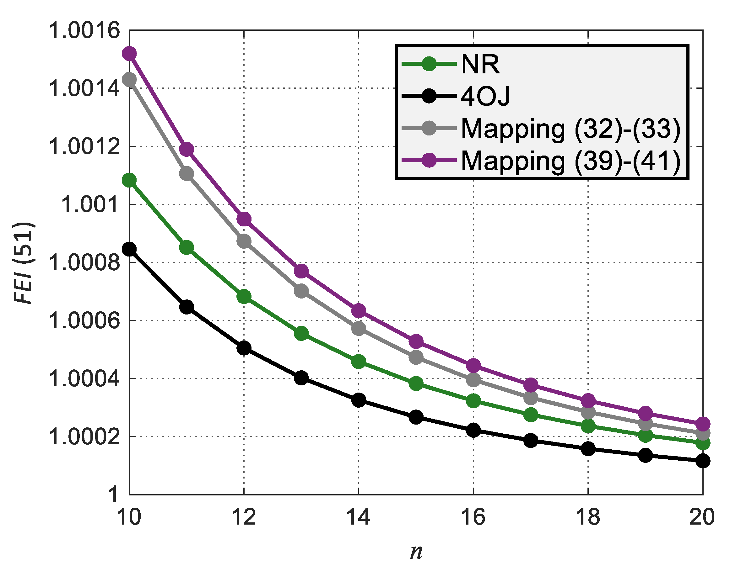
Comparing NR (mapping (2)) with the developed solvers (32) and (33) and (39)–(41), one can clearly check that the NR is more efficient since only one LU factorization is required whereas the developed techniques require two. In addition, it is clear that the developed methods involve more computations like vectors sums. However, the developed solvers achieve higher convergence rate, which presumably leads to a faster convergence. In this sense, it is difficult to analyze which approach is more efficient. To solve this issue, it is desirable to compare the developed techniques with NR and 4OJ using some measure index. Various indexes are available in the literature for comparing the efficiency of different non-linear solvers. In this case, we have considered the following one [21]:

$$FEI=p^{\raisebox{1ex}{$1$}\!\left/ \!\raisebox{-1ex}{$CO$}\right.}$$

(51)

where, $p\in {ℝ}^{+}$ is the order of convergence, and $CO$ stands for the total computational cost of an iteration in terms of flops (see [21] for further details). The Index (51) measures the degree of efficiency of a non-linear solver. If two methods are compared, the one with the highest $FEI$ would bethe most efficient (i.e., a priori). Figure 1 plots the value of (51) for NR, 4OJ, and the developed mappings (taking the values of $\alpha$, $\beta$, and $\gamma$ deduced from Theorems 2 and 3) for different system sizes ($n$). As seen from this figure, 4OJ presents the lowest efficiency index while the developed mapping (39)–(41) shows the highest one. It is also worth noting that the two developed mappings showed a better efficiency index than NR.

4. Continuous Versions of the Developed Solvers

The continuous Newton’s method [4] is based on the analogy of NR and the forward Euler method. Following this same idea, one may observe the similitude of the mappings (3) and (4), (32) and (33), and (39)–(41) with the family of Runge–Kutta formulas [22]. Thus, whereas (3) and (4) and (32) and (33) share structure with the 2-stage Runge–Kutta methods (e.g., the Trapezoidal rule), the mapping (39)–(41) keeps similar to the 3-stage Runge–Kutta formulas. This analogy allows for directly applying the continuous Newton’s framework to those techniques, thus extending their applicability to ill-conditioned problems. This way, by introducing the discrete step size $h\in {ℝ}^{+}$, the mappings (3) and (4), (32) and (33), and (39)–(41) may be respectively converted to their following continuous counterparts. In this case, we have considered the well-known Ralston’s method [22], which considers a modified version of the forward Euler formula taking 2/3 parts of the step size. Keeping this on mind, the expressions (52)–(58) represent the continuous versions of the mappings (3) and (4), (32) and (33), and (39)–(41), respectively:

$${\mathit{y}}_k={\mathit{x}}_k-\frac{2h}{3}{\left[g^{\prime }\left({\mathit{x}}_k\right)\right]}^{-1}g\left({\mathit{x}}_k\right)$$

(52)

$${\mathit{x}}_{k+1}={\mathit{x}}_k-h\left[\mathit{I}-\frac{3}{2}{\left[3g^{\prime }\left({\mathit{y}}_k\right)-g^{\prime }\left({\mathit{x}}_k\right)\right]}^{-1}\left(g^{\prime }\left({\mathit{y}}_k\right)-g^{\prime }\left({\mathit{x}}_k\right)\right)\right]{\left[g^{\prime }\left({\mathit{x}}_k\right)\right]}^{-1}g\left({\mathit{x}}_k\right)$$

(53)

$${\mathit{y}}_k={\mathit{x}}_k-\frac{2h}{3}{\left[g^{\prime }\left({\mathit{x}}_k\right)\right]}^{-1}g\left({\mathit{x}}_k\right)$$

(54)

$${\mathit{x}}_{k+1}=\frac{1}{4}{\mathit{x}}_k+\frac{3}{4}{\mathit{y}}_k-h{\left[3g^{\prime }\left({\mathit{y}}_k\right)-g^{\prime }\left({\mathit{x}}_k\right)\right]}^{-1}g\left({\mathit{x}}_k\right)$$

(55)

$${\mathit{y}}_k={\mathit{x}}_k-\frac{2h}{3}{\left[g^{\prime }\left({\mathit{x}}_k\right)\right]}^{-1}g\left({\mathit{x}}_k\right)$$

(56)

$${\mathit{z}}_k=\frac{1}{4}{\mathit{x}}_k+\frac{3}{4}{\mathit{y}}_k-h{\left[3g^{\prime }\left({\mathit{y}}_k\right)-g^{\prime }\left({\mathit{x}}_k\right)\right]}^{-1}g\left({\mathit{x}}_k\right)$$

(57)

$${\mathit{x}}_{k+1}={\mathit{z}}_k-2h{\left[3g^{\prime }\left({\mathit{y}}_k\right)-g^{\prime }\left({\mathit{x}}_k\right)\right]}^{-1}g\left({\mathit{z}}_k\right)$$

(58)

The step size can be adapted for each iteration based on the local truncation error. Exploiting the similitude of (52)–(58) with the family of Runge–Kutta techniques, the local truncation error can be estimated using the half-step method as follows:

$$\xi =\Vert {\mathit{y}}_k-{\mathit{x}}_{k+1}\Vert {}_{\infty }$$

(59)

where ${\Vert ·\Vert }_{\infty }:{ℝ}^n\to {ℝ}^{+}$ is the infinity norm. Then, (60) can be used for computing the step size using the following heuristic rule [4]:

$$if\xi >100 then h\leftarrow \max \left\{0.75h,0.5\right\}$$

$$if\xi \le 100 then h\leftarrow \min \left\{1.2h,1\right\}$$

(60)

Based on these rules, the step size increases if the truncation error is lower than a given threshold and decreases if the truncation error is greater than a given threshold. In this case, the step size is lower bounded to 0.5 for avoiding being trapped in a local minimum, while the step size is upper bounded to 1 since the considered mappings achieved their maximum convergence rate for this value. It is worth noting that if $h$ is not lower limited, the mappings (52)–(58) would provide a solution close to the feasibility of the power flow equations, as discussed in [4,12]. The section is completed by summarizing the main steps of PFC using the mapping (52) and (53) (also applicable for (54) and (55) and (56)–(58)) in the Algorithm 1 using pseudocode. Here, ${\Vert g\Vert }_{\infty }$ has been considered as convergence criterion and $\epsilon \in {ℝ}^{+}$ is the convergence tolerance. In addition, the algorithm fails if the iteration counter surpasses a given threshold $k^{\max }$, which usually indicates divergence.

Algorithm 1 main steps of PFC using (46)

1: Let ${\mathit{x}}_0$, $\epsilon$, $k^{\max }$ and $h$ be given 2: Initialize $k\leftarrow 0$ 3: while$g{\left({\mathit{x}}_k\right)}_{\infty }\ge \epsilon$ do 4:  Solve (52) and (53) # or (54) and (55), (56)–(58) 5:  if ${\Vert g\left({\mathit{x}}_k\right)\Vert }_{\infty }<\epsilon$ then 6:   break # Convergence 7:  else 8:   Update $k\leftarrow k+1$ 9:   if $k>k^{\max }$ then 10:    break # Fail 11:   end if 12:  end if 13:  Update $h$ using (60) 14: end do 15: return solution ${\mathit{x}}_k$

Stability of the Mappings (52)–(58)

The mappings (52)–(58) can be interpreted as dynamic systems, and their stabilities may be studied by calculating the eigenvalues of the Jacobian of the function $G={\mathit{x}}_{k+1}-{\mathit{x}}_k$ at ${\mathit{x}}^{*}$ [4].

For the mapping (52) and (53), one can write:

$$G=-h\left[\mathit{I}-\frac{3}{2}{\left[3g^{\prime }\left(\mathit{y}\right)-g^{\prime }\left(\mathit{x}\right)\right]}^{-1}\left(g^{\prime }\left(\mathit{y}\right)-g^{\prime }\left(\mathit{x}\right)\right)\right]{\left[g^{\prime }\left(\mathit{x}\right)\right]}^{-1}g\left(\mathit{x}\right)$$

(61)

by differentiating (61) with respect to $\mathit{x}$, one obtains:

$$\begin{gathered} {\nabla }_{\mathit{x}}G=-h\left[-\frac{3}{2}\left({\nabla }_{\mathit{x}}{\left[3g^{\prime }\left(\mathit{y}\right)-g^{\prime }\left(\mathit{x}\right)\right]}^{-1}\left(g^{\prime }\left(\mathit{y}\right)-g^{\prime }\left(\mathit{x}\right)\right)+{\left[3g^{\prime }\left(\mathit{y}\right)-g^{\prime }\left(\mathit{x}\right)\right]}^{-1}\left(g^{″}\left(\mathit{y}\right)-g^{″}\left(\mathit{x}\right)\right)\right)\right] \\ {\left[g^{\prime }\left(\mathit{x}\right)\right]}^{-1}g\left(\mathit{x}\right)-h\left[\mathit{I}-\frac{3}{2}{\left[3g^{\prime }\left(\mathit{y}\right)-g^{\prime }\left(\mathit{x}\right)\right]}^{-1}\left(g^{\prime }\left(\mathit{y}\right)-g^{\prime }\left(\mathit{x}\right)\right)\right]\left({\nabla }_{\mathit{x}}{\left[g^{\prime }\left(\mathit{x}\right)\right]}^{-1}g\left(\mathit{x}\right)+\mathit{I}\right) \end{gathered}$$

(62)

where $g^{″}={\nabla }_{\mathit{x}\mathit{x}}g\in {ℝ}^{n\times n^2}$ is the Hessian matrix of the power flow equations (see [23]). Easily, one can check that ${\mathit{y}|}_{{\mathit{x}}^{*}}={\mathit{x}}^{*}$ for (52) and (53), so, evaluating (62) at ${\mathit{x}}^{*}$ yields:

$${{\nabla }_{\mathit{x}}G|}_{{\mathit{x}}^{*}}=-h\mathit{I}$$

(63)

Equation (63) says that all the eigenvalues of ${{\nabla }_{\mathit{x}}G|}_{{\mathit{x}}^{*}}$ are negative real, which implies that ${\mathit{x}}^{*}$, if it exists, is asymptotically stable. For the mapping (54) and (55), the function $G$ cannot be directly obtained. However, since in this case ${\mathit{y}|}_{{\mathit{x}}^{*}}={\mathit{x}}^{*}$, we can write:

$${G|}_{{\mathit{x}}^{*}}=-h{\left[2g^{\prime }\left({\mathit{x}}^{*}\right)\right]}^{-1}g\left({\mathit{x}}^{*}\right)$$

(64)

and by differentiating (64) w.r.t. $\mathit{x}$, one obtains:

$${{\nabla }_{\mathit{x}}G|}_{{\mathit{x}}^{*}}=-h\left({\nabla }_{\mathit{x}}{\left[2g^{\prime }\left({\mathit{x}}^{*}\right)\right]}^{-1}g\left({\mathit{x}}^{*}\right)+{\left[2g^{\prime }\left({\mathit{x}}^{*}\right)\right]}^{-1}{g}^{\prime }\left({\mathit{x}}^{*}\right)\right)=-\frac{h}{2}\mathit{I}$$

(65)

by result (65), one can conclude that ${\mathit{x}}^{*}$ is also asymptotically stable for (54) and (55). Finally, for the mapping (56)–(58):

$$G=-h{\left[3g^{\prime }\left(\mathit{y}\right)-g^{\prime }\left(\mathit{x}\right)\right]}^{-1}g\left(\mathit{x}\right)-2h{\left[3g^{\prime }\left(\mathit{y}\right)-g^{\prime }\left(\mathit{x}\right)\right]}^{-1}g\left(\mathit{z}\right)$$

(66)

by differentiating (66) w.r.t. $\mathit{x}$, one obtains:

$${\nabla }_{\mathit{x}}G=-h\left({\nabla }_{\mathit{x}}{\left[3g^{\prime }\left(\mathit{y}\right)-g^{\prime }\left(\mathit{x}\right)\right]}^{-1}g\left(\mathit{x}\right)+{\left[3g^{\prime }\left(\mathit{y}\right)-g^{\prime }\left(\mathit{x}\right)\right]}^{-1}{g}^{\prime }\left(\mathit{x}\right)+2\left({\nabla }_{\mathit{x}}{\left[3g^{\prime }\left(\mathit{y}\right)-g^{\prime }\left(\mathit{x}\right)\right]}^{-1}g\left(\mathit{x}\right)+{\left[3g^{\prime }\left(\mathit{y}\right)-g^{\prime }\left(\mathit{x}\right)\right]}^{-1}{g}^{\prime }\left(\mathit{z}\right)\right)\right)$$

(67)

Since that ${\mathit{y}|}_{{\mathit{x}}^{*}}={\mathit{x}}^{*}$ for the mapping (56)–(58), one can assert that that ${\mathit{z}|}_{{\mathit{x}}^{*}}={\mathit{x}}^{*}$; so, this result can be substituted into (67), which yields:

$${{\nabla }_{\mathit{x}}G|}_{{\mathit{x}}^{*}}=-\frac{3}{2}h\mathit{I}$$

(68)

Since the eigenvalues of (68) have not a real positive part, one can conclude that ${\mathit{x}}^{*}$ is asymptotically stable for the mapping (56)–(58).

5. Handling with Reactive Limits of Generators

One main concern in PFC is the consideration of different equipment limits [9]. In this sense, the formulations presented on this work do not directly take into account the reactive limits at PV buses. Nonetheless, consideration of this aspect is straightforward by incorporating a common switching PV-PQ strategy, similar to other works like [6,9]. Basically, it consists on converting those PV buses with any limit violation to PQ, taking the limit hit as injected reactive power. The proposed strategy is summed in the following steps.

(1)

Firstly, the power flow is solved by ignoring the reactive limits. After that, it is checked if any limit violation at PV buses occurs. If not, the process is ended and the solution ${\mathit{x}}_k$ is declared feasible; otherwise go to step 2.

(2)

Those PV buses are converted to PQ. For those, the violated reactive limit is taken as the new injected reactive power, and the voltage magnitude is incorporated into the unknown vector as a variable.

(3)

Taking ${\mathit{x}}_k$ as starting point, the power flow problem is solved, then go to step 1.

If there are not PV buses in Step 1, the problem is declared unfeasible since there does not exist a solution in which the reactive limits are not violated. It is worth noting that similar strategies can be considered for incorporating other functional limits or controls.

6. Numerical Experiments

Along the developed methods (32) and (33) and (39)–(41) (with $\alpha =\frac{1}{4}$, $\beta =\frac{3}{4}$ and $\gamma =2$), NR, 4OJ, and the Reverse-Bulirsch–Stoer algorithm (RBS) [6] have been implemented in polar coordinates on Matpower [24]. The Algorithm 1 has been followed as benchmark for implementing the tested solvers, omitting the line 13 when not needed and replacing (52) and (53) in line 4 by the mapping considered. Various realistic systems such as the 69-bus radial network, the 2000-bus Texas synthetic grid along various portions of the Polish and the European transmission systems have been considered [25,26,27]. The tested networks have been denoted by the name used in Matpower (see [28] for details). All simulations have been carried out from a flat start, taking $\epsilon ={10}^{-5}$ and $k^{\max }=1000$.

6.1. Convergence Rates for Well-Conditioned Cases

Table 1. Total iterations for well-conditioned cases.

Case	NR	RBS	4OJ	(32) and (33)	(39)–(41)
case69	3	8	2	2	1
case_ACTIVSg2000	5	12	3	3	2
case3120sp	5	13	3	3	2
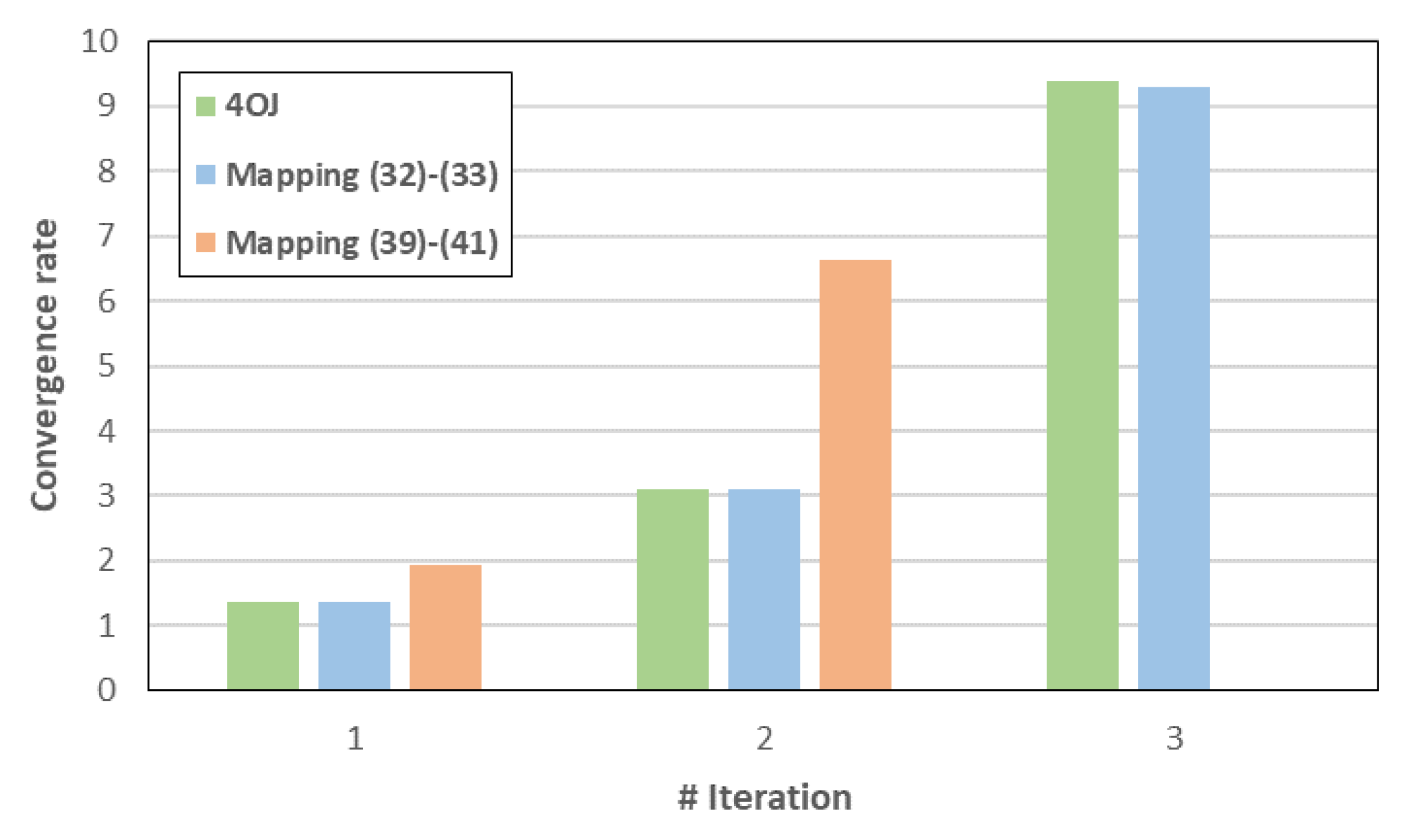
case9241pegase	5	13	3	3	2

presents the total iterations for different realistic well-conditioned cases ignoring the reactive limits. As seen in this table, the developed mappings alongside 4OJ were able to converge faster than the other tested solvers. This was expected since NR has quadratic convergence while RBS usually converges linearly due to the influence of the step size, while 4OJ and (32) and (33) have 4th order of convergence and (39)–(41) has 6th order of convergence. Figure 2 shows the convergence rate of 4OJ and the mappings (32) and (33) and (39)–(41) in the ‘case9241pegase’. As observed, 4OJ and the mapping (32) and (33) converged linearly for the first iteration, while the mapping (39)–(41) converged almost quadratically. In the second iteration, 4OJ and the mapping (32) and (33) achieved 3rd order of convergence while the mapping (39)–(41) achieved 6th order of convergence and reached the required convergence tolerance. For the third iteration, when the algorithms have evolved very close to the solution, 4OJ and the mapping (32) and (33) achieved 9th order of convergence. These results demonstrate the local convergence characteristics of the studied techniques. Nevertheless, the developed mapping (39)–(41) has shown superior convergence features than 4OJ and (32) and (33).

6.2. Convergence Rates for Ill-Conditioned Cases

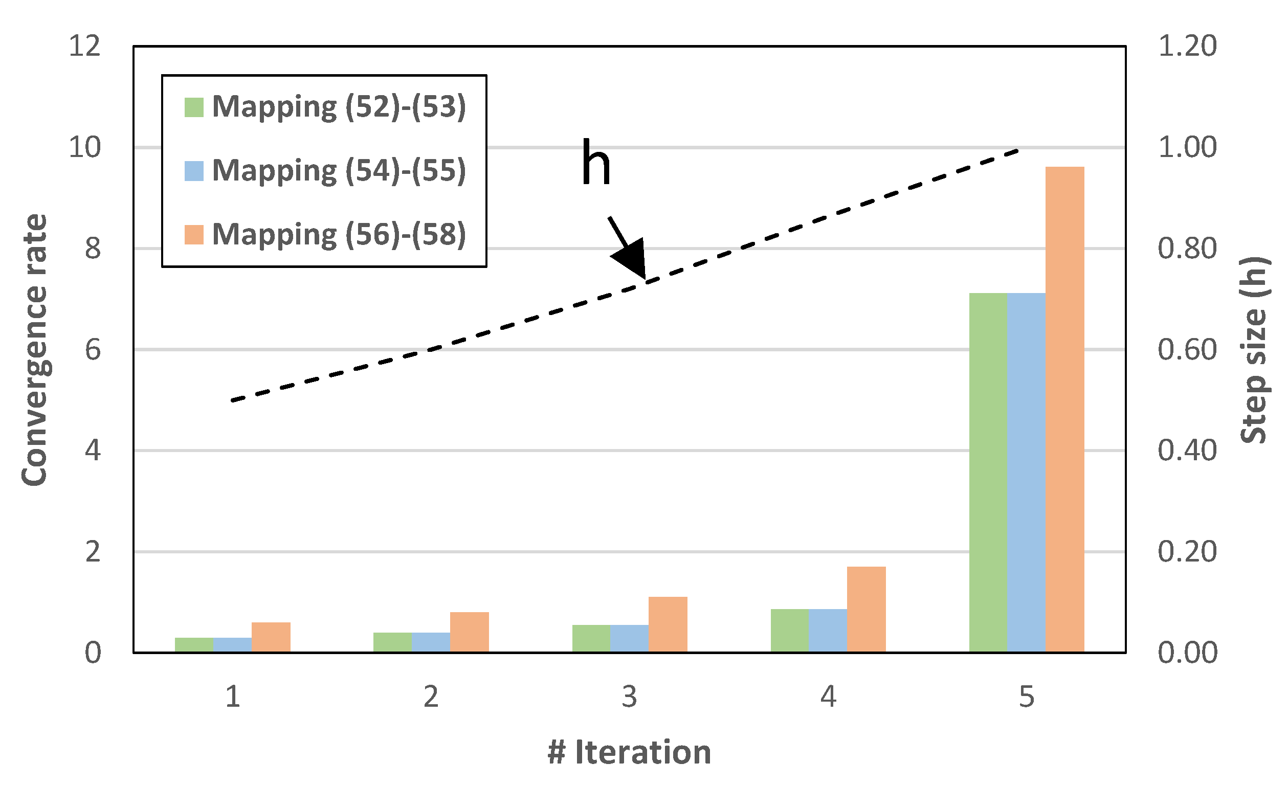
Next, let us study how the continuous methods (52)–(58) perform in some ill-conditioned cases.

Table 2. Total iterations of various continuous methods for ill-conditioned cases.

Case	SRM [4]	RBS	(52) and (53)	(54) and (55)	(56)–(58)
Case3012wp	27	13	5	5	5
Case3375wp	27	13	5	5	5

shows the total iterations of these methods along the continuous implementation of NR (‘Simple Robust Method’ (SRM) in [4]) and RBS, in two snapshots of the Polish transmission system (these systems are ill-conditioned as reported in [6] according to the Definition 1, so that NR, 4OJ, (32) and (33), and (39)–(41) fail for solving them). As in preceding simulations, the reactive limits are ignored in this case. For NR and the mappings (52)–(58), the step size is initialized equal to 0.5, while the guidelines in [6] have been followed for RBS. In the studied cases, SRM performed poorly, employing a huge amount of iterations for converging, while the developed mappings were the most competitive. Figure 3 shows the convergence rate of the mappings (52)–(58) for the ‘case3012wp’ along the value of the step size each iteration. As observed, these techniques performed linearly when $h$ was short. As the algorithms evolved, the step size was enlarged by making use of the rule (60) up to be equal to 1, then, the mappings (52)–(58) quickly achieved high convergence rates due to the algorithms are already evolving close to the solution.

6.3. Convergence Rates for Limit Cases

The loading level of a system may affect the performance and reliability of a power flow solution method. In this regard, that loading level closest to the point of collapse supposes the most demanding conditions from a power flow solver. We have studied the performance of the considered techniques for such a point (limit loading level namely ${\lambda }^{\lim }$). The limit loading level for each system has been calculated using the continuation power flow [13].

Table 3. Total iterations for well-conditioned cases with limit load conditions.

Case	${\mathit{\lambda }}^{\mathit{l}\mathit{i}\mathit{m}}$	NR	RBS	4OJ	(32) and (33)	(39)–(41)
case69	3.2116	8	9	7	7	4
case_ACTIVSg2000	1.0236	9	12	5	5	4
case3120sp	1.5653	11	13	6	6	5
case9241pegase	1.0767	10	13	5	5	4

and

Table 4. Total iterations for ill-conditioned cases with limit load conditions.

Case	${\mathit{\lambda }}^{\mathit{l}\mathit{i}\mathit{m}}$	SRM [4]	RBS	(52) and (53)	(54) and (55)	(56)–(58)
Case3012wp	1.2734	27	13	7	7	6
Case3375wp	1.1586	27	13	7	7	6

provide the total iterations for well and ill-conditioned cases with limit loading conditions, respectively, ignoring the reactive limits at PV buses. Regarding well-conditioned cases, the mapping (39)–(41) required fewer iterations than NR, RBS, 4OJ, and the mapping (32) and (33). As expected, 4OJ and the mapping (32) and (33) required the same number of iterations due to its 4th order of convergence. In ill-conditioned cases, the mapping (56)–(58) was the most competitive.

6.4. Convergence Rates with Reactive Limits

Next, the total iterations with reactive limits at PV buses are presented in

Table 5. Total iterations for well-conditioned cases with reactive limits.

Case	NR	RBS	4OJ	(32) and (33)	(39)–(41)
case69	3	8	2	2	1
case_ACTIVSg2000	13	39	8	8	5
case3120sp	13	48	8	8	6
case9241pegase	12	41	7	7	5

and

Table 6. Total iterations for ill-conditioned cases with reactive limits.

Case	SRM [4]	RBS	(52) and (53)	(54) and (55)	(56)–(58)
Case3012wp	53	29	15	15	13
Case3375wp	57	32	19	19	16

for well and ill-conditioned cases, respectively. These limits have been incorporated in the tested methods using the strategy described in Section 5. As observed, the mapping (39)–(41) required the least number of iterations in well-conditioned cases, while 4OJ and the mapping (32) and (33) outperformed NR and RBS in all cases. For ill-conditioned cases, the mapping (56)–(58) required fewer iterations than SRM, RBS, and the mappings (52)–(55). It is worth noting that these two latter techniques outperformed SRM and RBS in all cases.

6.5. Solution Times

Table 7. Solution times (ms) for well-conditioned cases.

Case	NR	RBS	4OJ	(32) and (33)	(39)–(41)
case69	3.66	23.21	6.96	4.22	2.34
case_ACTIVSg2000	70.73	542.04	7764.41	84.46	60.16
case3120sp	96.82	800.57	18,625.39	113.15	79.51
case9241pegase	320.10	2677.31	629,536.74	379.32	265.16

,

Table 8. Solution times (ms) for ill-conditioned cases.

Case	SRM [4]	RBS	(52) and (53)	(54) and (55)	(56)–(58)
Case3012wp	473.65	767.98	21,374.45	178.03	183.12
Case3375wp	524.10	848.08	26,557.90	196.71	201.40

,

Table 9. Solution times (ms) for well-conditioned cases with limit load conditions.

Case	NR	RBS	4OJ	(32) and (33)	(39)–(41)
case69	9.76	26.10	24.36	14.77	9.36
case_ACTIVSg2000	127.35	542.04	9705.50	140.75	120.32
case3120sp	212.96	800.54	27,938.10	226.32	198.80
case9241pegase	640.20	2677.35	629,536.75	632.20	530.32

,

Table 10. Solution times (ms) for ill-conditioned cases with limit load conditions.

Case	SRM [4]	RBS	(52) and (53)	(54) and (55)	(56)–(58)
Case3012wp	473.58	768.04	29,924.23	249.27	219.72
Case3375wp	524.07	848.12	37,181.06	275.38	241.68

,

Table 11. Solution times (ms) for well-conditioned cases with reactive limits.

Case	NR	RBS	4OJ	(32) and (33)	(39)–(41)
case69	3.66	23.21	6.96	4.22	2.34
case_ACTIVSg2000	183.95	1761.63	15,528.80	225.20	150.40
case3120sp	251.68	2955.84	37,250.80	301.76	238.56
case9241pegase	768.24	8443.95	881,351.45	885.08	662.90

and

Table 12. Solution times (ms) for ill-conditioned cases with reactive limits.

Case	SRM [4]	RBS	(52) and (53)	(54) and (55)	(56)–(58)
Case3012wp	929.62	1713.32	64,123.35	534.15	476.06
Case3375wp	1106.37	2087.68	100,920.02	747.46	644.48

provide the solution times for the simulations reported in Table 1, Table 2, Table 3, Table 4, Table 5 and Table 6, respectively. These results have been obtained on a 64-bit i5-9400F Intel Core personal computer (2.90 GHz, 8 GB of RAM), as the average value of 100 simulations.

For well-conditioned cases, the mapping (32) and (33) was occasionally slower than NR, which may be contradictory with the conclusions of Section 3.3. For explaining that, one should note the total amount of LU factorizations required by each method. Since it is the heaviest part of NR and the mapping (32) and (33), the required solution time will be quite proportional to the total amount of these calculations. For example, the mapping (32) and (33) needed six factorizations for the ‘case_ACTIVSg2000′, while NR needed five. It also explains why the mapping (39)–(41) was the most competitive technique while RBS needed six factorizations for the first iteration, four iterations for the second, and two for each remainder iteration; thus, it was required for the ‘case_ACTIVSg2000′ 30 factorizations in total. The reason behind the low efficiency of 4OJ was, as commented, the solution of a matrix system.

Similar conclusions can be extracted for RBS in ill-conditioned cases. Here, SRM turned out to be inefficient due to the large number of iterations needed. The mapping (52) and (53), as 4OJ, was very inefficient due to the calculation of a matrix system.

For limit load conditions and reactive limits enforcement, the mapping (39)–(41) was the most efficient in well-conditioned cases, while the mapping (56)–(58) was the winner in ill-conditioned cases.

7. Potential Applications of the Developed Solvers

The developed nonlinear solvers introduced in this paper are focused on PFC. To validate them, various realistic systems have been tested and the results were promising. However, the developed techniques can find other applications that may be valuable for real-life tools. Further analysis of such applications is out of scope of this paper, but this section is dedicated to overview them.

In the area of electrical engineering, the developed solvers could offer good results in other related tools. For example, the so-called continuation power flow (CPF) [13] is performed in two stages called predictor and corrector. During the corrector stage, the power flow problem is solved. This process is repeated various times until the whole continuation curve is drawn, which may imply many PFCs and therefore the whole process can be very time-consuming. Recent studies [29] have demonstrated that the usage of HONL techniques may alleviate the computational cost of CPF, which may suppose an unvaluable contribution for real-time security tools, in which CPF is widely employed.

Water (or liquid) flow models are usually nonlinear [30,31]. To analyze dynamics behavior of water flow, some models based on differential equations, such as the Richards equations, can be linearized, and then solved using iterative methods. In [31], NR, Picard iteration, and L-scheme methods were compared for this problem showing that not only computational efficiency, but also numerical stability are important in water flow problems. In this area, the developed solvers and their continuous counterparts may offer very good performance. Indeed, while the mappings (32) and (33) and (39)–(41) have been proved to be more efficient than NR, the continuous mappings (52)–(58) can offer good numerical stability in ill-posed problems.

Finally, computational efficiency is of great interest to solve nonlinear coefficient inverse problems for partial differential equations. Especially when the coefficients are time-dependent and therefore various systems have to be solved, usually in real-time applications. Clear examples of these kinds of problems are the Moore–Gibson–Thompson equation [32] or the the nonlinear Oskolkov’s system [33].

8. Conclusions and Future Works

This paper deals with the applicability of 4OJ for PFC. This technique is not computationally competitive, at least in realistic systems, due to its high computational cost; more specifically, the solution of a matrix system involved in the solution procedure of 4OJ makes this technique unattractive for industry tools. Motivated by this issue, the authors of this paper have proposed two modifications of 4OJ, which aim at circumventing the computational issues manifested by 4OJ. The new methodologies focus on eliminating the matrix system, replacing it with cheaper calculations like solution linear systems. The new proposals have 4th and 6th order of convergence and present a better efficiency index.

Additionally, this paper has discussed the continuous counterparts of 4OJ and the developed methods. These formulations aim at extending the applicability of the developed solvers to ill-conditioned cases, which are more frequently observed nowadays. Thereby, the new proposals suppose a valuable contribution for industry tools.

Extensive numerical experiments have been performed. The developed techniques have been compared with NR, 4OJ, SRM, and RBS. Both well and ill-conditioned systems have been contemplated for analyzing the performance of the developed solvers and their continuous counterparts. Results revealed the superiority of the new proposals compared with other traditional PF solvers. The new methodologies outperformed NR and RBS in all studied cases in both convergence rates and solution times. An in-depth comparison with 4OJ revealed the clear superiority of our methods and serves to highlight the difficulties of 4OJ to be applied to PF analysis.

Future works should be devoted to validating the novel techniques in other related problems such as those reviewed in Section 7, thus, as other PF formulations like [15,17] or [18].

References

- Karimi, M.; Shahriari, A.; Aghamohammadi, M.R.; Terzija, V. Application of Newton-based load flow methods for determining steady-state condition of well and ill-conditioned power systems: A review. Int. J. Elect. Power Energy Syst. 2019, 113, 298–309. [Google Scholar] [CrossRef]
- Tang, K.; Dong, S.; Shen, J.; Zhu, C.; Song, Y. A Robust and Efficient Two-Stage Algorithm for Power Flow Calculation of Large-Scale Systems. IEEE Trans. Power Syst. 2019, 34, 5012–5022. [Google Scholar] [CrossRef]
- Xie, N.; Torelli, F.; Bompard, E.; Vaccaro, A. Dynamic computing paradigm for comprehensive power flow analysis. IET Gener. Transmiss. Distrib. 2013, 7, 832–842. [Google Scholar] [CrossRef]
- Milano, F. Continuous Newton’s Method for Power Flow Analysis. IEEE Trans. Power Syst. 2009, 24, 50–57. [Google Scholar] [CrossRef]
- Pourbagher, R.; Derakhshandeh, S.Y. Application of high-order Levenberg-Marquardt method for solving the power flow problem in the ill-conditioned systems. IET Gener. Transmiss. Distrib. 2016, 10, 3017–3022. [Google Scholar] [CrossRef]
- Tostado-Véliz, M.; Kamel, S.; Jurado, F. A Robust Power Flow Algorithm Based on Bulirsch-Stoer Method. IEEE Trans. Power Syst. 2019, 34, 3081–3089. [Google Scholar] [CrossRef]
- Milano, F. Implicit Continuous Newton Method for Power Flow Analysis. IEEE Trans. Power Syst. 2019, 34, 3309–3311. [Google Scholar] [CrossRef]
- Derakhshandeh, S.Y.; Pourbagher, R. Application of high-order Newton-like methods to solve power flow equations. IET Gener. Transmiss. Distrib. 2016, 10, 1853–1859. [Google Scholar] [CrossRef]
- Tostado-Véliz, M.; Kamel, S.; Jurado, F. A Novel Family of Efficient Power-Flow Methods With High Convergence Rate Suitable for Large Realistic Power Systems. IEEE Syst. J. 2021, 15, 738–746. [Google Scholar] [CrossRef]
- Tostado-Véliz, M.; Kamel, S.; Alquthami, T.; Jurado, F. A Three-Stage Algorithm Based on a Semi-Implicit Approach for Solving the Power-Flow in Realistic Large-Scale ill-Conditioned Systems. IEEE Access 2020, 8, 35299–35307. [Google Scholar] [CrossRef]
- Iwamoto, S.; Tamura, Y. A Load Flow Calculation Method for Ill-Conditioned Power Systems. IEEE Trans. Power Appar. Syst. 1981, PAS-100, 1736–1743. [Google Scholar] [CrossRef]
- Overbye, T.J. A power flow measure for unsolvable cases. IEEE Trans. Power Syst. 1994, 9, 1359–1365. [Google Scholar] [CrossRef]
- Zhang, X.-P.; Ju, P.; Handschin, E. Continuation three-phase power flow: A tool for voltage stability analysis of unbalanced three-phase power systems. IEEE Trans. Power Syst. 2005, 20, 1320–1329. [Google Scholar] [CrossRef]
- Milano, F. Analogy and Convergence of Levenberg’s and Lyapunov-Based Methods for Power Flow Analysis. IEEE Trans. Power Syst. 2016, 31, 1663–1664. [Google Scholar] [CrossRef]
- Saleh, S.A. The Formulation of a Power Flow Using d-q Reference Frame Components-Part I: Balanced 3 Systems. IEEE Trans. Ind. Appl. 2016, 52, 3682–3693. [Google Scholar] [CrossRef]
- Cordero, A.; Villalba, E.G.; Torregrosa, J.R.; Triguero-Navarro, P. Convergence and Stability of a Parametric Class of Iterative Schemes for Solving Nonlinear Systems. Mathematics 2021, 9, 86. [Google Scholar] [CrossRef]
- Penido, D.R.R.; de Araujo, L.R.; Carneiro, S.; Pereira, J.L.R.; Garcia, P.A.N. Three-Phase Power Flow Based on Four-Conductor Current Injection Method for Unbalanced Distribution Networks. IEEE Trans. Power Syst. 2008, 23, 494–503. [Google Scholar] [CrossRef]
- Pires, R.; Mili, L.; Chagas, G. Robust complex-valued Levenberg-Marquardt algorithm as applied to power flow analysis. Int. J. Elect. Power Energy Syst. 2019, 113, 383–392. [Google Scholar] [CrossRef]
- Khirallah, M.Q.; Hafiz, M.A. Solving system of non-linear equations using family of Jarratt methods. Int. J. Differ. Equ. App. 2013, 12, 2–69. [Google Scholar] [CrossRef]
- Traub, J.F. Iterative Methods for the Solution of Equations; Chelsea: New York, NY, USA, 1982. [Google Scholar]
- Cordero, A.; Hueso, J.L.; Martínez, E.; Torregrosa, J.R. A modified Newton-Jarratt’s composition. Numer. Algor. 2010, 5, 87–99. [Google Scholar] [CrossRef]
- Butcher, J.C. Numerical Methods for Ordinary Differential Equations; Wiley: Hoboken, NJ, USA, 2003. [Google Scholar]
- Iwamoto, S.; Tamura, Y. A Fast Load Flow Method Retaining Nonlinearity. IEEE Trans. Power Appar. Syst. 1978, PAS-97, 1586–1599. [Google Scholar] [CrossRef]
- Zimmerman, R.D.; Murillo-Sánchez, C.E.; Thomas, R.J. Matpower: Steady-State Operations, Planning and Analysis Tools for Power Systems Research and Education. IEEE Trans. Power Syst. 2011, 26, 12–19. [Google Scholar] [CrossRef] [Green Version]
- Birchfield, A.B.; Xu, T.; Gegner, K.M.; Shetye, K.S.; Overbye, T.J. Grid Structural Characteristics as Validation Criteria for Synthetic Networks. IEEE Trans. Power Syst. 2017, 32, 3258–3265. [Google Scholar] [CrossRef]
- Josz, C.; Fliscounakis, S.; Maeght, J.; Panciatici, P. AC Power Flow Data in Matpower and QCQP Format: iTesla, RTE Snapshots, and PEGASE. arXiv 2016. Available online: https://arxiv.org/abs/1603.01533 (accessed on 9 June 2021).
- Fliscounakis, S.; Panciatici, P.; Capitanescu, F.; Wehenkel, L. Contingency Ranking with Respect to Overloads in Very Large Power Systems Taking into Account Uncertainty, Preventive, and Corrective Actions. IEEE Trans. Power Syst. 2013, 28, 4909–4917. [Google Scholar] [CrossRef] [Green Version]
- Matpower User’s Manual. Available online: https://matpower.org/docs/manual.pdf (accessed on 9 June 2020).
- Tostado-Véliz, M.; Kamel, S.; Jurado, F. Development and Comparison of Efficient Newton-Like Methods for Voltage Stability Assessment. Elect. Power Comp. Syst. 2020, 48, 1798–1813. [Google Scholar] [CrossRef]
- Difonzo, F.V.; Masciopinto, C.; Vurro, M.; Berardi, M. Shooting the Numerical Solution of Moisture Flow Equation with Root Water Uptake Models: A Python Tool. Water Res. Manag. 2021, 35, 2553–2567. [Google Scholar] [CrossRef]
- Illiano, D.; Pop, I.S.; Radu, F.A. Iterative schemes for surfactant transport in porous media. Comput. Geosci. 2021, 25, 805–822. [Google Scholar] [CrossRef]
- Tekin, I. Inverse problem for a nonlinear third order in time partial differential equation. Math. Methods Appl. Sci. 2021, 44, 9571–9581. [Google Scholar] [CrossRef]
- Fedorov, V.E.; Ivanova, N.D. Inverse problem for Oskolkov’s system of equations. Math. Methods Appl. Sci. 2017, 40, 6123–6126. [Google Scholar] [CrossRef]
Figure 1.
Value of the efficiency index (51) for NR, 4OJ, and the developed methods (32) and (33) and (39)–(41).
Figure 2.
Convergence rates of 4OJ and the developed methods for the ‘case9241pegase’.
Figure 3.
Step size and convergence rates of 4OJ and the developed methods for the ‘case3012wp’.