
Enhanced Brain Storm Optimization Algorithm Based on Modified Nelder–Mead and Elite Learning Mechanism


1
School of Computer Science and Engineering, Xi’an University of Technology, Xi’an 710048, China
2
Shaanxi Key Laboratory for Network Computing and Security Technology, Xi’an 710048, China
3
College of Information and Communication, National University of Defense Technology, Wuhan 430035, China
*
Author to whom correspondence should be addressed.
Mathematics 2022, 10(8), 1303; https://0-doi-org.brum.beds.ac.uk/10.3390/math10081303
Submission received: 14 March 2022
/
Revised: 11 April 2022
/
Accepted: 12 April 2022
/
Published: 14 April 2022
(This article belongs to the Special Issue Evolutionary Computation 2022)
Abstract
:Brain storm optimization algorithm (BSO) is a popular swarm intelligence algorithm. A significant part of BSO is to divide the population into different clusters with the clustering strategy, and the blind disturbance operator is used to generate offspring. However, this mechanism is easy to lead to premature convergence due to lacking effective direction information. In this paper, an enhanced BSO algorithm based on modified Nelder–Mead and elite learning mechanism (BSONME) is proposed to improve the performance of BSO. In the proposed BSONEM algorithm, the modified Nelder–Mead method is used to explore the effective evolutionary direction. The elite learning mechanism is used to guide the population to exploit the promising region, and the reinitialization strategy is used to alleviate the population stagnation caused by individual homogenization. CEC2014 benchmark problems and two engineering management prediction problems are used to assess the performance of the proposed BSONEM algorithm. Experimental results and statistical analyses show that the proposed BSONEM algorithm is competitive compared with several popular improved BSO algorithms.
Keywords:
brain storm optimization algorithm; Nelder–Mead; elite learning; opposition based learningMSC:
901. Introduction
In recent years, as an effective class of optimization methods, swarm intelligence (SI) optimization algorithms are becoming more and more popular in solving complex practical problems in the fields of scientific research and engineering applications. Based on the concepts of self-organized coordination in natural swarm systems, the SI algorithms transfer information through communication with multiple local individuals to reach a common global goal collaboratively. Therefore, the collective behaviors are the core design of swarm intelligence algorithms for optimization problems [1]. For the SI algorithms, the solutions of the optimization problem are regarded as individuals of the population, and the population evolves continually via group collaboration. Some popular SI algorithms include ant colony optimization (ACO) [2], particle swarm optimization (PSO) [3], artificial bee colony optimization (ABC) [4], biogeography-based optimization (BBO) [5], cuckoo search (CS) [6], bat algorithm (BA) [7], etc. Moreover, some new optimization algorithms are proposed to solve optimization problems, such as an improved moth-flame optimization algorithm(I-MFO) [8], arithmetic optimization algorithm (AOA) [9], migration-based moth-flame optimization algorithm (M-MFO) [10], aquila Optimizer (AO) [11], red fox optimization algorithm (RFO) [12], remora optimization algorithm (ROA) [13], and chaos cloud quantum bat hybrid optimization algorithm (CCQBA) [14].
The brain storm optimization algorithm (BSO) [15] proposed by Shi in 2011 imitates the thinking and learning process of human beings to solve complex tasks. In the BSO, the population (ideas or solutions) is divided into several clusters. On the one hand, each parent idea is generated by learning from other ideas in intracluster or intercluster. On the other hand, the new idea is generated by a random search operator on the parent idea. Research findings indicate that the BSO algorithm has been successfully applied to solve optimization problems in different fields, such as feature selection [16], power system fault diagnosis [17], data classification [18], stock price forecasting [19], visual fixation prediction [20], Loney’s solenoid problem [21], electromagnetic applications [22], networks [23], and multimodal optimization [24].
In the BSO, the challenge can be mainly attributed to the effective balance mechanism between exploration and exploitation, and overexploitation may lead to premature convergence [25]. Then, different variants of BSO are proposed to improve the diversity or convergence of the algorithm, which can be mainly divided into two categories.
One category focuses on developing effective clustering methods. K-means is one of the popular clustering methods. For example, Bezdan et al. [26] proposed a hybrid swarm intelligence algorithm with a K-means algorithm to solve text clustering. The original BSO algorithm uses K-means clustering method, which has a high computational cost. In order to reduce the computational complexity, Zhan et al. [27] proposed a simple grouping method (SGM), where the seed of each group keeps unchanged to alleviate computational burden. Zhu et al. [28] proposed K-medians clustering method, which takes the median of the individuals, rather than the average value, as the new cluster center. Cao et al. [29] proposed a random grouping strategy, where a new dynamic step-size parameter control strategy is employed in the idea generation process. Chen et al. [30] proposed the role-playing strategy, which divides all ideas into three categories, namely innovative ideas, conservative ideas and common ideas. Shi [31] proposed a novel algorithm called brain storm optimization algorithm in objective space (BSO-OS). In the BSO-OS, instead of using the clustering algorithm, the convergent operation is implemented in the objective space to divide all individuals into two categories, namely elitists and normal.
The other category focuses on designing new learning strategies. To solve the problems, such as that the transfer function used in the BSO may not effectively capture the search features well, and the global search ability is poor when the search range is large, the idea difference strategy (IDS) is designed in a modified brain storm optimization (MBSO) algorithm [27]. Zhou et al. [32] proposed a step-size adaptive strategy, which is dynamically adjusted according to the current state of the individuals. If the individuals are aggregated, the step-size is relatively small. Otherwise, the step-size is relatively large. Cheng et al. [33] proposed the partial re-initialization strategy to alleviate premature convergence in the BSO algorithm. In detail, a certain number of solutions are re-initialized at each given iteration. Moreover, the number of re-initialized solutions decreases linearly at each re-initialization. Shen et al. [34] proposed an adaptive learning strategy, which guides the individual to learn from the global best individual and its cluster center, so as to improve the search ability and stability of the proposed algorithm. El-Abd proposed a global-best brain storm optimization algorithm (GBSO) [35], which uses the global-best idea information to update the population.
The basic BSO algorithm has the following disadvantages. (1) The greedy selection strategy is used to select the next population. If the population evolution deviates from the direction of global optimal solution, it may increase the possibility of falling into the local optimal solution. (2) The random noise disturbance operator [36] is used to generate new ideas; however, it is difficult for the operator to make use of potential valuable information in the search process. (3) The construction of Sselect depends largely on the center of a cluster. In some worse cases, a cluster with a local optimal solution may cause a premature convergence. Therefore, it is necessary to improve the exploitation ability of the algorithm to record the historical optimal solution and search near the historical optimal solution.
Some weaknesses of the basic BSO have been overcome by proposing new clustering method or designing new learning strategy. However, the imbalance of exploration and exploitation is still a key issue for the performance of the algorithm. Moreover, to the best of our knowledge, the Nelder–Mead simplex search method [37] has not been used in the BSO before. Based on the above discussion, we propose an enhanced BSO algorithm based on modified Nelder–Mead and elite learning mechanism (BSONME) to solve these weak points. The main contribution of the proposed BSONME algorithm are as follows.
- (1)
- The basic Nelder–Mead method is modified and used as a local searcher to explore more promising search direction for the population, so as to reduce the probability of falling into local optimum;
- (2)
- An elite learning mechanism based on Euclidean distance is proposed to update the population with a certain probability. The evolution information hidden in the elite individuals is integrated into the population, which improves the convergence of the algorithm;
- (3)
- The reinitialization strategy is employed when the population is at the stagnation stage. The well-directed and revolutionary jumping can help the population jump out of the local optimum with a large probability, so as to explore a new evolutionary direction;
- (4)
- CEC2014 contest benchmark problems and two engineering prediction problems are used to evaluate the performance of the proposed algorithm.
The structure of this paper is as follows. The original BSO algorithm and the Nelder–Mead method are briefly introduced in Section 2. The proposed BSONME algorithm is described in Section 3. In Section 4, experiments on CEC2014 benchmark problems are given. Moreover, two practical engineering problems are used to evaluate the performance of the proposed BSONME. Section 5 summarizes the whole work and puts forward the next research direction.
2. Preliminaries
2.1. Brain Storm Optimization Algorithm
Similar to other SI algorithms, the population is composed of N D-dimensional individuals in the BSO algorithm. Each individual Xi is termed as an idea, i.e., candidate solution. First, the population is initialized randomly. Then, the BSO algorithm performs a loop of optimization operations: clustering, parent idea construction, new idea generation, and selection.
- (1)
- Clustering: At each generation, the population is divided into M clusters according to K-means algorithm. Each cluster selects the best idea as its center;
- (2)
- Parent idea construction: According to the probability index, one or two clusters are used to construct the parent individual Xselect.
One situation is that Xselect is generated from two clusters. First, two different clusters are randomly selected based on the given probability. Next, there are two methods to generate the individual Xselect. One method is that Xselect is generated based on a linear combination of two centers from two different clusters. The other method is that Xselect is generated based on a linear combination of two ideas from two different clusters.
The other situation is that Xselect is generated from one cluster. The cluster is selected according to the roulette strategy. In other words, the more ideas in the cluster, the higher the probability of being selected. The probability of selecting jth cluster pj is defined as follows:
where M is the number of clusters, |Mj| is the size of the jth cluster, and N is the population size.
- (3)
- New idea generation: After parent idea Xselect is generated, a new idea is generated according to the following formula:where Xselect,d is the dth dimension of the selected idea. Xnew,d is the dth dimension of newly generated idea. N (μ, σ) is the Gaussian distribution function with mean μ and variance σ, and is defined as follows:where is the maximum number of iterations. is the current number of iterations, and is the slope coefficient, which is used to control the convergence speed of the algorithm. rand (0,1) is a number randomly distributed in the range of [0, 1]. logsig() is a sigmoid activation function.
It can be seen from Equation (3) that decreases gradually as the increase of the number of iterations. Thus, the algorithm focuses on exploration in the early stage of evolution, and focuses on exploitation in the later stage of evolution.
- (4)
- Selection: The greedy selection strategy is used to select the better one from the parent idea Xi and the newly generated idea Xnew according to their fitness. The better one is kept as a parent idea in the next generation.
The pseudo code of BSO algorithm is described by Algorithm 1.
| Algorithm 1 The BSO algorithm | |
| 1: | Randomly generate N individuals |
| 2: | Evaluate N individuals |
| 3: | while the termination criteria are not met do |
| 4: | Divide N individuals into M clusters by K-means |
| 5: | Select the cluster center for each cluster |
| 6: | if rand < p1 then |
| 7: | Randomly generated an individual to replace a selected cluster center |
| 8: | end if |
| 9: | for each individual Xi do |
| 10: | if rand < pone then |
| 11: | Select one cluster c according to Equation (1) |
| 12: | if rand < pone_center then |
| 13: | Xselect ← the center of the cluster c |
| 14: | else |
| 15: | Xselect ← Random select an individual from cluster c |
| 16: | end if |
| 17: | else |
| 18: | Randomly select two clusters c1 and c2 |
| 19: | if rand < ptwo_center then |
| 20: | Generate Xselect according to linear combination rule |
| 21: | else |
| 22: | Randomly select an individual from X1 and X2, respectively |
| 23: | Generate Xselect according to linear combination rule |
| 24: | end if |
| 25: | end if |
| 26: | Generate new idea Xnew according to Equation (2) |
| 27: | if f(Xnew) < f(Xi)then |
| 28: | Xi ←Xnew |
| 29: | f(Xi) ← f(Xnew) |
| 30: | end if |
| 31: | end for |
| 32: | end while |
2.2. Nelder–Mead Method
The Nelder–Mead method [37], proposed by Nelder et al., is a simplex search method for multidimensional unconstrained minimization. The Nelder–Mead method includes four key operations: reflection, expansion, contraction and shrinkage.
At first, (n + 1) points x1, x2, …, xn+1 are initialized in the D-dimension search space. These points are sorted in ascending order according to their fitness values.
The centroid point composed of the first points is calculated according to the formula:
Then, the reflection point xr is given as follows:
where is the reflection coefficient, and xn+1 is the worst point.
Next, the expansion point xe is calculate according to the formula:
where χ > max{1, ρ} is the expansion coefficient.
If the fitness of the reflection point xr is worse than that of the second worst xn, it is necessary to perform outside contraction or inside contraction. Here, the fitness of a point refers to its function value. When the fitness of the reflection point xr is better than that of the worst point xn+1, the outside contraction operation is performed as follows.
Otherwise, the inside contraction operation is performed as follows.
where 0 < γ < 1 is the contraction coefficient.
If the fitness of the outside contraction point xoc is worse than that of the reflection point xr, or the fitness of the inside contraction point xic is worse than that of xn+1, the shrink operation for ith point xi is performed as follow.
where 0 < σ< 1 is the shrink coefficient. The detailed information of the above mentioned four coefficients can be found in [37].
3. Proposed Method
3.1. Motivations
As mentioned before, the convergent operation and the population generation strategy used in the BSO algorithm may not be able to effectively adjust the exploration and exploitation search [36]. Therefore, the variants of BSO are proposed, such as MBSO, the improved random grouping BSO (IRGBSO) [38], and BSO-OS. MBSO proposed a new population generation strategy. IRGBSO introduced the re-initialized ideas. BSO-OS developed an effective grouping method. In order to evaluate the performance of the variants of BSO, four representative problems from CEC2014 benchmark problems [39] are selected. The representative problems include 1 unimodal problem (F2), 1 multimodal problem (F12), 1 hybrid problem (F18), and 1 composite problems (F23). Four representative problems are given in Appendix A. The detailed information of four representative problems can be found in [39].
The convergence curves in Figure 1 illustrate the mean value of solution error (in logarithmic scale) of BSO, MBSO, IRGBSO and BSO-OS. Details of experimental parameters are given in Table 1.
Figure 1a shows that MBSO performs better than BSO, BSO-OS, and IRGBSO. It indicates that the population generation strategy proposed in MBSO is effective. Figure 1b,c show that BSO-OS performs better than BSO, MBSO and IRGBSO. It can be concluded that effective grouping method can improve the performance of the algorithm. Figure 1d shows that IRGBSO performs better than BSO, MBSO, and BSO-OS. It can be seen that the re-initialization strategy is effective for some optimization problems. Although MBSO, BSO-OS, and IRGBSO perform better than BSO on some optimization problems, it can be seen from Figure 1 that the convergence curves of these algorithms are close to those of BSO algorithm. Therefore, it is necessary to design more effective strategies to improve the performance of the algorithm.
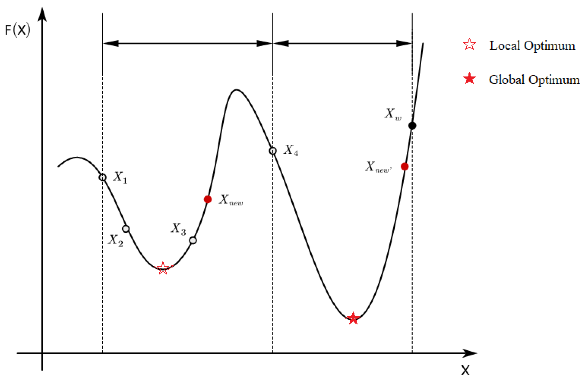
The effectiveness of BSO in solving optimization problems depends on the idea updating strategy and idea clustering method, which can generate better offspring and guide the population towards a promising area. However, Figure 1 shows that different optimization problems require different strategies to explore or exploit. Moreover, to solve a specific problem, it may be better to fully consider the characteristics of the landscape where the parent idea is located and use different strategies to explore or exploit during different stages of the evolution. Figure 2 shows an example of the potential advantages of using the worst individual to generate a new individual. In Figure 2, the X-axis represents the search space, and the F(X)-axis represents the function value of the optimization problem. The black solid dot Xw indicates the worst individual in the current population. Obviously, Xw will be eliminated in the evolution process due to the greedy selection. The new individual Xnew (red solid dot) deviates from the correct evolution direction due to the loss of diversity. Therefore, the population is easy to cluster together in the local optimum region after continuous iterative evolution. If we make a local search around Xw before it is eliminated, then (red solid dot) will be generated. Although the fitness of is worse than that of Xnew, has the potential to be closer to the global optimal solution.
Motivated by these observations, we endeavor to propose an enhanced BSO algorithm based on modified Nelder–Mead (MNM) and elite learning mechanism. First, the Nelder–Mead method is modified and used as a local search engine to fully explore more promising evolutionary direction, which can improve the exploration ability of the population. Next, the elite learning mechanism is used to enhance the exploitation ability for the evolution of the population. Finally, when the population is stagnant, the opposition learning strategy is employed to re-initialize the parent individual, which can make the population diverge into large search area and increase possibility to jump out of the local optimum.
3.2. BSONME Optimization Algorithm
3.2.1. Modified Nelder–Mead Updating Strategy
In order to enhance the local exploration ability of the population, the modified Nelder–Mead updating strategy is used to generate a new individual. For an individual Xi, the process of generating a new individual XNM is as follows. Firstly, the individuals are assumed to be organized on a ring topology in connection with their indices. The ith neighborhood includes n + 1 individuals, which is illustrated in Figure 3.
Then, the n + 1 individuals are sorted in ascending order according to their fitness values. denotes the centroid of the ith neighborhood. Xbest and Xw denote the best individual and the worst individual in the ith neighborhood, respectively. Next, the reflection transformation is used to generate a reflection individual Xnewr according to the following equation. α is set to 2.
If the fitness of the reflection individual Xnewr is worse than that of X1, Xnewr is extended in the same direction by using the expansion transformation. The expansion individual Xnewe is generated as follow.
If the fitness of the reflection individual Xnewr is worse than that of all individuals in the neighborhood, the outside contraction individual Xoc or the inside contraction individual Xic is calculated as follows:
The pseudo code of modified Nelder–Mead updating strategy (NMS) is described by Algorithm 2.
| Algorithm 2 Modified Nelder–Mead updating strategy | |
| 1: | Input the individuals in ith neighborhood |
| 2: | while the termination criteria are not met do |
| 3: | Sort the individuals in ascending order according to fitness |
| 4: | Generate a reflection individual Xnewr according to Equation (10) |
| 5: | if f(Xnewr) < f(Xbest) then |
| 6: | Generate an expansion individual Xnewe according to Equation (12) |
| 7: | if f(Xnewe) < f(Xnewr) then |
| 8: | Xw ← Xnewe; f(Xw) ← f(Xnewe) |
| 9: | else |
| 10: | Xw ← Xnewr; f(Xw) ← f(Xnewr) |
| 11: | end if |
| 12: | else |
| 13: | if f(Xnewr) < f(Xw) then |
| 14: | Xw ← Xnewr; f(Xw) ← f(Xnewr) |
| 15: | else |
| 16: | if rand < 0.5 then |
| 17: | Generate an outside contraction individual Xoc according to Equation (13) |
| 18: | if f(Xoc) < f(Xw) then |
| 19: | Xw ← Xoc; f(Xw) ← f(Xoc) |
| 20: | end if |
| 21: | else |
| 22: | Generate an inside contraction individual Xic according to Equation (14) |
| 23: | if f(Xic) < f(Xw) then |
| 24: | Xw ← Xic; f(Xw) ← f(Xic) |
| 25: | end if |
| 26: | end if |
| 27: | end if |
| 28: | end if |
| 29: | end whlie |
| 30: | Sort the individuals in ascending order according to fintness |
| 31: | Return Xbest and f(Xbest) |
3.2.2. Elite Learning Mechanism
The individuals learn from the elite individual, which may lead to a fast converging of the algorithm. A typical case is the role of gbest, the historically best position of the population, used in PSO algorithm. However, for multimodal problems, if the gbest is a local optimum, the algorithm is easy to fall into premature convergence.
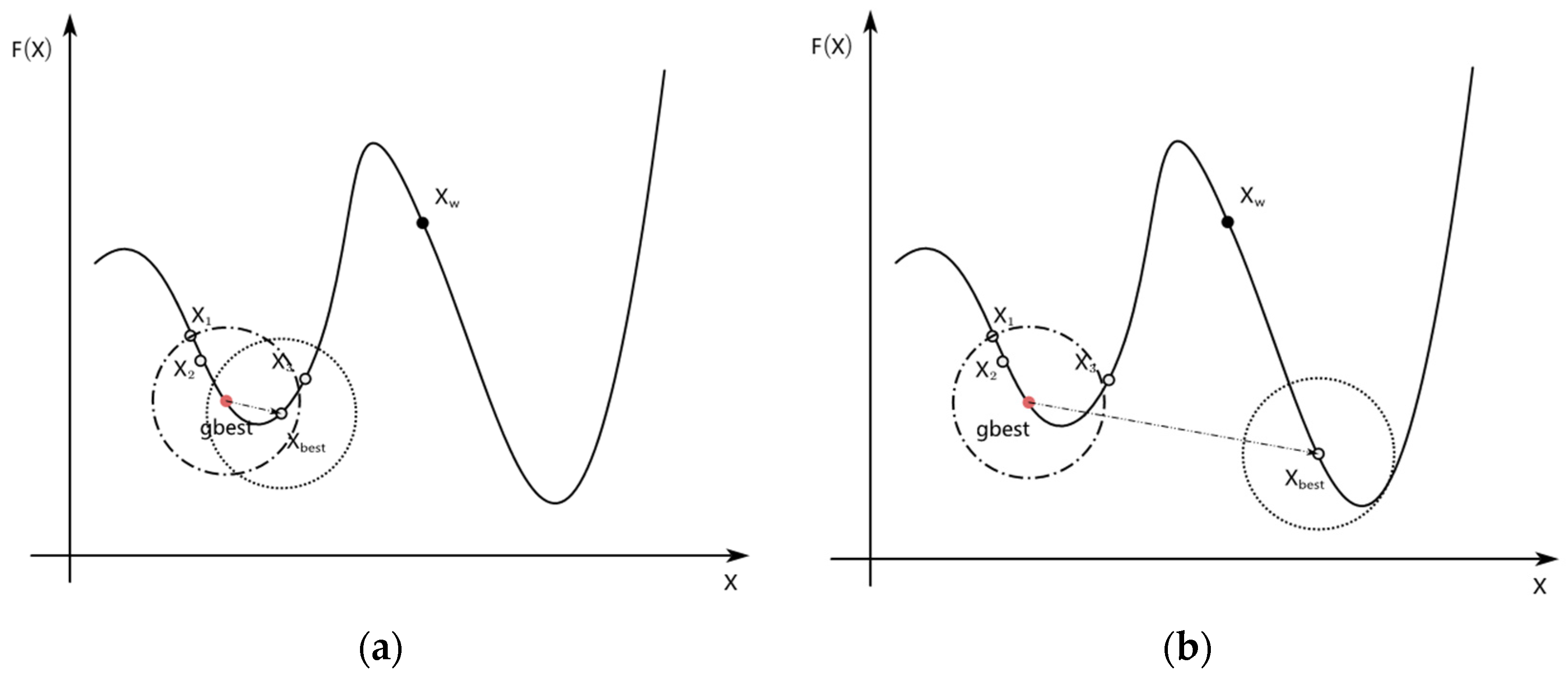
Figure 4 shows that the distance between Xbest and gbest will significantly affect the result of updating gbest. As illustrated in Figure 4, gbest (red dot) is the historical optimal solution stored in the archive. Xbest is a newly generated solution with better fitness than gbest. In Figure 4a, if gbest is updated by Xbest, the algorithm will fall into local optimization with great probability. It is advisable not to update gbest to avoid premature convergence. In Figure 4b, Xbest is far away from gbest. It is better to update gbest with Xbest to reduce the possibility of falling into local optima.
To make full use of the advantages of elite individuals and avoid premature convergence, this paper proposed an elite learning mechanism based on Euclidean distance. Here, the elite individual is denoted as gbest. In the first generation, the individual with the best fitness is selected as gbest. Figure 5 is the landscape of a two-dimensional optimization problem. Figure 6 shows the different situations for triggering the update operation. In Figure 6, gbest (the red pentagram) is the historical optimum solution. Blue squares and black triangles represent better and worse individuals, respectively. R is the average of the distance between the elite individuals and the gbest. A and B are the optimal solutions of the current generation, which may be used to update gbest. If the optimum solution A (the red quadrangle) obtained in the current generation falls into the circle, the update operation is not triggered to avoid the population falling into local optimization. On the contrary, if the optimum solution B (the red quadrangle) obtained in the current generation falls outside the circle, the update operation is triggered to guide the population to explore a more promising region.
gbest is updated as follows.
where Dis(·) is the Euclidean distance, and Xbest,t is the optimal solution at generation t; gbestt−1 is the optimal solution at generation t − 1; and Xi,t is ith individual in the elite group, which is different from Xbest,t. |elites| is the size of the elite group.
The elite learning mechanism is described as follows:
where Xselect,t is the selected individual at generate t, Xa,t and Xb,t are two randomly selected individuals, and the parameter C increases gradually in the iterative process, so as to speed up the convergence of the algorithm. The parameter is defined as follow [35].
where t and T represent the current generation and the maximum generation, respectively. Cmin and Cmax are set to 0.2 and 0.8, respectively.
3.2.3. Reinitialization Strategy
The reinitialization strategy is usually used to solve the problem of individual homogenization in the population caused by fast convergence. However, if the individual is initialized in the whole search space, the fitness of the generated individual is worse in a high probability. Then, the generated individual may easily be discarded in the evolution process. Moreover, in the later stage of evolution, the differences between individuals tend to narrow, hence, small scale disturbance on individuals cannot effectively ensure the population diversity. Research shows that opposition-based learning (OBL) can effectively accelerate the search or process because estimates and counter estimates are considered simultaneously in OBL [40]. Therefore, this paper uses OBL as the reinitialization strategy. Here, the reinitialization strategy is used according to the current convergence status. Specially, each individual is assigned a counter. If an individual is updated in each iteration, its counter is zero, otherwise its counter is incremented by 1. The reinitialization strategy is employed if the counter exceeds a given threshold.
Let X(x1, x2,…, xD) be a solution in D-dimensional space, the opposite solution of X is recorded as and is defined as follows:
where xi ∈ [ai, bi], i = 1,2, …, D.
Figure 7 illustrates the flow chart of the BSONME algorithm.
The pseudo code of BSONME is shown in Algorithm 3. The probability of random disturbance to an individual is denoted as p1. The probability of selecting the elite subpopulation is denoted as p2. The probability of selecting different strategies to generate new individuals is denoted as p3. r1 is a number randomly distributed in the range of [0, 1]. TH denotes the threshold.
| Algorithm 3 The BSONME algorithm | |
| 1: | Randomly generate N individuals |
| 2: | Evaluate N individuals |
| 3: | Randomly select an individual as gbest |
| 4: | while the termination criteria are not met do |
| 5: | Divide the population into elite population and non-elite population |
| 6: | Update gbest according to Equation (15) |
| 7: | if rand < p1 then |
| 8: | Randomly select an individual to update a selected dimension |
| 9: | end if |
| 10: | for each individual Xi do |
| 11: | if rand < p2 then |
| 12: | if rand < p3 then |
| 13: | Xselect ← Randomly select an individual from the elite subpopulation |
| 14: | else |
| 15: | Randomly select Xi and Xj from the elite subpopulation (i ≠ j) |
| 16: | Xselect = r1 × Xi + (1 − r1) × Xj |
| 17: | end if |
| 18: | else |
| 19: | if rand < p3 then |
| 20: | Xselect ← Randomly select an individual from the nonelite subpopulation |
| 21: | else |
| 22: | Randomly select Xi and Xj from the non-elite subpopulation (i ≠ j) |
| 23: | Xselect = r1 × Xi + (1 − r1) × Xj |
| 24: | end if |
| 25: | end if |
| 26: | Generate new idea Xnew according to Equation (17) |
| 27: | Evaluate Xnew |
| 28: | if f(Xnew) < f(Xi) then |
| 29: | XNMA ← perform NMS on Xi according to algorithm 2; |
| 30: | if f(XNMA) < f(Xnew) then |
| 31: | Xi ← XNMA; f(Xi) ← f(XNMA) |
| 32: | else |
| 33: | Xi ← Xnew; f(Xi) ← f(Xnew) |
| 34: | end if |
| 35: | counti = 0 |
| 36: | else |
| 37: | if counti > TH |
| 38: | Update Xi with reinitialization strategy according to Equation (19) |
| 39: | counti = 0 |
| 40: | else |
| 41: | counti = counti + 1 |
| 42: | end if |
| 43 | end if |
| 44: | end for |
| 45: | end while |
4. Comparative Studies of Experiments
In this section, experimental comparisons are made with the original algorithms and some popular BSO variants. All algorithms are tested on the CEC2014 contest benchmark problems [39] and prediction problems in the real world. The compared algorithms are listed as follows:
- Particle swarm optimization (PSO) [3];
- Brain storm optimization algorithm (BSO) [15];
- Modified brain storm optimization (MBSO) [27];
- Brain storm optimization algorithm in objective space (BSO-OS) [31];
- Random grouping brain storm optimization algorithm (RGBSO) [29];
- Improved random grouping BSO (IRGBSO) [38];
- BSO with learning strategy (BSOLS) [41];
- Active learning brain storm optimization (ALBSO) [42];
- BSO with role-playing strategy (RPBSO) [30];
- Brain storm optimization algorithm with adaptive learning strategy (BSO-AL) [34];
- Our approach (BSONME).
4.1. Parameter Settings
In this section, CEC2014 contest benchmark problems and two prediction problems are used to evaluate the performance of eleven algorithms. Details of benchmark problems and experimental setup are given in Table 2.
The performance of each algorithm is appraised by the mean value of solution error [43], which is defined in Table 1. To verify the statistical significance of the experimental results, three test measures are used, and the details of these measures are given in Table 3.
The parameter settings of different comparison algorithms are shown in Table 4.
4.2. Experiment I: Mathematical Benchmark Problems
Table 5 and Table 6 show the statistical results of 11 algorithms for solving three unimodal functions. The results show that BSONME significantly outperforms PSO, BSO, MBSO, BSO-OS, RGBSO, IRGBSO, BSOLS, ALBSO, RPBSO, and BSO-AL on 3, 3, 3, 3, 3, 3, 3, 3, 3, and 3 test problems, respectively. The proposed BSONME can beat other algorithms because the elite mechanism can guide the population move toward the more promising regions, so that the algorithm can find high-quality solutions.
In the case of F4–F16, the results show that BSONME perform the best on F8, F10, F11, and F16. BSONME outperforms PSO, BSO, MBSO, BSO-OS, RGBSO, IRGBSO, BSOLS, ALBSO, RPBSO, and BSO-AL on 5, 7, 6, 6, 7, 13, 10, 13, 7, and 12 test problems, respectively.
Table 5, Table 6, Table 7, Table 8, Table 9, Table 10, Table 11 and Table 12 show that BSONME performs well for most test problems. To further accurately evaluate the performance of each algorithm, the Wilcoxon’s test at the 5% significance level is employed based on the PR values. Table 13 shows that BSONME provides higher R + values than R − values compared with PSO, BSO, MBSO, BSO-OS, RGBSO, IRGBSO, BSOLS, ALBSO, RPBSO, and BSO-AL. The p values of PSO, BSO, MBSO, BSO-OS, RGBSO, IRGBSO, BSOLS, ALBSO, RPBSO, and BSO-AL are less than 0.05, which means that BSONME is significantly better than these competitors. Moreover, the Friedman test is utilized to rank each one according to their mean fitness. The lower the ranking of an algorithm, the better its performance. As shown in Table 14, the overall ranking sequences for the compared algorithms are BSONME, MBSO, RPBSO, BSO-OS, RGBSO, PSO, BSO, IRGBSO, BSOLS, BSO-AL, and ALBSO.
In the case of the hybrid problems F17–F22, BSONME performs better than other compared algorithms on F17, F18, and F21. BSONME wins PSO, BSO, MBSO, BSO-OS, RGBSO, IRGBSO, BSOLS, ALBSO, RPBSO, and BSO-AL on 5, 5, 2, 4, 5, 5, 6, 6, 3, and 6 test problems, respectively.
In the case of the composition problems F23–F30, the performance of BSONME is second only to that of IRGBSO. BSONME wins PSO, BSO, MBSO, BSO-OS, RGBSO, IRGBSO, BSOLS, ALBSO, RPBSO, and BSO-AL on 7, 7, 7, 8, 0, 0, 8, 8, 4, and 3 test problems, respectively.
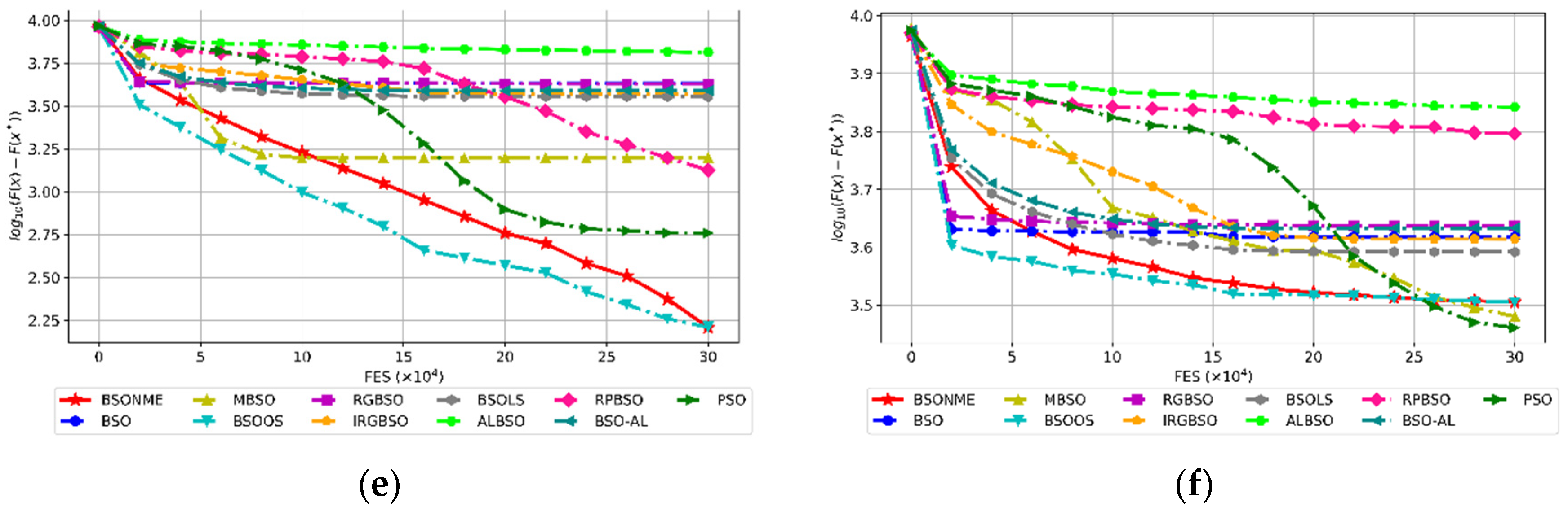
To intuitively show the convergence of each algorithm, twelve benchmark problems, including unimodal problems, multimodal problems, hybrid problems, and composite problems, are selected to plot in Figure 8 and Figure 9. In Figure 8 and Figure 9, the vertical axis is the mean errors of fitness (in logarithmic scale) and horizontal axis is the number of function evaluations. Figure 8 and Figure 9 show that BSONME converges faster than other algorithms. Moreover, BSONME performs best in terms of the lowest average best-so-far solution on most test problems.
4.3. Result and Discussion
Table 5, Table 6, Table 7, Table 8, Table 9, Table 10, Table 11 and Table 12 show that the number of “† (better)” obtained by BSONME is more than that obtained by the compared algorithms. The average excellent rate of BSONME for 30 functions is 71.67% (). The results of the multiple-problem Wilcoxon’s test and the Friedman test show that BSONME ranks first. The reason why BSONME can achieve better results is mainly due to the use of elite learning mechanism and reinitialization strategy. The elite learning mechanism helps to integrate the evolution information hidden in the superior individual into the population. The reinitialization strategy helps to improve the probability of algorithm jumping out of local optimization. We will discuss the performance of the proposed algorithm from the following three aspects.
4.3.1. Discussion on Elite Learning Mechanism and Reinitialization Strategy
To further illustrate the importance role of elite learning mechanism and reinitialization strategy, four representative problems are selected from CEC2014, including unimodal problem (F3), multimodal problem (F11), hybrid problem (F19), and composite problem (F30). In this experiment, three algorithms are compared, which are BSONME, BSO-RS (BSO with reinitialization strategy), and BSO-EL (BSO with elite learning mechanism), respectively. Figure 10 shows that the convergence performance of BSONME is better than that of BSO-RS and BSO-EL. This illustrates that elite learning mechanism and reinitialization strategy can effectively improve the performance of the algorithm.
4.3.2. Analysis of Population Diversity
Population diversity is one of the key factors affecting the exploration performance of the algorithm. In this section, the population diversity is evaluated by a moment of inertia (Ic) [46], which is defined as
where Ic denotes the spreading of each individual from their centroid. ci represents the centroid of the ith dimension, i = 1, 2, …, D.
4.3.3. The Overall Effectiveness of BSONME
This section evaluated the overall effectiveness (OE) of the BSONME and compared algorithms based on the experimental results reported in Table 5, Table 6, Table 7, Table 8, Table 9, Table 10, Table 11 and Table 12. OE is calculated as follow [47].
where N is the total number of test functions. L is the number of losing tests for each algorithm. The results are shown in Table 15. Table 15 shows that BSONME has the highest overall effectiveness, which is 60%. This shows that BSONME is an effective algorithm.
4.4. Experiment II: Least Squares Support Vector Machine for Prediction Problems
In this section, we demonstrate the efficacy of BSONME against several existing BSO optimizers and state-of-the-art methods on the real-world problem. The least squares support vector machine (LSSVM) is used to solve the prediction problems.
4.4.1. Least Squares Support Vector Machine
LSSVM is a machine learning algorithm [48] proposed by Suykens et al. LSSVM can transform the optimization problem into solving equations, and take the least square linear system as the loss function. LSSVM has been widely applied in many fields. For example, Tian et al. [49] used LSSVM to predict short-term wind speed to solve the problem of turbines optimal scheduling and ensure the safe and stable operation of power grids. Song et al. [50] established the PSO-LSSVM model, in which PSO algorithm is used to optimize the parameters of LSSVM. Then, the PSO-LSSVM model is used to predict the energy consumption of underwater gliders.
Let {(xi,yi)|i = 1, …,n} be a training set, xi is a D-dimensional input vector, and yi is output data. The optimization problem is defined as follows:
where γ > 0 is the penalty parameter, ξi is the regression error, b is the bias coefficient, and φ(x) is a nonlinear mapping function.
The Lagrange function L is constructed to solve this optimization problem.
where αi is the Lagrange multipliers.
In the paper, RBF is selected as the kernel function. RBF can be expressed as follows.
where σ is the width of the core, .
The LSSVM model is described as:
4.4.2. BSONME-LSSVM Model
The hyperparameters γ and σ have a great influence on the performance of LSSVM model, so how to optimize these two hyperparameters is the key problem. In this paper, we construct a BSONME-LSSVM model, in which BSONME algorithm is used to find the hyperparameters γ and σ with the smallest error measure. Here, the objective function is the mean square error function (fMSE) is calculated by:
where yi is the actual value and is the predicted value.
The flow chart of the proposed BSONME-LSSVM model is shown in Figure 12. The BSONME-LSSVM model finds the optimal hyperparameters through data preprocessing, initialization parameters and parameter optimization. Then, the LSSVM model is established with the optimal parameters, and the BSONME-LSSVM model is used to predict engineering problems.
4.4.3. Prediction of Pipeline Instantaneous Water Flow
Generally, urban and rural water consumption analysis can provide a reference for water plants to maintain the dynamic balance of the reservoir. Accurate prediction of pipeline instantaneous water flow can maintain the water level balance of the reservoir and effectively prevent the occurrence of water hammer.
In this section, the data of the first water plant in mishia Township, Payzawat County is used as the experimental data set. We extracted the 23-day instantaneous water flow data of the water plant. The instantaneous water flow mode of the water plant is recorded every 15 min, that is, 96 datapoints are recorded every day. A total of 2195 consecutive datapoints are used as experimental data set. For the selected experimental data, the former 1756 datapoints are selected to train the BSONME-LSSVM model, and the remaining 439 are used to verify the effectiveness of the model. The 12 consecutive units of time data are used to predict 1 unit of time data. The population size is set as 20; the ended condition of each algorithm is determined by the maximum number of iterations (MaxGen = 20). The results are shown in Table 16 in terms of Mean (mean value) and SD (standard deviation) of MSE (mean square error) obtained in the 20 independent runs for 8 optimization algorithms.
Table 16 shows that eight algorithms achieve the same results on the mean value of testing error. The mean value of training error obtained by BSONME is ranked second of eight algorithms. The standard deviation of training error and testing error obtained by BSONME is ranked third of eight algorithms.
4.4.4. Forecast of Fund Trend
Securities investment fund is a common way of investment and financial management. Accurate forecast of fund fluctuation can effectively avoid risks. Influenced by market orientation, policies, and other factors, the net value of the fund changes from time to time. Since there are many factors affecting the rise and fall of funds, in this section, in order to simplify the experiment, we only select the daily rise and fall of a fund with code 161,725 as the experimental data set (https://fund.eastmoney.com/, accessed on 13 May 2021) to predict the trend of the fund. The fund is an index stock fund with high risk. A total of 355 consecutive datapoints are used as experimental data set. For the selected experimental data, the former 284 datapoints are selected to train the BSONME-LSSVM model, and the remaining 71 are used to verify the effectiveness of the model. The five consecutive datapoints are used to predict the sixth. The population size and the ended condition of each algorithm is the same as the experimental setting in 4.4.3. The results are shown in Table 17 in terms of Mean (mean value) and SD (standard deviation) of MSE (mean square error) obtained in the 20 independent runs for 8 optimization algorithms.
Table 17 shows that eight algorithms achieve the same results on the mean value of training error. The standard deviation of training error, mean value and standard deviation of testing error obtained by BSONME is ranked first of eight algorithms. The experimental results indicate that BSONME is competitive with other seven algorithms.
5. Conclusions
In this paper, three improvement strategies are employed to improve the performance of BSO. The modified Nelder–Mead method is used as a local searcher, which fully considers the characteristics of the landscape where the parent idea located. The elite learning mechanism based on Euclidean distance is used to guide the population to move towards the promising area. Moreover, the reinitialization strategy is employed to help the population jump out of the local optimum with a large probability.
Thirty benchmark problems (CEC2014) and two engineering prediction problems (pipeline instantaneous water flow problem and fund trend problem) are used to verify the effectiveness of BSONME. The experimental results of Wilcoxon’s test and the Friedman’s test demonstrate that BSONME is competitive with some popular BSO variants in handling optimization problems. This demonstrates that the designed three improved strategies can effectively guide the population to explore and exploit, which makes the proposed algorithm achieve remarkable results.
Our future work will focus on extending BSONME to multimodal problems, multifactorial optimization problems, and multi-objective problems. Moreover, the performance of BSONME will be further improved to solve engineering problems more effectively.
Author Contributions
Conceptualization, methodology, W.L.; formal analysis, investigation, supervision, project administration, funding acquisition, W.L., H.L, Q.J. and Q.X.; resources, data curation, L.W.; writing—original draft preparation, W.L. and H.L.; writing—review and editing, L.W., Q.J. and Q.X.; All authors have read and agreed to the published version of the manuscript.
Funding
(1) National Natural Science Foundation of China under Project Code: 62176146. (2) National Natural Science Foundation of China under Project Code: 61803301. (3) National Natural Science Foundation of China under Project Code: 61773314. (4) Natural Science Basic Research Program of Shaanxi: 2020JM-709.
Institutional Review Board Statement
Not applicable.
Informed Consent Statement
Not applicable.
Data Availability Statement
Not applicable.
Conflicts of Interest
The authors declare that they have no conflicts of interest.
Appendix A
Four representative problems from CEC2014 benchmark problems mentioned in Section 3.1 are given as follows.
where o is the shifted global optimum, M is the rotation matrix, and gi(x) is ith basic function used to construct the hybrid function; , .
References
- Schranz, M.; Caro, G.; Schmickl, T.; Elmenreich, W.; Arvin, F.; Şekercioğlu, A.; Sende, M. Swarm Intelligence and Cyber-Physical Systems: Concepts, Challenges and Future Trends. Swarm Evol. Comput. 2020, 60, 100762. [Google Scholar] [CrossRef]
- Dorigo, M.; Di Caro, G. Ant colony optimization: A new meta-heuristic. In Proceedings of the IEEE Congress on Evolutionary Computation, Washington, DC, USA, 6–9 July 1999; Volume 2, pp. 1470–1477. [Google Scholar]
- Shi, Y.H.; Eberhart, R. A modified particle swarm optimizer. In Proceedings of the IEEE International Conference on Evolutionary Computation, Anchorage, AK, USA, 4–9 May 1998; pp. 611–616. [Google Scholar]
- Basturk, B.; Karaboga, D. An artifical bee colony (ABC) algorithm for numeric function optimization. In Proceedings of the IEEE Swarm Intelligence Symposium, Indianapolis, IN, USA, 12–14 May 2006; pp. 12–14. [Google Scholar]
- Simon, D. Biogeography-based optimization. IEEE Trans. Evol. Comput. 2008, 12, 702–713. [Google Scholar] [CrossRef] [Green Version]
- Gandomi, A.H.; Yang, X.S.; Alavi, A.H. Cuckoo search algorithm: A metaheuristic approach to solve structural optimization problems. Eng. Comput. 2013, 29, 17–35. [Google Scholar] [CrossRef]
- Yang, X.S. A new metaheuristic bat-inspired algorithm. In Nature Inspired Cooperative Strategies for Optimization (NICSO 2010); Springer: Berlin/Heidelberg, Germany, 2010; pp. 65–74. [Google Scholar]
- Nadimi-Shahraki, M.H.; Fatahi, A.; Zamani, H.; Mirjalili, S.; Abualigah, L. An Improved Moth-Flame Optimization Algorithm with Adaptation Mechanism to Solve Numerical and Mechanical Engineering Problems. Entropy 2021, 23, 1637. [Google Scholar] [CrossRef] [PubMed]
- Abualigah, L.; Diabat, A.; Mirjalili, S.; Abd Elaziz, M.; Gandomi, A.H. The arithmetic optimization algorithm. Comput. Methods Appl. Mech. Eng. 2021, 376, 113609. [Google Scholar] [CrossRef]
- Nadimi-Shahraki, M.H.; Fatahi, A.; Zamani, H.; Mirjalili, S.; Abualigah, L.; Abd Elaziz, M. Migration-based moth-flame opti-mization algorithm. Processes 2021, 9, 2276. [Google Scholar] [CrossRef]
- Abualigah, L.; Yousri, D.; Abd Elaziz, M.; Ewees, A.A.; Al-Qaness, M.A.; Gandomi, A.H. Aquila optimizer: A novel meta-heuristic optimization algorithm. Comput. Ind. Eng. 2021, 157, 107250. [Google Scholar] [CrossRef]
- Połap, D.; Woźniak, M. Red fox optimization algorithm. Expert Syst. Appl. 2021, 166, 114107. [Google Scholar] [CrossRef]
- Jia, H.; Peng, X.; Lang, C. Remora optimization algorithm. Expert Syst. Appl. 2021, 185, 115665. [Google Scholar] [CrossRef]
- Li, M.W.; Wang, Y.T.; Geng, J.; Hong, W.C. Chaos cloud quantum bat hybrid optimization algorithm. Nonlinear Dyn. 2021, 103, 1167–1193. [Google Scholar] [CrossRef]
- Shi, Y. Brain storm optimization algorithm. In Advances in Swarm Intelligence—Second International Conference, ICSI 2011, Chongqing, China, 12–15 June 2011; Springer: Berlin/Heidelberg, Germany, 2011; pp. 303–309. [Google Scholar]
- Papa, J.J.; Rosa, G.H.; de Souza, A.N.; Afonso, L.C.S. Feature selection through binary brain storm optimization. Comput. Electr. Eng. 2018, 72, 468–481. [Google Scholar] [CrossRef]
- Xiong, G.; Shi, D.; Zhang, J.; Zhang, Y. A binary coded brain storm optimization for fault section diagnosis of power systems. Electr. Power Syst. Res. 2018, 163, 441–451. [Google Scholar] [CrossRef]
- Pourpanah, F.; Shi, Y.; Lim, C.P.; Hao, Q.; Tan, C.J. Feature selection based on brain storm optimization for data classification. Appl. Soft Comput. J. 2019, 80, 761–775. [Google Scholar] [CrossRef]
- Wang, J.; Hou, R.; Wang, C.; Shen, L. Improved v-Support vector regression model based on variable selection and brain storm optimization for stock price forecasting. Appl. Soft Comput. 2016, 49, 164–178. [Google Scholar] [CrossRef]
- Yang, J.; Shen, Y.; Shi, Y. Visual fixation prediction with incomplete attention map based on brain storm optimization. Appl. Soft Comput. J. 2020, 96, 106653. [Google Scholar] [CrossRef]
- Duan, H.; Li, C. Quantum-behaved brain storm optimization approach to solving Loney’s solenoid problem. IEEE Trans. Magn. 2014, 51, 1–7. [Google Scholar] [CrossRef]
- Aldhafeeri, A.; Rahmat-Samii, Y. Brain storm optimization for electromagnetic applications: Continuous and discrete. IEEE Trans. Antennas Propag. 2019, 67, 2710–2722. [Google Scholar] [CrossRef]
- Jiang, Y.; Chen, X.; Zheng, F.C.; Niyato, T.D.; You, X. Brain Storm Optimization-Based Edge Caching in Fog Radio Access Networks. IEEE Trans. Veh. Technol. 2021, 70, 1807–1820. [Google Scholar] [CrossRef]
- Dai, Z.; Fang, W.; Tang, K.; Li, Q. An optima-identified framework with brain storm optimization for multimodal optimization problems. Swarm Evol. Comput. 2021, 62, 100827. [Google Scholar] [CrossRef]
- Yang, Y.; Shi, Y.; Xia, S. Advanced discussion mechanism-based brain storm optimization algorithm. Soft Comput. 2015, 19, 2997–3007. [Google Scholar] [CrossRef]
- Bezdan, T.; Stoean, C.; Naamany, A.A.; Bacanin, N.; Rashid, T.A.; Zivkovic, M.; Venkatachalam, K. Hybrid Fruit-Fly Optimization Algorithm with K-Means for Text Document Clustering. Mathematics 2021, 9, 1929. [Google Scholar] [CrossRef]
- Zhan, Z.; Zhang, J.; Shi, Y.; Liu, H. A modified brain storm optimization. In Proceedings of the 2012 IEEE Congress on Evolutionary Computation, Brisbane, Australia, 10–15 June 2012; pp. 1–8. [Google Scholar]
- Zhu, H.; Shi, Y. Brain storm optimization algorithms with k-medians clustering algorithms. In Proceedings of the 2015 Seventh International Conference on Advanced Computational Intelligence (ICACI), Wuyi, China, 27–29 March 2015; pp. 107–110. [Google Scholar]
- Cao, Z.; Shi, Y.; Rong, X.; Liu, B.; Du, Z.; Yang, B. Random grouping brain storm optimization algorithm with a new dynamically changing step size. In Proceedings of the International Conference in Swarm Intelligence, Beijing, China, 25–28 June 2015; Springer: Cham, Switzerland, 2015; pp. 357–364. [Google Scholar]
- Chen, J.; Deng, C.; Peng, H.; Tan, Y.; Wang, F. Enhanced brain storm optimization with roleplaying strategy. In Proceedings of the 2019 IEEE Congress on Evolutionary Computation (CEC), Wellington, New Zealand, 10–13 June 2019; IEEE: Pistacaway, NJ, USA, 2019; pp. 1132–1139. [Google Scholar]
- Shi, Y. Brain storm optimization algorithm in objective space. In Proceedings of the 2015 IEEE Congress on Evolutionary Computation (CEC), Sendai, Japan, 25–28 May 2015; IEEE: Pistacaway, NJ, USA, 2019; pp. 1227–1234. [Google Scholar]
- Zhou, D.; Shi, Y.; Cheng, S. Brain storm optimization algorithm with modified step-size and individual generation. In Proceedings of the International Conference in Swarm Intelligence, Shenzhen, China, 17–20 June 2012; Springer: Berlin/Heidelberg, Germany, 2012; pp. 243–252. [Google Scholar]
- Cheng, S.; Shi, Y.; Qin, Q.; Ting, T.O.; Bai, R. Maintaining population diversity in brain storm optimization algorithm. In Proceedings of the 2014 IEEE Congress on Evolutionary Computation (CEC), Beijing, China, 6–11 July 2014; pp. 3230–3237. [Google Scholar]
- Shen, Y.; Yang, J.; Cheng, S.; Shi, Y. BSO-AL: Brain storm optimization algorithm with adaptive learning strategy. In Proceedings of the 2020 IEEE Congress on Evolutionary Computation (CEC), Glasgow, UK, 19–24 July 2020; p. 17. [Google Scholar]
- El-Abd, M. Global-best brain storm optimization algorithm. Swarm Evol. Comput. 2017, 37, 27–44. [Google Scholar] [CrossRef]
- Ma, L.; Cheng, S.; Shi, Y. Enhancing learning efficiency of brain storm optimization via orthogonal learning design. IEEE Trans. Syst. Man Cybern. Syst. 2020, 51, 6723–6742. [Google Scholar] [CrossRef]
- Nelder, J.A.; Mead, R. A simplex method for function minimization. Comput. J. 1965, 7, 308–313. [Google Scholar] [CrossRef]
- El-Abd, M. Brain storm optimization algorithm with re-initialized ideas and adaptive step size. In Proceedings of the 2016 IEEE Congress on Evolutionary Computation (CEC), Vancouver, BC, Canada, 24–29 July 2016; pp. 2682–2686. [Google Scholar]
- Liang, J.J.; Qu, B.Y.; Suganthan, P.N. Problem Definitions and Evaluation Criteria for the CEC 2014 Special Session and Competition on Single Objective Real-Parameter Numerical Optimization; Computational Intelligence Laboratory, Zhengzhou University, Zhengzhou China and Technical Report; Nanyang Technological University: Singapore, 2013; Volume 635, p. 490. [Google Scholar]
- Tizhoosh, H.R. Opposition-based learning: A new scheme for machine intelligence. In Proceedings of the International Conference on Computational Intelligence for Modelling, Control and Automation and International Conference on Intelligent Agents, Web Technologies and Internet Commerce (CIMCA-IAWTIC’06), Vienna, Austria, 28–30 November 2005; Volume 1, pp. 695–701. [Google Scholar]
- Wang, H.; Liu, L.; Yi, W.; Niu, B.; Baek, J. An improved brain storm optimization with learning strategy. In Proceedings of the International Conference on Swarm Intelligence, Fukuoka, Japan, 27 July–1 August 2017; Springer: Cham, Switzerland, 2017; pp. 511–518. [Google Scholar]
- Cao, Z.; Wang, L. An active learning brain storm optimization algorithm with a dynamically changing cluster cycle for global optimization. Clust. Comput. 2019, 22, 1413–1429. [Google Scholar] [CrossRef]
- Suganthan, P.N.; Hansen, N.; Liang, J.J.; Deb, K.; Chen, Y.P.; Auger, A.; Tiwari, S. Problem Definitions and Evaluation Criteria for the CEC2005 Special Session on Real-Parameter Optimization. 2005. Available online: https://github.com/P-N-Suganthan (accessed on 13 September 2019).
- Wang, Y.; Cai, Z.; Zhang, Q. Differential evolution with composite trial vector generation strategies and control parameters. IEEE Trans. Evol. Comput. 2011, 15, 55–66. [Google Scholar] [CrossRef]
- Alcalá-Fdez, J.; Sánchez, L.; García, S.; del Jesus, M.J.; Ventura, S.; Garrell, J.M.; Otero, J.; Romero, C.; Bacardit, J.; Rivas, V.M.; et al. A software tool to assess evolutionary algorithms to data mining problems. Soft Comput. 2009, 13, 307–318. [Google Scholar] [CrossRef]
- Morrison, R.W. Designing Evolutionary Algorithms for Dynamic Environments; Springer Science & Business Media: Berlin/Heidelberg, Germany, 2004. [Google Scholar]
- Nadimi-Shahraki, M.H.; Taghian, S.; Mirjalili, S.; Faris, H. MTDE: An effective multi-trial vector-based differential evolution algorithm and its applications for engineering design problems. Appl. Soft Comput. 2020, 97, 106761. [Google Scholar] [CrossRef]
- Suykens, J.A.K.; Vandewalle, J. Least squares support vector machine classifiers. Neural Process. Lett. 1999, 9, 293–300. [Google Scholar] [CrossRef]
- Tian, Z. Short-term wind speed prediction based on LMD and improved FA optimized combined kernel function LSSVM. Eng. Appl. Artif. Intell. 2020, 91, 103573. [Google Scholar] [CrossRef]
- Song, Y.; Niu, W.; Wang, Y.; Xie, X.; Yang, S. A Novel Method for Energy Consumption Prediction of Underwater Gliders Using Optimal LSSVM with PSO Algorithm. In Proceedings of the Global Oceans 2020: Singapore—US Gulf Coast, Biloxi, MS, USA, 5–30 October 2020; pp. 1–5. [Google Scholar]
Figure 1.
Evolution of the mean errors (in logarithmic scale) of BSO, MBSO, IRGBSO, and BSO-OS versus the number of FES on four test problems. (a) F2; (b) F12; (c) F18; (d) F23.
Figure 1.
Evolution of the mean errors (in logarithmic scale) of BSO, MBSO, IRGBSO, and BSO-OS versus the number of FES on four test problems. (a) F2; (b) F12; (c) F18; (d) F23.

Figure 2.
Potential advantages of using the worst individual to generate a new individual.

Figure 3.
Ring topology of ith-neighborhood in BSONME.

Figure 4.
Different situations caused by update operation. (a) Premature convergence caused by updating gbest. (b) Jump out of local optima by updating gbest.
Figure 4.
Different situations caused by update operation. (a) Premature convergence caused by updating gbest. (b) Jump out of local optima by updating gbest.

Figure 5.
Landscape of a two-dimensional optimization problem.

Figure 6.
Different situations for triggering the update operation.

Figure 7.
Flow chart of the BSONME algorithm.

Figure 8.
Evolution of the mean values of solution error derived from PSO, BSO, MBSO, BSO-OS, RGBSO, IRGBSO, BSOLS, ALBSO, RPBSO, BSO-AL, and BSONME versus the number of FES on six test problems. (a) F1; (b) F3; (c) F4; (d) F8; (e) F10; (f) F11.
Figure 8.
Evolution of the mean values of solution error derived from PSO, BSO, MBSO, BSO-OS, RGBSO, IRGBSO, BSOLS, ALBSO, RPBSO, BSO-AL, and BSONME versus the number of FES on six test problems. (a) F1; (b) F3; (c) F4; (d) F8; (e) F10; (f) F11.


Figure 9.
Evolution of the mean values of solution error derived from PSO, BSO, MBSO, BSO-OS, RGBSO, IRGBSO, BSOLS, ALBSO, RPBSO, BSO-AL, and BSONME versus the number of FES on six test problems. (a) F16; (b) F17; (c) F18; (d) F21; (e) F27; (f) F30.
Figure 9.
Evolution of the mean values of solution error derived from PSO, BSO, MBSO, BSO-OS, RGBSO, IRGBSO, BSOLS, ALBSO, RPBSO, BSO-AL, and BSONME versus the number of FES on six test problems. (a) F16; (b) F17; (c) F18; (d) F21; (e) F27; (f) F30.

Figure 10.
Effectiveness verification of elite learning mechanism and reinitialization strategy. (a) F3; (b) F11; (c) F19; (d) F30.
Figure 10.
Effectiveness verification of elite learning mechanism and reinitialization strategy. (a) F3; (b) F11; (c) F19; (d) F30.

Figure 11.
Diversity convergence diagram of BSONME. (a) F2; (b) F5; (c) F7; (d) F9; (e) F13; (f) F17; (g) F22; (h) F26.
Figure 11.
Diversity convergence diagram of BSONME. (a) F2; (b) F5; (c) F7; (d) F9; (e) F13; (f) F17; (g) F22; (h) F26.

Figure 12.
Flow chart of the BSONME-LSSVM model.


Table 1.
Details of experimental parameters.
| Population Size | 100 |
|---|---|
| Solution Error | F(x) − F(x*) |
| F(x) | Best fitness value |
| F(x*) | Real global optimization value |
| Run times | 30 |
| Dimension (D) | 30 |
| Termination Criterion | D × 10,000 |
Table 2.
Details of CEC2014 benchmark problems and experimental setup.
| F1–F3 | Unimodal Problems |
| F4–F16 | Simple Multimodal Problems |
| F17–F22 | Hybrid Problems |
| F23–F30 | Composite Problems |
| [−100, 100]D | Search Range |
| CPU | Intel Core i7-5500 2.40 GHz |
| Application Software | Matlab R2016a |
| Termination Criterion | Maximum number of function evaluations (MaxFES) |
| MaxFES | D × 10,000 |
| Dimension | D = 30 |
| Independent run times | 30 |
| Population Size | 100 |
Table 3.
Performance measure used in the tests.
| Wilcoxon signed-rank test [44] | 5% significance level |
| Compare BSONME with other compared algorithms | |
| Multiple-problem Wilcoxon’s test [45] | Show the significant differences of the compared algorithm |
| Friedman’s test [45] | Determine the ranking of all compared algorithms |
| † | The performance of BSONME is better than that of the corresponding algorithm. |
| ≈ | The performance of BSONME is similar to that of the corresponding algorithm. |
| − | The performance of BSONME is worse than that of the corresponding algorithm. |
Table 4.
Parameter settings of compared algorithms.
| Algorithm | N | Parameter |
|---|---|---|
| PSO | 100 | c1 = 2, c2 = 2, wmax = 0.9, wmin = 0.4 |
| BSO | 100 | m = 5, preplace = 0.2, pone = 0.8, ponecenter = 0.4, ptwocenter = 0.5 |
| MBSO | 100 | m = 5, preplace = 0.2, pone = 0.8, pr = 0.005, ponecenter = 0.4, ptwocenter = 0.5 |
| BSO-OS | 100 | perce = 0.1, preplace = 0.2, pone = 0.8 |
| RGBSO | 100 | m = 5, pone = 0.8, ponecenter = 0.4, ptwocenter = 0.5 |
| IRGBSO | 100 | m = 5, pone = 0.8, ponecenter = 0.4, ptwocenter = 0.5, threshold = 10, F = 0.5 |
| BSOLS | 100 | m = 5, pone = 0.8, ponecenter = 0.4, ptwocenter = 0.5, pe = 0.1, pl = 0.1, q1 = 0.13 |
| ALBSO | 100 | m = 5, pone = 0.8, dc = 0.5, ponecenter = 0.4, ptwocenter = 0.5 |
| RPBSO | 100 | m = 3, pone = 0.5, pr = 0.005 |
| BSO-AL | 100 | m = 5, pone = 0.8, ponecenter = 0.4, ptwocenter = 0.5 |
| BSONME | 100 | p1 = 0.2, p2 = 0.2, p3 = 0.8, n = 4, TH = 50 |
Table 5.
Experimental results of PSO, BSO, MBSO, BSO-OS, RGBSO, and BSONME on F1–F3.
| F | PSO | BSO | MBSO | BSO-OS | RGBSO | BSONME |
|---|---|---|---|---|---|---|
| F1 | 7.66 × 10⁶ † | 1.75 × 10⁶ † | 5.95 × 10⁴ † | 1.69 × 10⁶ † | 2.30 × 10⁶ † | 2.76 × 10⁴ |
| F2 | 1.59 × 10² † | 8.28 × 10³ † | 14.5 † | 9.95 × 10³ † | 8.74 × 10³ † | 7.23 × 10⁻⁶ |
| F3 | 4.17 × 10² † | 1.71 × 10⁴ † | 5.23 × 10⁻¹ † | 5.71 × 10³ † | 5.47 × 10⁴ † | 8.80 × 10⁻² |
| † | 3 | 3 | 3 | 3 | 3 | \ |
| − | 0 | 0 | 0 | 0 | 0 | \ |
| ≈ | 0 | 0 | 0 | 0 | 0 | \ |
Table 6.
Experimental results of IRGBSO, BSOLS, ALBSO, RPBSO, BSO-AL, and BSONME on F1–F3.
| F | IRGBSO | BSOLS | ALBSO | RPBSO | BSO-AL | BSONME |
|---|---|---|---|---|---|---|
| F1 | 1.30 × 10⁸ † | 9.82 × 10⁶ † | 5.50 × 10⁸ † | 1.32 × 10⁶ † | 7.10 × 10⁷ † | 2.76 × 10⁴ |
| F2 | 3.49 × 10⁹ † | 1.62 × 10⁴ † | 3.31 × 10¹⁰ † | 5.73 × 10³ † | 1.04 × 10⁹ † | 7.23 × 10⁻⁶ |
| F3 | 3.17 × 10⁴ † | 2.95 × 10⁴ † | 9.83 × 10⁴ † | 1.96 × 10³ † | 8.34 × 10⁴ † | 8.80 × 10⁻² |
| † | 3 | 3 | 3 | 3 | 3 | \ |
| − | 0 | 0 | 0 | 0 | 0 | \ |
| ≈ | 0 | 0 | 0 | 0 | 0 | \ |
Table 7.
Experimental results of PSO, BSO, MBSO, BSO-OS, RGBSO, and BSONME on F4–F16.
| F | PSO | BSO | MBSO | BSO-OS | RGBSO | BSONME |
|---|---|---|---|---|---|---|
| F4 | 1.61 × 10² † | 85.8 † | 4.72 † | 65.3 † | 83.9 † | 8.06 × 10⁻¹ |
| F5 | 20.9 † | 20.0 − | 20.9 † | 20.0 − | 20.0 − | 20.1 |
| F6 | 11.0 − | 29.3 † | 3.24 − | 20.7 ≈ | 31.6 † | 20.8 |
| F7 | 1.09 × 10⁻² − | 5.26 × 10⁻⁴ − | 7.72 × 10⁻³ − | 2.49 × 10⁻³ − | 2.14 × 10⁻³ − | 4.14 × 10⁻² |
| F8 | 18.7 † | 1.39 × 10² † | 31.4 † | 12.9 † | 1.36 × 10² † | 1.63 |
| F9 | 65.3 − | 1.63 × 10² † | 36.6 − | 1.19 × 10² † | 1.79 × 10² † | 76.2 |
| F10 | 5.75 × 10² † | 4.27 × 10³ † | 1.57 × 10³ † | 1.63 × 10² † | 4.27 × 10³ † | 80.1 |
| F11 | 2.89 × 10³ ≈ | 4.15 × 10³ † | 3.02 × 10³ ≈ | 3.20 × 10³ † | 4.33 × 10³ † | 2.82 × 10³ |
| F12 | 1.78 † | 2.01 × 10⁻² − | 2.41 † | 1.66 × 10⁻² − | 4.30 × 10⁻² − | 2.62 × 10⁻¹ |
| F13 | 4.40 × 10⁻¹ ≈ | 3.33 × 10⁻¹ − | 2.49 × 10⁻¹ − | 3.14 × 10⁻¹ − | 3.54 × 10⁻¹ − | 4.77 × 10⁻¹ |
| F14 | 2.99 × 10⁻¹ ≈ | 2.18 × 10⁻¹ − | 2.85 × 10⁻¹ ≈ | 2.06 × 10⁻¹ − | 2.10 × 10⁻¹ − | 2.83 × 10⁻¹ |
| F15 | 7.87 − | 7.68 − | 2.98 − | 5.88 − | 15.3 − | 22.7 |
| F16 | 11.1 ≈ | 12.6 † | 11.6 † | 11.2 † | 12.8 † | 11.0 |
| † | 5 | 7 | 6 | 6 | 7 | \ |
| − | 4 | 6 | 5 | 6 | 6 | \ |
| ≈ | 4 | 0 | 2 | 1 | 0 | \ |
Table 8.
Experimental results of IRGBSO, BSOLS, ALBSO, RPBSO, BSO-AL, and BSONME on F4–F16.
| F | IRGBSO | BSOLS | ALBSO | RPBSO | BSO-AL | BSONME |
|---|---|---|---|---|---|---|
| F4 | 5.17 × 10² † | 61.1 † | 4.45 × 10³ † | 12.4 † | 2.12 × 10² † | 8.06 × 10⁻¹ |
| F5 | 20.3 † | 20.7 † | 21.1 † | 21.0 † | 20.7 † | 20.1 |
| F6 | 25.0 † | 34.4 † | 37.8 † | 2.77 × 10⁻¹ − | 37.9 † | 20.8 |
| F7 | 37.1 † | 1.82 × 10⁻¹ † | 3.19 × 10² † | 2.47 × 10⁻⁴ − | 5.83 † | 4.14 × 10⁻² |
| F8 | 1.80 × 10² † | 1.55 × 10² † | 2.71 × 10² † | 31.3 † | 1.58 × 10² † | 1.63 |
| F9 | 2.05 × 10² † | 1.97 × 10² † | 3.06 × 10² † | 54.7 − | 2.03 × 10² † | 76.2 |
| F10 | 3.73 × 10³ † | 3.58 × 10³ † | 6.51 × 10³ † | 1.34 × 10³ † | 3.89 × 10³ † | 80.1 |
| F11 | 4.12 × 10³ † | 3.91 × 10³ † | 6.95 × 10³ † | 6.25 × 10³ † | 4.30 × 10³ † | 2.82 × 10³ |
| F12 | 5.84 × 10⁻¹ † | 9.20 × 10⁻¹ † | 2.98 † | 2.45 † | 9.19 × 10⁻¹ † | 2.62 × 10⁻¹ |
| F13 | 8.33 × 10⁻¹ † | 4.79 × 10⁻¹ ≈ | 5.17 † | 3.46 × 10⁻¹ − | 3.84 × 10⁻¹ − | 4.77 × 10⁻¹ |
| F14 | 12.9 † | 3.32 × 10⁻¹ ≈ | 1.28 × 10² † | 2.82 × 10⁻¹ ≈ | 1.75 † | 2.83 × 10⁻¹ |
| F15 | 70.0 † | 22.2 ≈ | 1.17 × 10⁴ † | 15.3 − | 2.81 × 10⁴ † | 22.7 |
| F16 | 11.8 † | 12.3 † | 13.1 † | 12.2 † | 12.9 † | 11.0 |
| † | 13 | 10 | 13 | 7 | 12 | \ |
| − | 0 | 0 | 0 | 5 | 1 | \ |
| ≈ | 0 | 3 | 0 | 1 | 0 | \ |
Table 9.
Experimental results of PSO, BSO, MBSO, BSO-OS, RGBSO, and BSONME on F17–F22.
| F | PSO | BSO | MBSO | BSO-OS | RGBSO | BSONME |
|---|---|---|---|---|---|---|
| F17 | 6.43 × 10⁵ † | 1.21 × 10⁵ † | 8.73 × 10³ † | 8.87 × 10⁴ † | 2.05 × 10⁵ † | 4.19 × 10³ |
| F18 | 5.16 × 10³ † | 1.99 × 10³ ≈ | 3.79 × 10³ ≈ | 1.88 × 10³ ≈ | 1.60 × 10³ ≈ | 1.51 × 10³ |
| F19 | 10.1 † | 18.7 † | 5.94 − | 13.8 † | 24.8 † | 9.40 |
| F20 | 6.34 × 10² − | 1.04 × 10⁴ † | 1.51 × 10² ≈ | 1.60 × 10⁴ † | 2.42 × 10⁴ † | 2.24 × 10³ |
| F21 | 1.47 × 10⁵ † | 6.03 × 10⁴ † | 1.01 × 10⁴ † | 7.91 × 10⁴ † | 1.01 × 10⁵ † | 1.62 × 10³ |
| F22 | 2.57 × 10² − | 8.41 × 10² † | 1.61 × 10² − | 7.69 × 10² ≈ | 9.25 × 10² † | 6.67 × 10² |
| † | 4 | 5 | 2 | 4 | 5 | \ |
| − | 2 | 0 | 2 | 0 | 0 | \ |
| ≈ | 0 | 1 | 2 | 2 | 1 | \ |
Table 10.
Experimental results of IRGBSO, BSOLS, ALBSO, RPBSO, BSO-AL, and BSONME on F17–F22.
| F | IRGBSO | BSOLS | ALBSO | RPBSO | BSO-AL | BSONME |
|---|---|---|---|---|---|---|
| F17 | 2.59 × 10⁶ † | 7.29 × 10⁵ † | 3.45 × 10⁷ † | 4.03 × 10⁴ † | 7.18 × 10⁶ † | 4.19 × 10³ |
| F18 | 1.52 × 10⁶ † | 4.01 × 10³ † | 4.18 × 10⁸ † | 3.08 × 10³ ≈ | 2.66 × 10⁷ † | 1.51 × 10³ |
| F19 | 58.2 † | 21.1 † | 2.49 × 10² † | 5.13 − | 20.6 † | 9.40 |
| F20 | 2.06 × 10⁴ † | 6.82 × 10³ † | 1.10 × 10⁵ † | 2.92 × 10³ † | 1.31 × 10⁵ † | 2.24 × 10³ |
| F21 | 4.63 × 10⁵ † | 2.73 × 10⁵ † | 9.88 × 10⁶ † | 1.25 × 10⁴ † | 4.14 × 10⁶ † | 1.62 × 10³ |
| F22 | 5.50 × 10² − | 8.86 × 10² † | 1.45 × 10³ † | 64.0 − | 1.20 × 10³ † | 6.67 × 10² |
| † | 5 | 6 | 6 | 3 | 6 | \ |
| − | 1 | 0 | 0 | 2 | 0 | \ |
| ≈ | 0 | 0 | 0 | 1 | 0 | \ |
Table 11.
Experimental results of PSO, BSO, MBSO, BSO-OS, RGBSO, and BSONME on F23–F30.
| F | PSO | BSO | MBSO | BSO-OS | RGBSO | BSONME |
|---|---|---|---|---|---|---|
| F23 | 3.16 × 10² † | 3.15 × 10² † | 3.15 × 10² † | 3.14 × 10² † | 2.00 × 10² ≈ | 2.00 × 10² |
| F24 | 2.30 × 10² † | 2.51 × 10² † | 2.31 × 10² † | 2.31 × 10² † | 2.00 × 10² ≈ | 2.00 × 10² |
| F25 | 2.08 × 10² † | 2.21 × 10² † | 2.04 × 10² † | 2.18 × 10² † | 2.00 × 10² ≈ | 2.00 × 10² |
| F26 | 1.21 × 10² ≈ | 1.15 × 10² ≈ | 1.00 × 10² − | 1.73 × 10² † | 1.28 × 10² ≈ | 1.07 × 10² |
| F27 | 5.84 × 10² † | 8.44 × 10² † | 4.22 × 10² † | 7.32 × 10² † | 2.00 × 10² ≈ | 2.00 × 10² |
| F28 | 1.11 × 10³ † | 4.35 × 10³ † | 8.86 × 10² † | 3.30 × 10³ † | 2.00 × 10² ≈ | 2.00 × 10² |
| F29 | 7.92 × 10⁵ † | 3.97 × 10⁵ † | 1.34 × 10³ † | 1.48 × 10³ † | 2.00 × 10² ≈ | 2.00 × 10² |
| F30 | 4.13 × 10³ † | 8.62 × 10³ † | 1.77 × 10³ † | 3.13 × 10³ † | 2.00 × 10² ≈ | 2.00 × 10² |
| † | 7 | 7 | 7 | 8 | 0 | \ |
| − | 0 | 0 | 1 | 0 | 0 | \ |
| ≈ | 1 | 1 | 0 | 0 | 8 | \ |
Table 12.
Experimental results of IRGBSO, BSOLS, ALBSO, RPBSO, BSO-AL, and BSONME on F23–F30.
| F | IRGBSO | BSOLS | ALBSO | RPBSO | BSO-AL | BSONME |
|---|---|---|---|---|---|---|
| F23 | 2.00 × 10² ≈ | 3.20 × 10² † | 5.03 × 10² † | 2.00 × 10² ≈ | 2.00 × 10² ≈ | 2.00 × 10² |
| F24 | 2.00 × 10² ≈ | 2.58 × 10² † | 2.37 × 10² † | 2.00 × 10² † | 2.00 × 10² ≈ | 2.00 × 10² |
| F25 | 2.00 × 10² ≈ | 2.21 × 10² † | 2.17 × 10² † | 2.00 × 10² ≈ | 2.00 × 10² ≈ | 2.00 × 10² |
| F26 | 1.04 × 10² − | 1.67 × 10² † | 1.12 × 10² † | 1.10 × 10² ≈ | 1.76 × 10² † | 1.07 × 10² |
| F27 | 2.00 × 10² ≈ | 1.02 × 10³ † | 1.11 × 10³ † | 2.86 × 10² † | 2.41 × 10² ≈ | 2.00 × 10² |
| F28 | 2.00 × 10² ≈ | 1.58 × 10³ † | 4.78 × 10³ † | 2.00 × 10² ≈ | 2.00 × 10² ≈ | 2.00 × 10² |
| F29 | 2.00 × 10² ≈ | 2.88 × 10² † | 3.23 × 10⁵ † | 1.64 × 10³ † | 2.19 × 10⁵ † | 2.00 × 10² |
| F30 | 2.00 × 10² ≈ | 1.21 × 10⁴ † | 1.38 × 10⁶ † | 9.72 × 10² † | 3.21 × 10⁵ † | 2.00 × 10² |
| † | 0 | 8 | 8 | 4 | 3 | \ |
| − | 1 | 0 | 0 | 0 | 0 | \ |
| ≈ | 7 | 0 | 0 | 4 | 5 | \ |
Table 13.
Results obtained by the Wilcoxon test for algorithm BSONME.
| VS | R+ | R– | Asymptotic p-Value |
|---|---|---|---|
| PSO | 385.0 | 80.0 | 0.00165 |
| BSO | 440.0 | 25.0 | 0.000019 |
| MBSO | 350.0 | 115.0 | 0.015222 |
| BSO-OS | 433.0 | 32.0 | 0.000034 |
| RGBSO | 366.5 | 68.5 | 0.001226 |
| IRGBSO | 396.5 | 38.5 | 0.000104 |
| BSOLS | 461.0 | 4.0 | 0.000002 |
| ALBSO | 465.0 | 0.0 | 0.000002 |
| RPBSO | 367.0 | 98.0 | 0.005491 |
| BSO-AL | 455.0 | 10.0 | 0.000005 |
Table 14.
Average ranking of the algorithms (Friedman).
| Algorithm | Ranking |
|---|---|
| BSONME | 2.9333 |
| PSO | 5.65 |
| BSO | 6.1833 |
| MBSO | 3.9167 |
| BSO-OS | 4.8167 |
| RGBSO | 5.4333 |
| IRGBSO | 6.6667 |
| BSOLS | 7.7 |
| ALBSO | 10.4667 |
| RPBSO | 4.15 |
| BSO-AL | 8.0833 |
Table 15.
The overall effectiveness of the BSONME and other algorithms.
| PSO | BSO | MBSO | BSO-OS | RGBSO | IRGBSO | BSOLS | ALBSO | RPBSO | BSO-AL | BSONME | |
|---|---|---|---|---|---|---|---|---|---|---|---|
| W/T/L | 1/5/24 | 2/2/26 | 7/4/19 | 3/3/24 | 1/9/20 | 1/7/22 | 0/3/27 | 0/0/30 | 7/5/18 | 0/4/26 | 11/7/12 |
| OE | 20% | 13% | 37% | 20% | 33% | 27% | 10% | 0% | 40% | 13% | 60% |
Table 16.
Comparisons between PSO, BSO, MBSO, BSO-OS, RGBSO, IRGBSO, RPBSO, and BSONME on MSE of pipeline instantaneous water flow.
Table 16.
Comparisons between PSO, BSO, MBSO, BSO-OS, RGBSO, IRGBSO, RPBSO, and BSONME on MSE of pipeline instantaneous water flow.
| Algorithm | Training Error | Testing Error | ||
|---|---|---|---|---|
| Mean | SD | Mean | SD | |
| PSO | 6.20 | 5.89 × 10⁻³ | 5.68 | 9.08 × 10⁻⁴ |
| BSO | 6.20 | 1.27 × 10⁻² | 5.68 | 3.85 × 10⁻³ |
| MBSO | 6.20 | 3.95 × 10⁻⁴ | 5.68 | 4.39 × 10⁻⁶ |
| BSO-OS | 6.21 | 1.59 × 10⁻² | 5.68 | 6.98 × 10⁻³ |
| RGBSO | 6.19 | 2.61 × 10⁻² | 5.68 | 1.20 × 10⁻² |
| IRGBSO | 6.20 | 1.62 × 10⁻² | 5.68 | 2.54 × 10⁻³ |
| RPBSO | 6.20 | 5.80 × 10⁻⁴ | 5.68 | 6.84 × 10⁻⁶ |
| BSONME | 6.20 | 2.50 × 10⁻³ | 5.68 | 9.90 × 10⁻⁵ |
Table 17.
Comparisons between PSO, BSO, MBSO, BSO-OS, RGBSO, IRGBSO, RPBSO, and BSONME on MSE of fund trend.
Table 17.
Comparisons between PSO, BSO, MBSO, BSO-OS, RGBSO, IRGBSO, RPBSO, and BSONME on MSE of fund trend.
| Algorithm | Training Error | Testing Error | ||
|---|---|---|---|---|
| Mean | SD | Mean | SD | |
| PSO | 4.06 × 10⁻² | 2.12 × 10⁻⁵ | 3.18 × 10⁻² | 5.05 × 10⁻⁶ |
| BSO | 4.06 × 10⁻² | 5.30 × 10⁻⁵ | 3.19 × 10⁻² | 3.34 × 10⁻⁵ |
| MBSO | 4.06 × 10⁻² | 2.29 × 10⁻⁷ | 3.18 × 10⁻² | 7.51 × 10⁻⁸ |
| BSO-OS | 4.06 × 10⁻² | 7.31 × 10⁻⁵ | 3.19 × 10⁻² | 4.41 × 10⁻⁵ |
| RGBSO | 4.06 × 10⁻² | 7.70 × 10⁻⁵ | 3.19 × 10⁻² | 6.28 × 10⁻⁵ |
| IRGBSO | 4.06 × 10⁻² | 7.15 × 10⁻⁵ | 3.19 × 10⁻² | 3.62 × 10⁻⁵ |
| RPBSO | 4.06 × 10⁻² | 1.24 × 10⁻⁶ | 3.18 × 10⁻² | 5.91 × 10⁻⁷ |
| BSONME | 4.06 × 10⁻² | 1.67 × 10⁻⁷ | 3.18 × 10⁻² | 6.42 × 10⁻⁸ |
Publisher’s Note: MDPI stays neutral with regard to jurisdictional claims in published maps and institutional affiliations. |
© 2022 by the authors. Licensee MDPI, Basel, Switzerland. This article is an open access article distributed under the terms and conditions of the Creative Commons Attribution (CC BY) license (https://creativecommons.org/licenses/by/4.0/).
Share and Cite
MDPI and ACS Style
Li, W.; Luo, H.; Wang, L.; Jiang, Q.; Xu, Q. Enhanced Brain Storm Optimization Algorithm Based on Modified Nelder–Mead and Elite Learning Mechanism. Mathematics 2022, 10, 1303. https://0-doi-org.brum.beds.ac.uk/10.3390/math10081303
AMA Style
Li W, Luo H, Wang L, Jiang Q, Xu Q. Enhanced Brain Storm Optimization Algorithm Based on Modified Nelder–Mead and Elite Learning Mechanism. Mathematics. 2022; 10(8):1303. https://0-doi-org.brum.beds.ac.uk/10.3390/math10081303
Chicago/Turabian StyleLi, Wei, Haonan Luo, Lei Wang, Qiaoyong Jiang, and Qingzheng Xu. 2022. "Enhanced Brain Storm Optimization Algorithm Based on Modified Nelder–Mead and Elite Learning Mechanism" Mathematics 10, no. 8: 1303. https://0-doi-org.brum.beds.ac.uk/10.3390/math10081303
Note that from the first issue of 2016, this journal uses article numbers instead of page numbers. See further details here.