
Explainable Machine Learning Methods for Classification of Brain States during Visual Perception


1
Laboratory of Neuroscience and Cognitive Technology, Innopolis University, 1 Universitetskaya Str., 420500 Innopolis, Russia
2
Baltic Center of Neurotechnology and Artificial Intelligence, Immanuil Kant Baltic Federal University, 14 A. Nevskogo ul., 236041 Kaliningrad, Russia
3
Department of Mechanical Engineering and Instrumentation, Engineering Academy, Peoples’ Friendship University of Russia (RUDN University), 6 Miklukho-Maklaya St., 117198 Moscow, Russia
*
Author to whom correspondence should be addressed.
Mathematics 2022, 10(15), 2819; https://0-doi-org.brum.beds.ac.uk/10.3390/math10152819
Submission received: 9 June 2022
/
Revised: 22 July 2022
/
Accepted: 5 August 2022
/
Published: 8 August 2022
(This article belongs to the Special Issue Dynamics and Bifurcations in Mathematical Neuroscience: Analysis, Modeling and Applications)
Abstract
:The aim of this work is to find a good mathematical model for the classification of brain states during visual perception with a focus on the interpretability of the results. To achieve it, we use the deep learning models with different activation functions and optimization methods for their comparison and find the best model for the considered dataset of 31 EEG channels trials. To estimate the influence of different features on the classification process and make the method more interpretable, we use the SHAP library technique. We find that the best optimization method is Adagrad and the worst one is FTRL. In addition, we find that only Adagrad works well for both linear and tangent models. The results could be useful for EEG-based brain–computer interfaces (BCIs) in part for choosing the appropriate machine learning methods and features for the correct training of the BCI intelligent system.
MSC:
68T09; 92B20; 37M101. Introduction
At present, the application of artificial intelligence methods to the analysis of biological and medical data is an important and actively researched scientific task [1,2,3]. Among the works that are actively conducted in this direction are the analysis of medical images (CT and X-rays scans, etc.) [4,5], diagnostics of the human cardiovascular system [6], genomic medicine [7], different brain activity neurovisualization methods [8,9,10], etc. Within the latter, of particular interest is the diagnosis of various brain conditions and pathologies based on neuroimaging data such as a fMRI, fNIRS, MEG, and EEG [11,12,13]. In particular, machine learning methods including deep learning have found their application to process the brain signals in broad ranges, such as mental workload, disease prediction, stroke prediction [14,15], classification of EEG/MEG signals [16,17,18], prediction of sleep stages [19,20], and finding EEG biomarkers [21,22]. In the case of applying machine learning methods to diagnose EEG/MEG features in real time, there is an opportunity to implement brain–computer interfaces for neurorehabilitation, control of human brain states and robotics [23].
One of the central points of the application of artificial intelligence methods to medical and biological tasks is the interpretability of such approaches [24,25,26,27]. This is important for the creation of various assistive medical decision support systems [28,29], when a medical professional must understand and interpret the decision obtained using artificial intelligence methods. In this regard, in neuroscience, it is of great interest to develop and analyze various approaches for the diagnosis of neuroimaging data that are interpretable. Especially important is the interpretation of those features on the basis of which we create a particular machine learning system for application in biology and medicine. In the tasks of creating brain–computer interfaces for rehabilitation, communication with neurological patients, or the control of some external device, such as manipulators or exoskeletons, the most commonly used method is electroencephalography (EEG) to record brain activity and detect its features for subsequent command generation [23].
Explainable artificial intelligence (XAI) algorithms are considered to follow the principle of explainability [30]. A concept of explainability does not have a joint definition yet, so, there is a number of interpretations [31]. One of them is that explainability in machine learning can be considered as “the collection of features of the interpretable domain, that have contributed for a given example to produce a decision (e.g., classification or regression)” [32]. So, analyzing the influence of the different features on classification process is necessary for the explainable machine learning methods.
For an EEG-based brain–computer interface (BCI), deep mastering interpretability can display how different factors contained in EEG affect the machine learning model selection. For instance, Bang at al. [33] conducted analysis in comparison sample-sensible interpretation via the layer-wise relevance propagation (LRP) approach between the two subjects and revelead the potential reasons that cause the worse overall performance of one among all of them. The LRP approach is widely utilized by Sturn et al. [34] to analyze the deep learning model designed for a motor imagery mission. They assign the elements leading to an incorrect classification of artifacts of visible interest and eye movements, which remain in the EEG channels of the occipital and frontal regions. Ozdenizci at al. [35] proposed to apply a hostile inference approach to research strong features from EEG throughout unique subjects. Through interpreting the results with the LRP approach, they confirmed that their proposed method allowed the model of consciousness on neuroscience options in electroencephalogram, while it is less affected by artifacts from bone electrodes. Cui et al. [36] used magnificence’s class activation map (CAM) method [37] to examine character classifications of single-channel EEG alerts accumulated from a sustainably using enterprise. They identified that the model had been discovered to reveal brain activity patterns, such as alpha spindles and theta bursts, in addition to features that resulted from electromyography (EMG) activities, as proof to distinguish between drowsy and alert EEG alerts. In another work, Cui et al. [38] proposed a completely unique interpretation technique through taking gain of the hidden state output through the use of the long short-term memory (LSTM) layer to interpret the CNN-LSTM version designed for driving force drowsiness recognition from single-channel EEG. The same authors currently mentioned a novel interpretation method [39] based on a combination of the CAM approach [37] and the CNN–fixation techniques [40] for a multichannel EEG sign class and discovered stable functions across distinctive subjects for the venture of driver drowsiness popularity. Using the interpretation method, they also analyzed the reasons behind a few incorrectly classified samples. Regardless of the development, it is unclear to what extent the results of the interpretation may depend and how they may reflect the model’s selections. It is also not well defined in existing works why a specific interpretive technique is chosen above the other. These studies motivate us to conduct quantitative evaluations and comparisons of these interpretive strategies to gain in-depth knowledge of models designed for classification perceptual brain states of the group of voluntaries using EEG signals.
It should be noted that the convolutional neural networks (CNNs) being one of the most popular ML methods are commonly used and demonstrate a great success in image classification, natural language processing, computer vision, etc. [41,42]. However, their application to brain signals for achieving good accuracy requires a very deep CNN, which leads to a large number of parameters and high computational costs [43,44]. At the same time, the multilayer perceptrons are widely used for classifying EEG signals and demonstrate usually high efficiency [45,46].
Earlier in our works, various approaches based on machine learning have been investigated for EEG/MEG-based classification of brain states during the perception of different visual stimuli by the subject, including ambiguous images—Necker cubes [47,48,49]. In particular, the use of features based on the physiology of brain processes has been shown to improve the efficiency of the classification of brain states corresponding to the perception of visual images [50,51]. In our previous paper [52], the influence of image contrast (on the example of the famous painting by Leonardo da Vinci “Mona Lisa”) on information processing in the brain was investigated and the coherent resonance effect and reorganization of functional connections in the brain at a certain degree of image contrast were shown by the electroencephalography data. In the present work, we used this experimental dataset to classify brain states corresponding to different degrees of contrast. We also used a similar experimental dataset with EEG data on subjects’ perception of an ambiguous Necker cube with varying degrees of contrast to compare with perception of an artistic painting.
In this paper, we apply different machine-learning methods for the classification of brain states during visual perception and focus on the interpretability of the results. To estimate the influence of different features on the classification process and make the method more interpretable, we use the SHAP’s library technique. As data, we use 31-channel EEG recordings with a 250 Hz sampling rate filtered in five frequency bands. We find that a simple deep-learning model gives 100% for almost every dataset, which indicates an overfitting problem. So, we introduce four models with different combinations of two activation functions and different optimization methods. We find that the best optimization method is adagrad and the worst one is ftril. In addition, we find that only adagrad works well for both linear and tangent models. So, the contribution of the study is the following.
- We analyze the complex EEG dataset by using machine-learning techniques and find which optimization method is suitable for our dataset;
- Apply SHAP for estimation of the influence of different features to make the ML model more interpretable;
- Find the best optimizer that works well for both linear and tangent models.
The paper is organized as follows. In Section 2, we describe the EEG datasets used for the analysis, research paradigm, mathematical models of the deep learning approach (activation functions, optimization methods and the method for feature importance estimation), and case studies with the description of the neural network’s structure. Section 3 contains the results of application of different models for the classification of image intensity. In Section 4, we compare the considered deep learning methods with each other. Finally, in Section 5, we draw the conclusions.
2. Model and Methods
2.1. Datasets Description
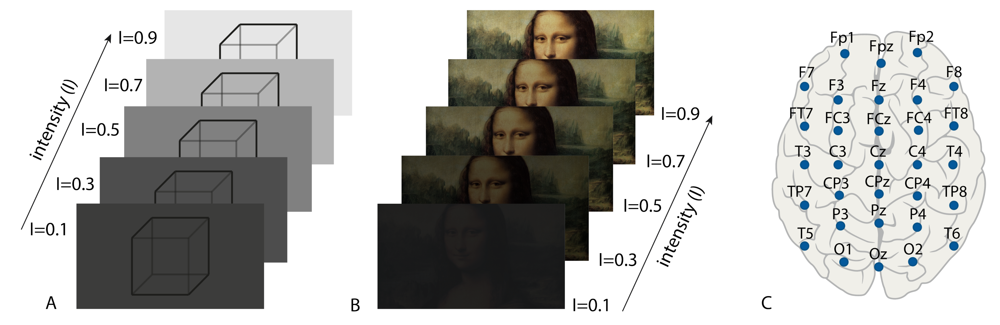
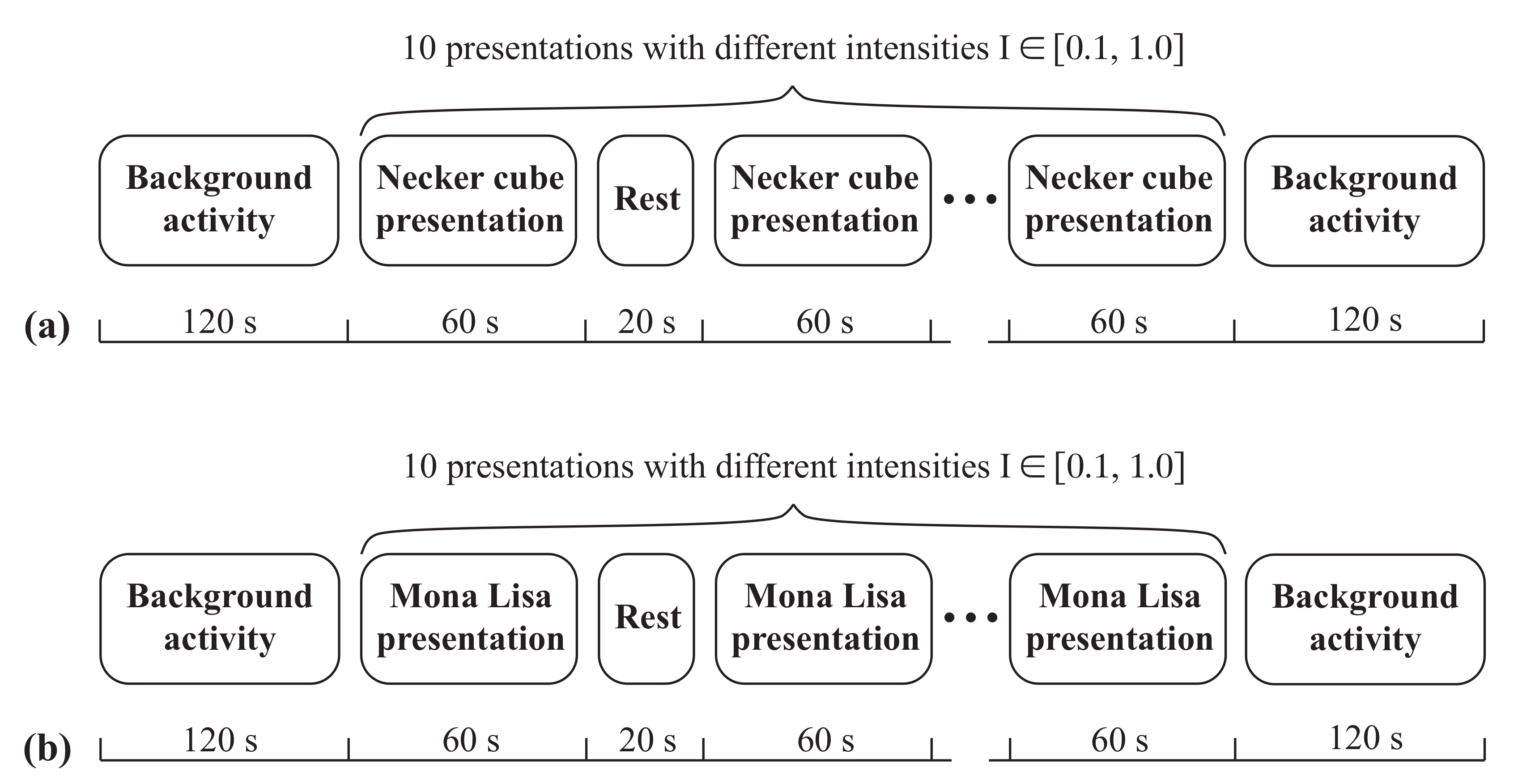
Our computational analysis is based on the experimental neurophysiological data obtained earlier in the special experiments on the visual perception of images with different contrast levels [52]. The experiment consisted of observing images of varying brightness from to , as shown in Figure 1. All the experimental EEG data of electric brain activity were recorded for 31 channels at a sampling rate of 250 Hz using the amplifier BE Plus LTM, manufactured by EB Neuro S.p.a., Florence, Italy. A detailed description of the experiment can be found in the ref. [52]. We used data from 5 subjects for two types of images. Two datasets corresponding to the observation of the ambiguous Necker cube (Figure 1A) and the Mona Lisa painting (Figure 1B) were considered. The complete set of all observed stimuli was formed by changing the brightness I of the stimuli, as shown in Figure 1A,B. A schematic illustration of the used experimental protocols is shown in Figure 2. At the start and at the end of the experiment, background activity was registered for 120 s. Each image with intensity I was presented to the subject for 60 s. Between the presentations, there was 20 s of rest. This study was conducted in accordance with the Helsinki Declaration and was approved by the Ethics Committee of Kant Baltic Federal University. All EEG data used for the analysis can be found in the repository [53].
2.2. EEG Preprocessing
Experimenters performed EEG preprocessing to remove various registration artifacts. After experimental registration, the EEG signals were filtered with a fourth-order Butterworth Hz bandpass filter and a 50 Hz notch filter. In addition, an independent component analysis (ICA) was performed to remove eye blinking and heartbeat artifacts. It should be noted that in this study, we did not conduct any experimental studies and only used previously recorded data that had already been cleared of artifacts by the above procedures and with which we did not perform any additional manipulations.
2.3. Research Paradigm
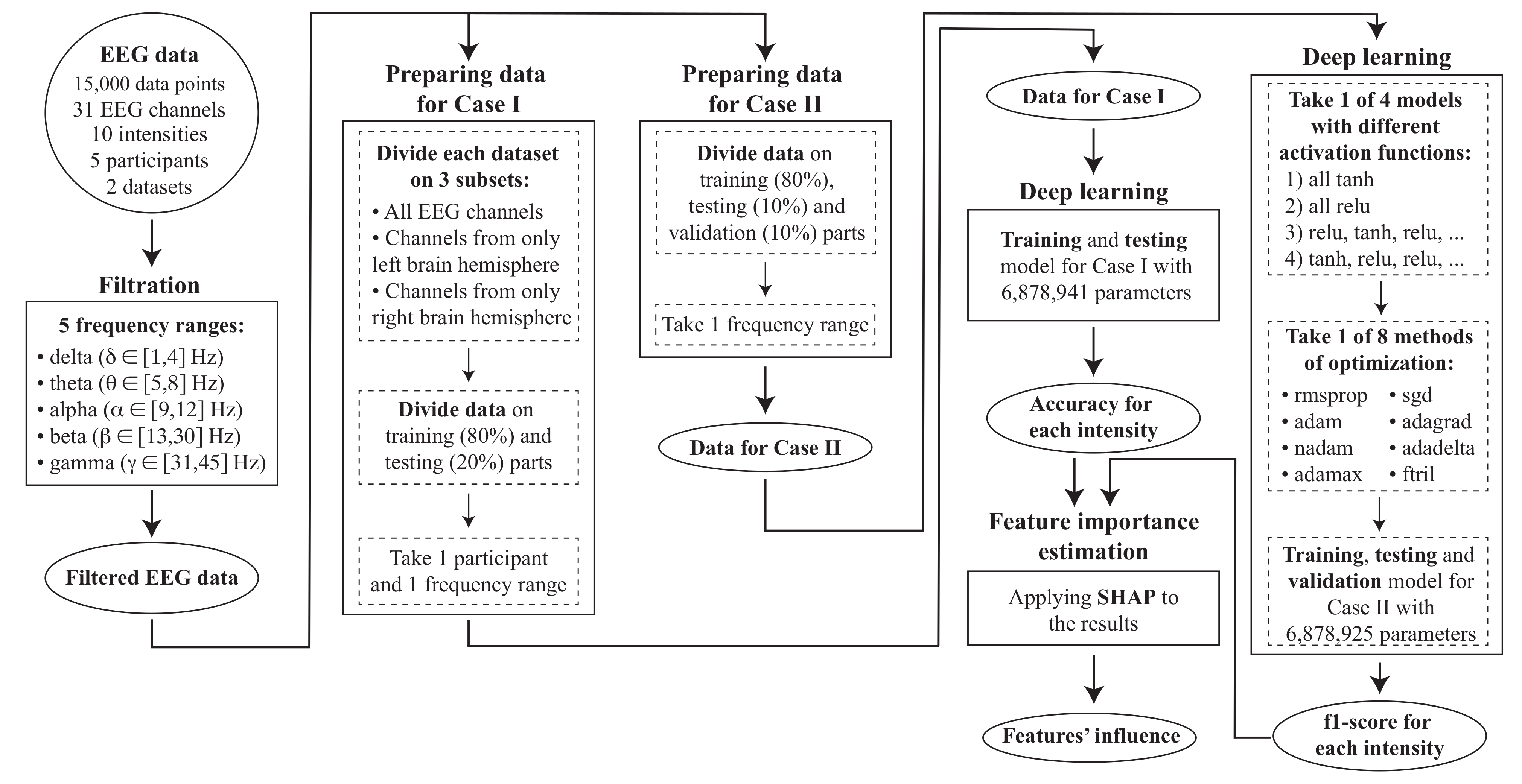
The schematic representation of the research paradigm and overall structure of the research is presented in Figure 3.
We begin our consideration with the structure of the data to be analyzed. We consider trials of the 31-channel EEG with a duration of 1 min with a sampling rate of 250 Hz for each of 10 brightnesses I, i.e., at each moment of time n for brightness I, a data vector
is registered. Here, index corresponds to EEG channels {Fp1, Fp2, …O1, O2} (see Figure 1C), is the signal registered in the i-th channel.
The most frequent and usual practice of EEG analysis is to look at different frequency ranges [54,55,56]. Here, we use the standard EEG delta-( Hz), theta-( Hz), alpha-( Hz), beta-( Hz), and gamma-( Hz) frequency ranges [57] for feature extraction and performance evaluation in perceptual brain states classification.
To obtain the data for each of the above frequency range, we reassigned the EEG signals (1) to the total average, subtracted the mean, and filtered with a fourth-order Butterworth -Hz bandpass filter, where and are the boundaries of the frequency domain of interest [58]. For example, for the -range Hz and Hz, and we obtained the alpha-band signal . Similarly, we obtain signals for all other -, -, and - frequency bands of interest.
So, we characterize the brain state during the visual perception of the images of each brightness by 60 s × 250 samples/s = 15,000 number of features (1) for each frequency band. We apply two deep learning models to classify brain states for different image brightnesses I. We consider three spatial domains of features: (i) all the EEG channels in the left and right hemispheres of the brain, (ii) EEG channels in the left hemisphere only, and (iii) EEG channels in the right hemisphere only.
We consider two separate strategies for learning and analyzing significant features that substantially affect model learning. In the first case, learning was based on the above-described features with separate frequency ranges, for each of which a different classification model was created. The input data were the trait values and image brightness I. The second case used a single model that combined all the features to predict image brightness I. In this case, different deep learning models with various neuron activation functions and various types of optimizers were used.
All deep learning models were tested on both datasets collected during the perception of images of Necker’s cube and Mona Lisa paintings. We applied SHAP (Shapley additive explanations) technology for feature importance estimation.
2.4. Mathematical Model of the Deep Learning Approach
Two types of activation functions are used: for the internal layers and for the output. For a compiler, we use as the optimizer and for loss.
The function is described as
Here, ×, where is the input layer value, is the broadcasting value through the columns (bias), is the weight value for , and L is the number of layers.
The standard function is defined as
where is the input vector, and K is the number of classes in the multi-class classifier. In our case, is the number of intensities I (Figure 1).
We also use rectified linear unit (ReLu) in the convolutions layers due to its computational simplicity and representational sparsity:
where x is the input layer value.
Next, we will describe the optimization methods we use in the paper. Here, we use the following general notation: is the model parameters we need to optimize, is the objective function, is the gradient of the objective function with respect to the parameters , is the learning rate determining the size of the steps, t is the number of step, and is a smoothing that avoids division by zero.
2.4.1. Stochastic Gradient Descent (SGD) as Optimizer
SGD is used for parameter updates for each training set. For example, if the dataset has features and target or label values, then for each step t, we have the following update rule [59]:
where .
2.4.2. Root Mean Square Propagation (RMSprop) as an Optimizer
Root Mean Square propagation (RMSprop) [59,60] is very similar to gradient descent with momentum; the only difference is that it includes the second-order momentum instead of the first-order one, plus a slight change on the parameters’ update:
where E is the decaying average over past squared gradients, and is the momentum term.
2.4.3. Adaptive Gradient Algorithm (Adagrad) as Optimizer
The adaptive gradient algorithm (Adagrad) [61] is a gradient-based optimization technique that achieves just that: it adjusts the learning rate to the parameters, producing more substantial updates for uncommon parameters and modest changes for frequent ones. As a result, it is ideal for dealing with sparse data. Dean et al. [62] discovered that Adagrad increased the robustness of SGD and used it to train large-scale neural networks at Google [63], which learned to detect cats in Youtube videos [64], among other things. In addition, Pennington et al. [65] employed Adagrad to train GloVe word embeddings, because uncommon words need considerably bigger updates than frequent words, as mentioned in Equation (7).
where is the sum of the squares of all past gradients, and ⊙ is the element-wise vector multiplication between and .
2.4.4. Extension of Adagrad (Adadelta) as Optimizer
2.4.5. Adaptive Moment Estimation (Adam) as Optimizer
Adaptive Moment Estimation (Adam) [68] is a method that can update parameters such as Adadelta and RMSprop. Here, the updated rule is as follows:
where bias-corrected moments estimate:
where and are decay rates.
2.4.6. Extension to the Adaptive Movement Estimation (AdaMax) as Optimizer
The influence in the Adam update rule scales the gradient inversely proportionally to the norm of the past gradients (via the term) and current gradient :
Then, we update to the norm with parameterization as [68]:
Norms for large p values generally become unstable. However, also generally shows balanced behavior. That is why the authors propose AdaMax [68] and show that with converges to the more stable value:
Then, we obtain the AdaMax update rule:
2.4.7. Nesterov-Accelerated Adaptive Moment Estimation (Nadam) as Optimizer
2.4.8. Follow the Regularized Leader (FTRL) as Optimizer
FTRL [70] strikes a trade-off between the advantages and disadvantages of forward–backward splitting (FBS) [71] and regularized dual averaging (RDA) [72]. The update rule is as follows:
where is the average of previous sub-gradients. In FTRL, the learning rate is different for different dimensions. If the training data deem that the dimension i needs to take a wider step than dimension j, the below learning rate will accommodate such updates:
Here, and are a non-negative and non-decreasing sequence, and is the learning rate.
2.5. SHAP (SHapley Additive exPlanations) for Feature Importance Estimation
Current explicable machine learning such as SHAP [73] supported the stochastic game [74] for a proof of model predictions. The Shapley value comes from cooperative theory of games, as an example, Shapley regression values [75] or Shapley sampling values [76]. Shapley regression values are feature importances for linear models within the presence of multiple correlation. The technique desires model fitting for all attribute subsets . Every attribute ought to receive a gain that represents its contribution to the model prediction finally. To work out this gain for a given attribute , the predictions of the 2 models are compared on the present example x, wherever denotes the values of the input options within the set . To take under consideration the influence of all alternative attributes, the variations are computed for each set . The ultimate Shapley price is calculated via a weighted average of these differences:
2.6. Case Study
We implement two case studies shown in Table 1. In the first study, we obtained the maximum accuracy, which is 100% for almost every dataset that indicates an overfitting problem. So, we introduced a second method that has a data verification step and multiple model optimizers. Here, the equations for estimating the result:
2.6.1. Case Study I
First, we implement a simple model of ANN with RMSprop optimizer (Section 2.4.2) and a structure described in Table 2. The number of connections in the input layer corresponds to the number of features (15,000), and the number of output connections is equal to the number of brightnesses (10). The number of parameters is equal to the number of connections between the layers. For example, for the input and first hidden layer, it is defined as (15,000 + 1) × 2500 = 37,502,500, where “+1” is the additional channel for the intensity. The exception is the number of the parameters for the output layer: (15 + 1) × (10 + 1) = 176. Using this model, we obtain 100% accuracy for both datasets.
2.6.2. Case Study II
Next, we use the models with verification, different activation functions and optimizers. As validation, we default to the validation built in the Keras Sequential model: we choose 10% of the original dataset as the data on which to evaluate the loss and any model metrics at the end of each epoch. The model is not trained on these data. These data are only used for tuning hyper-parameters to make the model eligible for working well on unknown data.
We consider four models, which differ from each other in activation function: tanh, relu or their combinations. The structure of the models is described in Table 3. The layers are the same as for Case I. So, the number of the parameters is also the same as for Case 1 but without an exception for the output layer: (15 + 1) × 10 = 160.
2.6.3. Computing System
The configuration of the computing system we used to perform ML follows:
• RAM: 503 GB;
• CPU: Intel(R) Xeon(R) CPU E5-2698 v4 @ 2.20 GHz;
• OS: Ubuntu 18.04.5 LTS 64 bit;
• GPU: NULL.
3. Results
In the paper, we use deep-learning neural networks with different structures, activation functions and optimizers for classification of the intensity (brightness I) of the image which was observed by the participant during the experiment. We have two datasets in which the Necker cube and Mona Lisa portrait were used as images, respectively. Each dataset includes 5 participants, 31 EEG channels, 10 intensities, and 15,000 data points for each of them. The dataset description is presented in more detail in Section 2.1.
We implement two case studies using different neural networks, which are described in Section 2.6. In both case studies, our goal is the classification of 10 intensities. Each of them is described below.
3.1. Case Study I
In this study, we decided to divide our dataset by frequency bands: , , , , and [77]. We divided our dataset into three parts based on EEG channels: (i) All channels, (ii) Channels from left hemisphere, (ii) Channels from right hemisphere, and we use the model shown in Table 2 on all of them [77]. The results of classification are shown in Table 4 and Table 5 regarding the Mona Lisa and Necker cube datasets, respectively. The results of classification for both datasets are presented in Table 4 and Table 5. Here and further, the first value for each “cell” (intersection of channels, participant and frequency band) is accuracy defined by Equation (19) (* means 100%), and the second one is the intensity which gives the maximum influence on the classification. For estimating the influence, we use SHAP (SHapley Additive exPlanations) as described in Section 2.5. In tables, we show only the intensity with maximum influence, but SHAP allows estimating the influence of all intensities I for each time point. An example is shown in Figure A1 in Appendix A.
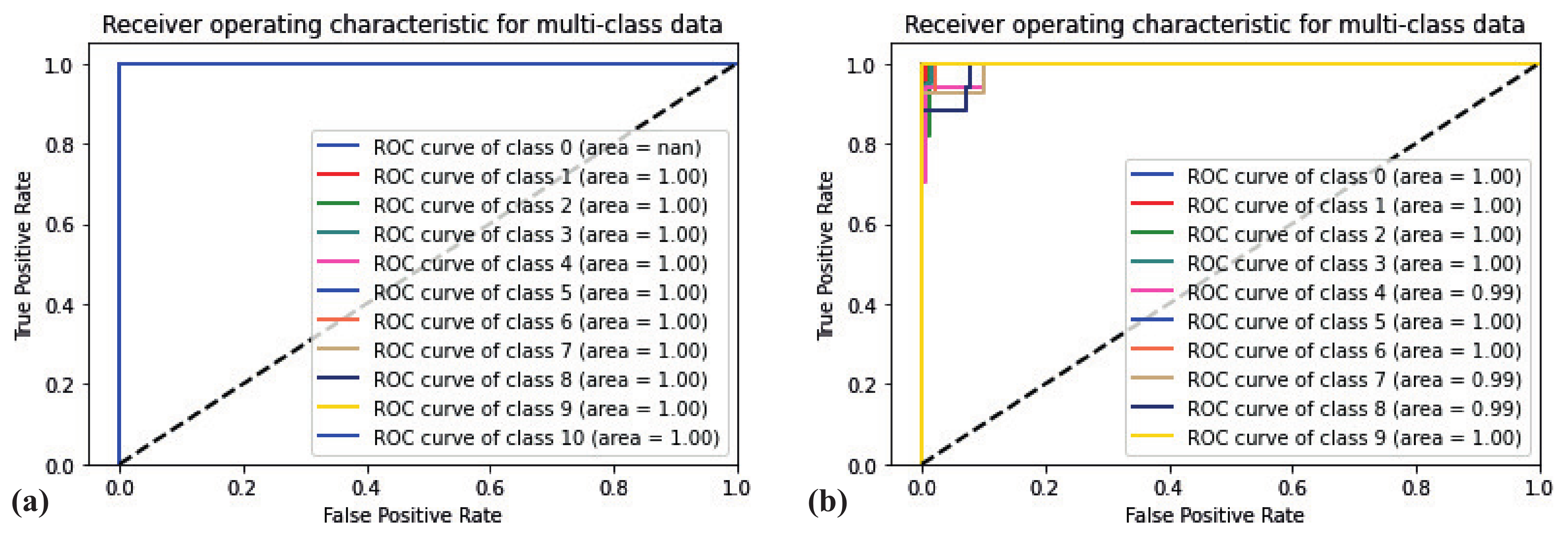
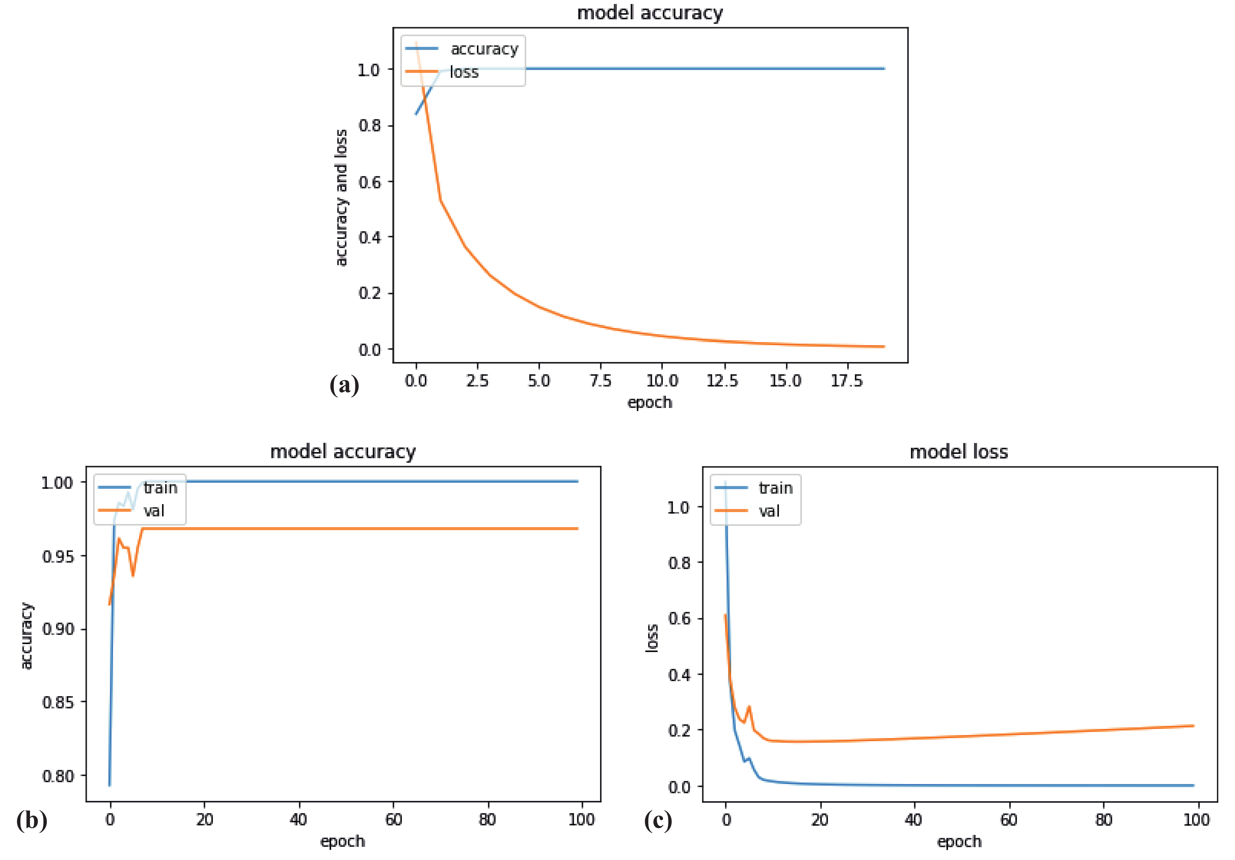
To estimate the quality of the DL model, we plot ROC, accuracy and loss curves. The ROC curves for all intensities are shown in Figure 4a. This plot is typical for every subset we investigated in Case Study I: AUC = 1.0 for every intensity, frequency range and dataset. Figure 5a illustrates the dependencies of accuracy and loss on every epoch. As one can see, the accuracy reaches 1.0 on the second epoch already, while the loss exponentially decreases with each increasing epoch.
Using this model, we obtained the maximum accuracy, which is 100% for almost every dataset that indicates an overfitting problem. So, we introduce the second method, which has a data verification step and multiple model optimizers.
The computation time for Case I is 155–162 s per model (1 dataset, 1 frequency) for all EEG channels and 74 to 82 s per model for the EEG channels from only the left or right hemisphere.
3.2. Case Study II
As it was mentioned above, using the first model for classification of the image’s intensity has an overfitting problem. To avoid it, we add data validation to our deep learning model. In addition, we estimate the f1-score (Equation (21)) instead of precision, as it was for model 1. The advantages of using the f1-score is that it can equally distribute all the classifier’s values, which cannot be done by using precision. Suppose for example that only 6 of 10 intensities were classified. Precision will work with only those 6 classified intensities, while the f1-score will use all 10 of them.
In Case Study II, we use four models (see Table 3) with different combinations of two activation functions (tanh and relu) to cross-check which model will work better (linear or tangent). We also use different optimizers to check how they perform for different models. The SHAP’s library technique [78] gives the proper explanation of the classification result of any deep learning model [77,79]. So, we can easily identify intensity with a maximum influence on classification (shown in Figure A1).
The ROC curves for all intensities are shown in Figure 4b for nadam optimizer. The curves are slightly different from the ones for Case I: not all AUCs are equal to 1.0, but all of them are higher then 0.99. As one can see, TPR is lower then 1.0 for low FPR for the number of classes, but these deviations are small and in a very short range, which indicates the high quality of the classifier. We should note that the illustrated ROC plot corresponds to the case with the highest deviation among all ROC plots. So, in every case, we have AUC ⪖ 0.99.
We estimate the accuracy and loss of the model during training and validation processes (Figure 5b,c). As one can see, the accuracy for both processes are rapidly growing and reaches its maximum value of 1.0 and 0.97, respectively, for the 10th epoch. Loss, in opposite, rapidly decreases and reaches zero value for the training process. However, for validation, it decreases up to 0.2 and then slowly increases.
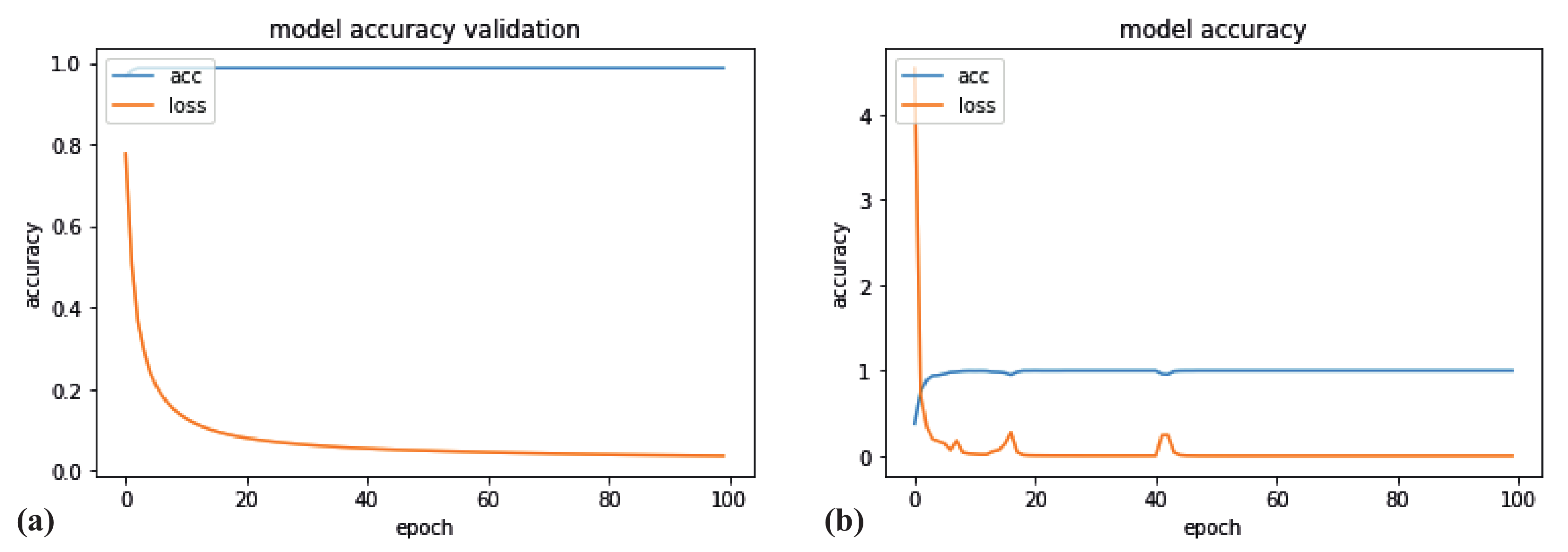
Figure 6a represents the normal dependencies of them for each epoch, which are expected to be obtained. However, in some cases, they could differ from it: instead of the accuracy being increased, it decreases for a short epoch range and returns normal after it. An example of such irregular behavior is shown in Figure 6b.
Based on that, we define five behavior activities for estimation of the applicability of the model to the dataset. The description is provided in Table 6. We compare the dependencies of accuracy and loss on the epoch to the normal ones (Figure 6a) during train and validation processes and obtain one of four results: during both processes, the dependencies correspond to the normal ones (B1), they both have irregular behavior (B2), or only one of them has irregular behavior (B3, B4). In addition, we introduce B5 behavior for the case of zero accuracy. So, B1 is the best behavior while B5 is the worst.
As it was mentioned above, in Case Study II, we use different models with different optimizers for image intensity classification by EEG signals filtered in five frequency bands. For each of them, we estimate behavior (Table 6), f1-score (Equation (21)), and the intensity with maximal influence. The computation time for Case II depends strongly on the activation function and optimization method; it varies from 288 to 6559 s per model. The average computational time for Case II is 2274 s. In the next subsections, we describe the results for each optimizer method.
3.2.1. Root Mean Square Propagation (rmsprop)
First, we use root mean square propagation (rmsprop) as the optimizer. Table 7 shows the results of application of the models with rmsprop for classification. As one can see, models 2 and 3 do not perform well since they cannot classify the intensity for three and five frequency bands, respectively, for both datasets. Other models demonstrate high accuracy (f1-score > 0.9) and excellent (B1) and good (B4) behavior. Note that most frequencies for both datasets have the same behavior for models 1 and 4.
3.2.2. Adaptive Moment Estimation (Adam)
Next, we use Adaptive Moment Estimation (adam) as an optimizer. Table 8 shows the results of application of the models with Adam for classification. As for the previous optimizer, models 2 and 3 do not perform well since they cannot classify intensity for four and five frequency bands, respectively, for both datasets. Other models demonstrate accuracy in the [0.83 0.99] range and excellent (B1) and good (B4) behavior. Note that the maximal f1-score is achieved for frequency in every dataset.
3.2.3. Nesterov-Accelerated Adaptive Moment Estimation (Nadam)
Then, we use nesterov-accelerated adaptive moment estimation (Nadam) as an optimizer. Table 9 shows the results of application the models with Nadam for classification. Again, models 2 and 3 do not perform well since they cannot classify intensity for four and five frequency bands, respectively, for both datasets. Other models demonstrate accuracy in [0.84 0.99] range as well as excellent (B1) and good (B4) behavior.
3.2.4. Extension to the Adaptive Movement Estimation (AdaMax)
The next optimizer we use is AdaMax, which is an extension to the Adaptive Movement Estimation. Table 10 shows the results of application of the models with AdaMax for classification. Comparing to all previous optimizers, AdaMax performs well for almost every frequency and model (except for model 2, which demonstrates B5 behavior for and frequencies). The accuracy for models 1, 3 and 4 are higher then 0.88. Moreover, model 1 for the Mona Lisa dataset demonstrates B1 behavior for all frequencies. The f1-score for model 4, the Mona Lisa dataset, and the frequency is 1.0. So, we need to introduce chaos [80] and dilution [81] to solve this problem for future work.
3.2.5. Adaptive Gradient Algorithm (adagrad)
Then, we use is adaptive gradient algorithm (adagrad) as optimizer. Table 11 shows the results of application the models with adagrad for classification. This algorithm does not demonstrate B5 behavior for any model. Moreover, all the models except model 2 demonstrate B1 behavior. One can see, that using lower frequency band gives higher f1-score. There are also 100% accuracy for frequency, Necker cube dataset, model 1 and 3. So, we need to introduce chaos [80] and dilution [81] to solve this problem for future work.
3.2.6. Extension of Adagrad (adadelta)
Next, we use the extension of Adagrad (Adadelta) as an optimizer. Table 12 shows the results of application of the models with Adagrad for classification. Although most models demonstrate B1 behavior, the f1-score is very low for many of them, and in some cases, it is close to zero. So, using the Adadelta optimizer does not perform good classification.
3.2.7. Stochastic Gradient Descent (SGD)
Then, we use stochastic gradient descent (SGD) as an optimizer. Table 13 shows the results of application the models with SGD for classification. With this optimizer, models 1 and 4 (start and end with tanh) work perfect for both datasets because they demonstrate B1 behavior and high accuracy for all frequencies. Model 3 has good results for almost all frequencies except one. In contrast, model 2 demonstrates B5 behavior and does not perform well.
3.2.8. Follow The Regularized Leader (FTRL)
Finally, we use the follow the regularized leader (FTRL) algorithm for optimization. As one can see from Table 14, it demonstrates B5 behavior for all the models and datasets. Only using the frequency band for model 2 gives good results.
4. Comparison of the Methods
4.1. Case Study I
As we know, right brain specialization is intuition and creativity while left brain specialization is language [82]. We found that using channels from different parts of the brain and filtering EEG signals in different frequency bands influences the classification process. Table 15 shows the intensity which gives the maximal influence on the classification process for all participants in Case Study I. As one can see, when we use all EEG channels or the ones from the right brain hemisphere, the same intensity gives the maximal influence for both datasets and all frequencies, while for left channels, the intensity differs for datasets and frequencies.
4.2. Case Study II
In Case Study II, we focus on difference keras [83] optimizers. As we mention in Table 6, we assign five behaviors. In this table, we omitted B5 behavior because it does not produce any output. The best behavior is B1, because both models have performed as a proper one. The next best one is the B3, because here, the validation performs good. The next best one will be B4, because its validation fails to perform well. So, the behavior activity from good to bad is .
Table 16 shows that the most frequent behavior of the RMSprop, Adam, Nadam, and AdaMax optimizers is B4, while for AdaMax, Adagrad, and SGD, it is B1. In our model, B1 is much better than B4. So, we can say that Adagrad is the best optimizer to use. Table 16 also gives information about which optimizer is suitable for which model. This table gives us a simple overview about linear and tangent models.
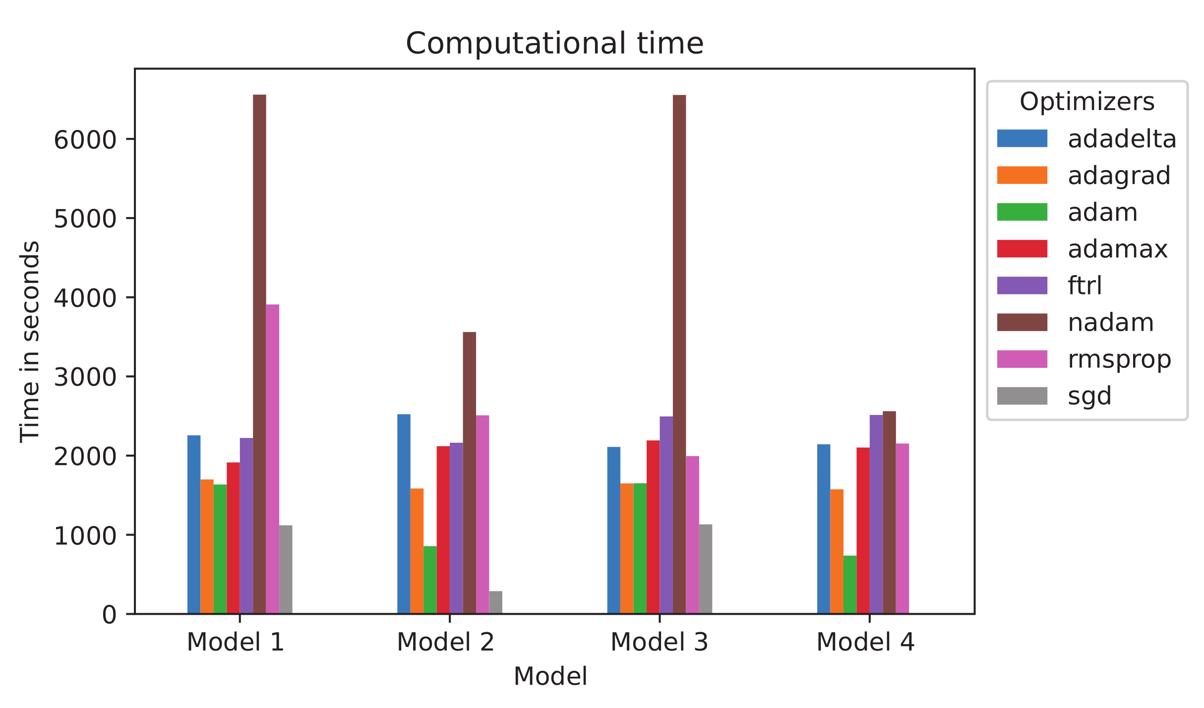
Another criterion we use for comparison of the model is the computational time (CT). Figure 7 illustrates the CT for all the models and optimizers which we have used in our research within Case Study II for frequency and the case of using all EEG channels. The lower the computational time of the machine learning method, the easier to use it. As one can see, the same optimizers marked by color require different times for the different models. The greatest difference was demonstrated by the Nadam optimization method (marked by brown color): more then 6000 s for models 1 and 3, 3500 s for model 2 and 2500 s for model 4; and RMSprop (pink): almost 4000 s for model 1 and around 2000 s for models 1, 3 and 4. The CT for Adadelta (blue), Adagrad (orange), AdaMax (red), and FTRL (violet) optimizers does not differ from one model to another. The CT for the Nadam optimizer is the highest for each model, so it is the most ineffective method among the others. In the opposite, the SGD optimization method (gray) requires the lowest CT for models 1–3, but for model 4, the most effective method is Adam (green).
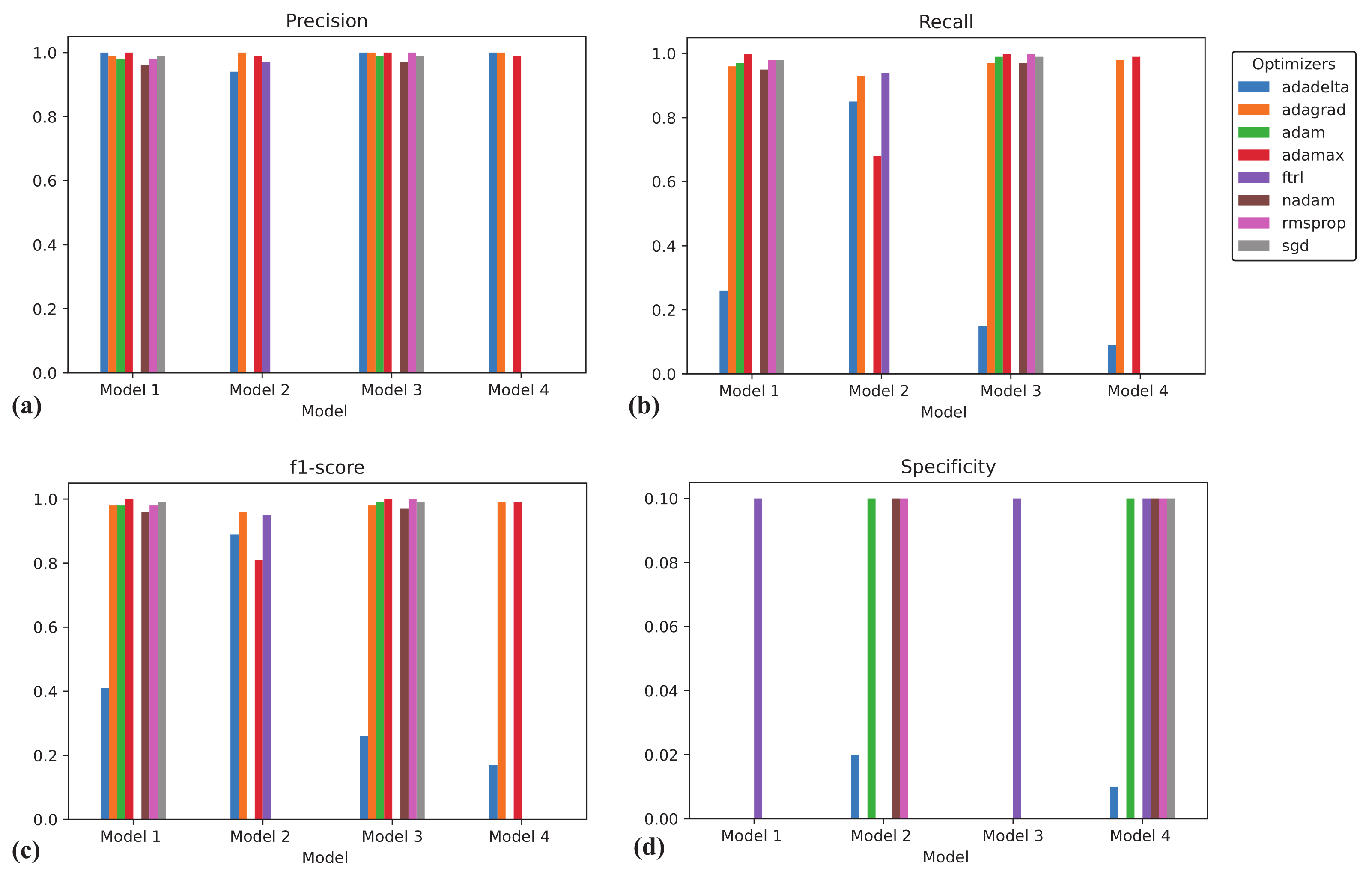
To estimate the performance of the models, we measure precision, recall, f1-score, and specificity. Figure 8 illustrates the measures for all the models and optimizers. A good model should demonstrate precision, recall and f1-score values close to 1 and specificity value close to 0. As one can see, all optimizers except FTRL have 0 specificity and very high precision for model 1 and 3, and also all except FTRL and Adadelta have high recall and f1-score for those models. So, based on these measures, we can conclude that models 1 and 3 with Adagrad, Adam, AdaMax, Nadam, RMSprop, and SGD optimization functions are better than the others.
Table 17 demonstrates a comparative study of methodologies and results between the current work and previous machine learning-based EEG studies aimed at classifying brain states In [84], the classical SVM classifier was used to classify EEG involving biological categories and non-biological categories, and it reached the classification accuracy of 82.7%. In [85], the RNN-based model was used for the classification of EEG data evoked by visual object stimuli, and 84% accuracy was achieved. In [86], the authors reached a great 96.94% f1-score, but we cannot it as the baseline since they used not only EEG signals for classification but also the original images. In our study, we use only EEG signals, and 31 channels is enough to achieve a 92.9% f1-score (average value for Model 1 over all frequencies) for the Adagrad optimizer. We should note the EEG-Net model presented in Ref. [87] where the authors used only 14 EEG channels to achieve 88% accuracy, which is a little bit less than our result. Overall, our model demonstrates a good ability to classify the EEG signals.
5. Conclusions
We have applied different machine-learning methods for the classification of brain states during visual perception. As data, we used 31 EEG channels filtered in , , , , and frequency bands corresponding to the perception of Mona Lisa and Necker cube images. In Case Study I, we used a deep learning model with eight layers, the tanh activation function, and the RMSprop optimizer. Using this model, we obtained the maximum accuracy which is 100% for almost every dataset that indicates an overfitting problem. To estimate the influence of different features on the classification process and make the method more interpretable, we use the SHAP’s library technique.
To avoid the overfitting problem of the first model, we introduced the second method (Case Study II), which has a data verification step. Here, we used four models with different combinations of two activation functions (tanh and relu) to cross-check which model works better (linear or tangent). We also used different optimizers to check how they perform for different models. We found that the best optimization method is Adagrad; it performs well for most of the frequency bands. In contrast, the FTRL method does not work at all. The list of optimizers from best to worst is: Adagrad > SGD > AdaMax > Adadelta > Nadam > RMSprop > Adam > FTRL. In addition, we found that only Adagrad works well for both linear and tangent models.
Author Contributions
Conceptualization, A.E.H.; Data curation, A.V.A. and N.N.S.; Formal analysis, R.I. and A.V.A.; Funding acquisition, N.N.S. and A.E.H.; Investigation, R.I.; Project administration, A.E.H.; Resources, N.N.S.; Software, R.I.; Supervision, A.E.H.; Validation, A.E.H.; Visualization, A.V.A.; Writing—original draft, R.I.; Writing—review and editing, A.V.A. and A.E.H. All authors have read and agreed to the published version of the manuscript.
Funding
This work has been supported by the RUDN University Strategic Academic Leadership Program.
Institutional Review Board Statement
Not applicable.
Informed Consent Statement
Not applicable.
Data Availability Statement
Dataset is available here https://drive.google.com/drive/folders/10PCSMUHLZHKRLhs-ZxKQOBBmkRTrT1Ev?usp=sharing (accessed on 8 June 2022).
Conflicts of Interest
The authors declare no conflict of interest.
Sample Availability
Code will be provided by special request.
- Case study I user based: https://colab.research.google.com/drive/1ZGDMhCc84wqiQPuyaUHpb8Q2sHqFBbOX?usp=sharing (accessed on 8 June 2022)
- Case II Mona Lisa dataset: https://drive.google.com/file/d/1qKn4wUuhouwRKH0xX2GLxxSRoR0FVVEy/view?usp=sharing (accessed on 8 June 2022)
- Case II Necker Cubes dataset: https://drive.google.com/file/d/14tsCco5P1cm3TeNXO6Zm03QH5lD6rSTM/view?usp=sharing (accessed on 8 June 2022)
Abbreviations
The following abbreviations are used in this manuscript:
| EEG | Electroencephalography |
| BCI | Brain–Computer Interface |
| Tanh | Hyperbolic Tangent |
| ReLU | Rectified Linear Unit |
| NAG | Nesterov-accelerated gradient |
| CAM | Class Activation Mapping |
| RMSprop | Root Mean Square Propagation |
| Adam | Adaptive Moment Estimation |
| Nadam | Nesterov-accelerated Adaptive Moment Estimation |
| AdaMax | Extension to the Adaptive Movement Estimation |
| Adagrad | Adaptive gradient algorithm |
| Adadelta | extension of Adagrad |
| SGD | Stochastic gradient descent |
| FTRL | Follow The Regularized Leader |
| CNN | Convolutional Neural Network |
| LRP | Layer-wise Relevance Propagation |
| FBS | Forward-Backward Splitting |
| LSTM | Long Short-Term Memory |
| RDA | Regularized Dual Averaging |
| SHAP | SHapley Additive exPlanations |
Appendix A. Application of SHAP for Feature Importance Estimation
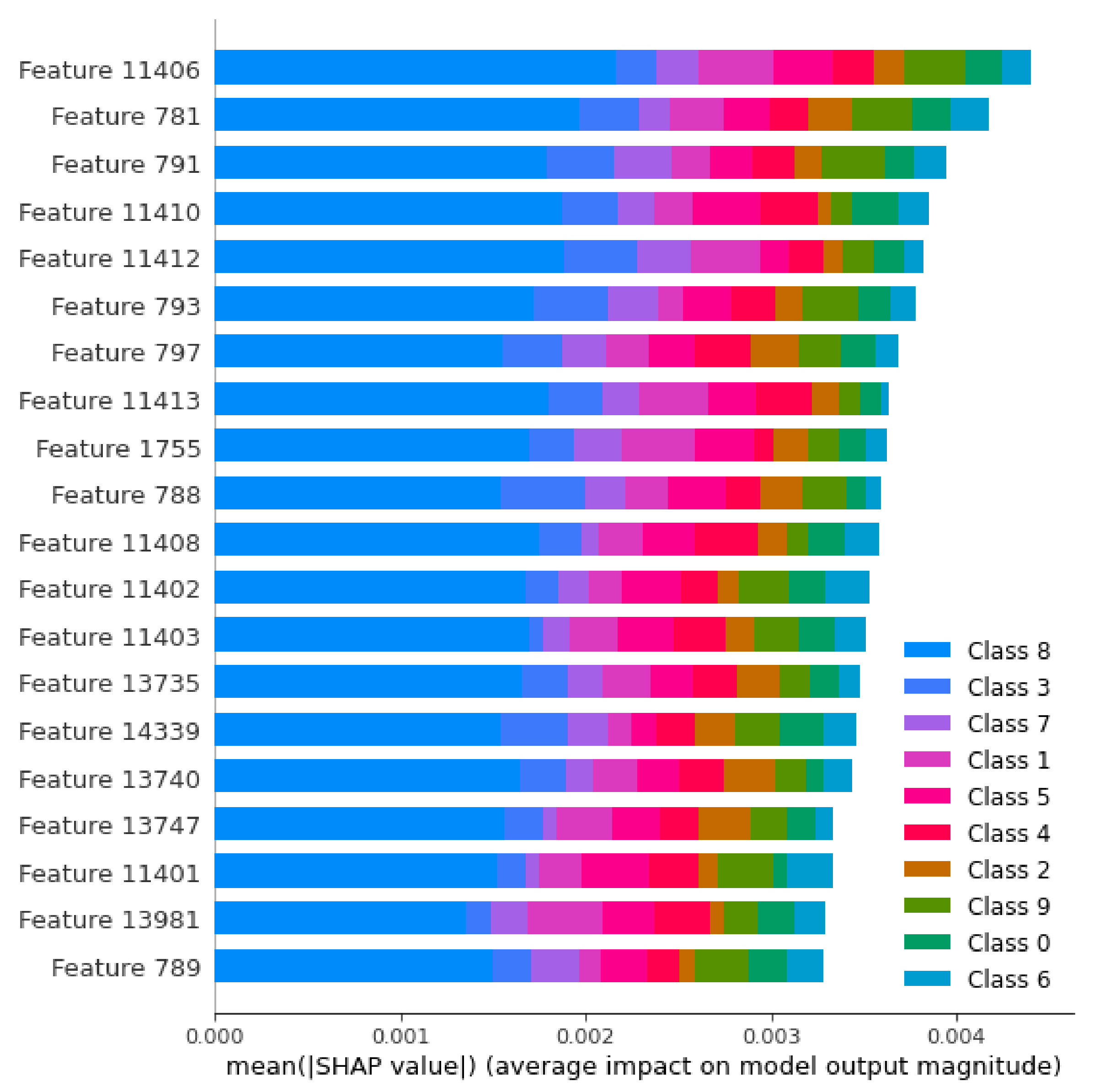
To estimate the influence of the features, we use SHAP (SHapley Additive exPlanations) as described in Section 2.5. An illustrative example of the SHAP technique application is shown in Figure A1. Here, class N corresponds to the intensity × . As one can see, feature 11,406 corresponding to 11,406/250 = 45.624 s from the beginning of image presentation has the most influence on the classification. In addition, 0.9 intensity (Class 8) influences the most for each time point.
Figure A1.
Example of top 20 features with the most influence on classification estimated by SHAP. Here, Class N corresponds to the intensity × . Feature F corresponds to the time s from the beginning of image presentation.
Figure A1.
Example of top 20 features with the most influence on classification estimated by SHAP. Here, Class N corresponds to the intensity × . Feature F corresponds to the time s from the beginning of image presentation.

References
- Yu, K.H.; Beam, A.L.; Kohane, I.S. Artificial intelligence in healthcare. Nat. Biomed. Eng. 2018, 2, 719–731. [Google Scholar] [CrossRef] [PubMed]
- He, J.; Baxter, S.L.; Xu, J.; Xu, J.; Zhou, X.; Zhang, K. The practical implementation of artificial intelligence technologies in medicine. Nat. Med. 2019, 25, 30–36. [Google Scholar] [CrossRef] [PubMed]
- Chen, I.Y.; Joshi, S.; Ghassemi, M. Treating health disparities with artificial intelligence. Nat. Med. 2020, 26, 16–17. [Google Scholar] [CrossRef] [PubMed]
- Chen, L.; Gu, D.; Chen, Y.; Shao, Y.; Cao, X.; Liu, G.; Gao, Y.; Wang, Q.; Shen, D. An artificial-intelligence lung imaging analysis system (ALIAS) for population-based nodule computing in CT scans. Comput. Med. Imaging Graph. 2021, 89, 101899. [Google Scholar] [CrossRef] [PubMed]
- Hsu, T.M.H.; Schawkat, K.; Berkowitz, S.J.; Wei, J.L.; Makoyeva, A.; Legare, K.; DeCicco, C.; Paez, S.N.; Wu, J.S.; Szolovits, P.; et al. Artificial intelligence to assess body composition on routine abdominal CT scans and predict mortality in pancreatic cancer—A recipe for your local application. Eur. J. Radiol. 2021, 142, 109834. [Google Scholar] [CrossRef] [PubMed]
- Mincholé, A.; Rodriguez, B. Artificial intelligence for the electrocardiogram. Nat. Med. 2019, 25, 22–23. [Google Scholar] [CrossRef] [PubMed]
- Dias, R.; Torkamani, A. Artificial intelligence in clinical and genomic diagnostics. Genome Med. 2019, 11, 70. [Google Scholar] [CrossRef] [PubMed] [Green Version]
- Luxton, D.D. Artificial intelligence in psychological practice: Current and future applications and implications. Prof. Psychol. Res. Pract. 2014, 45, 332. [Google Scholar] [CrossRef] [Green Version]
- Kalmady, S.V.; Greiner, R.; Agrawal, R.; Shivakumar, V.; Narayanaswamy, J.C.; Brown, M.R.; Greenshaw, A.J.; Dursun, S.M.; Venkatasubramanian, G. Towards artificial intelligence in mental health by improving schizophrenia prediction with multiple brain parcellation ensemble-learning. npj Schizophr. 2019, 5, 2. [Google Scholar] [CrossRef] [PubMed] [Green Version]
- Hu, X.S.; Nascimento, T.D.; Bender, M.C.; Hall, T.; Petty, S.; O’Malley, S.; Ellwood, R.P.; Kaciroti, N.; Maslowski, E.; DaSilva, A.F.; et al. Feasibility of a real-time clinical augmented reality and artificial intelligence framework for pain detection and localization from the brain. J. Med. Internet Res. 2019, 21, e13594. [Google Scholar] [CrossRef] [PubMed]
- Lotte, F.; Congedo, M.; Lécuyer, A.; Lamarche, F.; Arnaldi, B. A review of classification algorithms for EEG-based brain–computer interfaces. J. Neural Eng. 2007, 4, R1. [Google Scholar] [CrossRef]
- Lotte, F.; Bougrain, L.; Cichocki, A.; Clerc, M.; Congedo, M.; Rakotomamonjy, A.; Yger, F. A review of classification algorithms for EEG-based brain–computer interfaces: A 10 year update. J. Neural Eng. 2018, 15, 031005. [Google Scholar] [CrossRef] [Green Version]
- Santana, C.P.; de Carvalho, E.A.; Rodrigues, I.D.; Bastos, G.S.; de Souza, A.D.; de Brito, L.L. rs-fMRI and machine learning for ASD diagnosis: A systematic review and meta-analysis. Sci. Rep. 2022, 12, 6030. [Google Scholar] [CrossRef] [PubMed]
- Hussain, I.; Park, S.J. HealthSOS: Real-time health monitoring system for stroke prognostics. IEEE Access 2020, 8, 213574–213586. [Google Scholar] [CrossRef]
- Hussain, I.; Park, S.J. Quantitative evaluation of task-induced neurological outcome after stroke. Brain Sci. 2021, 11, 900. [Google Scholar] [CrossRef]
- Craik, A.; He, Y.; Contreras-Vidal, J.L. Deep learning for electroencephalogram (EEG) classification tasks: A review. J. Neural Eng. 2019, 16, 031001. [Google Scholar] [CrossRef]
- Al-Saegh, A.; Dawwd, S.A.; Abdul-Jabbar, J.M. Deep learning for motor imagery EEG-based classification: A review. Biomed. Signal Process. Control 2021, 63, 102172. [Google Scholar] [CrossRef]
- Chholak, P.; Niso, G.; Maksimenko, V.A.; Kurkin, S.A.; Frolov, N.S.; Pitsik, E.N.; Hramov, A.E.; Pisarchik, A.N. Visual and kinesthetic modes affect motor imagery classification in untrained subjects. Sci. Rep. 2019, 9, 9838. [Google Scholar] [CrossRef] [PubMed] [Green Version]
- Sekkal, R.N.; Bereksi-Reguig, F.; Ruiz-Fernandez, D.; Dib, N.; Sekkal, S. Automatic sleep stage classification: From classical machine learning methods to deep learning. Biomed. Signal Process. Control 2022, 77, 103751. [Google Scholar] [CrossRef]
- Hussain, I.; Hossain, M.A.; Jany, R.; Bari, M.A.; Uddin, M.; Kamal, A.R.M.; Ku, Y.; Kim, J.S. Quantitative Evaluation of EEG-Biomarkers for Prediction of Sleep Stages. Sensors 2022, 22, 3079. [Google Scholar] [CrossRef]
- Simpraga, S.; Alvarez-Jimenez, R.; Mansvelder, H.D.; Van Gerven, J.; Groeneveld, G.J.; Poil, S.S.; Linkenkaer-Hansen, K. EEG machine learning for accurate detection of cholinergic intervention and Alzheimer’s disease. Sci. Rep. 2017, 7, 5775. [Google Scholar] [CrossRef] [PubMed]
- Hussain, I.; Young, S.; Kim, C.H.; Benjamin, H.C.M.; Park, S.J. Quantifying physiological biomarkers of a microwave brain stimulation device. Sensors 2021, 21, 1896. [Google Scholar] [CrossRef] [PubMed]
- Hramov, A.E.; Maksimenko, V.A.; Pisarchik, A.N. Physical principles of brain–computer interfaces and their applications for rehabilitation, robotics and control of human brain states. Phys. Rep. 2021, 918, 1–133. [Google Scholar] [CrossRef]
- Stiglic, G.; Kocbek, P.; Fijacko, N.; Zitnik, M.; Verbert, K.; Cilar, L. Interpretability of machine learning-based prediction models in healthcare. Wiley Interdiscip. Rev. Data Min. Knowl. Discov. 2020, 10, e1379. [Google Scholar] [CrossRef]
- Wang, F.; Kaushal, R.; Khullar, D. Should Health Care Demand Interpretable Artificial Intelligence or Accept “Black Box” Medicine? Ann. Intern. Med. 2020, 172, 59–60. [Google Scholar] [CrossRef] [PubMed]
- Kundu, S. AI in medicine must be explainable. Nat. Med. 2021, 27, 1328. [Google Scholar] [CrossRef] [PubMed]
- Belle, V.; Papantonis, I. Principles and practice of explainable machine learning. Front. Big Data 2021, 4, 688969. [Google Scholar] [CrossRef] [PubMed]
- Kaur, S.; Singla, J.; Nkenyereye, L.; Jha, S.; Prashar, D.; Joshi, G.P.; El-Sappagh, S.; Islam, M.S.; Islam, S.R. Medical diagnostic systems using artificial intelligence (ai) algorithms: Principles and perspectives. IEEE Access 2020, 8, 228049–228069. [Google Scholar] [CrossRef]
- Vasey, B.; Clifton, D.A.; Collins, G.S.; Denniston, A.K.; Faes, L.; Geerts, B.F.; Liu, X.; Morgan, L.; Watkinson, P.; McCulloch, P.; et al. DECIDE-AI: New reporting guidelines to bridge the development-to-implementation gap in clinical artificial intelligence. Nat. Med. 2021, 27, 186–187. [Google Scholar]
- Adadi, A.; Berrada, M. Peeking inside the black-box: A survey on explainable artificial intelligence (XAI). IEEE Access 2018, 6, 52138–52160. [Google Scholar] [CrossRef]
- Roscher, R.; Bohn, B.; Duarte, M.F.; Garcke, J. Explainable machine learning for scientific insights and discoveries. IEEE Access 2020, 8, 42200–42216. [Google Scholar] [CrossRef]
- Montavon, G.; Samek, W.; Müller, K.R. Methods for interpreting and understanding deep neural networks. Digit. Signal Process. 2018, 73, 1–15. [Google Scholar] [CrossRef]
- Bang, J.S.; Lee, M.H.; Fazli, S.; Guan, C.; Lee, S.W. Spatio-spectral feature representation for motor imagery classification using convolutional neural networks. IEEE Trans. Neural Netw. Learn. Syst. 2021, 33, 3038–3049. [Google Scholar] [CrossRef]
- Sturm, I.; Lapuschkin, S.; Samek, W.; Müller, K.R. Interpretable deep neural networks for single-trial EEG classification. J. Neurosci. Methods 2016, 274, 141–145. [Google Scholar] [CrossRef] [PubMed] [Green Version]
- Özdenizci, O.; Wang, Y.; Koike-Akino, T.; Erdoğmuş, D. Learning invariant representations from EEG via adversarial inference. IEEE Access 2020, 8, 27074–27085. [Google Scholar] [CrossRef]
- Cui, J.; Lan, Z.; Liu, Y.; Li, R.; Li, F.; Sourina, O.; Müller-Wittig, W. A compact and interpretable convolutional neural network for cross-subject driver drowsiness detection from single-channel EEG. Methods 2021, 202, 173–184. [Google Scholar] [CrossRef] [PubMed]
- Zhou, B.; Khosla, A.; Lapedriza, A.; Oliva, A.; Torralba, A. Learning deep features for discriminative localization. In Proceedings of the IEEE Conference on Computer Vision and Pattern Recognition, Las Vegas, NV, USA, 27–30 June 2016; pp. 2921–2929. [Google Scholar]
- Cui, J.; Lan, Z.; Zheng, T.; Liu, Y.; Sourina, O.; Wang, L.; Müller-Wittig, W. Subject-Independent Drowsiness Recognition from Single-Channel EEG with an Interpretable CNN-LSTM model. In Proceedings of the 2021 International Conference on Cyberworlds (CW), Caen, France, 28–30 September 2021; pp. 201–208. [Google Scholar]
- Cui, J.; Lan, Z.; Sourina, O.; Müller-Wittig, W. EEG-Based Cross-Subject Driver Drowsiness Recognition With an Interpretable Convolutional Neural Network. IEEE Trans. Neural Netw. Learn. Syst. 2022. [Google Scholar] [CrossRef] [PubMed]
- Mopuri, K.R.; Garg, U.; Babu, R.V. Cnn fixations: An unraveling approach to visualize the discriminative image regions. IEEE Trans. Image Process. 2018, 28, 2116–2125. [Google Scholar] [CrossRef] [PubMed] [Green Version]
- Gu, J.; Wang, Z.; Kuen, J.; Ma, L.; Shahroudy, A.; Shuai, B.; Liu, T.; Wang, X.; Wang, G.; Cai, J.; et al. Recent advances in convolutional neural networks. Pattern Recognit. 2018, 77, 354–377. [Google Scholar] [CrossRef] [Green Version]
- Li, Z.; Liu, F.; Yang, W.; Peng, S.; Zhou, J. A survey of convolutional neural networks: Analysis, applications, and prospects. IEEE Trans. Neural Netw. Learn. Syst. 2021. [Google Scholar] [CrossRef] [PubMed]
- Xu, G.; Shen, X.; Chen, S.; Zong, Y.; Zhang, C.; Yue, H.; Liu, M.; Chen, F.; Che, W. A deep transfer convolutional neural network framework for EEG signal classification. IEEE Access 2019, 7, 112767–112776. [Google Scholar] [CrossRef]
- Jiao, Z.; Gao, X.; Wang, Y.; Li, J.; Xu, H. Deep convolutional neural networks for mental load classification based on EEG data. Pattern Recognit. 2018, 76, 582–595. [Google Scholar] [CrossRef]
- Abbasi, S.F.; Ahmad, J.; Tahir, A.; Awais, M.; Chen, C.; Irfan, M.; Siddiqa, H.A.; Waqas, A.B.; Long, X.; Yin, B.; et al. EEG-based neonatal sleep-wake classification using multilayer perceptron neural network. IEEE Access 2020, 8, 183025–183034. [Google Scholar] [CrossRef]
- Sharma, R.; Kim, M.; Gupta, A. Motor imagery classification in brain-machine interface with machine learning algorithms: Classical approach to multi-layer perceptron model. Biomed. Signal Process. Control 2022, 71, 103101. [Google Scholar] [CrossRef]
- Hramov, A.E.; Maksimenko, V.A.; Pchelintseva, S.V.; Runnova, A.E.; Grubov, V.V.; Musatov, V.Y.; Zhuravlev, M.O.; Koronovskii, A.A.; Pisarchik, A.N. Classifying the perceptual interpretations of a bistable image using EEG and artificial neural networks. Front. Neurosci. 2017, 11, 674. [Google Scholar] [CrossRef] [PubMed] [Green Version]
- Hramov, A.E.; Frolov, N.S.; Maksimenko, V.A.; Makarov, V.V.; Koronovskii, A.A.; Garcia-Prieto, J.; Antón-Toro, L.F.; Maestú, F.; Pisarchik, A.N. Artificial neural network detects human uncertainty. Chaos Interdiscip. J. Nonlinear Sci. 2018, 28, 033607. [Google Scholar] [CrossRef] [PubMed]
- Frolov, N.; Kabir, M.S.; Maksimenko, V.; Hramov, A. Machine learning evaluates changes in functional connectivity under a prolonged cognitive load. Chaos Interdiscip. J. Nonlinear Sci. 2021, 31, 101106. [Google Scholar] [CrossRef] [PubMed]
- Hramov, A.E.; Maksimenko, V.; Koronovskii, A.; Runnova, A.E.; Zhuravlev, M.; Pisarchik, A.N.; Kurths, J. Percept-related EEG classification using machine learning approach and features of functional brain connectivity. Chaos Interdiscip. J. Nonlinear Sci. 2019, 29, 093110. [Google Scholar] [CrossRef] [PubMed]
- Kuc, A.; Korchagin, S.; Maksimenko, V.A.; Shusharina, N.; Hramov, A.E. Combining Statistical Analysis and Machine Learning for EEG Scalp Topograms Classification. Front. Syst. Neurosci. 2021, 15, 716897. [Google Scholar] [CrossRef] [PubMed]
- Pisarchik, A.N.; Maksimenko, V.A.; Andreev, A.V.; Frolov, N.S.; Makarov, V.V.; Zhuravlev, M.O.; Runnova, A.E.; Hramov, A.E. Coherent resonance in the distributed cortical network during sensory information processing. Sci. Rep. 2019, 9, 18325. [Google Scholar] [CrossRef] [PubMed] [Green Version]
- Islam, R.; Hramov, A.E.; Andreev, A. EEG Data Set; Figshare: Iasi, Romania, 2022. [Google Scholar] [CrossRef]
- Blanco, S.; Quiroga, R.Q.; Rosso, O.; Kochen, S. Time-frequency analysis of electroencephalogram series. Phys. Rev. E 1995, 51, 2624. [Google Scholar] [CrossRef] [Green Version]
- Wang, Y.; Veluvolu, K.C.; Lee, M. Time-frequency analysis of band-limited EEG with BMFLC and Kalman filter for BCI applications. J. Neuroeng. Rehabil. 2013, 10, 109. [Google Scholar] [CrossRef] [Green Version]
- Herrmann, C.S.; Strüber, D.; Helfrich, R.F.; Engel, A.K. EEG oscillations: From correlation to causality. Int. J. Psychophysiol. 2016, 103, 12–21. [Google Scholar] [CrossRef] [PubMed]
- Kane, N.; Acharya, J.; Beniczky, S.; Caboclo, L.; Finnigan, S.; Kaplan, P.W.; Shibasaki, H.; Pressler, R.; van Putten, M.J. A revised glossary of terms most commonly used by clinical electroencephalographers and updated proposal for the report format of the EEG findings. Revision 2017. Clin. Neurophysiol. Pract. 2017, 2, 170. [Google Scholar] [CrossRef] [PubMed]
- Kuc, A.K.; Kurkin, S.A.; Maksimenko, V.A.; Pisarchik, A.N.; Hramov, A.E. Monitoring Brain State and Behavioral Performance during Repetitive Visual Stimulation. Appl. Sci. 2021, 11, 11544. [Google Scholar] [CrossRef]
- Ruder, S. An overview of gradient descent optimization algorithms. arXiv 2016, arXiv:1609.04747. [Google Scholar]
- Hinton, G.; Srivastava, S.; Swersky, K. Neural Networks for Machine Learning Lecture 6a Overview of Mini-Batch Gradient Descent. Available online: http://www.cs.toronto.edu/~tijmen/csc321/slides/lecture_slides_lec6.pdf (accessed on 23 March 2022).
- Duchi, J.; Hazan, E.; Singer, Y. Adaptive subgradient methods for online learning and stochastic optimization. J. Mach. Learn. Res. 2011, 12, 2121–2159. [Google Scholar]
- Dean, J.; Corrado, G.; Monga, R.; Chen, K.; Devin, M.; Mao, M.; Ranzato, M.; Senior, A.; Tucker, P.; Yang, K.; et al. Large scale distributed deep networks. Adv. Neural Inf. Process. Syst. 2012, 25, 1223–1231. [Google Scholar]
- Dean, J.; Corrado, G.S.; Monga, R.; Chen, K.; Devin, M.; Le, Q.V.; Mao, M.Z.; Ranzato, M.; Senior, A.; Tucker, P.; et al. Large Scale Distributed Deep Networks. In Proceedings of the Advances in Neural Information Processing Systems 25 (NIPS 2012), Lake Tahoe, NV, USA, 3–6 December 2012. [Google Scholar]
- Staff, W. Google’s Artificial Brain Learns to Find Cat Videos. 2012. Available online: https://www.wired.com/2012/06/google-x-neural-network/ (accessed on 7 August 2022).
- Pennington, J.; Socher, R.; Manning, C.D. Glove: Global vectors for word representation. In Proceedings of the 2014 Conference on Empirical Methods in Natural Language Processing (EMNLP), Doha, Qatar, 25–29 October 2014; pp. 1532–1543. [Google Scholar]
- Zeiler, M.D. Adadelta: An adaptive learning rate method. arXiv 2012, arXiv:1212.5701. [Google Scholar]
- Qian, N. On the momentum term in gradient descent learning algorithms. Neural Netw. 1999, 12, 145–151. [Google Scholar] [CrossRef]
- Kingma, D.P.; Ba, J. Adam: A method for stochastic optimization. arXiv 2014, arXiv:1412.6980. [Google Scholar]
- Dozat, T. Incorporating nesterov momentum into adam. In Proceedings of the 4th International Conference on Learning Representations, ICLR 2016, San Juan, Puerto Rico, 2–4 May 2016. [Google Scholar]
- McMahan, B. Follow-the-regularized-leader and mirror descent: Equivalence theorems and l1 regularization. In Proceedings of the Fourteenth International Conference on Artificial Intelligence and Statistics, Lauderdale, FL, USA, 11–13 April 2011; pp. 525–533. [Google Scholar]
- Goldstein, T.; Studer, C.; Baraniuk, R. A field guide to forward-backward splitting with a FASTA implementation. arXiv 2014, arXiv:1411.3406. [Google Scholar]
- Xiao, L. Dual averaging method for regularized stochastic learning and online optimization. Adv. Neural Inf. Process. Syst. 2009, 22, 1–9. [Google Scholar]
- Lundberg, S.M.; Lee, S.I. A Unified Approach to Interpreting Model Predictions. In Proceedings of the 31st International Conference on Neural Information Processing Systems, Red Hook, NY, USA, 4–9 December 2017; pp. 4765–4774. [Google Scholar]
- Shapley, L.S. Stochastic games. Proc. Natl. Acad. Sci. USA 1953, 39, 1095–1100. [Google Scholar] [CrossRef] [PubMed] [Green Version]
- Lipovetsky, S.; Conklin, M. Analysis of regression in game theory approach. Appl. Stoch. Model. Bus. Ind. 2001, 17, 319–330. [Google Scholar] [CrossRef]
- Štrumbelj, E.; Kononenko, I. Explaining prediction models and individual predictions with feature contributions. Knowl. Inf. Syst. 2014, 41, 647–665. [Google Scholar] [CrossRef]
- Islam, R. Interpretable Models and Patterns for EEG data set. In Proceedings of the 2021 5th Scientific School Dynamics of Complex Networks and their Applications (DCNA), Kaliningrad, Russia, 13–15 September 2021; pp. 87–91. [Google Scholar] [CrossRef]
- Shrikumar, A.; Greenside, P.; Kundaje, A. Learning important features through propagating activation differences. In Proceedings of the International Conference on Machine Learning, Sydney, Australia, 6–11 August 2017; pp. 3145–3153. [Google Scholar]
- Muratova, A.; Islam, R.; Mitrofanova, E.; Ignatov, D.I. Searching for Interpretable Demographic Patterns. In Proceedings of the Fifth Workshop on Experimental Economics and Machine Learning at the National Research University Higher School of Economics Co-Located with the Seventh International Conference on Applied Research in Economics (iCare7), Aachen, Germany, 26 September 2019; Volume 2479, pp. 18–31. [Google Scholar]
- Tirozzi, B.; Tsodyks, M. Chaos in highly diluted neural networks. EPL Europhys. Lett. 1991, 14, 727. [Google Scholar] [CrossRef]
- Folli, V.; Gosti, G.; Leonetti, M.; Ruocco, G. Effect of dilution in asymmetric recurrent neural networks. Neural Netw. 2018, 104, 50–59. [Google Scholar] [CrossRef] [PubMed]
- Corballis, M.C. Left brain, right brain: Facts and fantasies. PLoS Biol. 2014, 12, e1001767. [Google Scholar] [CrossRef] [Green Version]
- Ketkar, N. Introduction to keras. In Deep Learning with Python; Springer: Berlin/Heidelberg, Germany, 2017; pp. 97–111. [Google Scholar]
- El-Lone, R.; Hassan, M.; Kabbara, A.; Hleiss, R. Visual objects categorization using dense EEG: A preliminary study. In Proceedings of the 2015 International Conference on Advances in Biomedical Engineering (ICABME), Beirut, Lebanon, 16–18 September 2015; pp. 115–118. [Google Scholar]
- Spampinato, C.; Palazzo, S.; Kavasidis, I.; Giordano, D.; Souly, N.; Shah, M. Deep learning human mind for automated visual classification. In Proceedings of the IEEE Conference on Computer Vision and Pattern Recognition, Honolulu, HI, USA, 21–26 July 2017; pp. 6809–6817. [Google Scholar]
- Zheng, X.; Chen, W.; You, Y.; Jiang, Y.; Li, M.; Zhang, T. Ensemble deep learning for automated visual classification using EEG signals. Pattern Recognit. 2020, 102, 107147. [Google Scholar] [CrossRef]
- Parekh, V.; Subramanian, R.; Roy, D.; Jawahar, C. An EEG-based image annotation system. In Proceedings of the National Conference on Computer Vision, Pattern Recognition, Image Processing, and Graphics, Mandi, India, 16–19 December 2017; pp. 303–313. [Google Scholar]
Figure 1.
(A) Necker cube with intensity variant; (B) Mona Lisa portrait: Painting by Leonardo da Vinci with intensity variant; (C) Map of 31 EEG channels which were used in the experiment.
Figure 1.
(A) Necker cube with intensity variant; (B) Mona Lisa portrait: Painting by Leonardo da Vinci with intensity variant; (C) Map of 31 EEG channels which were used in the experiment.

Figure 2.
Schematic illustration of the experimental protocols. (a) Experiment with Necker cube as visual stimulus. (b) Experiment with Mona Lisa portrait as visual stimulus.
Figure 2.
Schematic illustration of the experimental protocols. (a) Experiment with Necker cube as visual stimulus. (b) Experiment with Mona Lisa portrait as visual stimulus.

Figure 3.
Schematic representation of overall structure. Rectangle frames depict steps of data analysis, oval frames correspond to the input/output data for each step.
Figure 3.
Schematic representation of overall structure. Rectangle frames depict steps of data analysis, oval frames correspond to the input/output data for each step.

Figure 4.
ROC plots for (a) Case I and (b) Case II, Model 1, Nadam optimizer. The dataset for both plots is Mona Lisa, all channels, frequency. Class [1–10] for (a) and [0–9] for (b) corresponds to intensity is equal to [0.1–1.0], respectively.
Figure 4.
ROC plots for (a) Case I and (b) Case II, Model 1, Nadam optimizer. The dataset for both plots is Mona Lisa, all channels, frequency. Class [1–10] for (a) and [0–9] for (b) corresponds to intensity is equal to [0.1–1.0], respectively.

Figure 5.
(a) Accuracy and loss plot for Case I and (b) Accuracy and (c) Loss for train and validation processes for Case II, frequency, Model 1, Adam optimizer.
Figure 5.
(a) Accuracy and loss plot for Case I and (b) Accuracy and (c) Loss for train and validation processes for Case II, frequency, Model 1, Adam optimizer.

Figure 6.
(a) Normal and (b) irregular dependencies of accuracy and loss on epoch.

Figure 7.
Computational time of different optimizers marked by different colors (blue, orange, green, red, violet, brown, pink, gray) for Case II, frequency, all EEG channels.
Figure 7.
Computational time of different optimizers marked by different colors (blue, orange, green, red, violet, brown, pink, gray) for Case II, frequency, all EEG channels.

Figure 8.
(a) Precision, (b) recall (sensitivity), (c) f1-score (accuracy), and (d) specificity for Case II, frequency, all EEG channels.
Figure 8.
(a) Precision, (b) recall (sensitivity), (c) f1-score (accuracy), and (d) specificity for Case II, frequency, all EEG channels.


Table 1.
Description of case study.
| Participant Based | Validation | Focus Point | Model Number | Optimizer | |
|---|---|---|---|---|---|
| Case Study I | Yes | No | Precision; Equation (19) | Single | Single |
| Case Study II | No | Yes | f1-score; Equation (21) | Multiple | Multiple |
Table 2.
Deep learning model for Case Study I. The number of the parameters is equal to the number of connections between the layers.
Table 2.
Deep learning model for Case Study I. The number of the parameters is equal to the number of connections between the layers.
| Layer | Shape | Parameters | Activation Function |
|---|---|---|---|
| Input | 15,000 | - | |
| Hidden layer 1 | 2500 | 37,502,500 | tanh: Equation (2) |
| Hidden layer 2 | 1000 | 2,501,000 | |
| Hidden layer 3 | 500 | 500,500 | |
| Hidden layer 4 | 200 | 100,200 | |
| Hidden layer 5 | 100 | 20,100 | |
| Hidden layer 6 | 50 | 5050 | |
| Hidden layer 7 | 25 | 1275 | |
| Hidden layer 8 | 15 | 390 | |
| Output | 10 | 176 | softmax: Equation (3) |
Table 3.
Updated deep learning models for Case Study II. The ReLu activation function is described by Equation (4), tanh—Equation (2), softmax—Equation (3).
| Layer | Shape | Param | Activation Function | |||
|---|---|---|---|---|---|---|
| Model 1 | Model 2 | Model 3 | Model 4 | |||
| Input | 15,000 | - | tanh | relu | relu | tanh |
| Hidden layer 1 | 2500 | 37,502,500 | tanh | relu | tanh | relu |
| Hidden layer 2 | 1000 | 2,501,000 | tanh | relu | relu | tanh |
| Hidden layer 3 | 500 | 500,500 | tanh | relu | tanh | relu |
| Hidden layer 4 | 200 | 100,200 | tanh | relu | relu | tanh |
| Hidden layer 5 | 100 | 20,100 | tanh | relu | tanh | relu |
| Hidden layer 6 | 50 | 5050 | tanh | relu | relu | tanh |
| Hidden layer 7 | 25 | 1275 | tanh | relu | tanh | relu |
| Hidden layer 8 | 15 | 390 | tanh | relu | relu | tanh |
| Output | 10 | 160 | softmax | |||
Table 4.
The results of classification by the deep learning model for Case Study I for Mona Lisa dataset when we use (first row) all EEG channels, (second row) the channels from only the left hemisphere of the brain and (third row) the channels from only the right one. The first value for each ”cell” (intersection of channels, participant and frequency band) is accuracy (* means 100%), and the second one is the intensity, which gives the maximum influence on the classification.
| Channels | Participant | |||||
|---|---|---|---|---|---|---|
| All EEG channels | 1 | *|0.1 | *|0.1 | *|0.1 | 98%|0.1 | 97%|0.1 |
| 2 | *|0.1 | *|0.1 | *|0.1 | 98%|0.1 | 95%|0.1 | |
| 3 | *|0.1 | 98%|0.1 | 98%|0.1 | 94%|0.1>> | 90%|0.1 | |
| 4 | 97%|0.1 | 97%|0.1 | 98%|0.1 | 98%|0.1 | 89%|0.1 | |
| 5 | *|0.1 | *|0.1 | 92%|0.1 | 92%|0.1 | 92%|0.1 | |
| Channels from left brain hemisphere | 1 | *|0.7 | *|0.7 | *|0.6 | 97%|0.5 | 97%|0.8 |
| 2 | *|0.7 | *|0.7 | *|0.7 | *|0.9 | *|0.7 | |
| 3 | *|0.7 | 97%|0.9 | 97%|0.4 | 94%|0.9 | 94%|0.1 | |
| 4 | *|0.7 | *|0.2 | 94%|0.9 | 97%|0.9 | 94%|0.8 | |
| 5 | *|0.7 | *0.7 | 97%|0.9 | *|0.7 | *|0.9 | |
| Channels from right brain hemisphere | 1 | *|0.6 | *|0.9 | 97%|0.6 | *|0.6 | 90%|0.8 |
| 2 | *|0.6 | *|0.6 | *|0.6 | *|0.6 | 93%|0.6 | |
| 3 | *|0.6 | *|0.6 | *|0.6 | *|0.6 | 90%|0.8 | |
| 4 | *|0.6 | *|0.6 | *|0.6 | 97%|0.6 | 97%|0.6 | |
| 5 | *|0.6 | *|0.5 | 97%|0.5 | 97%|0.6 | 90%|0.6 |
* Means 100% Accuracy.
Table 5.
The results of classification by deep learning model for Case Study I for Necker cube dataset when we use (first row) all EEG channels, (second row) the channels from only the left hemisphere of the brain, and (third row) the channels from only the right one. The first value for each “cell” is accuracy (* means 100%), and the second one is the intensity, which gives the maximum influence on the classification.
| Channels | Participant | |||||
|---|---|---|---|---|---|---|
| All EEG channels | 1 | *|0.1 | *|0.1 | *|0.1 | *|0.1 | 97%|0.1 |
| 2 | *|0.1 | *|0.1 | *|0.1 | *|0.1 | 98%|0.1 | |
| 3 | *|0.1 | *|0.1 | 98%|0.1 | 98%|0.1 | 90%|0.1 | |
| 4 | *|0.1 | 97%|0.2 | 97%|0.2 | 98%|0.1 | *|0.1 | |
| 5 | *|0.1 | *|0.1 | 92%|0.2 | *|0.1 | 97%|0.1 | |
| Channels from left brain hemisphere | 1 | *|0.7 | *|0.7 | *|0.7 | *|0.7 | 91%|0.1 |
| 2 | *|0.7 | *|0.8 | *|0.3 | *|0.9 | *|0.8 | |
| 3 | *|1.0 | *|0.4 | 97%|0.9 | 97%|0.7 | 91%|0.5 | |
| 4 | *|0.9 | 97%|0.4 | *|0.9 | 97%|0.4 | *|0.9 | |
| 5 | *|0.7 | *|0.7 | *|0.9 | *|0.9 | *|0.9 | |
| Channels from right brain hemisphere | 1 | *|0.6 | 97%|0.2 | 97%|0.6 | *|0.5 | 90%|0.6 |
| 2 | *|0.6 | *|0.6 | *|0.6 | *|0.6 | 97%|0.6 | |
| 3 | *|0.6 | 97%|0.6 | *|0.6 | 97%|0.8 | 90%|0.6 | |
| 4 | *|0.1 | 97%|0.6 | *|0.6 | *|0.6 | *|0.6 | |
| 5 | 97%|0.6 | *|0.6 | 97%|0.6 | 86%|0.2 | 93%|0.6 |
* Means 100% Accuracy.
Table 6.
Behavior activity for estimation of the applicability of the model to the dataset for Case Study II. N means accuracy vs. epoch dependence corresponds to the normal one (Figure 6a), NN means irregular behavior (Figure 6b), ’-’ means accuracy is zero.
| Model Accuracy Loss | Validation Accuracy Loss | Behavior |
|---|---|---|
| N | N | B1 |
| NN | NN | B2 |
| NN | N | B3 |
| N | NN | B4 |
| - | - | B5 |
Table 7.
The results of using the models with rmsprop optimizer for intensity classification.
| Model | Dataset | Behavior | Frequency | f1-Score | Intensity |
|---|---|---|---|---|---|
| Model 1 | Mona Lisa | B1 | 0.97 | 0.2 | |
| B4 | 0.97, 0.99, 0.95, 0.87 | 0.2, 0.4, 1, 0.9 | |||
| Necker Cube | B1 | 0.99, 0.97 | 0.2, 0.1 | ||
| B4 | 0.99, 0.97, 0.93 | 0.2, 0.6, 0.1 | |||
| Model 2 | Mona Lisa | B1 | * | 0.98 | 0.5 |
| B2 | 0.27 | 0.8 | |||
| B5 | - | - | |||
| Necker Cube | B2 | 0.23 | 0.8 | ||
| B4 | 0.25 | 0.9 | |||
| B5 | - | - | |||
| Model 3 | Mona Lisa Necker Cube | B5 | - | - | |
| Model 4 | Mona Lisa | B1 | * | 0.99 | 0.1 |
| B4 | 0.97, 0.98, 0.95, 0.9 | 0.8, 0.5, 0.4, 0.2 | |||
| Necker Cube | B1 | 0.98 | 0.8 | ||
| B4 | 0.99, 0.95, 0.95, 0.93 | 0.7, 0.1, 0.6, 0.7 |
* Refers to irregular behavior in accuracy vs. epoch graph shown in Figure 6.
Table 8.
The results of using the models with Adam optimizer for intensity classification.
| Model | Dataset | Behavior | Frequency | f1-Score | Intensity |
|---|---|---|---|---|---|
| Model 1 | Mona Lisa | B4 | 0.99, 0.98, 0.96, 0.93, 0.85 | 0.7, 0.1, 1, 0.2, 1 | |
| Necker Cube | B1 | 0.96, 0.86 | 0.5, 0.5 | ||
| B4 | 0.98, 0.97, 0.9 | 0.2, 0.2, 0.6 | |||
| Model 2 | Mona Lisa | B2 | 0.32 | 0.3 | |
| B5 | - | - | |||
| Necker Cube | B5 | - | - | ||
| Model 3 | Mona Lisa Necker Cube | B5 | - | - | |
| Model 4 | Mona Lisa | B1 | *, * | 0.95, 0.97 | 0.6, 0.2 |
| B2 | 0.91 | 0.4 | |||
| B4 | 0.97, 0.9 | 0.7, 0.8 | |||
| Necker Cube | B1 | 0.96 | 0.1 | ||
| B4 | 0.99, 0.97, 0.92, 0.83 | 0.6, 1, 0.1, 0.2 |
* Refers to irregular behavior in accuracy vs. epoch graph shown in Figure 6.
Table 9.
The results of using the models with Nadam optimizer for intensity classification.
| Model | Dataset | Behavior | Frequency | f1-Score | Intensity |
|---|---|---|---|---|---|
| Model 1 | Mona Lisa | B1 | 0.96 | 0.1 | |
| B4 | 0.99, 0.98, 0.93, 0.88 | 0.9, 0.2, 0.6, 1 | |||
| Necker Cube | B4 | 0.99, 0.97, 0.98, 0.94, 0.84 | 0.4, 0.4, 0.4, 0.7, 0.2 | ||
| Model 2 | Mona Lisa | B2 | 0.11 | 0.5 | |
| B5 | - | - | |||
| Necker Cube | B1 | 0.97 | 1 | ||
| B4 | 0.95 | 0.8 | |||
| B5 | - | - | |||
| Model 3 | Mona Lisa Necker Cube | B5 | - | - | |
| Model 4 | Mona Lisa | B1 | 0.98, 0.97 | 0.2, 0.9 | |
| B4 | 0.99, 0.97, 0.86 | 0.4, 0.4, 0.1 | |||
| Necker Cube | B1 | 0.97, 0.94 | 0.4, 0.2 | ||
| B4 | 0.97, 0.91, 0.88 | 0.3, 0.2, 0.3 |
Table 10.
The results of using the models with AdaMax optimizer for intensity classification.
| Model | Dataset | Behavior | Frequency | f1-Score | Intensity |
|---|---|---|---|---|---|
| Model 1 | Mona Lisa | B1 | 0.99, 0.97, 0.98, 0.97, 0.90 | 0.2, 0.7, 0.3, 0.3, 0.1 | |
| Necker Cube | B1 | 0.98, 0.95 | 0.8, 0.6 | ||
| B4 | 0.96, 0.93, 0.91 | 0.4, 0.2, 0.2 | |||
| Model 2 | Mona Lisa | B2 | *, *, | 0.96, 0.8, 0.94 | 0.9, 0.6, 0.4 |
| B4 | 0.83 | 0.8 | |||
| B5 | - | - | |||
| Necker Cube | B4 | 0.98, 0.93, 0.9 | 0.3, 0.2, 0.5 | ||
| B5 | - | - | |||
| Model 3 | Mona Lisa | B1 | , *, * | 0.98, 0.96, 0.96 | 0.2, 0.6, 0.2 |
| B4 | 0.99, 0.88 | 0.7, 0.2 | |||
| Necker Cube | B1 | 0.98, 0.99, 0.95, 0.94 | 0.9, 0.8, 0.4, 0.4 | ||
| B4 | 0.88 | 0.8 | |||
| Model 4 | Mona Lisa | B1 | 0.98, 0.97 | 0.9, 0.2 | |
| B4 | 1, 0.97, 0.89 | 0.5, 0.7, 0.6 | |||
| Necker Cube | B1 | 0.98, 0.96 | 0.8, 0.4 | ||
| B4 | 0.96, 0.96, 0.91 | 0.7, 0.8, 0.2 |
* Refers to irregular behavior in accuracy vs. epoch graph shown in Figure 6.
Table 11.
The results of using the models with adagrad optimizer for intensity classification.
| Model | Dataset | Behavior | Frequency | f1-Score | Intensity |
|---|---|---|---|---|---|
| Model 1 | Mona Lisa | B1 | 0.98, 0.97, 0.95, 0.91, 0.88 | 0.1, 0.9, 0.6, 1, 0.6 | |
| Necker Cube | 1, 0.96, 0.93, 0.85, 0.86 | 0.6, 0.5, 0.9, 0.4, 0.4 | |||
| Model 2 | Mona Lisa | B1 | 0.98, 0.95, 0.83 | 0.2, 0.2, 0.9 | |
| B4 | 0.94, 0.74 | 0.1, 0.7 | |||
| Necker Cube | B1 | 0.96, 0.94, 0.92 | 0.2, 0.2, 0.1 | ||
| B4 | 0.75, 0.83 | 0.4, 0.2 | |||
| Model 3 | Mona Lisa | B1 | 0.98, 0.97, 0.96, 0.89, 0.86 | 0.5, 0.7, 0.3, 0.6, 0.9 | |
| Necker Cube | 1, 0.98, 0.95, 0.88, 0.88 | 0.5, 0.1, 1, 0.7, 1 | |||
| Model 4 | Mona Lisa | B1 | 0.98, 0.96, 0.96, 0.86, 0.86 | 0.5, 0.6, 0.6, 0.6, 0.3 | |
| Necker Cube | 0.99, 0.98, 0.95, 0.9, 0.84 | 0.3, 0.8, 0.1, 0.3, 0.9 |
Table 12.
The results of using the models with the Adadelta optimizer for intensity classification.
| Model | Dataset | Behavior | Frequency | f1-Score | Intensity |
|---|---|---|---|---|---|
| Model 1 | Mona Lisa | B1 | 0.96, 0.4, 0.54, 0.2, 0.4 | 0.3, 0.5, 0.7, 0.8, 0.4 | |
| Necker Cube | 0.54, 0.51, 0.53, 0.3, 0.37 | 0.5, 0.4, 0.9, 0.3, 0.5 | |||
| Model 2 | Mona Lisa | B1 | 0.73, 0.59, 0.76, 0.66, 0.76 | 0.6, 0.4, 0.4, 0.4, 0.7 | |
| Necker Cube | 0.84, 0.68, 0.48, 0.53, 0.72 | 0.3, 0.1, 1, 0.8, 0.8 | |||
| Model 3 | Mona Lisa | B1 | 0.17, 0.25, 0.03, 0.15 | 0.8, 0.6, 0.3, 0.6 | |
| B5 | - | - | |||
| Necker Cube | B1 | 0.07, 0.19, 0.15, 0.21 | 0.7, 1, 0.6, 1 | ||
| B5 | - | - | |||
| Model 4 | Mona Lisa | B1 | 0.14, 0.11, 0.1, 0.03, 0.18 | 0.6, 0.5, 0.9, 1, 0.1 | |
| Necker Cube | 0.32.0.11.0.14.0.03.0.18 | 0.7, 0.2, 0.9, 0.2, 0.1 |
Table 13.
The results of using the models with an SGD optimizer for intensity classification.
| Model | Dataset | Behavior | Frequency | f1-Score | Intensity |
|---|---|---|---|---|---|
| Model 1 | Mona Lisa | B1 | 0.97, 0.99, 0.99, 0.97, 0.89 | 0.8, 0.8, 0.2, 0.1, 0.2 | |
| Necker cube | 0.98, 0.96, 0.96, 0.91, 0.88 | 0.2, 0.5, 0.4, 0.2, 0.8 | |||
| Model 2 | Mona Lisa | B1 | 0.73 | 0.7 | |
| B2 | 0.92 | 0.2 | |||
| B5 | - | - | |||
| Necker cube | B2 | 0.19, 0.58 | 0.4, 0.1 | ||
| B5 | - | - | |||
| Model 3 | Mona Lisa | B1 | 0.96, 1, 0.96, 0.91 | 0.5, 0.9, 0.2, 1 | |
| B2 | * | 0.25 | 0.1 | ||
| Necker cube | B1 | 1, 0.99, 0.94 | 0.5, 0.4, 0.4 | ||
| B2 | 0.01 | 0.4 | |||
| B4 | 0.94 | 0.6 | |||
| Model 4 | Mona Lisa | B1 | 0.98, 0.99, 0.98, 0.95, 0.9 | 0.7, 0.6, 0.5, 0.9, 1 | |
| Necker cube | 0.97, 0.98, 0.96, 0.93, 0.9 | 0.8, 0.1, 1, 0.7, 0.9 |
* refer as fault in epoch vs accuracy graph shown in Figure 6.
Table 14.
The results of using the models with FTRL optimizer for intensity classification.
| Model | Dataset | Behavior | Signal | f1-Score | Max Influence |
|---|---|---|---|---|---|
| Model 1, 3–4 | Mona Lisa Necker Cube | B5 | - | - | |
| Model 2 | Mona Lisa | B1 | 0.98 | 1 | |
| B5 | - | - | |||
| Necker cube | B1 | 0.98 | 0.7 | ||
| B5 | - | - |
Table 15.
The intensity which gives the maximal influence on the classification process for all participants in Case Study I.
Table 15.
The intensity which gives the maximal influence on the classification process for all participants in Case Study I.
| Channel | Dataset | Frequency | ||||
|---|---|---|---|---|---|---|
| All EEG channels | Mona Lisa Necker cube | 0.1 | 0.1 | 0.1 | 0.1 | 0.1 |
| Channels from left brain hemisphere | Mona Lisa | 0.7 | 0.7 | 0.9 | 0.9 | 0.8 |
| Necker cube | 0.7 | 0.4 | 0.9 | 0.9|0.7 | 0.9 | |
| Channels from right brain hemisphere | Mona Lisa Necker cube | 0.6 | 0.6 | 0.6 | 0.6 | 0.6 |
Table 16.
Comparability within two datasets based on behavior and optimizer. Here, the cell value is the frequency bands whose f1-score is more than 70% and the number of the frequency corresponds to the behavior in brackets. B1/B2/B3/B4 are defined in Table 6.
Table 16.
Comparability within two datasets based on behavior and optimizer. Here, the cell value is the frequency bands whose f1-score is more than 70% and the number of the frequency corresponds to the behavior in brackets. B1/B2/B3/B4 are defined in Table 6.
| Optimizer | Dataset | Behavior | |||
|---|---|---|---|---|---|
| B1 | B2 | B3 | B4 | ||
| RMSprop | Mona Lisa | - | - | ||
| Necker cube | - | - | |||
| Adam | Mona Lisa | - | |||
| Necker cube | - | - | |||
| Nadam | Mona Lisa | - | |||
| Necker cube | - | - | |||
| AdaMax | Mona Lisa | ||||
| Necker cube | - | - | |||
| Adagrad | Mona Lisa | - | - | ||
| Necker cube | - | - | |||
| Adadelta | Mona Lisa | - | - | - | |
| Necker cube | - | - | - | ||
| SGD | Mona Lisa | - | - | ||
| Necker cube | - | - | |||
| FTRL | Mona Lisa | - | - | - | |
| Necker cube | - | - | - | ||
Table 17.
Comparison with the existing studies.
| Study | Year | Aim | Signals | Algorithm | Accuracy, % |
|---|---|---|---|---|---|
| El-Lone, R. et al. [84] | 2015 | Classification objects and animals by EEG | 256 EEG channels | SVM | 82.7 |
| Spampinato, C. et al. | 2017 | Classification EEG data evoked by visual object stimuli | 128 EEG channels | RNN-based model | 84 |
| Parekh, V. et al. [87] | 2017 | Image annotation system | 14 EEG channels | EEG-Net | 88 |
| Zheng, X. et al. [86] | 2020 | Image classification by analyzing images and EEG signals | 128 EEG channels + images | LSTMS-B | 96.94 |
| Kuc, A. et al. [51] | 2021 | Ambiguous stimuli classification | 31 EEG channels | CNN | 74 |
| Current study | 2022 | Classification of the image’s intensity | 31 EEG channels | MLP, adagrad optimizer | 92.9 |
Publisher’s Note: MDPI stays neutral with regard to jurisdictional claims in published maps and institutional affiliations. |
© 2022 by the authors. Licensee MDPI, Basel, Switzerland. This article is an open access article distributed under the terms and conditions of the Creative Commons Attribution (CC BY) license (https://creativecommons.org/licenses/by/4.0/).
Share and Cite
MDPI and ACS Style
Islam, R.; Andreev, A.V.; Shusharina, N.N.; Hramov, A.E. Explainable Machine Learning Methods for Classification of Brain States during Visual Perception. Mathematics 2022, 10, 2819. https://0-doi-org.brum.beds.ac.uk/10.3390/math10152819
AMA Style
Islam R, Andreev AV, Shusharina NN, Hramov AE. Explainable Machine Learning Methods for Classification of Brain States during Visual Perception. Mathematics. 2022; 10(15):2819. https://0-doi-org.brum.beds.ac.uk/10.3390/math10152819
Chicago/Turabian StyleIslam, Robiul, Andrey V. Andreev, Natalia N. Shusharina, and Alexander E. Hramov. 2022. "Explainable Machine Learning Methods for Classification of Brain States during Visual Perception" Mathematics 10, no. 15: 2819. https://0-doi-org.brum.beds.ac.uk/10.3390/math10152819
Note that from the first issue of 2016, this journal uses article numbers instead of page numbers. See further details here.