A New Four-Step Iterative Procedure for Approximating Fixed Points with Application to 2D Volterra Integral Equations

Abstract

This work is devoted to presenting a new four-step iterative scheme for approximating fixed points under almost contraction mappings and Reich–Suzuki-type nonexpansive mappings (RSTN mappings, for short). Additionally, we demonstrate that for almost contraction mappings, the proposed algorithm converges faster than a variety of other current iterative schemes. Furthermore, the new iterative scheme’s ${\omega }^2$—stability result is established and a corroborating example is given to clarify the concept of ${\omega }^2$—stability. Moreover, weak as well as a number of strong convergence results are demonstrated for our new iterative approach for fixed points of RSTN mappings. Further, to demonstrate the effectiveness of our new iterative strategy, we also conduct a numerical experiment. Our major finding is applied to demonstrate that the two-dimensional (2D) Volterra integral equation has a solution. Additionally, a comprehensive example for validating the outcome of our application is provided. Our results expand and generalize a number of relevant results in the literature.

1. Prelude and Basic Notions

Nowadays, after the huge amount of valuable papers that include the fixed point (FP) method, these points have become the mainstay for nonlinear analysis due to the ease and smoothness of this method, in addition to the numerous and exciting applications in economics, biology, chemistry, game theory, engineering, physics, etc. [1,2,3,4,5].

A very important branch is the involvement of FPs in approximation by algorithms. Numerous problems such as convex feasibility problems, convex optimization problems, monotone variational inequalities, and image restoration problems can be thought of as FP problems of nonexpansive mappings, hence approximating them has a range of specialized applications, see [6,7,8,9,10,11,12]. Iteration approaches for FP issues of nonexpansive mappings have received a lot of attention in the literature, for example, see [13,14,15,16,17].

From now on, the symbols $\mathbb{R},$ $\mathbb{N},$ $\mathrm{\Xi }(\Im ),$ $\mathrm{\Delta },$ and $\mathrm{\Pi },$ denote the set of real numbers, natural numbers, FPs of the mapping ℑ, and a nonempty subset of a Banach space (BS) $\mathrm{\Pi },$ respectively.

Assume that $\Im :\mathrm{\Delta }\to \mathrm{\Delta }$ is a self-mapping, then for each $\varpi ,\upsilon \in \mathrm{\Delta },$

• ℑ is called a contraction if there is $\ell \in [0,1)$ so that $∥\Im \varpi -\Im \upsilon ∥\le \ell ∥\varpi -\upsilon ∥.$
• ℑ is called nonexpansive if $∥\Im \varpi -\Im \upsilon ∥\le ∥\varpi -\upsilon ∥,$ i.e., it is a contraction with $\ell =1.$
• ℑ owns an FP $\varpi ,$ if $\varpi =\Im \varpi .$

There are two main categories that can be used to group the main concepts of FP theory. Finding the prerequisites and requirements necessary for an operator to admit fixed points is the first step. Another option is to locate these fixed points using certain schematic methods. The first category is known formally as the existence part, while the second category is known as the computation or approximation part. Studying the behaviors of FPs, such as stability and data dependence, is an essential but less well-known topic of FP theory.

The class of weak contractions that appropriately covers the class of Zamfirescu operators [18] was supplied by Berinde in [19]. Many authors also refer to this class of mappings as “almost contraction mappings (ACM)”.

 Definition 1. 

If there are $\ell \in [0,1)$ and $\delta \ge 0$, the inequality below holds

$$∥\Im \varpi -\Im \upsilon ∥\le \ell ∥\varpi -\upsilon ∥+\delta ∥\varpi -\Im \varpi ∥,forall\varpi ,\upsilon \in \mathrm{\Delta }.$$

(1)

Then $\Im :\mathrm{\Delta }\to \mathrm{\Delta }$ is called ACM.

Via the concept of strictly increasing continuous functions (SIC functions), the condition (1) generalized by Imoru and Olantiwo [20] as follows:

 Definition 2. 

If there is a constant $\ell \in [0,1)$ and a SIC function$\xi :[0,\infty )\to [0,\infty )$ with $\xi \left(0\right)=0$ such that

$$∥\Im \varpi -\Im \upsilon ∥\le \ell ∥\varpi -\upsilon ∥+\xi \left(∥\varpi -\Im \varpi ∥\right),forall\varpi ,\upsilon \in \mathrm{\Delta }.$$

(2)

Then $\Im :\mathrm{\Delta }\to \mathrm{\Delta }$ is called contractive-like.

Clearly, the inequality (2) reduces to (1), if $\xi \left(\tau \right)=\delta \tau .$

Due to its significance in terms of applications, numerous writers have studied nonexpansive mappings extensions and generalizations in recent years. Suzuki [20] presented an intriguing generalization of nonexpansive mappings and attained some results for existence and convergence. These mappings are frequently referred to as mappings satisfying condition $\left(C\right)$.

 Definition 3. 

If the inequality below is true

$$\frac{1}{2}∥\varpi -\Im \varpi ∥\le ∥\varpi -\upsilon ∥\Rightarrow ∥\Im \varpi -\Im \upsilon ∥\le ∥\varpi -\upsilon ∥,forall\varpi ,\upsilon \in \mathrm{\Delta }.$$

(3)

Then $\Im :\mathrm{\Delta }\to \mathrm{\Delta }$ is said to satisfy condition $\left(C\right).$

In 2019, the class of RSTN mappings was considered by Pant and Pandey [21] as the following:

 Definition 4. 

If there is a constant $\ell \in [0,1)$ so that

$$\frac{1}{2}∥\varpi -\Im \varpi ∥\le ∥\varpi -\upsilon ∥\Rightarrow ∥\Im \varpi -\Im \upsilon ∥\le \ell ∥\varpi -\Im \varpi ∥+\ell ∥\upsilon -\Im \upsilon ∥+(1-2\ell )∥\varpi -\upsilon ∥,$$

(4)

for all $\varpi ,\upsilon \in \mathrm{\Delta }.$ Then $\Im :\mathrm{\Delta }\to \mathrm{\Delta }$ is called an RSTN mapping.

Surely, every mapping satisfying condition $\left(C\right)$ is an RSTN mapping with $\ell =0$. The converse, however, is false, as demonstrated in [21].

The analysis of the performance and behavior of algorithms that make significant contributions to real-world applications is one of the key trends in FP techniques. Therefore, in order to enhance the functionality and convergence behavior of algorithms for nonexpansive mappings, several authors tended to develop numerous iterative schemes for approximating FPs, for example Mann [22], Ishikawa [23], Noor [24], Argawal et al. [25], Abbas and Nazir [26], CR [27], Normal-S [28], Picard-S [29], Thakur et al. [30], and M-iterative [31] schemes.

Recently, Ahmad et al. [32] presented a good iterative method known as the JK-iterative procedure:

$$\left\{\begin{array}{c}{z}_1\in \mathrm{\Delta },\hfill \\ {\varpi }_r=(1-{\eta }_r)z_r+{\eta }_r\Im z_r,\hfill \\ {\vartheta }_r=\Im {\varpi }_r,\hfill \\ z_{r+1}=\Im \left((1-{\gamma }_r)\Im {\varpi }_r+{\gamma }_r\Im {\vartheta }_r\right),\hfill \end{array}\right.\mathrm{for}\mathrm{all}r\ge 1,$$

(5)

where ${\eta }_r$ and ${\gamma }_r$ are sequences in $(0,1)$. For the mappings satisfying condition $\left(C\right)$, the authors generated several weak and strong convergence results and also showed numerically that the iterative method (5) converges quicker than the iteration [25,30].

Very recently, Hasanen et al. [33] presented a novel four-step iterative scheme known as the HR-iteration:

$$\left\{\begin{array}{c}{z}_0\in \mathrm{\Delta },\hfill \\ {\varpi }_r=(1-{\eta }_r)z_r+{\eta }_r\Im z_r,\hfill \\ {\omega }_r=\Im \left((1-{\alpha }_r){\varpi }_r+{\alpha }_r\Im {\varpi }_r\right),\hfill \\ {\vartheta }_r=\Im \left((1-{\gamma }_r)\Im {\omega }_r+{\gamma }_r\Im {\omega }_r\right)\hfill \\ z_{r+1}=\Im {\vartheta }_r,\hfill \end{array}\right.\mathrm{for}\mathrm{all}r\ge 1,$$

(6)

where ${\alpha }_i,$${\eta }_i$, and ${\gamma }_i$ are sequences in $[0,1].$ Additionally, the authors proved that this algorithm converges faster than the methods presented in [27,29,30,31] numerically.

According to the above works, we build a new four-step iterative procedure called HR*-iteration for obtaining a novel approximation to FPs of ACMs and RSTN mappings as follows:

$$\left\{\begin{array}{c}{\varrho }_0\in \mathrm{\Delta },\hfill \\ {\rho }_r=(1-s_r){\varrho }_r+s_r\Im {\varrho }_r,\hfill \\ {\omega }_r=\Im \left((1-t_r){\rho }_r+t_r\Im {\rho }_r\right),\hfill \\ {\vartheta }_r=\Im \left(\Im \left({\omega }_r\right)\right),\hfill \\ {\varrho }_{r+1}=(1-e_r){\vartheta }_r+e_r\Im {\vartheta }_r,\hfill \end{array}\right.\mathrm{for}\mathrm{all}r\ge 1,$$

(7)

where $s_r,$$t_r$, and $e_r$ are sequences in $(0,1).$

The goal of this manuscript is to show that the iteration (7) converges faster than iterations (5), (6), and Thakur et al.’s [30] iterative scheme. Hence, it is faster than many sober iterative methods in this direction for ACMs. Additionally, the property of ${\omega }^2$—stability for the proposed algorithm is shown with a supported example. Moreover, weak and strong convergence results of the considered method are obtained for RSTN mappings. Ultimately, we prove that a 2D Volterra integral equation has a solution in BSs using our main findings.

2. Definitions and Auxiliary Lemmas

In this part, we provide some basic definitions and concepts that help us in our desired goal and also facilitate the reader to understand our manuscript.

Assume that ${\mathrm{\Pi }}^{*}$ is a dual of a BS $\mathrm{\Pi },$$\langle .,.\rangle$ refers to the generalized duality pairing between $\mathrm{\Pi }$ and ${\mathrm{\Pi }}^{*},$ ⟶ denotes strong convergence, and ⇀ denotes weak convergence. For $\varpi \in \mathrm{\Pi },$ the normalized duality mapping $\mathrm{\Theta }:\mathrm{\Pi }\to 2^{{\mathrm{\Pi }}^{*}}$ is a multivalued mapping defined as

$$\mathrm{\Theta }\left(\varpi \right)=\left\{\upsilon \in {\mathrm{\Pi }}^{*}:\langle \varpi ,\upsilon \rangle ={∥\varpi ∥}^2={∥\upsilon ∥}^2\right\}.$$

A BS $\mathrm{\Pi }$ is called smooth if the limit below exists for all $\varpi ,\upsilon \in P$

$$\underset{a\to 0}{lim}\frac{∥\varpi +a\upsilon ∥-∥\varpi ∥}{a},$$

(8)

where $P=\left\{\upsilon \in \mathrm{\Pi }:∥\upsilon ∥=1\right\}.$ Here, the norm of $\mathrm{\Pi }$ is called Gâteaux differentiable. Clearly, if $\mathrm{\Pi }$ is smooth, then $\mathrm{\Theta }$ is a single-valued mapping. Further, if the limit (8) exists and is attained uniformly for $\upsilon \in Z,$ then the norm of $\mathrm{\Pi }$ is called Fréchet differentiable for $\varpi \in P$ and the following inequality is true

$$\langle \varpi ,\mathrm{\Theta }\left(\varpi \right)\rangle +\frac{1}{2}{∥\varpi ∥}^2\le \frac{1}{2}{∥\varpi +\upsilon ∥}^2\le \langle \upsilon ,\mathrm{\Theta }\left(\varpi \right)\rangle +\frac{1}{2}{∥\varpi ∥}^2+z\left(\upsilon \right),$$

where $z:[0,\infty )\to [0,\infty )$ is an increasing function so that ${lim}_{\upsilon \downarrow 0}\frac{z\left(\upsilon \right)}{\upsilon }=0.$

 Definition 5. 

If for each $ϵ\in (0,2],$ there exists $\delta >0$ so that $∥\upsilon ∥\le 1,$$∥\upsilon ∥\le 1$ and $∥\upsilon -\varpi ∥>ϵ,$ we get $∥\frac{\upsilon +\varpi }{2}∥<1-\delta$ for $\upsilon ,\varpi \in \mathrm{\Pi }.$ Then a BS Π is called a uniformly convex.

 Definition 6. 

If for any sequence $\left\{{\nu }_i\right\}$ in Π so that ${\upsilon }_i\rightharpoonup \upsilon \in \mathrm{\Pi },$ implies

$$\underset{r\to \infty }{lim\; sup}∥{\upsilon }_r-\upsilon ∥<\underset{r\to \infty }{lim\; sup}∥{\upsilon }_r-\varpi ∥,forall\varpi \in \mathrm{\Pi }with\nu \ne \varpi .$$

Then a BS Π is said to satisfy Opial’s condition.

 Definition 7. 

Assume that $\left\{{\upsilon }_r\right\}$ is a bounded sequence in a BS $\mathrm{\Pi }.$ For $\upsilon \in \mathrm{\Delta }\subset \mathrm{\Pi },$ put

$$\Re (\upsilon ,\left\{{\upsilon }_r\right\})=\underset{r\to \infty }{lim\; sup}∥{\upsilon }_r-\upsilon ∥.$$

• The asymptotic radius of $\left\{{\upsilon }_i\right\}$ relative to Π is described as

  $$\Re (\mathrm{\Pi },\left\{{\upsilon }_r\right\})=inf\{\Re (\upsilon ,\left\{{\upsilon }_r\right\}):\upsilon \in \mathrm{\Pi }\}.$$
• The asymptotic center of $\left\{{\upsilon }_i\right\}$ relative to Π is given by

  $$Z(\mathrm{\Pi },\left\{{\upsilon }_r\right\})=\{\upsilon \in \mathrm{\Pi }:\Re (\upsilon ,\left\{{\upsilon }_r\right\})=\Re (\mathrm{\Pi },\left\{{\upsilon }_r\right\})\}.$$

Clearly, $Z(\mathrm{\Pi },\left\{{\upsilon }_r\right\})$ consists of exactly one point in a uniformly convex BS.

 Definition 8. 

Assume that $\mathrm{\Delta }\ne \varnothing$ is a closed convex subset of a BS $\mathrm{\Pi }.$ A self-mapping $\Im :\mathrm{\Delta }\to \mathrm{\Delta }$ is called demiclosed with respect to $\varpi \in \mathrm{\Pi },$ if for all a sequence $\left\{{\varpi }_r\right\}\rightharpoonup \mathrm{\Delta }$ and $\{\Im {\varpi }_r\}⟶\upsilon$ implies $\Im \varpi =\upsilon .$

 Definition 9 

([34]). Suppose that $\left\{s_r\right\}$ and $\left\{t_r\right\}$ are two sequences of real numbers that, respectively, converge to s and $t.$ If there is $\alpha ={lim}_{r\to \infty }\frac{∥s_r-s∥}{∥t_r-t∥}.$ Then

 (i) 

$\left\{s_r\right\}$ is converges to s faster than $\left\{t_r\right\}$ does to t, if $\alpha =0,$

 (ii) 

the two sequences $\left\{s_r\right\}$ and $\left\{t_r\right\}$ have the same rate of convergence, if $\alpha \in (0,\infty ).$

 Definition 10 

([34]). Assume that $\left\{{\phi }_r\right\}$ and $\left\{{\varphi }_r\right\}$ are two FP iteration procedures which converge to the same point $\tilde{\upsilon },$ the error estimates

$$∥{\phi }_r-\tilde{\upsilon }∥\le s_{r}and∥{\varphi }_r-\tilde{\upsilon }∥\le t_r,r\in \mathbb{N}$$

are accessible, where $\left\{s_r\right\}$ and $\left\{t_r\right\}$ are defined in Definition 9 and converging to $0.$ Then, $\left\{{\phi }_r\right\}$ converges faster to $\tilde{\upsilon }$ than $\left\{{\varphi }_r\right\}$ if $\left\{s_r\right\}$ converges faster than $\left\{t_r\right\}.$

 Definition 11. 

For a mapping $\Im :\mathrm{\Delta }\to \mathrm{\Delta },$ if

$$\underset{r\to \infty }{lim}∥\Im {\upsilon }_r-{\upsilon }_r∥=0.$$

(9)

Then the sequence $\left\{{\upsilon }_r\right\}$ in $\mathrm{\Delta }$ is called an approximate FP sequence for a mapping ℑ.

 Definition 12 

([35]). Assume that $\kappa :(0,\infty )\to (0,\infty )$ is a nondecreasing function with $\kappa \left(0\right)=0$ and for each $\tau >0,$ if $\kappa \left(\tau \right)>0$ so that $∥\Im \varpi -\varpi ∥\ge \kappa \left(d(\varpi ,\mathrm{\Xi }(\Im \left)\right)\right),$ for all $\varpi \in \mathrm{\Delta },$ where $d(\varpi ,\mathrm{\Xi }(\Im ))={inf}_{{\varpi }^{*}\in \mathrm{\Xi }(\Im )}∥\varpi -{\varpi }^{*}∥,$ then the mapping $\Im :\mathrm{\Delta }\to \mathrm{\Delta }$ is said to satisfy the condition (I).

 Lemma 1 

([36]). Assume that $\left\{{\xi }_r\right\}$ and $\left\{{\zeta }_r\right\}$ are two non-negative real sequences verifying the inequality below

$${\xi }_{r+1}\le (1-{\theta }_r){\xi }_r+{\zeta }_r,\forall r\in \mathbb{N},$$

where ${\theta }_r\in (0,1),$${\displaystyle \sum _{r=0}^{\infty }}{\theta }_r=\infty$ and ${lim}_{r\to \infty }\frac{{\zeta }_r}{{\theta }_r}=0,$ then ${lim}_{r\to \infty }{\xi }_r=0.$

 Lemma 2 

([28]). Suppose that $\left\{{\varpi }_r\right\}$ and $\left\{{\upsilon }_r\right\}$ are any sequences of a uniformly convex BS Π such that the following inequalities hold

$$\underset{r\to \infty }{lim\; sup}∥{\varpi }_r∥\le h,\underset{r\to \infty }{lim\; sup}∥{\upsilon }_r∥\le hand\underset{r\to \infty }{lim\; sup}∥{\varsigma }_r{\varpi }_r+(1-{\varsigma }_r){\upsilon }_r∥=h,$$

for some $h\ge 0,$ where $\left\{{\varsigma }_r\right\}$ is any sequence satisfying $0<\varpi \le {\varsigma }_r\le \upsilon <1.$ Then ${lim}_{r\to \infty }∥{\varpi }_r-{\upsilon }_r∥$ = 0.

 Lemma 3 

([32]). Assume that $\Im :\mathrm{\Delta }\to \mathrm{\Delta }$ is a given mapping. If ℑ is an RSTN mapping with $\mathrm{\Xi }(\Im )\ne \varnothing ,$ then for arbitrary point $\varpi \in \mathrm{\Delta }$ and ${\varpi }^{*}\in \mathrm{\Xi }(\Im ),$ we have $∥\Im \varpi -\Im {\varpi }^{*}∥\le ∥\varpi -{\varpi }^{*}∥.$ Moreover, if ℑ satisfies condition (C), then ℑ is an RSTN mapping.

 Lemma 4 

([37]). Suppose that $\Im :\mathrm{\Delta }\to \mathrm{\Delta }$ is an RSTN mapping, then for all $\varpi ,\upsilon \in \mathrm{\Delta }$ and some $\ell \in (0,1)$, the inequality below holds

$$∥\varpi -\Im \upsilon ∥\le \left(\frac{3+\ell }{1-\ell }\right)∥\varpi -\Im \varpi ∥+∥\varpi -\upsilon ∥.$$

(10)

We now provide a numerical example that meets the inequality (10) but does not satisfy condition (C).

 Example 1. 

Assume that $\mathbb{R}$ endowed with a usual norm $∥.∥$ is a BS and $-1\le \mathrm{\Delta }\le 1.$ Define a mapping $\Im :\mathrm{\Delta }\to \mathrm{\Delta }$ by

$$\Im \varpi =\left\{\begin{array}{cc}\frac{-\varpi }{4},& \mathrm{if}-1\le \varpi <0,\\ -\varpi ,& \mathrm{if}\varpi \in [0,1]\backslash \left\{\frac{1}{4}\right\},\\ 0,& \mathrm{if}\varpi \in \left\{\frac{1}{4}\right\}.\end{array}\right.$$

If we set $\varpi =\frac{1}{4}$ and $\upsilon =1,$ we have

$$\frac{1}{2}∥\varpi -\Im \varpi ∥=\frac{1}{2}∥\frac{1}{4}-\Im \left(\frac{1}{4}\right)∥=\frac{1}{8}\le \frac{3}{4}=∥\varpi -\upsilon ∥.$$

However,

$$∥\Im \varpi -\Im \upsilon ∥=∥\Im \left(\frac{1}{4}\right)-\Im \left(1\right)∥=1>\frac{3}{4}=∥\varpi -\upsilon ∥.$$

Therefore, the mapping $\Im :\mathrm{\Delta }\to \mathrm{\Delta }$ does not satisfy condition (C).

On the other hand, w prove that ℑ fulfills the inequality (10). To reach this result, we suggest the following positions:

$\left(p_1\right)$

if $-1\le \varpi ,\upsilon <0,$ we get

$$\begin{array}{ccc}\hfill \left|\varpi -\Im \upsilon \right|& \le & \left|\varpi -\Im \varpi \right|+\left|\Im \varpi -\Im \upsilon \right|=\left|\varpi -\Im \varpi \right|+\frac{1}{4}\left|\varpi -\upsilon \right|\hfill \\ & \le & \left(\frac{3+\varpi }{1-\varpi }\right)\left|\varpi -\Im \varpi \right|+\left|\varpi -\upsilon \right|.\hfill \end{array}$$

$\left(p_2\right)$

if $\varpi ,\upsilon \in [0,1]\backslash \left\{\frac{1}{4}\right\},$ then

$$\left|\varpi -\Im \upsilon \right|\le \left|\varpi -\Im \varpi \right|+\left|\Im \varpi -\Im \upsilon \right|=\left|\varpi -\Im \varpi \right|+\left|\varpi -\upsilon \right|.$$

$\left(p_3\right)$

if $-1\le \varpi <0$ and $\upsilon \in [0,1]\backslash \left\{\frac{1}{4}\right\},$ we have

$$\begin{array}{ccc}\hfill \left|\varpi -\Im \upsilon \right|& =& \left|\varpi +\upsilon \right|\le \left|\varpi \right|+\left|\upsilon \right|\hfill \\ & \le & \frac{5}{4}\left|\varpi \right|+\left|\varpi -\upsilon \right|(since\varpi <0and\upsilon \ge 0)\hfill \\ & =& \left|\varpi -\left(\frac{-\varpi }{4}\right)\right|+\left|\varpi -\upsilon \right|\hfill \\ & =& \left|\varpi -\Im \varpi \right|+\left|\varpi -\upsilon \right|.\hfill \end{array}$$

$\left(p_4\right)$

if $-1\le \varpi <0$ and $\upsilon =\frac{1}{4},$ one can write

$$\left|\varpi -\Im \upsilon \right|=\left|\varpi \right|\le \frac{5}{4}\left|\varpi \right|+\left|\varpi -\frac{1}{4}\right|=\left|\varpi -\Im \varpi \right|+\left|\varpi -\upsilon \right|.$$

$\left(p_5\right)$

if $\varpi \in [0,1]\backslash \left\{\frac{1}{4}\right\}$ and $\upsilon =\frac{1}{4},$ we obtain

$$\left|\varpi -\Im \upsilon \right|=\left|\varpi \right|\le 2\left|\varpi \right|+\left|\varpi -\frac{1}{4}\right|=\left|\varpi -\Im \varpi \right|+\left|\varpi -\upsilon \right|.$$

Based on the above cases, we conclude that ℑ fulfills the inequality (10) with $\left(\frac{3+\varpi }{1-\varpi }\right)\ge 1.$

3. Rate of the Convergence

In this part, we demonstrate analytically that for ACMs, our iterative method (7) converges faster than the iterative method in (5).

 Theorem 1. 

Let $\mathrm{\Delta }\ne \varnothing$ be a closed convex subset of a BS Π and $\Im :\mathrm{\Delta }\to \mathrm{\Delta }$ be ACM. If $\left\{{\varrho }_r\right\}$ is a sequence iterated by (7). Then $\left\{{\varrho }_r\right\}⟶\varrho ,$ where ϱ is a unique FP of $\Im .$

 Proof. 

Consider $\varrho \in \mathrm{\Xi }(\Im ).$ Based on (1) and (7), we have

$$\begin{array}{ccc}\hfill ∥{\rho }_r-\varrho ∥& =& ∥(1-s_r){\varrho }_r+s_r\Im {\varrho }_r-\Im \varrho ∥\hfill \\ & \le & (1-s_r)∥{\varrho }_r-\varrho ∥+s_r∥\Im {\varrho }_r-\Im \varrho ∥\hfill \\ & \le & (1-s_r)∥{\varrho }_r-\varrho ∥+s_r\left[\ell ∥{\varrho }_r-\varrho ∥+\delta ∥\varrho -\Im \varrho ∥\right]\hfill \\ & =& (1-s_r\left(1-\ell \right))∥{\varrho }_r-\varrho ∥.\hfill \end{array}$$

(11)

From (7) and (12), we get

$$\begin{array}{ccc}\hfill ∥{\omega }_r-\varrho ∥& =& ∥\Im \left((1-t_r){\rho }_r+e_r\Im {\rho }_r\right)-\Im \varrho ∥\hfill \\ & \le & \ell ∥(1-t_r){\rho }_r+e_r\Im {\rho }_r-\varrho ∥\hfill \\ & \le & \ell \left[(1-t_r)∥{\rho }_r-\varrho ∥+e_r∥\Im {\rho }_r-\Im \varrho ∥\right]\hfill \\ & \le & \ell \left[(1-t_r\left(1-\ell \right))∥{\rho }_r-\varrho ∥\right]\hfill \\ & \le & \ell \left[(1-s_r\left(1-\ell \right))(1-t_r\left(1-\ell \right))\right]∥{\varrho }_r-\varrho ∥.\hfill \end{array}$$

(12)

Using (7) and (13), we obtain that

$$\begin{array}{ccc}\hfill ∥{\vartheta }_r-\varrho ∥& =& ∥\Im \left(\Im {\omega }_r\right)-\Im \varrho ∥\hfill \\ & \le & \ell ∥\Im {\omega }_r-\varrho ∥\hfill \\ & \le & {\ell }^2∥{\omega }_r-\varrho ∥\hfill \\ & \le & {\ell }^3\left[(1-s_r\left(1-\ell \right))(1-t_r\left(1-\ell \right))\right]∥{\varrho }_r-\varrho ∥.\hfill \end{array}$$

(13)

Finally, from (7) and (14), one can write

$$\begin{array}{ccc}\hfill ∥{\varrho }_{r+1}-\varrho ∥& =& ∥(1-e_r){\vartheta }_r+e_r\Im {\vartheta }_r-\Im \varrho ∥\hfill \\ & \le & (1-e_r)∥{\vartheta }_r-\varrho ∥+e_r∥\Im {\vartheta }_r-\Im \varrho ∥\hfill \\ & \le & \left(1-e_r(1-\ell )\right)∥{\vartheta }_r-\varrho ∥\hfill \\ & \le & {\ell }^3\left(1-e_r(1-\ell )\right)\left(1-s_r\left(1-\ell \right)\right)\left(1-t_r\left(1-\ell \right)\right)∥{\varrho }_r-\varrho ∥.\hfill \end{array}$$

(14)

As $\ell \in (0,1)$ and $0<e_r,s_r,t_r<1,$ it follows that $\left(1-e_r(1-\ell )\right)<1,$$\left(1-s_r\left(1-\ell \right)\right)<1$ and $\left(1-t_r\left(1-\ell \right)\right)<1,$ hence

$$\left(1-e_r(1-\ell )\right)\left(1-s_r\left(1-\ell \right)\right)\left(1-t_r\left(1-\ell \right)\right)<1.$$

Thus, (15) reduces to

$$∥{\varrho }_{i+1}-\varrho ∥\le {\ell }^3∥{\varrho }_r-\varrho ∥.$$

By induction, one can write

$$∥{\varrho }_{r+1}-\varrho ∥\le {\ell }^{3(r+1)}∥{\varrho }_0-\varrho ∥\to 0\mathrm{as}r\to \infty .$$

(15)

Hence, ${\varrho }_r⟶\varrho .$ The uniqueness $\varrho$ follows immediately by the definition of $\Im .$ This finishes the proof. □

 Theorem 2. 

Let $\mathrm{\Delta }\ne \varnothing$ be a closed convex subset of a BS Π and $\Im :\mathrm{\Delta }\to \mathrm{\Delta }$ be ACM. If $\left\{{\varrho }_r\right\}$ is a sequence iterated by (7). Then $\left\{{\varrho }_r\right\}$ converges faster than $\left\{z_r\right\}$, which is made by the iterative scheme (5).

 Proof. 

Keeping in mind (15) of Theorem 1, we get

$$∥{\varrho }_{r+1}-\varrho ∥\le {\ell }^{3(r+1)}∥{\varrho }_0-\varrho ∥,r\in \mathbb{N}.$$

Additionally, using (5), one can obtain

$$\begin{array}{ccc}\hfill ∥{\varpi }_r-\varrho ∥& =& ∥(1-{\eta }_r)z_r+{\eta }_r\Im z_r-\Im \varrho ∥\hfill \\ & \le & (1-{\eta }_r)∥z_r-\varrho ∥+{\eta }_r∥\Im z_r-\Im \varrho ∥\hfill \\ & \le & (1-{\eta }_r(1-\ell ))∥z_r-\varrho ∥.\hfill \end{array}$$

(16)

From (5) and (17), we have

$$\begin{array}{ccc}\hfill ∥{\vartheta }_r-\varrho ∥& =& ∥\Im {\varpi }_r-\Im \varrho ∥\hfill \\ & \le & \ell ∥{\varpi }_r-\varrho ∥\hfill \\ & \le & \ell (1-{\eta }_r(1-\ell ))∥z_r-\varrho ∥.\hfill \end{array}$$

(17)

Again, using (5), (17), and (18), one has

$$\begin{array}{ccc}\hfill ∥z_{r+1}-\varrho ∥& =& ∥\Im \left((1-{\gamma }_r)\Im {\varpi }_r+{\gamma }_r\Im {\vartheta }_r\right)-\Im \varrho ∥\hfill \\ & \le & \ell ∥(1-{\gamma }_r)\Im {\varpi }_r+{\gamma }_r\Im {\vartheta }_r-\varrho ∥\hfill \\ & \le & \ell \left((1-{\gamma }_r)∥\Im {\varpi }_r-\Im \varrho ∥+{\gamma }_r∥\Im {\vartheta }_r-\Im \varrho ∥\right)\hfill \\ & \le & {\ell }^2\left((1-{\gamma }_r)∥{\varpi }_r-\varrho ∥+{\gamma }_r∥{\vartheta }_r-\varrho ∥\right)\hfill \\ & \le & {\ell }^2\left[(1-{\gamma }_r)(1-{\eta }_r(1-\ell ))∥z_r-\varrho ∥+{\gamma }_r\ell (1-{\eta }_r(1-\ell ))∥z_r-\varrho ∥\right]\hfill \\ & \le & {\ell }^2\left[(1-{\gamma }_r(1-\ell ))(1-{\eta }_r(1-\ell ))∥z_r-\varrho ∥\right]\hfill \\ & \le & {\ell }^2∥z_r-\varrho ∥.\hfill \end{array}$$

By induction, we have

$$∥z_{r+1}-\varrho ∥\le {\ell }^{2(r+1)}∥z_r-\varrho ∥.$$

(18)

Dividing (15) by (18), we find that

$$\frac{∥{\varrho }_{r+1}-\varrho ∥}{∥z_{r+1}-\varrho ∥}\le \frac{{\ell }^{3(r+1)}∥{\varrho }_0-\varrho ∥}{{\ell }^{2(r+1)}∥z_r-\varrho ∥}={\ell }^{(r+1)}\frac{∥{\varrho }_0-\varrho ∥}{∥z_r-\varrho ∥}\to 0,\mathrm{as}r\to \infty ,$$

which implies that $\left\{{\varrho }_r\right\}$converges faster than $\left\{z_r\right\}$ to $\varrho$. □

 Example 2. 

Assume that $\mathrm{\Pi }={\mathbb{R}}^3$ and $\mathrm{\Delta }=\left\{\varpi =({\varpi }_1,{\varpi }_2,{\varpi }_3):({\varpi }_1,{\varpi }_2,{\varpi }_3)\in {[0,6]}^3\right\},$ where $\left({[0,6]}^3=[0,6]\times [0,6]\times [0,6]\right)$ is a subset of Π equipped with the norm $∥\varpi ∥=∥({\varpi }_1,{\varpi }_2,{\varpi }_3)∥$ = $\left|{\varpi }_1\right|+\left|{\varpi }_2\right|+\left|{\varpi }_3\right|.$ Define a mapping $\Im :\mathrm{\Delta }\to \mathrm{\Delta }$ by

$$\Im \varpi =\left\{\begin{array}{cc}\left(\frac{{\varpi }_1}{3},\frac{{\varpi }_2}{3},\frac{{\varpi }_3}{3}\right),& \mathrm{if}({\varpi }_1,{\varpi }_2,{\varpi }_3)\in {[0,3)}^3,\\ \left(\frac{{\varpi }_1}{6},\frac{{\varpi }_2}{6},\frac{{\varpi }_3}{6}\right),& \mathrm{if}({\varpi }_1,{\varpi }_2,{\varpi }_3)\in {[3,6]}^3.\end{array}\right.$$

It is clear that ℑ owns a unique FP, it is $(0,0,0)$. Now, we shall show that ℑ is a contractive-like mapping and, hence, ACM. For this, we define the function $\xi :[0,\infty )\to [0,\infty )$ by $\xi \left(\varpi \right)=\frac{\varpi }{4}.$ Obviously, ξ is a SIC function with $\xi \left(0\right)=0.$ If $\varpi \in {[0,3)}^3,$ we have

$$∥\varpi -\Im \varpi ∥=∥({\varpi }_1,{\varpi }_2,{\varpi }_3)-\left(\frac{{\varpi }_1}{3},\frac{{\varpi }_2}{3},\frac{{\varpi }_3}{3}\right)∥=∥\left(\frac{2{\varpi }_1}{3},\frac{2{\varpi }_2}{3},\frac{2{\varpi }_3}{3}\right)∥,$$

and

$$\begin{array}{ccc}\hfill \xi \left(∥\varpi -\Im \varpi ∥\right)& =& \xi \left(∥\left(\frac{2{\varpi }_1}{3},\frac{2{\varpi }_2}{3},\frac{2{\varpi }_3}{3}\right)∥\right)\hfill \\ & =& ∥\left(\frac{{\varpi }_1}{6},\frac{{\varpi }_2}{6},\frac{{\varpi }_3}{6}\right)∥=\left|\frac{{\varpi }_1}{6}\right|+\left|\frac{{\varpi }_2}{6}\right|+\left|\frac{{\varpi }_3}{6}\right|.\hfill \end{array}$$

(19)

Analogously, if $\varpi \in {[3,6]}^3,$ one has

$$∥\varpi -\Im \varpi ∥=∥({\varpi }_1,{\varpi }_2,{\varpi }_3)-\left(\frac{{\varpi }_1}{6},\frac{{\varpi }_2}{6},\frac{{\varpi }_3}{6}\right)∥=∥\left(\frac{5{\varpi }_1}{6},\frac{5{\varpi }_2}{6},\frac{5{\varpi }_3}{6}\right)∥,$$

and

$$\begin{array}{ccc}\hfill \xi \left(∥\varpi -\Im \varpi ∥\right)& =& \xi \left(∥\left(\frac{5{\varpi }_1}{6},\frac{5{\varpi }_2}{6},\frac{5{\varpi }_3}{6}\right)∥\right)\hfill \\ & =& ∥\left(\frac{5{\varpi }_1}{24},\frac{5{\varpi }_2}{24},\frac{5{\varpi }_3}{24}\right)∥=\left|\frac{5{\varpi }_1}{24}\right|+\left|\frac{5{\varpi }_2}{24}\right|+\left|\frac{5{\varpi }_3}{24}\right|.\hfill \end{array}$$

(20)

After that, we discuss the cases below:

 (I) 

If $\varpi ,\upsilon \in {[0,3)}^3,$ then by (19), we get

$$\begin{array}{ccc}\hfill ∥\Im \varpi -\Im \upsilon ∥& =& ∥\left(\frac{{\varpi }_1}{3},\frac{{\varpi }_2}{3},\frac{{\varpi }_3}{3}\right)-\left(\frac{{\upsilon }_1}{3},\frac{{\upsilon }_2}{3},\frac{{\upsilon }_3}{3}\right)∥\hfill \\ & =& \left|\frac{{\varpi }_1}{3}-\frac{{\upsilon }_1}{3}\right|+\left|\frac{{\varpi }_2}{3}-\frac{{\upsilon }_2}{3}\right|+\left|\frac{{\varpi }_3}{3}-\frac{{\upsilon }_3}{3}\right|\hfill \\ & =& \frac{1}{3}\left[\left|{\varpi }_1-{\upsilon }_1\right|+\left|{\varpi }_2-{\upsilon }_2\right|+\left|{\varpi }_3-{\upsilon }_3\right|\right]\hfill \\ & =& \frac{1}{3}∥({\varpi }_1,{\varpi }_2,{\varpi }_3)-({\upsilon }_1,{\upsilon }_2,{\upsilon }_3)∥=\frac{1}{3}∥\varpi -\upsilon ∥\hfill \\ & \le & \frac{1}{3}∥\varpi -\upsilon ∥+\left|\frac{{\varpi }_1}{6}\right|+\left|\frac{{\varpi }_2}{6}\right|+\left|\frac{{\varpi }_3}{6}\right|\hfill \\ & =& \frac{1}{3}∥\varpi -\upsilon ∥+\xi \left(∥\varpi -\Im \varpi ∥\right).\hfill \end{array}$$

 (II) 

If $\varpi ,\upsilon \in {[3,6]}^3,$ then by (20), we have

$$\begin{array}{ccc}\hfill ∥\Im \varpi -\Im \upsilon ∥& =& ∥\left(\frac{{\varpi }_1}{6},\frac{{\varpi }_2}{6},\frac{{\varpi }_3}{6}\right)-\left(\frac{{\upsilon }_1}{6},\frac{{\upsilon }_2}{6},\frac{{\upsilon }_3}{6}\right)∥\hfill \\ & =& \left|\frac{{\varpi }_1}{6}-\frac{{\upsilon }_1}{6}\right|+\left|\frac{{\varpi }_2}{6}-\frac{{\upsilon }_2}{6}\right|+\left|\frac{{\varpi }_3}{6}-\frac{{\upsilon }_3}{6}\right|\hfill \\ & =& \frac{1}{6}\left[\left|{\varpi }_1-{\upsilon }_1\right|+\left|{\varpi }_2-{\upsilon }_2\right|+\left|{\varpi }_3-{\upsilon }_3\right|\right]\hfill \\ & =& \frac{1}{6}∥({\varpi }_1,{\varpi }_2,{\varpi }_3)-({\upsilon }_1,{\upsilon }_2,{\upsilon }_3)∥=\frac{1}{6}∥\varpi -\upsilon ∥\hfill \\ & \le & \frac{1}{6}∥\varpi -\upsilon ∥+\left|\frac{5{\varpi }_1}{24}\right|+\left|\frac{5{\varpi }_2}{24}\right|+\left|\frac{5{\varpi }_3}{24}\right|\hfill \\ & \le & \frac{1}{3}∥\varpi -\upsilon ∥+\xi \left(∥\varpi -\Im \varpi ∥\right).\hfill \end{array}$$

 (III) 

If $\varpi \in {[0,3)}^3$ and $\upsilon \in {[3,6]}^3,$ then by (19), we obtain that

$$\begin{array}{ccc}\hfill ∥\Im \varpi -\Im \upsilon ∥& =& ∥\left(\frac{{\varpi }_1}{3},\frac{{\varpi }_2}{3},\frac{{\varpi }_3}{3}\right)-\left(\frac{{\upsilon }_1}{6},\frac{{\upsilon }_2}{6},\frac{{\upsilon }_3}{6}\right)∥\hfill \\ & =& ∥\left(\frac{{\varpi }_1}{3}-\frac{{\upsilon }_1}{6}\right),\left(\frac{{\varpi }_2}{3}-\frac{{\upsilon }_2}{6}\right),\left(\frac{{\varpi }_3}{3}-\frac{{\upsilon }_3}{6}\right)∥\hfill \\ & =& ∥\left(\frac{{\varpi }_1}{6}+\frac{{\varpi }_1}{6}-\frac{{\upsilon }_1}{6}\right),\left(\frac{{\varpi }_2}{6}+\frac{{\varpi }_2}{6}-\frac{{\upsilon }_2}{6}\right),\left(\frac{{\varpi }_3}{6}+\frac{{\varpi }_3}{6}-\frac{{\upsilon }_3}{6}\right)∥\hfill \\ & \le & \left|\frac{{\varpi }_1}{6}+\frac{{\varpi }_1}{6}-\frac{{\upsilon }_1}{6}\right|+\left|\frac{{\varpi }_2}{6}+\frac{{\varpi }_2}{6}-\frac{{\upsilon }_2}{6}\right|+\left|\frac{{\varpi }_3}{6}+\frac{{\varpi }_3}{6}-\frac{{\upsilon }_3}{6}\right|\hfill \\ & \le & \left|\frac{{\varpi }_1}{6}\right|+\left|\frac{{\varpi }_2}{6}\right|+\left|\frac{{\varpi }_3}{6}\right|+\left|\frac{{\varpi }_1}{6}-\frac{{\upsilon }_1}{6}\right|+\left|\frac{{\varpi }_2}{6}-\frac{{\upsilon }_2}{6}\right|+\left|\frac{{\varpi }_3}{6}-\frac{{\upsilon }_3}{6}\right|\hfill \\ & =& \frac{1}{6}\left[\left|{\varpi }_1-{\upsilon }_1\right|+\left|{\varpi }_2-{\upsilon }_2\right|+\left|{\varpi }_3-{\upsilon }_3\right|\right]+\xi \left(∥\varpi -\Im \varpi ∥\right)\hfill \\ & \le & \frac{1}{3}∥({\varpi }_1,{\varpi }_2,{\varpi }_3)-({\upsilon }_1,{\upsilon }_2,{\upsilon }_3)∥+\xi \left(∥\varpi -\Im \varpi ∥\right)\hfill \\ & =& \frac{1}{3}∥\varpi -\upsilon ∥+\xi \left(∥\varpi -\Im \varpi ∥\right).\hfill \end{array}$$

 (IV) 

If $\upsilon \in {[0,3)}^3$ and $\varpi \in {[3,6]}^3,$ then by (19), one has

$$\begin{array}{ccc}\hfill ∥\Im \varpi -\Im \upsilon ∥& =& ∥\left(\frac{{\varpi }_1}{6},\frac{{\varpi }_2}{6},\frac{{\varpi }_3}{6}\right)-\left(\frac{{\upsilon }_1}{3},\frac{{\upsilon }_2}{3},\frac{{\upsilon }_3}{3}\right)∥\hfill \\ & =& ∥\left(\frac{{\varpi }_1}{6}-\frac{{\upsilon }_1}{3}\right),\left(\frac{{\varpi }_2}{6}-\frac{{\upsilon }_2}{3}\right),\left(\frac{{\varpi }_3}{6}-\frac{{\upsilon }_3}{3}\right)∥\hfill \\ & =& ∥\left(\frac{{\varpi }_1}{3}-\frac{{\varpi }_1}{6}-\frac{{\upsilon }_1}{3}\right),\left(\frac{{\varpi }_2}{3}-\frac{{\varpi }_2}{6}-\frac{{\upsilon }_2}{3}\right),\left(\frac{{\varpi }_3}{3}-\frac{{\varpi }_3}{6}-\frac{{\upsilon }_3}{3}\right)∥\hfill \\ & \le & \left|\frac{{\varpi }_1}{3}-\frac{{\varpi }_1}{6}-\frac{{\upsilon }_1}{3}\right|+\left|\frac{{\varpi }_2}{3}-\frac{{\varpi }_2}{6}-\frac{{\upsilon }_2}{3}\right|+\left|\frac{{\varpi }_3}{3}-\frac{{\varpi }_3}{6}-\frac{{\upsilon }_3}{3}\right|\hfill \\ & \le & \left|\frac{{\varpi }_1}{6}\right|+\left|\frac{{\varpi }_2}{6}\right|+\left|\frac{{\varpi }_3}{6}\right|+\left|\frac{{\varpi }_1}{3}-\frac{{\upsilon }_1}{3}\right|+\left|\frac{{\varpi }_2}{3}-\frac{{\upsilon }_2}{3}\right|+\left|\frac{{\varpi }_3}{3}-\frac{{\upsilon }_3}{3}\right|\hfill \\ & =& \frac{1}{3}\left[\left|{\varpi }_1-{\upsilon }_1\right|+\left|{\varpi }_2-{\upsilon }_2\right|+\left|{\varpi }_3-{\upsilon }_3\right|\right]+\xi \left(∥\varpi -\Im \varpi ∥\right)\hfill \\ & =& \frac{1}{3}∥({\varpi }_1,{\varpi }_2,{\varpi }_3)-({\upsilon }_1,{\upsilon }_2,{\upsilon }_3)∥+\xi \left(∥\varpi -\Im \varpi ∥\right)\hfill \\ & =& \frac{1}{3}∥\varpi -\upsilon ∥+\xi \left(∥\varpi -\Im \varpi ∥\right).\hfill \end{array}$$

Based on the above cases, we conclude that condition (1) is satisfied. Hence, ℑ is a contractive-like mapping.

4. Stability Analysis

In 1987, Harder [38] rigorously examined the idea of stability of an FP iteration process in her Ph.D. thesis as follows:

 Definition 13 

([38]). Let $\Im :\mathrm{\Delta }\to \mathrm{\Delta }$ be a given mapping and ${\varpi }_{r+1}=g(\Im ,{\varpi }_r)$ be an FP iteration so that $\left\{{\varpi }_r\right\}$ converges to $\varpi \in \mathrm{\Xi }(\Im ).$ For a chosen sequence $\left\{q_r\right\}$ in $\mathrm{\Pi },$ define

$${\epsilon }_r=∥q_r-g(\Im ,q_r)∥,forallr\in \mathbb{N}.$$

Then, an FP iteration method is called $\Im$—stable if the assertion below holds

$$\underset{r\to \infty }{lim}{\epsilon }_r=0iff\underset{r\to \infty }{lim}{q}_r=\varpi .$$

Several writers have lately examined the idea of stability in Definition 13 for various classes of contraction mappings, for example, see [39,40]. Because the sequence $\left\{q_r\right\}$ is arbitrarily chosen, Berinde pointed out in [41] that the concept of stability in Definition 13 is not precise. To get over this restriction, the same author noted that if $\left\{q_r\right\}$ were approximate sequences of $\left\{{\varpi }_r\right\}$, then the definition would make sense. As a result, any iteration process will be weakly stable if it is stable, but the converse is not true in general.

 Definition 14 

([41]). A sequence $\left\{q_r\right\}\subset \mathrm{\Delta }$ is called an approximate sequence of $\left\{{\varpi }_r\right\}\subset \mathrm{\Delta },$ if for any $b\ge 1,$ there is $\alpha =\alpha \left(b\right)$ so that

$$∥{\varpi }_r-q_r∥\le \alpha ,\mathrm{for}\mathrm{all}r\ge b.$$

 Definition 15 

([41]). Let $\left\{{\varpi }_r\right\}$ be an iterative process defined for ${\varpi }_0\in \mathrm{\Delta }$ and

$${\varpi }_{r+1}=g(\Im ,{\varpi }_r),r\ge 0,$$

(21)

where $\Im :\mathrm{\Delta }\to \mathrm{\Delta }$ is a given mapping. Suppose that $\left\{{\varpi }_r\right\}$ converges to an FP ${\varpi }^{*}$ of ℑ and for any approximate sequence $\left\{q_r\right\}\subset \mathrm{\Delta }$ of $\left\{{\varpi }_r\right\}$

$$\underset{r\to \infty }{lim}{\epsilon }_r=\underset{r\to \infty }{lim}∥q_{r+1}-g(\Im ,q_r)∥=0\mathrm{implies}\underset{r\to \infty }{lim}{q}_r={\varpi }^{*},$$

then, Equation (21) is called weakly stable with respect to $\Im ,$ or weakly $\Im$—stable.

By using the more general concept of the equivalent sequence in place of the approximate sequence in Definition 15, Timis [42] studied a new concept of weak stability in 2012 as follows:

 Definition 16 

([43]). The sequences $\left\{{\varpi }_r\right\}$ and $\left\{q_r\right\}$ are called equivalent if

$$\underset{r\to \infty }{lim}∥{\varpi }_r-q_r∥=0.$$

 Definition 17 

([42]). Assume that $\left\{{\varpi }_r\right\}$ is an iterative procedure defined for ${\varpi }_0\in \mathrm{\Delta }$ and

$${\varpi }_{r+1}=g(\Im ,{\varpi }_r),r\ge 0,$$

(22)

where $\Im :\mathrm{\Delta }\to \mathrm{\Delta }$ is a self-mapping. Suppose that $\left\{{\varpi }_r\right\}$ converges to an FP ${\varpi }^{*}$ of ℑ and for any equivalent sequence $\left\{q_r\right\}\subset \mathrm{\Delta }$ of $\left\{{\varpi }_r\right\}$

$$\underset{r\to \infty }{lim}{\epsilon }_r=\underset{r\to \infty }{lim}∥q_{r+1}-g(\Im ,q_r)∥=0\mathrm{implies}\underset{r\to \infty }{lim}{q}_r={\varpi }^{*},$$

then, Equation (21) is called weakly ${\omega }^2$—stable with respect to ℑ.

Any analogous sequence is an approximative sequence, as demonstrated with an example in [42], but the opposite is not true.

Here, we demonstrate that for contractive-like mappings, the $H{R}^{*}$—iterative method (7) is ${\omega }^2$—stable with respect to $\Im .$

 Theorem 3. 

Under the requirements of Theorem 1, the proposed algorithm (7) is ${\omega }^2$—stable with respect to $\Im .$

 Proof. 

Suppose that $\left\{q_r\right\}\subset \mathrm{\Delta }$ is an equivalent sequence of $\left\{{\varrho }_r\right\}.$ Set ${\epsilon }_r=\parallel q_{r+1}-(1-e_r)c_r$$-e_r\Im c_r)\parallel ,$ where $c_r=\Im \left(\Im \left(d_r\right)\right),$$d_r=\Im \left((1-t_r)f_r+t_r\Im f_r\right),$$f_r=(1-s_r)q_r+s_r\Im q_r.$ Assume that ${lim}_{r\to \infty }{\epsilon }_r=0.$ Then, by triangle inequality and (2) and (7), we get

$$\begin{array}{ccc}\hfill ∥q_{r+1}-{\varpi }^{*}∥& \le & ∥q_{r+1}-{\varrho }_{r+1}∥+∥{\varrho }_{r+1}-{\varpi }^{*}∥\hfill \\ & \le & ∥q_{r+1}-(1-e_r)c_r-e_r\Im c_r∥\hfill \\ & & +∥(1-e_r)c_r+e_r\Im c_r-{\varrho }_{r+1}∥+∥{\varrho }_{r+1}-{\varpi }^{*}∥\hfill \\ & =& {\epsilon }_r+∥(1-e_r)c_r+e_r\Im c_r-(1-e_r){\vartheta }_r-e_r\Im {\vartheta }_r∥+∥{\varrho }_{r+1}-{\varpi }^{*}∥\hfill \\ & \le & {\epsilon }_r+(1-e_r)∥c_r-{\vartheta }_r∥+e_r∥\Im c_r-\Im {\vartheta }_r∥+∥{\varrho }_{r+1}-{\varpi }^{*}∥\hfill \\ & \le & {\epsilon }_r+(1-e_r)∥c_r-{\vartheta }_r∥+e_r\left[\ell ∥c_r-{\vartheta }_r∥+\xi \left(∥c_r-\Im c_r∥\right)\right]\hfill \\ & & +∥{\varrho }_{r+1}-{\varpi }^{*}∥\hfill \\ & \le & {\epsilon }_r+(1-(1-\ell )e_r)∥c_r-{\vartheta }_r∥+e_r\xi \left(∥c_r-{\varpi }^{*}∥+∥\Im {\varpi }^{*}-\Im c_r∥\right)\hfill \\ & & +∥{\varrho }_{r+1}-{\varpi }^{*}∥\hfill \\ & \le & {\epsilon }_r+(1-(1-\ell )e_r)∥c_r-{\vartheta }_r∥+e_r\xi \left((1+\ell )∥c_r-{\varpi }^{*}∥\right)\hfill \\ & & +∥{\varrho }_{r+1}-{\varpi }^{*}∥.\hfill \end{array}$$

(23)

Because $(1-(1-\ell )e_r)<1,$ for $r\ge 1,$ then (24) reduces to

$$∥q_{r+1}-{\varpi }^{*}∥\le {\epsilon }_r+∥c_r-{\vartheta }_r∥+e_r\xi \left((1+\ell )∥c_r-{\varpi }^{*}∥\right)+∥{\varrho }_{r+1}-{\varpi }^{*}∥.$$

(24)

Additionally, one can obtain

$$\begin{array}{ccc}\hfill ∥c_r-{\vartheta }_r∥& =& ∥\Im \left(\Im \left(d_r\right)\right)-\Im \left(\Im \left({\omega }_r\right)\right)∥\hfill \\ & \le & \ell ∥\Im d_r-\Im {\omega }_r∥+\xi \left(∥\Im \left({\omega }_r\right)-\Im \left(\Im \left({\omega }_r\right)\right)∥\right)\hfill \\ & \le & \ell \left[\ell ∥d_r-{\omega }_r∥+\xi \left(∥{\omega }_r-\Im {\omega }_r∥\right)\right]\hfill \\ & & +\xi \left(\ell ∥{\omega }_r-{\varpi }^{*}∥+\ell ∥\Im \left({\omega }_r\right)-{\varpi }^{*}∥\right)\hfill \\ & \le & {\ell }^2∥d_r-{\omega }_r∥+\ell \xi \left(∥{\omega }_r-{\varpi }^{*}∥+∥\Im {\omega }_r-{\varpi }^{*}∥\right)\hfill \\ & & +\xi \left(\ell ∥{\omega }_r-{\varpi }^{*}∥+\ell ∥\Im \left({\omega }_r\right)-{\varpi }^{*}∥\right)\hfill \\ & \le & {\ell }^2∥d_r-{\omega }_r∥+\ell \xi (1+\ell )∥{\omega }_r-{\varpi }^{*}∥\hfill \\ & & +\xi \left(\ell ∥{\omega }_r-{\varpi }^{*}∥+{\ell }^2∥{\omega }_r-{\varpi }^{*}∥\right)\hfill \\ & \le & {\ell }^2∥d_r-{\omega }_r∥+\ell \xi (1+\ell )∥{\omega }_r-{\varpi }^{*}∥+\xi (\ell (1+\ell )∥{\omega }_r-{\varpi }^{*}∥.\hfill \end{array}$$

(25)

Analogously, we can write

$$∥d_r-{\omega }_r∥\le {\ell }^2∥{\rho }_r-f_r∥+\ell \xi (1+\ell )∥{\rho }_r-{\varpi }^{*}∥+\xi (\ell (1+\ell )∥{\rho }_r-{\varpi }^{*}∥.$$

(26)

Finally, for $r\ge 1,$ we get

$$\begin{array}{ccc}\hfill ∥{\rho }_r-f_r∥& =& (1-s_r)∥{\varrho }_r-q_r∥+s_r∥\Im {\varrho }_r-\Im q_r∥\hfill \\ & \le & (1-s_r)∥{\varrho }_r-q_r∥+s_r\ell ∥{\varrho }_r-q_r∥+s_r\xi \left(∥{\varrho }_r-\Im {\varrho }_r∥\right)\hfill \\ & \le & (1-(1-\ell )s_r)∥{\varrho }_r-q_r∥+s_r(1+\ell )\xi \left(∥{\varrho }_r-{\varpi }^{*}∥\right)\hfill \\ & \le & ∥{\varrho }_r-q_r∥+s_r(1+\ell )∥{\varrho }_r-{\varpi }^{*}∥,\sin \mathrm{ce}(1-(1-\ell )s_r)<1.\hfill \end{array}$$

(27)

It follows from (24)–(28) that

$$\begin{array}{ccc}\hfill ∥q_{r+1}-{\varpi }^{*}∥& \le & {\epsilon }_r+{\ell }^4∥{\varrho }_r-q_r∥+{\ell }^4{s}_r\xi \left((1+\ell )∥{\varrho }_r-{\varpi }^{*}∥\right)\hfill \\ & & {\ell }^2\xi \left(\left(1+\ell \right)∥{\rho }_r-{\varpi }^{*}∥+{\ell }^2\xi (\ell (1+\ell )∥{\rho }_r-{\varpi }^{*}∥\right)\hfill \\ & & +\xi \left(\left(1+\ell \right)∥{\omega }_r-{\varpi }^{*}∥\right)+\xi \left(\ell (1+\ell )∥{\omega }_r-{\varpi }^{*}∥\right)\hfill \\ & & +e_r\xi \left((1+\ell )∥c_r-{\varpi }^{*}∥\right)+∥{\varrho }_{r+1}-{\varpi }^{*}∥.\hfill \end{array}$$

(28)

From Theorem 1, we find that ${lim}_{r\to \infty }∥{\varrho }_r-{\varpi }^{*}∥=0.$ Since $\xi$ and is a SIC-functions with $\xi \left(0\right)=0,$ hence ${lim}_{r\to \infty }∥{\varrho }_{r+1}-{\varpi }^{*}∥=0.$ Because $\left\{{\varrho }_r\right\}$ and $\left\{q_r\right\}$ are equivalent, we have ${lim}_{r\to \infty }∥{\varrho }_r-q_r∥=0.$ Taking the limit of (29) and since ${lim}_{r\to \infty }{\epsilon }_r=0,$ we get ${lim}_{r\to \infty }∥q_r-{\varpi }^{*}∥=0.$ Hence, the considered algorithm (7) is ${\omega }^2$—stable with respect to $\Im .$ □

Now, we present the following illustrative example to support the analytical proof of Theorem 3.

 Example 3. 

Assume that $\mathrm{\Delta }=[0,1]$ and $(\mathbb{R},∥.∥)$ is a BS equipped with the usual norm. Define a mapping $\Im :[0,1]\to [0,1]$ by $\Im \varrho =\frac{\varrho }{8}.$ Clearly, 0 is a unique FP of ℑ and ℑ fulfills (1) with $\ell =\frac{1}{8}.$

After that, we show that the sequence $\left\{{\varrho }_r\right\}$ produced by (7) converges to $0\in \mathrm{\Xi }(\Im ).$ For this, assume that $s_r=t_r=e_r=\frac{1}{r+4}$ and ${\varrho }_0\in [0,1],$ then by (7), one has

$$\begin{array}{ccc}\hfill {\rho }_r& =& \left(1-\frac{1}{r+4}+\frac{1}{8\left(r+4\right)}\right){\varrho }_r=\left(1-\frac{7}{8\left(r+4\right)}\right){\varrho }_r,\hfill \\ \hfill {\omega }_r& =& \frac{1}{8}\left(1-\frac{7}{4\left(r+4\right)}+\frac{49}{8^2{\left(r+4\right)}^2}\right){\varrho }_r,\hfill \\ \hfill {\vartheta }_r& =& \frac{1}{8^3}\left(1-\frac{7}{4\left(r+4\right)}+\frac{49}{8^2{\left(r+4\right)}^2}\right){\varrho }_r,\hfill \\ \hfill {\varrho }_{r+1}& =& \frac{1}{8^3}\left(1-\frac{42}{8\left(r+4\right)}+\frac{49}{8^2{\left(r+4\right)}^2}+\frac{147}{2\times 8^2{(r+4)}^2}-\frac{343}{8^3{(r+4)}^3}\right){\varrho }_r\hfill \\ & =& \left(\frac{1}{8^3}-\frac{42}{8^4\left(r+4\right)}+\frac{49}{8^5{\left(r+4\right)}^2}+\frac{147}{2\times 8^5{(r+4)}^2}-\frac{343}{8^6{(r+4)}^3}\right)\hfill \\ & =& \left[1-\left(\frac{511}{512}+\frac{42}{8^4\left(r+4\right)}-\frac{49}{8^5{\left(r+4\right)}^2}-\frac{147}{2\times 8^5{(r+4)}^2}+\frac{343}{8^6{(r+4)}^3}\right)\right]{\varrho }_r.\hfill \end{array}$$

Put ${\pi }_r=\frac{511}{512}+\frac{42}{8^4\left(r+4\right)}-\frac{49}{8^5{\left(r+4\right)}^2}-\frac{147}{2\times 8^5{(r+4)}^2}+\frac{343}{8^6{(r+4)}^3}.$ Clearly ${\pi }_r\in (0,1)$ for each $r>0$ and ${\sum }_{r=0}^{\infty }{\pi }_r=\infty .$ Hence, by Lemma 1, we deduce that ${lim}_{r\to \infty }{\varrho }_r=0.$ Additionally, it is simple to see that ${lim}_{r\to \infty }∥{\varrho }_r∥=∥{lim}_{r\to \infty }{\varrho }_r∥=0.$ Then, if we consider $q_r=\frac{1}{r+5}$ for each $r>0$, we have

$$0\le \underset{r\to \infty }{lim}∥{\varrho }_r-q_r∥\le \underset{r\to \infty }{lim}∥{\varrho }_r∥+\underset{r\to \infty }{lim}∥q_r∥=0,$$

which implies that ${lim}_{r\to \infty }∥{\varrho }_r-q_r∥=0.$ Hence, the two sequences $\left\{{\varrho }_r\right\}$ and $\left\{q_r\right\}$ are equivalent.

Ultimately, assume that ${\epsilon }_r$ is the sequence associated with the iterative sequence $\left\{{\varrho }_r\right\},$ then, we have

$$\begin{array}{ccc}\hfill {\epsilon }_r& =& ∥q_{r+1}-\left(\frac{511}{512}+\frac{42}{8^4\left(r+4\right)}-\frac{49}{8^5{\left(r+4\right)}^2}-\frac{147}{2\times 8^5{(r+4)}^2}+\frac{343}{8^6{(r+4)}^3}\right)q_r∥\hfill \\ & =& ∥\frac{1}{r+6}-\left(\frac{511}{512}+\frac{42}{8^4\left(r+4\right)}-\frac{49}{8^5{\left(r+4\right)}^2}-\frac{147}{2\times 8^5{(r+4)}^2}+\frac{343}{8^6{(r+4)}^3}\right)q_r∥\hfill \\ & \to & 0,\mathrm{as}r\to \infty .\hfill \end{array}$$

Therefore, the proposed Algorithm (7) is ${\omega }^2$—stable with respect to $\Im .$

5. Results of the Convergence

This part is devoted to proving the weak and strong convergence theorems for our iterative procedure (7) for RSTN mappings.

 Lemma 5. 

Assume that $\mathrm{\Delta }\ne \varnothing$ is a closed convex subset of a BS Π and $\Im :\mathrm{\Delta }\to \mathrm{\Delta }$ is an RSTN mapping with $\mathrm{\Xi }(\Im )\ne \varnothing .$ Suppose that $\left\{{\varrho }_r\right\}$ is a sequence maked by (7), then ${lim}_{r\to \infty }∥{\varrho }_r-{\varpi }^{*}∥$ exists for each ${\varpi }^{*}\in \mathrm{\Xi }(\Im ).$

 Proof. 

Let ${\varpi }^{*}\in \mathrm{\Xi }(\Im ).$ According to Lemma 3, we get

$$\begin{array}{ccc}\hfill ∥{\rho }_r-{\varpi }^{*}∥& =& ∥(1-s_r){\varrho }_r+s_r\Im {\varrho }_r-\Im {\varpi }^{*}∥\hfill \\ & \le & (1-s_r)∥{\varrho }_r-{\varpi }^{*}∥+s_r∥\Im {\varrho }_r-\Im {\varpi }^{*}∥\hfill \\ & \le & (1-s_r)∥{\varrho }_r-{\varpi }^{*}∥+s_r∥{\varrho }_r-{\varpi }^{*}∥\hfill \\ & =& ∥{\varrho }_r-{\varpi }^{*}∥,\hfill \end{array}$$

(29)

$$\begin{array}{ccc}\hfill ∥{\omega }_r-{\varpi }^{*}∥& =& ∥\Im \left((1-t_r){\rho }_r+t_r\Im {\rho }_r\right)-\Im {\varpi }^{*}∥\hfill \\ & \le & ∥(1-t_r){\rho }_r+t_r\Im {\rho }_r-{\varpi }^{*}∥\hfill \\ & \le & (1-t_r)∥{\rho }_r-{\varpi }^{*}∥+t_r∥\Im {\rho }_r-\Im {\varpi }^{*}∥\hfill \\ & \le & ∥{\rho }_r-{\varpi }^{*}∥\le ∥{\varrho }_r-{\varpi }^{*}∥,\hfill \end{array}$$

(30)

$$\begin{array}{ccc}\hfill ∥{\vartheta }_r-{\varpi }^{*}∥& =& ∥\Im \left(\Im \left({\omega }_r\right)\right)-\Im {\varpi }^{*}∥\hfill \\ & \le & ∥\Im \left({\omega }_r\right)-{\varpi }^{*}∥\hfill \\ & \le & ∥{\omega }_r-{\varpi }^{*}∥\le ∥{\rho }_r-{\varpi }^{*}∥\le ∥{\varrho }_r-{\varpi }^{*}∥,\hfill \end{array}$$

and

$$\begin{array}{ccc}\hfill ∥{\varrho }_{r+1}-{\varpi }^{*}∥& =& ∥(1-e_r){\vartheta }_r+e_r\Im {\vartheta }_r-\Im {\varpi }^{*}∥\hfill \\ & \le & (1-e_r)∥{\vartheta }_r-{\varpi }^{*}∥+e_r∥\Im {\vartheta }_r-\Im {\varpi }^{*}∥\hfill \\ & \le & ∥{\vartheta }_r-{\varpi }^{*}∥\le ∥{\omega }_r-{\varpi }^{*}∥\hfill \\ & \le & ∥{\rho }_r-{\varpi }^{*}∥\le ∥{\varrho }_r-{\varpi }^{*}∥.\hfill \end{array}$$

This proves that $\left\{∥{\varrho }_r-{\varpi }^{*}∥\right\}$ is a bounded and decreasing sequence of $\mathbb{R}.$ Hence, ${lim}_{r\to \infty }∥{\varrho }_r-{\varpi }^{*}∥$ exists for each ${\varpi }^{*}\in \mathrm{\Xi }(\Im ).$ □

 Lemma 6. 

Assume that $\mathrm{\Delta }\ne \varnothing$ is a closed convex subset of a uniformly convex BS Π and $\Im :\mathrm{\Delta }\to \mathrm{\Delta }$ is an RSTN mapping. Let $\left\{{\varrho }_r\right\}$ be a sequence produced by (7). Then $\mathrm{\Xi }(\Im )\ne \varnothing$ iff $\left\{{\varrho }_r\right\}$ is bounded and ${lim}_{r\to \infty }∥\Im {\varrho }_r-{\varrho }_r∥=0.$

 Proof. 

Let $\mathrm{\Xi }(\Im )\ne \varnothing$ and ${\varpi }^{*}\in \mathrm{\Xi }(\Im ).$ Based on Lemma 5, we have ${lim}_{r\to \infty }∥{\varrho }_r-{\varpi }^{*}∥$ exists and $\left\{{\varrho }_r\right\}$ is bounded. Set

$$\underset{r\to \infty }{lim}∥{\varrho }_r-{\varpi }^{*}∥=u.$$

(31)

It follows from (30) and (31) that

$$\underset{r\to \infty }{lim\; sup}∥{\rho }_r-{\varpi }^{*}∥\le u\mathrm{and}\underset{r\to \infty }{lim\; sup}∥{\omega }_r-{\varpi }^{*}∥\le u.$$

(32)

Again, using Lemma 3, one has

$$\underset{r\to \infty }{lim\; sup}∥\Im {\varrho }_r-{\varpi }^{*}∥\le \underset{r\to \infty }{lim\; sup}∥{\varrho }_r-{\varpi }^{*}∥=u.$$

From (7) and Lemma 5, one can obtain

$$\begin{array}{ccc}\hfill ∥{\varrho }_{r+1}-{\varpi }^{*}∥& =& ∥(1-e_r){\vartheta }_r+e_r\Im {\vartheta }_r-\Im {\varpi }^{*}∥\hfill \\ & \le & (1-e_r)∥{\vartheta }_r-{\varpi }^{*}∥+e_r∥\Im {\vartheta }_r-\Im {\varpi }^{*}∥\hfill \\ & \le & (1-e_r)∥{\varrho }_r-{\varpi }^{*}∥+e_r∥{\vartheta }_r-{\varpi }^{*}∥\hfill \\ & \le & (1-e_r)∥{\varrho }_r-{\varpi }^{*}∥+e_r∥\Im \left(\Im \left({\omega }_r\right)\right)-{\varpi }^{*}∥\hfill \\ & \le & (1-e_r)∥{\varrho }_r-{\varpi }^{*}∥+e_r∥\Im {\omega }_r-{\varpi }^{*}∥\hfill \\ & \le & (1-e_r)∥{\varrho }_r-{\varpi }^{*}∥+e_r∥{\omega }_r-{\varpi }^{*}∥\hfill \\ & =& ∥{\varrho }_r-{\varpi }^{*}∥-e_r∥{\varrho }_r-{\varpi }^{*}∥+e_r∥{\omega }_r-{\varpi }^{*}∥,\hfill \end{array}$$

which leads to

$$∥{\varrho }_{r+1}-{\varpi }^{*}∥-∥{\varrho }_r-{\varpi }^{*}∥\le \frac{∥{\varrho }_{r+1}-{\varpi }^{*}∥-∥{\varrho }_r-{\varpi }^{*}∥}{e_r}\le ∥{\omega }_r-{\varpi }^{*}∥-∥{\varrho }_r-{\varpi }^{*}∥.$$

Hence,

$$u\le \underset{r\to \infty }{lim\; inf}∥{\omega }_r-{\varpi }^{*}∥.$$

(33)

Using (32) and (33), we deduce that ${lim}_{r\to \infty }∥{\omega }_r-{\varpi }^{*}∥=u.$ Similarly, one can prove that ${lim}_{r\to \infty }∥{\rho }_r-{\varpi }^{*}∥=u.$ Again, using (7), we have

$$u=\underset{r\to \infty }{lim}∥{\rho }_r-{\varpi }^{*}∥=\underset{r\to \infty }{lim}∥(1-s_r)({\varrho }_r-{\varpi }^{*})+s_r(\Im {\varrho }_r-{\varpi }^{*})∥.$$

Because $s_r<1$ for each $r\ge 1,$ then by Lemma 2, we get

$$\underset{r\to \infty }{lim}∥\Im {\varrho }_r-{\varrho }_r∥=0.$$

Conversely, assume that $\left\{{\varrho }_r\right\}$ is bounded and ${lim}_{r\to \infty }∥\Im {\varrho }_r-{\varrho }_r∥=0.$ Let ${\varpi }^{*}\in Z(\mathrm{\Delta },\left\{{\varrho }_r\right\}).$ Based on Lemma 4, we obtain

$$\begin{array}{ccc}\hfill \Re (\Im {\varpi }^{*},\left\{{\varrho }_r\right\})& =& \underset{r\to \infty }{lim\; sup}∥{\varrho }_r-\Im {\varpi }^{*}∥\hfill \\ & \le & \left(\frac{3+\ell }{1-\ell }\right)\underset{r\to \infty }{lim\; sup}∥\Im {\varrho }_r-{\varrho }_r∥+\underset{r\to \infty }{lim\; sup}∥{\varrho }_r-{\varpi }^{*}∥\hfill \\ & =& \underset{r\to \infty }{lim\; sup}∥{\varrho }_r-{\varpi }^{*}∥=\Re ({\varpi }^{*},\left\{{\varrho }_r\right\}).\hfill \end{array}$$

Thus, $\Im {\varpi }^{*}\in Z(\mathrm{\Delta },\left\{{\varrho }_r\right\}).$ As $\mathrm{\Pi }$ is uniformly convex, then $Z(\mathrm{\Delta },\left\{{\varrho }_r\right\})$ has exactly one point, hence ${\varpi }^{*}=\Im {\varpi }^{*}.$ □

We now prove the weak convergence result. The following lemma will be relevant in this situation:

 Lemma 7. 

Assume that all requirements of Theorem 4 are satisfied, then ${lim}_{r\to \infty }\langle {\varrho }_r,\mathrm{\Theta }\left({\varpi }_1^{*}-{\varpi }_2^{*}\right)\rangle$ exists for any ${\varpi }_1^{*},{\varpi }_2^{*}\in \mathrm{\Xi }(\Im )$ and for each $\varrho ,q\in {\nabla }_w\left({\varrho }_r\right),$${lim}_{r\to \infty }\langle \varrho -q,\mathrm{\Theta }\left({\varpi }_1^{*}-{\varpi }_2^{*}\right)\rangle =0,$ where ${\nabla }_w\left({\varrho }_r\right)$ refer to the set of all weak limit points of $\left\{{\varrho }_r\right\}.$

 Proof. 

The proof follows immediately from Lemma 2.3 [44]. □

 Theorem 4. 

Assume that $\mathrm{\Delta },$ ℑ and $\left\{{\varrho }_r\right\}$ are as in Lemma 6. Let Π be a uniformly convex BS. Suppose also that the assertions below hold:

$\left(a_1\right)$

$I—\Im$ is demiclosed with respect to zero and Δ satisfies Opial’s condition;

$\left(a_2\right)$

Δ has a Fréchet differential norm.

Then the sequence $\left\{{\varrho }_r\right\}\rightharpoonup x\in \Im ,$ provided that $\mathrm{\Xi }(\Im )\ne \varnothing .$

 Proof. 

Based on Lemma 5, we have that ${lim}_{r\to \infty }∥{\varrho }_r-{\varpi }^{*}∥$ exists. It is now sufficient to demonstrate that $\left\{{\varrho }_r\right\}$ has a unique weak subsequential limit in $\mathrm{\Xi }(\Im ).$ Assume that $\left\{{\varrho }_{r_i}\right\}$ and $\left\{{\varrho }_{r_j}\right\}$ are two subsequences of $\left\{{\varrho }_r\right\}$ so that $\left\{{\varrho }_{r_i}\right\}\rightharpoonup x$ and $\left\{{\varrho }_{r_j}\right\}\rightharpoonup y.$ If the assertion $\left(a_1\right)$ holds, then by Lemma 6, ${lim}_{r\to \infty }∥\Im {\varrho }_r-{\varrho }_r∥=0.$ Since $I-\Im$ is demiclosed with respect to zero, then we obtain that $(1-\Im )x=0,$ i.e., $x=\Im x,$ similarly $y=\Im y.$ For uniqueness, as $x,y\in \mathrm{\Xi }(\Im ),$ then ${lim}_{r\to \infty }∥{\varrho }_r-x∥$ and ${lim}_{r\to \infty }∥{\varrho }_r-y∥$ exist. If x and y are distinct, then by Opial’s condition, one has

$$\begin{array}{ccc}\hfill \underset{r\to \infty }{lim}∥{\varrho }_r-x∥& =& \underset{r_i\to \infty }{lim}∥{\varrho }_{r_i}-x∥<\underset{r_i\to \infty }{lim}∥{\varrho }_{r_i}-y∥=\underset{r\to \infty }{lim}∥{\varrho }_r-y∥\hfill \\ & =& \underset{r\to \infty }{lim}∥{\varrho }_{r_j}-y∥<\underset{r\to \infty }{lim}∥{\varrho }_{r_j}-x∥=\underset{r\to \infty }{lim}∥{\varrho }_r-x∥,\hfill \end{array}$$

which is a contradiction. hence $x=y.$ If the assertion $\left(a_2\right)$ holds, then by Lemma 7, one can write for all $\varrho ,q\in {\nabla }_w\left({\varrho }_r\right),$${lim}_{r\to \infty }\langle \varrho -q,\mathrm{\Theta }\left({\varpi }_1^{*}-{\varpi }_2^{*}\right)\rangle =0.$ Thus, ${∥x-y∥}^2=\langle x-y,\mathrm{\Theta }\left(x-y\right)\rangle ,$ this leads to $x=y.$ □

The strong convergence results that we now establish are as follows:

 Theorem 5. 

Let $\mathrm{\Delta },$ℑ, and Π be as in Lemma 6. The sequence $\left\{{\varrho }_r\right\}$ produced by HR${}^{*}$ iterative procedure (7) converges to an element of $\mathrm{\Xi }(\Im )$ iff ${lim\; inf}_{r\to \infty }d({\varrho }_r,\mathrm{\Xi }(\Im ))=0,$ where $d({\varrho }_r,\mathrm{\Xi }(\Im ))=inf\left\{∥{\varrho }_r-{\varpi }^{*}∥:{\varpi }^{*}\in \mathrm{\Xi }(\Im )\right\}.$

 Proof. 

Prove the necessity is clear. Contrariwise, assume that ${lim\; inf}_{r\to \infty }d({\varrho }_r,\mathrm{\Xi }(\Im ))=0$ and ${\varpi }^{*}\in \mathrm{\Xi }(\Im ).$ From Lemma 5$,{lim}_{r\to \infty }∥{\varrho }_r-{\varpi }^{*}∥$ exists for any ${\varpi }^{*}\in \mathrm{\Xi }(\Im ).$ It is enough to demonstrate that the sequence $\left\{{\varrho }_r\right\}$ is Cauchy in $\mathrm{\Delta }$. As ${lim}_{r\to \infty }d({\varrho }_r,\mathrm{\Xi }(\Im ))=0,$ then for given $\epsilon >0,$ there is ${\theta }_0\in \mathbb{N}$ so that

$$d({\varrho }_r,\mathrm{\Xi }(\Im ))<\frac{\epsilon }{2}\mathrm{and}inf\left\{∥{\varrho }_r-{\varpi }^{*}∥:{\varpi }^{*}\in \mathrm{\Xi }(\Im )\right\}<\frac{\epsilon }{2},\mathrm{for}\mathrm{all}r\ge {\theta }_0.$$

Particularly, $inf\left\{∥{\varrho }_{{\theta }_0}-{\varpi }^{*}∥:{\varpi }^{*}\in \mathrm{\Xi }(\Im )\right\}<\frac{\epsilon }{2}.$ Hence, there is ${\varpi }^{*}\in \mathrm{\Xi }(\Im )$ so that

$$∥{\varrho }_{{\theta }_0}-{\varpi }^{*}∥<\frac{\epsilon }{2}.$$

Now, for $\theta ,r\ge {\theta }_0,$ we get

$$\begin{array}{ccc}\hfill ∥{\varrho }_{\theta +r}-{\varrho }_r∥& \le & ∥{\varrho }_{\theta +r}-{\varpi }^{*}∥+∥{\varrho }_r-{\varpi }^{*}∥\hfill \\ & \le & ∥{\varrho }_{{\theta }_0}-{\varpi }^{*}∥+∥{\varrho }_{{\theta }_0}-{\varpi }^{*}∥\hfill \\ & =& 2∥{\varrho }_{{\theta }_0}-{\varpi }^{*}∥<\epsilon .\hfill \end{array}$$

This proves that the sequence $\left\{{\varrho }_r\right\}$ is Cauchy in $\mathrm{\Delta }.$ The closedness of $\mathrm{\Delta }$ implies that there is an element $q\in \mathrm{\Delta }$ so that ${lim}_{r\to \infty }{\varrho }_r=q.$ Additionally, ${lim}_{r\to \infty }d({\varrho }_r,\mathrm{\Xi }(\Im ))=0$ leads to $d(q,\mathrm{\Xi }(\Im \left)\right)=0,$ that is $q\in \mathrm{\Xi }(\Im ).$ □

If we take the set $\mathrm{\Delta }$ as nonempty compact convex (NCC, for short), we have the following theorem:

 Theorem 6. 

Let ℑ and Π be as in Lemma 6. Assume that Δ is a NCC subset of $\mathrm{\Pi }.$ If $\left\{{\varrho }_r\right\}$ is an iterative sequence generated by HR${}^{*}$ iterative scheme (7), then $\left\{{\varrho }_r\right\}⟶q\in \mathrm{\Xi }(\Im ).$

 Proof. 

Based on Lemma 6, ${lim}_{r\to \infty }∥\Im {\varrho }_r-{\varrho }_r∥=0.$ Because $\mathrm{\Delta }$ is a NCC, then there is a convergent subsequence $\left\{{\varrho }_{r_i}\right\}$ of $\left\{{\varrho }_r\right\}$ so that $\left\{{\varrho }_{r_i}\right\}⟶q\in \mathrm{\Xi }(\Im ).$ Setting ${\varrho }_{r_i}=\upsilon$ in Lemma 4, we have

$$∥{\varrho }_{r_i}-\Im q∥\le \left(\frac{3+\ell }{1-\ell }\right)∥{\varrho }_{r_i}-\Im {\varrho }_{r_i}∥+∥{\varrho }_{r_i}-q∥.$$

As $i\to \infty ,$ one can find that ${\varrho }_{r_i}\to \Im q,$ this implies that $q=\Im q,$ i.e., $q\in \mathrm{\Xi }(\Im ).$ We conclude from Lemma 5 that ${lim}_{r\to \infty }∥{\varrho }_r-q∥$ exists, hence $\left\{{\varrho }_r\right\}⟶q\in \mathrm{\Xi }(\Im ).$ □

The following theorem is obtained in the strong convergence for the sequence $\left\{{\varrho }_r\right\}$ if the operator ℑ meets condition $\left(I\right)$:

 Theorem 7. 

Let $\mathrm{\Delta },$ℑ, and Π be as in Lemma 6. If $\left\{{\varrho }_r\right\}$ is an iterative sequence generated by HR${}^{*}$ iterative scheme (7), then $\left\{{\varrho }_r\right\}⟶q\in \mathrm{\Xi }(\Im )$ if ℑ satisfies condition $\left(I\right)$.

 Proof. 

According to Lemma 6, ${lim}_{r\to \infty }∥\Im {\varrho }_r-{\varrho }_r∥=0.$ Using Definition 12, we get

$$0\le \underset{r\to \infty }{lim}\kappa \left(d({\varrho }_r,\mathrm{\Xi }(\Im ))\right)\le \underset{r\to \infty }{lim}∥{\varrho }_r-\Im {\varrho }_r∥\mathrm{implies}\underset{r\to \infty }{lim}\kappa \left(d({\varrho }_r,\mathrm{\Xi }(\Im ))\right)=0.$$

Since $\kappa :(0,\infty )\to (0,\infty )$ is a nondecreasing function with $\kappa \left(0\right)=0$ and for all $w>0$, $\kappa \left(w\right)>0,$ we get ${lim}_{r\to \infty }d({\varrho }_r,\mathrm{\Xi }(\Im ))=0.$ Because all of the prerequisites of Theorem 5 have been demonstrated, then one can infer that the sequence $\left\{{\varrho }_r\right\}⟶q\in \mathrm{\Xi }(\Im )$. □

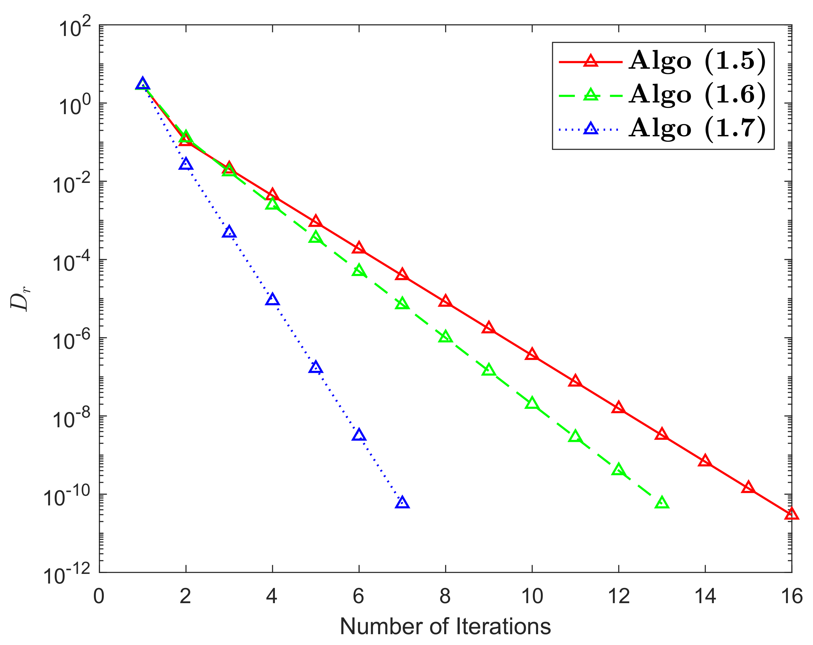
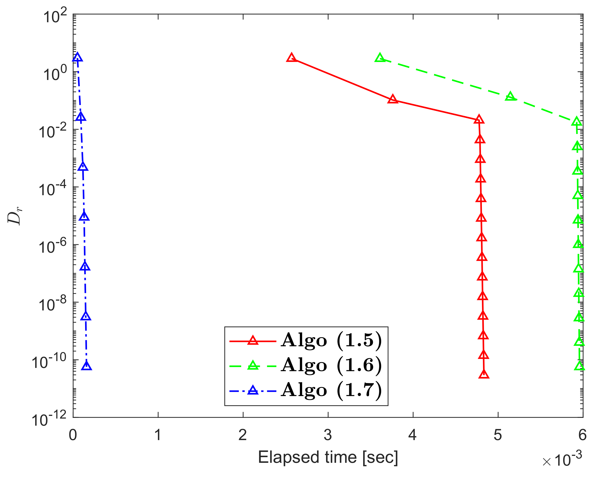
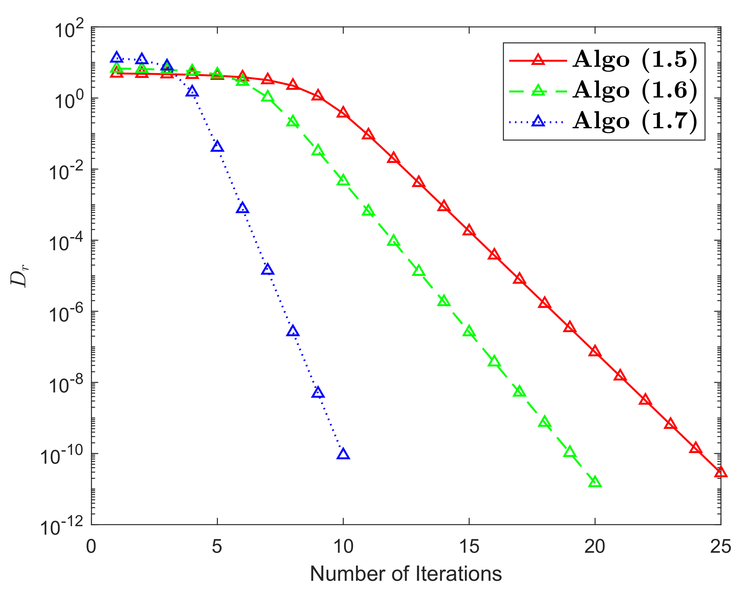
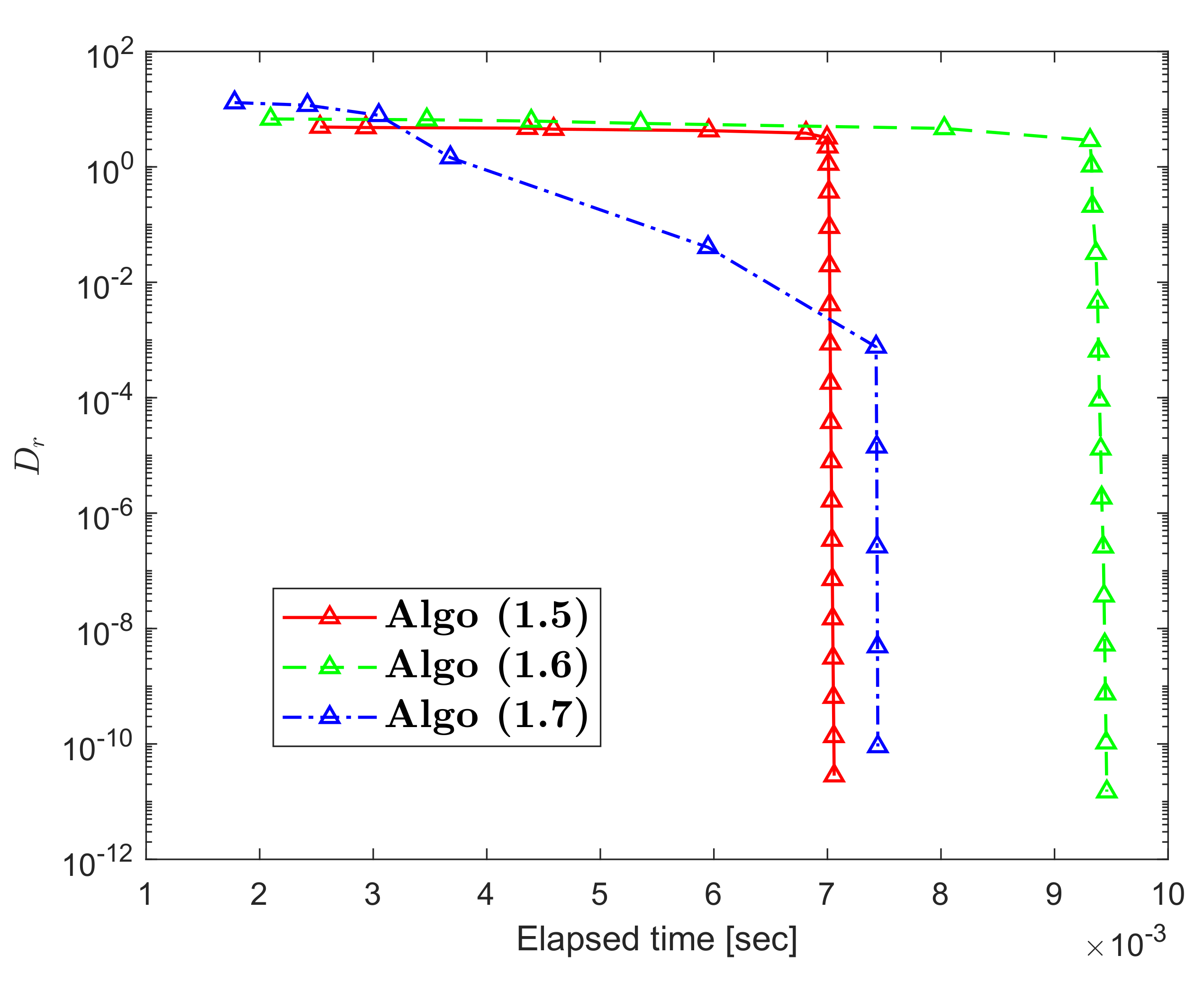
6. Numerical Example

In this part, we provide an illustrative example of an RSTN mapping that does not meet condition $\left(C\right)$. We also assess the convergence of the HR${}^{*}$ iterative scheme in comparison to some of the most popular iterative schemes in the literature.

 Example 4. 

Consider $\left(\mathbb{R},∥.∥\right)$ as a BS equipped with the usual norm and $\mathrm{\Delta }=[3,5].$ Define a mapping $\Im :\mathrm{\Delta }\to \mathrm{\Delta }$ by

$$\Im \varpi =\left\{\begin{array}{cc}\frac{\varpi +6}{3},& if\varpi <5,\\ 2,& if\varpi =5.\end{array}\right.$$

In order to prove that ℑ does not satisfy condition (C), we take $\varpi =4$ and $\upsilon =5,$ hence

$$\frac{1}{2}\left|\varpi -\Im \varpi \right|=\frac{1}{2}\left|4-\Im 4\right|=\frac{1}{3}<1=\left|\varpi -\upsilon \right|.$$

However,

$$\left|\Im \varpi -\Im \upsilon \right|\le \left|\Im 4-\Im 5\right|=\left|\frac{10}{3}-\frac{6}{3}\right|=\frac{4}{3}>1=\left|\varpi -\upsilon \right|.$$

Now, to show that ℑ is an RSTN mapping, we consider the cases below:

 (I) 

If $\varpi ,\upsilon <5,$ we get

$$\begin{array}{ccc}& & \ell \left|\varpi -\Im \varpi \right|+\ell \left|\upsilon -\Im \upsilon \right|+(1-2\ell )\left|\varpi -\upsilon \right|\hfill \\ & =& \frac{1}{2}\left|\varpi -\left(\frac{\varpi +6}{3}\right)\right|+\frac{1}{2}\left|\upsilon -\left(\frac{\upsilon +6}{3}\right)\right|\hfill \\ & =& \frac{1}{2}\left|\frac{2\varpi -6}{3}\right|+\frac{1}{2}\left|\frac{2\upsilon -6}{3}\right|\hfill \\ & \ge & \frac{1}{2}\left|\left(\frac{2\varpi -6}{3}\right)-\left(\frac{2\upsilon -6}{3}\right)\right|\hfill \\ & =& \frac{1}{2}\left|\frac{2\varpi }{3}-\frac{2\upsilon }{3}\right|=\frac{1}{3}\left|\varpi -\upsilon \right|=\left|\Im \varpi -\Im \upsilon \right|.\hfill \end{array}$$

 (II) 

If $\varpi <5$ and $\upsilon =5,$ we obtain

$$\begin{array}{ccc}& & \ell \left|\varpi -\Im \varpi \right|+\ell \left|\upsilon -\Im \upsilon \right|+(1-2\ell )\left|\varpi -\upsilon \right|\hfill \\ & =& \frac{1}{2}\left|\varpi -\left(\frac{\varpi +6}{3}\right)\right|+\frac{1}{2}\left|5-2\right|\hfill \\ & =& \frac{1}{2}\left|\frac{2\varpi -6}{3}\right|+\frac{3}{2}=\left|\frac{\varpi }{3}\right|+\frac{1}{2}\hfill \\ & \ge & \left|\frac{\varpi }{3}\right|=\left|\Im \varpi -\Im \upsilon \right|.\hfill \end{array}$$

 (III) 

If $\upsilon <5$ and $\varpi =5,$ we have

$$\begin{array}{ccc}& & \ell \left|\varpi -\Im \varpi \right|+\ell \left|\upsilon -\Im \upsilon \right|+(1-2\ell )\left|\varpi -\upsilon \right|\hfill \\ & =& \frac{1}{2}\left|5-2\right|+\frac{1}{2}\left|\upsilon -\left(\frac{\upsilon +6}{3}\right)\right|\hfill \\ & =& \frac{3}{2}+\frac{1}{2}\left|\frac{2\upsilon -6}{3}\right|=\frac{1}{2}+\left|\frac{\upsilon }{3}\right|\hfill \\ & \ge & \left|\frac{\upsilon }{3}\right|=\left|\Im \varpi -\Im \upsilon \right|.\hfill \end{array}$$

• If $\upsilon =\varpi =5,$ we can write

  $$\begin{array}{ccc}& & \ell \left|\varpi -\Im \varpi \right|+\ell \left|\upsilon -\Im \upsilon \right|+(1-2\ell )\left|\varpi -\upsilon \right|\hfill \\ & =& 3>0=\left|2-\Im \upsilon \right|=\left|\Im \varpi -\Im \upsilon \right|.\hfill \end{array}$$

Hence, ℑ is RSTN mapping and has a unique FP $3.$

Numerically, by using MATLAB R2015a, we found that our iterative scheme converges faster than both iterations (5) and (6) according to

Table 1. Numerical comparison of results of Algorithms (5)–(7).

	Number of Iterations
Initial Point (${\mathit{z}}_{\mathbf{1}}$)	Algorithm (5)	Algorithms (6)	Algorithms (7)
$3.00$	16	13	7
$3.82$	23	18	10
$4.44$	25	20	10

and

Table 2. Numerical comparison of results of Algorithms (5)–(7).

	Execution Time in Seconds
Initial Point (${\mathit{z}}_{\mathbf{1}}$)	Algorithm (5)	Algorithms (6)	Algorithms (6)
$3.00$	0.00483290000000000	0.00595750000000000	0.000157200000000000
$3.82$	0.00236760000000000	0.00755520000000000	0.00779860000000000
$4.44$	0.00705930000000000	0.00946030000000000	0.00744400000000000

and Figure 1, Figure 2, Figure 3, Figure 4, Figure 5 and Figure 6 as follows:

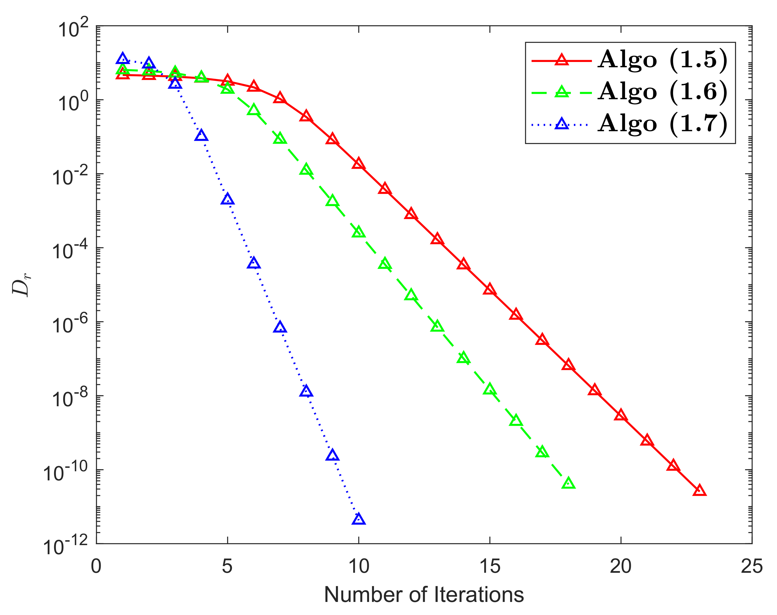
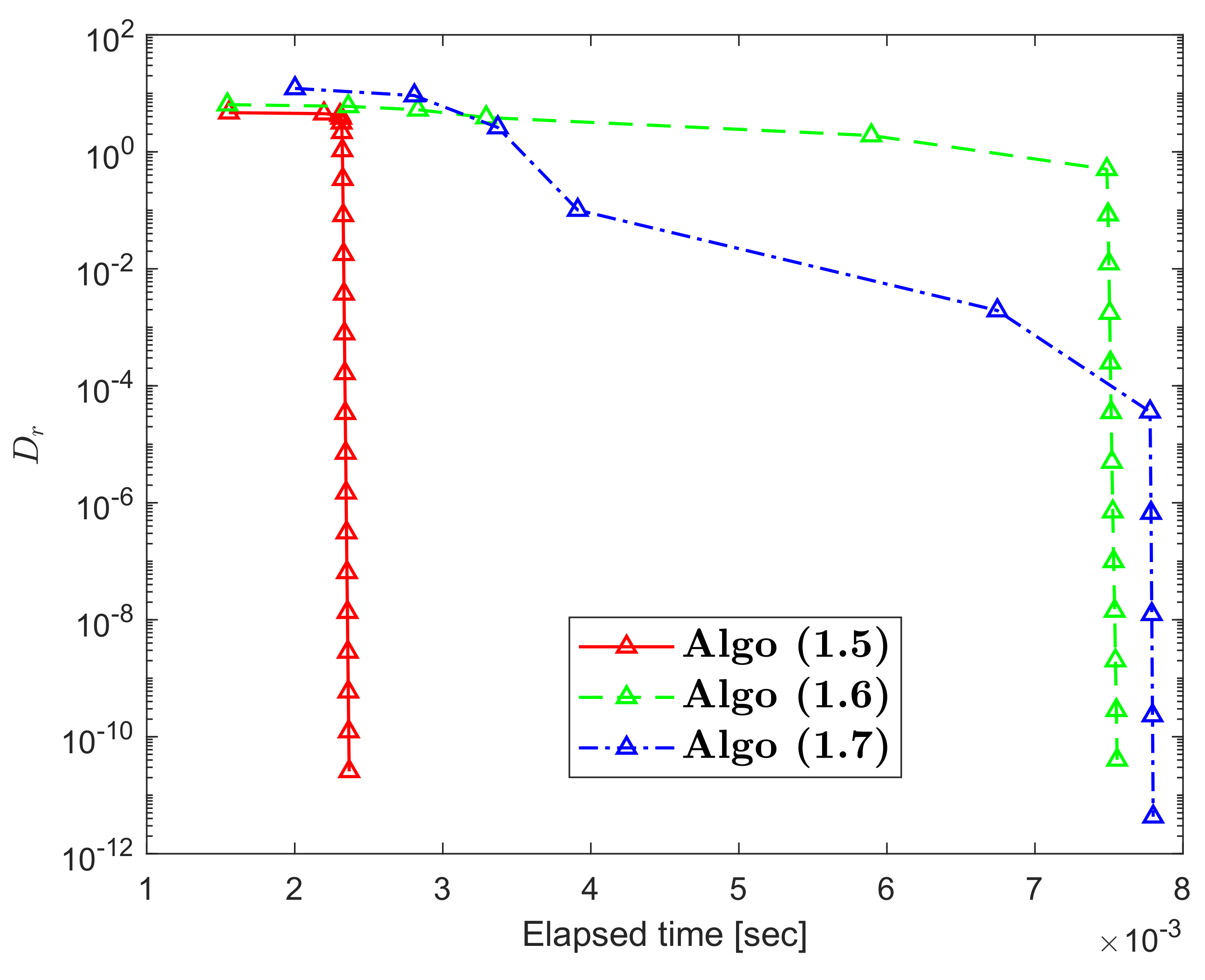
7. Solving 2D Volterra Integral Equation

In this section, we investigate how our main results can be applied to the nonlinear 2D Volterra integral equation of the form:

$$\begin{array}{ccc}\hfill \varkappa (\lambda ,\delta )& =& \beta (\lambda ,\delta )+\underset{0}{\overset{\lambda }{\int }}\underset{0}{\overset{\delta }{\int }}{\mathrm{\Omega }}_1\left(r,u,\varkappa (r,u)\right)drdu\hfill \\ & & +\eta \underset{0}{\overset{\lambda }{\int }}{\mathrm{\Omega }}_2\left(\delta ,u,\varkappa (\lambda ,u)\right)du+\gamma \underset{0}{\overset{\delta }{\int }}{\mathrm{\Omega }}_3\left(\lambda ,r,\varkappa (\delta ,r)\right)dr,\hfill \end{array}$$

(34)

for all $\lambda ,\delta ,r,u\in [0,1],$ where $\varkappa \in \mathrm{\Lambda }\times \mathrm{\Lambda },$$\beta :[0,1]\times [0,1]\to {\mathbb{R}}^2,$${\mathrm{\Omega }}_i(i=1,2,3):[0,1]\times [0,1]\times {\mathbb{R}}^2\to {\mathbb{R}}^2,$$\eta ,\gamma \ge 0$ and $\mathrm{\Lambda }=C\left([0,1]\right)$ is a BS with the maximum norm

$${∥\varpi -\upsilon ∥}_{\infty }=\underset{\tau \in [0,1]}{max}\left|\varpi \left(\tau \right)-\upsilon \left(\tau \right)\right|,\mathrm{for}\mathrm{all}\varpi ,\upsilon \in C\left([0,1]\right).$$

Now, our main theorem here is as follows:

 Theorem 8. 

Assume that ℧ is a nonempty closed convex subset of Λ and $\Im :\mho \to \mho$ described as

$$\begin{array}{ccc}\hfill \Im \varkappa (\lambda ,\delta )& =& \beta (\lambda ,\delta )+\underset{0}{\overset{\lambda }{\int }}\underset{0}{\overset{\delta }{\int }}{\mathrm{\Omega }}_1\left(r,u,\varkappa (r,u)\right)drdu\hfill \\ & & +\eta \underset{0}{\overset{\lambda }{\int }}{\mathrm{\Omega }}_2\left(\delta ,u,\varkappa (\lambda ,u)\right)du+\gamma \underset{0}{\overset{\delta }{\int }}{\mathrm{\Omega }}_3\left(\lambda ,r,\varkappa (\delta ,r)\right)dr.\hfill \end{array}$$

Assume also the assertions below are true

$\left(A_1\right)$

the function $\varkappa :\mathrm{\Lambda }\times \mathrm{\Lambda }\to {\mathbb{R}}^2$ is continuous;

$\left(A_2\right)$

the functions ${\mathrm{\Omega }}_i(i=1,2,3):[0,1]\times [0,1]\times {\mathbb{R}}^2\to {\mathbb{R}}^2$ are continuous and there are the constants ${\ell }_1,{\ell }_2,{\ell }_3>0$ so that

$$\begin{array}{ccc}\hfill \left|{\mathrm{\Omega }}_1\left(r,u,{\varpi }_1(r,u)\right)-{\mathrm{\Omega }}_1\left(r,u,{\varpi }_2(r,u)\right)\right|& \le & {\ell }_1\left|{\varpi }_1-{\varpi }_2\right|,\hfill \\ \hfill \left|{\mathrm{\Omega }}_2\left(r,u,{\varpi }_1(r,u)\right)-{\mathrm{\Omega }}_2\left(r,u,{\varpi }_2(r,u)\right)\right|& \le & {\ell }_2\left|{\varpi }_1-{\varpi }_2\right|,\hfill \\ \hfill \left|{\mathrm{\Omega }}_3\left(r,u,{\varpi }_1(r,u)\right)-{\mathrm{\Omega }}_3\left(r,u,{\varpi }_2(r,u)\right)\right|& \le & {\ell }_3\left|{\varpi }_1-{\varpi }_2\right|,\hfill \end{array}$$

for ${\varpi }_1,{\varpi }_2\in {\mathbb{R}}^2;$

$\left(A_3\right)$

for $\eta ,\gamma \ge 0,$${\ell }_1+\eta {\ell }_2+\gamma {\ell }_3\le \xi ,$ where $\xi \in (0,1).$

Then, the 2D Volterra integral Equation (34) has a solution in $\mho \times \mho$ provided that ℑ has an FP.

 Proof. 

Let $\varkappa ,{\varkappa }^{*}\in \mathrm{\Lambda }\times \mathrm{\Lambda },$ then

$$\begin{array}{ccc}\hfill {∥\varkappa -\Im {\varkappa }^{*}∥}_{\infty }& =& \underset{\tau \in [0,1]}{max}\left|\varkappa (\lambda ,\delta )\left(\tau \right)-\Im {\varkappa }^{*}(\lambda ,\delta )\right|\hfill \\ & =& \underset{\tau \in [0,1]}{max}\left|\varkappa (\lambda ,\delta )\left(\tau \right)-\beta (\lambda ,\delta )\left(\tau \right)-\underset{0}{\overset{\lambda }{\int }}\underset{0}{\overset{\delta }{\int }}{\mathrm{\Omega }}_1\left(r,u,{\varkappa }^{*}(r,u)\right)drdu\right.\hfill \\ & & \left.-\eta \underset{0}{\overset{\lambda }{\int }}{\mathrm{\Omega }}_2\left(\delta ,u,{\varkappa }^{*}(\lambda ,u)\right)du-\gamma \underset{0}{\overset{\delta }{\int }}{\mathrm{\Omega }}_3\left(\lambda ,r,{\varkappa }^{*}(\delta ,r)\right)dr\right|\hfill \\ & \le & \underset{\tau \in [0,1]}{max}\left\{\left|\varkappa (\lambda ,\delta )\left(\tau \right)-\beta (\lambda ,\delta )\left(\tau \right)-\underset{0}{\overset{\lambda }{\int }}\underset{0}{\overset{\delta }{\int }}{\mathrm{\Omega }}_1\left(r,u,\varkappa (r,u)\right)drdu\right.\right.\hfill \\ & & \left.-\eta \underset{0}{\overset{\lambda }{\int }}{\mathrm{\Omega }}_2\left(\delta ,u,\varkappa (\lambda ,u)\right)du-\gamma \underset{0}{\overset{\delta }{\int }}{\mathrm{\Omega }}_3\left(\lambda ,r,\varkappa (\delta ,r)\right)dr\right|\hfill \\ & & +\left|\underset{0}{\overset{\lambda }{\int }}\underset{0}{\overset{\delta }{\int }}{\mathrm{\Omega }}_1\left(r,u,\varkappa (r,u)\right)drdu-\underset{0}{\overset{\lambda }{\int }}\underset{0}{\overset{\delta }{\int }}{\mathrm{\Omega }}_1\left(r,u,{\varkappa }^{*}(r,u)\right)drdu\right|\hfill \\ & & +\eta \left|\underset{0}{\overset{\lambda }{\int }}{\mathrm{\Omega }}_2\left(\delta ,u,\varkappa (\lambda ,u)\right)du-\underset{0}{\overset{\lambda }{\int }}{\mathrm{\Omega }}_2\left(\delta ,u,{\varkappa }^{*}(\lambda ,u)\right)du\right|\hfill \\ & & \left.+\gamma \left|\underset{0}{\overset{\delta }{\int }}{\mathrm{\Omega }}_3\left(\lambda ,r,\varkappa (\delta ,r)\right)dr-\gamma \underset{0}{\overset{\delta }{\int }}{\mathrm{\Omega }}_3\left(\lambda ,r,{\varkappa }^{*}(\delta ,r)\right)dr\right|\right\}\hfill \\ & \le & \underset{\tau \in [0,1]}{max}\left|\varkappa (\lambda ,\delta )\left(\tau \right)-\Im \varkappa (\lambda ,\delta )\right|\hfill \\ & & +{\ell }_1\underset{\tau \in [0,1]}{max}\underset{0}{\overset{\lambda }{\int }}\underset{0}{\overset{\delta }{\int }}\left|\varkappa (r,u)-{\varkappa }^{*}(r,u)\right|drdu+\eta {\ell }_2\underset{\tau \in [0,1]}{max}\underset{0}{\overset{\lambda }{\int }}\left|\varkappa (r,u)-{\varkappa }^{*}(r,u)\right|du\hfill \\ & & +\gamma {\ell }_3\underset{\tau \in [0,1]}{max}\underset{0}{\overset{\delta }{\int }}\left|\varkappa (r,u)-{\varkappa }^{*}(r,u)\right|dr,\hfill \end{array}$$

which implies that

$$\begin{array}{ccc}\hfill {∥\varkappa -\Im {\varkappa }^{*}∥}_{\infty }& \le & \underset{\tau \in [0,1]}{max}\left|\varkappa (\lambda ,\delta )\left(\tau \right)-\Im \varkappa (\lambda ,\delta )\right|\hfill \\ & & +\underset{\tau \in [0,1]}{max}{\ell }_1\left|\varkappa (r,u)-{\varkappa }^{*}(r,u)\right|+\eta {\ell }_2\underset{\tau \in [0,1]}{max}\left|\varkappa (r,u)-{\varkappa }^{*}(r,u)\right|\hfill \\ & & +\gamma {\ell }_3\underset{\tau \in [0,1]}{max}\left|\varkappa (r,u)-{\varkappa }^{*}(r,u)\right|\hfill \\ & \le & {∥\varkappa -\Im {\varkappa }^{*}∥}_{\infty }+({\ell }_1+\eta {\ell }_2+\gamma {\ell }_3)\underset{\tau \in [0,1]}{max}\left|\varkappa (r,u)-{\varkappa }^{*}(r,u)\right|\hfill \\ & \le & {∥\varkappa -\Im {\varkappa }^{*}∥}_{\infty }+\xi {∥\varkappa -{\varkappa }^{*}∥}_{\infty }\hfill \\ & \le & {∥\varkappa -\Im {\varkappa }^{*}∥}_{\infty }+{∥\varkappa -{\varkappa }^{*}∥}_{\infty }.\hfill \end{array}$$

Hence, by Lemma 4, ℑ is an RSTN mapping because it fulfills the condition (10) on ℧ with $\left(\frac{3+\ell }{1-\ell }\right)=1.$ Set $\mho =\mathrm{\Delta }$ and $\mathrm{\Lambda }=\mathrm{\Pi },$ we find that all requirements of Lemma 6 are satisfied. Therefore, ℑ has at least one FP. Thus, problem (33) has a solution on $\mho \times \mho .$ □

The following example support Theorem 8:

 Example 5. 

Consider the following 2D Volterra integral equation

$$\varkappa (\lambda ,\delta )=\frac{\pi }{2}\lambda -\frac{{\delta }^2}{7\pi }+\underset{0}{\overset{\lambda }{\int }}\underset{0}{\overset{\delta }{\int }}\frac{cos\varkappa \left(ru\right)}{2}drdu+\frac{2}{7}\underset{0}{\overset{\lambda }{\int }}\frac{cos\varkappa \left(\lambda u\right)}{2}du+\frac{1}{7}\underset{0}{\overset{\delta }{\int }}\frac{cos\varkappa \left(\delta r\right)}{2}dr.$$

(35)

It is clear that problem (35) is a special case of (34) with

$$\begin{array}{ccc}\hfill \beta (\lambda ,\delta )& =& \frac{\pi }{2}\lambda -\frac{{\delta }^2}{7\pi },{\mathrm{\Omega }}_1\left(r,u,\varkappa (r,u)\right)=\frac{cos\varkappa \left(ru\right)}{2},\hfill \\ \hfill {\mathrm{\Omega }}_2\left(\delta ,u,\varkappa (\lambda ,u)\right)& =& \frac{cos\varkappa \left(\lambda u\right)}{2},{\mathrm{\Omega }}_3\left(\lambda ,r,\varkappa (\delta ,r)\right)=\frac{cos\varkappa \left(\delta r\right)}{2},\eta =\frac{2}{7}\mathrm{and}\gamma =\frac{1}{7}.\hfill \end{array}$$

Then, for any $r,u\in [0,1]$ and ${\varpi }_1,{\varpi }_2\in {\mathbb{R}}^2,$ we find that

$$\begin{array}{ccc}\hfill \left|{\mathrm{\Omega }}_1\left(r,u,{\varpi }_1(r,u)\right)-{\mathrm{\Omega }}_1\left(r,u,{\varpi }_2(r,u)\right)\right|& \le & \frac{1}{2}\left|cos{\varpi }_1-cos{\varpi }_2\right|,\hfill \\ \hfill \left|{\mathrm{\Omega }}_2\left(r,u,{\varpi }_1(r,u)\right)-{\mathrm{\Omega }}_2\left(r,u,{\varpi }_2(r,u)\right)\right|& \le & \frac{1}{2}\left|cos{\varpi }_1-cos{\varpi }_2\right|,\hfill \\ \hfill \left|{\mathrm{\Omega }}_3\left(r,u,{\varpi }_1(r,u)\right)-{\mathrm{\Omega }}_3\left(r,u,{\varpi }_2(r,u)\right)\right|& \le & \frac{1}{2}\left|cos{\varpi }_1-cos{\varpi }_2\right|,\hfill \end{array}$$

(36)

According to the mean-value theorem, for any ${\varpi }_1,{\varpi }_2\in {\mathbb{R}}^2$ with ${\varpi }_1<{\varpi }_2$ there is $b\in \left[{\varpi }_1,{\varpi }_2\right]$ so that

$$\frac{cos{\varpi }_1-cos{\varpi }_2}{{\varpi }_1-{\varpi }_2}=-sin\left(b\right),\mathrm{implies}\frac{\left|cos{\varpi }_1-cos{\varpi }_2\right|}{\left|{\varpi }_1-{\varpi }_2\right|}=\left|-sin\left(b\right)\right|\le 1.$$

Hence, $\left|cos{\varpi }_1-cos{\varpi }_2\right|\le \left|{\varpi }_1-{\varpi }_2\right|$ and (36) reduces to

$$\begin{array}{ccc}\hfill \left|{\mathrm{\Omega }}_1\left(r,u,{\varpi }_1(r,u)\right)-{\mathrm{\Omega }}_1\left(r,u,{\varpi }_2(r,u)\right)\right|& \le & \frac{1}{2}\left|{\varpi }_1-{\varpi }_2\right|,\hfill \\ \hfill \left|{\mathrm{\Omega }}_2\left(r,u,{\varpi }_1(r,u)\right)-{\mathrm{\Omega }}_2\left(r,u,{\varpi }_2(r,u)\right)\right|& \le & \frac{1}{2}\left|{\varpi }_1-{\varpi }_2\right|,\hfill \\ \hfill \left|{\mathrm{\Omega }}_3\left(r,u,{\varpi }_1(r,u)\right)-{\mathrm{\Omega }}_3\left(r,u,{\varpi }_2(r,u)\right)\right|& \le & \frac{1}{2}\left|{\varpi }_1-{\varpi }_2\right|,\hfill \end{array}$$

where ${\ell }_1={\ell }_2={\ell }_3=\frac{1}{2}$ and ${\ell }_1+\eta {\ell }_2+\gamma {\ell }_3=\xi =\frac{5}{7}<1.$ It is easy to see that $\beta (\lambda ,\delta )$ is continuous on $[0,1]$.

Consequently, all conditions of Theorem 8 are satisfied. Therefore, there exists a solution to the problem (36).

8. Conclusions and Future Works

In this study, a four-step iterative scheme known as the $H{R}^{*}$—iterative scheme (7) is presented for approximating the fixed points of contractive-like mappings and RSTN mappings. Analytically, it has been demonstrated that the new iterative scheme converges faster than the iterative method (5) for contractive-like mappings. Furthermore, we have shown numerically that for contractive-like mappings, our novel iterative method converges faster than several popular iterative schemes in the literature. Additionally, the ${\omega }^2$—stability result of the $H{R}^{*}$—iterative scheme (7) has also been obtained. To clarify the idea of ${\omega }^2$—stability of the considered algorithm with regard to ℑ, we have given an example. Additionally, we have demonstrated a number of weak and strong convergence theorems for RSTN mappings in uniformly convex BSs. In order to compare the convergence behavior of the proposed algorithm (7) with certain well-known iterative schemes, a novel example of RSTN mappings has been supplied. As a practical application, we proved that a 2D Volterra integral equation has a solution. Additionally, we provided an engaging example to explain the outcome of our application. Finally, as future work for this paper, we suggest the following:

(1)

If we define a mapping ℑ in a Hilbert space $\mathrm{\Delta }$ endowed with inner product space, we can find a common solution to the variational inequality problem by using our iteration (7). This problem can be stated as follows: find ${\wp }^{*}\in \mathrm{\Delta }$ such that

$$\langle \Im {\wp }^{*},\wp -{\wp }^{*}\rangle \ge 0\mathrm{for}\mathrm{all}\wp \in \mathrm{\Delta },$$

where $\Im :\mathrm{\Delta }\to \mathrm{\Delta }$ is a nonlinear mapping. Variational inequalities are an important and essential modeling tool in many fields such as engineering mechanics, transportation, economics, and mathematical programming, see [45,46,47].

(2)

We can generalize our algorithm to gradient and extra-gradient projection methods, these methods are very important for finding saddle points and solving many problems in optimization, see [6].

(3)

We can accelerate the convergence of the proposed algorithm by adding shrinking projection and CQ terms. These methods stimulate algorithms and improve their performance to obtain strong convergence, for more details, see [7].

(4)

If we consider the mapping ℑ as an $\alpha$—inverse strongly monotone and the inertial term is added to our algorithm, then we have the inertial proximal point algorithm. This algorithm is used in many applications such as monotone variational inequalities, image restoration problems, convex optimization problems, and split convex feasibility problems, see [48,49,50]. For more accuracy, these problems can be expressed as mathematical models such as machine learning and the linear inverse problem.

(5)

We can try to determine the error of our present iteration.

References

1. Arias, A.; Gheondea, A.; Gudder, S. Fixed points of quantum operations. J. Math. Phys. 2002, 43, 5872. [Google Scholar] [CrossRef] [Green Version]
2. Lan, K.Q.; Wu, J.H. A fixed-point theorem and applications to problems on sets with convex sections and to Nash equilibria. Math. Comput. Mod. 2002, 36, 139–145. [Google Scholar] [CrossRef]
3. Amar, A.B.; Jeribi, A.; Mnif, M. Some fixed point theorems and application to bio-logical model. Numer. Funct. Anal. Optim. 2008, 29, 1–23. [Google Scholar] [CrossRef]
4. Eke, K.S.; Olisama, V.O.; Bishop, S.A.; Liu, L. Some fixed point theorems for convex contractive mappings in complete metric spaces with applications. Cogent Math. Stat. 2019, 6, 1655870. [Google Scholar] [CrossRef]
5. Georgescu, F. IFS consisting of generalized convex contractions. Anal. Stiintifice Ale Univers. Ovidius Const. 2017, 25, 77–86. [Google Scholar]
6. Korpelevich, G.M. The extragradient method for finding saddle points and other problems. Ekon. Mat. Metod. 1976, 12, 747–756. [Google Scholar]
7. Martinez-Yanes, C.; Xu, H.K. Strong convergence of the CQ method for fixed point iteration processes. Nonlinear Anal. 2006, 64, 2400–2411. [Google Scholar] [CrossRef]
8. Bauschke, H.H.; Combettes, P.L. Convex Analysis and Monotone Operator Theory in Hilbert Spaces; Springer: Berlin, Germany, 2011. [Google Scholar]
9. Adamu, A.; Kitkuan, D.; Padcharoen, A.; Chidume, C.E.; Kumam, P. Inertial viscosity-type iterative method for solving inclusion problems with applications. Math. Comput. Simul. 2022, 194, 445–459. [Google Scholar] [CrossRef]
10. Adamu, A.; Deepho, J.; Ibrahim, A.H.; Abubakar, A.B. Approximation of zeros of sum of monotone mappings with applications to variational inequality and image restoration problems. Nonlinear Funct. Anal. Appl. 2021, 26, 411–432. [Google Scholar]
11. Tuyen, T.M.; Hammad, H.A. Effect of shrinking projection and CQ-methods on two inertial forward–backward algorithms for solving variational inclusion problems. Rend. Circ. Mat. Palermo II Ser. 2021, 70, 1669–1683. [Google Scholar] [CrossRef]
12. Watcharaporna, C.; Damrongsak, Y.; Hammad, H.A. Modified hybrid projection methods with SP iterations for quasi-nonexpansive multivalued mappings in Hilbert spaces. Bull. Iran. Math. Soc. 2021, 47, 1399–1422. [Google Scholar]
13. Picard, E. Memoire sur la theorie des equations aux derivees partielles et la methode des approximations successives. J. Math. Pures et Appl. 1890, 6, 145–210. [Google Scholar]
14. Halpern, B. Fixed points of nonexpanding maps. Bull. Am. Math. Soc. 1967, 73, 957–961. [Google Scholar] [CrossRef] [Green Version]
15. He, S.; Yang, C. Boundary point algorithms for minimum norm fixed points of nonexpansive mappings. Fixed Point Theory Appl. 2014, 2014, 56. [Google Scholar] [CrossRef] [Green Version]
16. Hammad, H.A.; Rahman, H.u.; De la Sen, M. Shrinking projection methods for accelerating relaxed inertial Tseng-type algorithm with applications. Math. Probl. Eng. 2020, 2020, 7487383. [Google Scholar] [CrossRef]
17. Hammad, H.A.; Rahman, H.u.; De la Sen, M. Advanced algorithms and common solutions to variational inequalities. Symmetry 2020, 12, 1198. [Google Scholar] [CrossRef]
18. Zamfirescu, T. Fixed point theorems in metric spaces. Arch. Math. 1972, 23, 292–298. [Google Scholar] [CrossRef]
19. Berinde, V. On the approximation of fixed points of weak contractive mappings. Carpath. J. Math. 2003, 19, 7–22. [Google Scholar]
20. Suzuki, T. Fixed point theorems and convergence theorems for some generalized nonexpansive mappings. J. Math. Anal. Appl. 2008, 340, 1088–1095. [Google Scholar] [CrossRef] [Green Version]
21. Pant, R.; Pandey, R. Existence and convergence results for a class of non-expansive type mappings in hyperbolic spaces. Appl. Gen. Topol. 2019, 20, 281–295. [Google Scholar] [CrossRef]
22. Mann, W.R. Mean value methods in iteration. Proc. Am. Math. Soc. 1953, 4, 506–510. [Google Scholar] [CrossRef]
23. Ishikawa, S. Fixed points by a new iteration method. Proc. Am. Math. Soc. 1974, 44, 147–150. [Google Scholar] [CrossRef]
24. Noor, M.A. New approximation schemes for general variational inequalities. J. Math. Anal. Appl. 2000, 251, 217–229. [Google Scholar] [CrossRef] [Green Version]
25. Agarwal, R.P.; Regan, D.O.; Sahu, D.R. Iterative construction of fixed points of nearly asymptotically nonexpansive mappings. J Nonlinear Convex Anal. 2007, 8, 61–79. [Google Scholar]
26. Abbas, M.; Nazir, T. A new faster iteration process applied to constrained minimization and feasibility problems. Math. Vesn. 2014, 66, 223–234. [Google Scholar]
27. Chugh, R.; Kumar, V.; Kumar, S. Strong convergence of a new three step iterative scheme in Banach spaces. Am. J. Comp. Math. 2012, 2, 345–357. [Google Scholar] [CrossRef] [Green Version]
28. Sahu, D.R.; Petrusel, A. Strong convergence of iterative methods by strictly pseudocontractive mappings in Banach spaces. Nonlinear Anal. Theory Methods Appl. 2011, 74, 6012–6023. [Google Scholar] [CrossRef]
29. Gursoy, F.; Karakaya, V. A Picard-S hybrid type iteration method for solving a differential equation with retarded argument. arXiv 2014, arXiv:1403.2546v2. [Google Scholar]
30. Thakur, B.S.; Thakur, D.; Postolache, M. A new iterative scheme for numerical reckoning fixed points of Suzuki’s generalized nonexpansive mappings. Appl. Math. Comput. 2016, 275, 147–155. [Google Scholar] [CrossRef]
31. Ullah, K.; Arshad, M. Numerical reckoning fixed points for Suzuki’s generalized nonexpansive mappings via new iteration process. Filomat 2018, 32, 187–196. [Google Scholar] [CrossRef] [Green Version]
32. Ahmad, J.; Ullah, K.; Arshad, M.; Ma, Z. A new iterative method for Suzuki mappings in Banach spaces. J. Math. 2021, 2021, 6622931. [Google Scholar] [CrossRef]
33. Hammad, H.A.; Rehman, H.u.; Zayed, M. Applying faster algorithm for obtaining convergence, stability, and data dependence results with application to functional-integral equations. AIMS Math. 2022, 7, 19026–19056. [Google Scholar] [CrossRef]
34. Berinde, V. Picard iteration converges faster than Mann iteration for a class of quasicontractive operators. Fixed Point Theory Appl. 2004, 2, 97–105. [Google Scholar] [CrossRef] [Green Version]
35. Senter, H.F.; Dotson, W.G. Approximating fixed points of nonexpansive mapping. Proc. Am. Math. Soc. 1974, 44, 375–380. [Google Scholar] [CrossRef]
36. Weng, X. Fixed point iteration for local strictly pseudocontractive mapping. Proc. Am. Math. Soc. 1991, 113, 727–731. [Google Scholar] [CrossRef]
37. Ullah, K.; Ahmad, J.; De la Sen, M. On generalized nonexpansive maps in Banach spaces. Computer 2020, 8, 61. [Google Scholar] [CrossRef]
38. Harder, A.M. Fixed Point Theory and Stability Results for Fixed-Point Iteration Procedures. Ph.D. Thesis, University of Missouri-Rolla, St. Rolla, MO, USA, 1987. [Google Scholar]
39. Hammad, H.A.; Rahman, H.u.; De la Sen, M. A novel four-step iterative scheme for approximating the fixed point with a supportive application. Inf. Sci. Lett. 2021, 10, 333–339. [Google Scholar]
40. Okeke, G.A.; Abbas, M.; Sen, M.D. Approximation of the fixed point of multivalued quasi-nonexpansive mappings via a faster iterative process with applications. Discrete Dyn. Nat. Soc. 2020, 2020, 8634050. [Google Scholar] [CrossRef]
41. Berinde, V. Iterative Approximation of Fixed Points; Springer: Berlin, Germany, 2007. [Google Scholar]
42. Timis, I. On the weak stability of Picard iteration for some contractive type mappings and coincidence theorems. Int. J. Comput. Appl. 2012, 37, 9–13. [Google Scholar] [CrossRef]
43. Cardinali, T.; Rubbioni, P. A generalization of the Caristi fixed point theorem in metric spaces. Fixed Point Theory 2010, 11, 3–10. [Google Scholar]
44. Khan, S.H.; Kim, J.K. Common fixed points of two nonexpansive mappings by a modified faster iteration scheme. Bull. Korean Math. Soc. 2010, 47, 973–985. [Google Scholar] [CrossRef]
45. Facchinei, F.; Pang, J.S. Finite-Dimensional Variational Inequalities and Complementarity Problems; Springer Series in Operations Research; Springer: New York, NY, USA, 2003; Volume II. [Google Scholar]
46. Konnov, I.V. Combined Relaxation Methods for Variational Inequalities; Springer: Berlin, Germany, 2001. [Google Scholar]
47. Hammad, H.A.; Cholamjiak, W.; Yambangwai, D.; Dutta, H. A modified shrinking projection methods for numerical reckoning fixed points of G-nonexpansive mappings in Hilbert spaces with graph. Miskolc Math. Notes 2019, 20, 941–956. [Google Scholar] [CrossRef]
48. Chen, P.; Huang, J.; Zhang, X. A primal-dual fixed point algorithm for convex separable minimization with applications to image restoration. Inverse Probl. 2013, 29, 025011. [Google Scholar] [CrossRef]
49. Hammad, H.A.; Rehman, H.u.; Almusawa, H. Tikhonov regularization terms for accelerating inertial Mann-Like algorithm with applications. Symmetry 2021, 13, 554. [Google Scholar] [CrossRef]
50. Dang, Y.; Sun, J.; Xu, H. Inertial accelerated algorithms for solving a split feasibility problem. J. Ind. Manag. Optim. 2017, 13, 1383–1394. [Google Scholar] [CrossRef]
Figure 1. A graphical comparison of Algorithms (5)–(7), where z 1 = 3.00 .
Mathematics 10 04257 g001
Figure 2. A graphical comparison of Algorithms (5)–(7), where z 1 = 3.00 .
Mathematics 10 04257 g002
Figure 3. A graphical comparison of Algorithms (5)–(7), where z 1 = 3.82 .
Mathematics 10 04257 g003
Figure 4. A graphical comparison of Algorithms (5)–(7), where z 1 = 3.82 .
Mathematics 10 04257 g004
Figure 5. A graphical comparison of Algorithms (5)–(7), where z 1 = 4.44 .
Mathematics 10 04257 g005
Figure 6. A graphical comparison of Algorithms (5)–(7), where z 1 = 4.44 .
Mathematics 10 04257 g006