Robust Bi-Level Optimization for Maritime Emergency Materials Distribution in Uncertain Decision-Making Environments

Abstract

Maritime emergency materials distribution is a key aspect of maritime emergency responses. To effectively deal with the challenges brought by the uncertainty of the maritime transport environment, the multi-agent joint decision-making location-routing problem of maritime emergency materials distribution (MEMD-LRP) under an uncertain decision-making environment is studied. First, two robust bi-level optimization models of MEMD-LRP are constructed based on the effect of the uncertainty of the ship’s sailing time and demand of emergency materials at the accident point, respectively, on the premise of considering the rescue time window and priority of emergency materials distribution. Secondly, with the help of robust optimization theory and duality theory, the robust optimization models are transformed into robust equivalent models that are easy to solve. Finally, a hybrid algorithm based on the ant colony and tabu search (ACO-TS) algorithm solves multiple sets of numerical cases based on the case design of the Bohai Sea area, and analyzes the influence of uncertain parameters on the decision making of MEMD-LRP. The study of MEMD-LRP under uncertain decision-making environments using bi-level programming and robust optimization methods can help decision makers at different levels of the maritime emergency logistics system formulate emergency material reserve locations and emergency material distribution schemes that can effectively deal with the uncertainty in maritime emergencies.

1. Introduction

As trade activity between countries gradually resumes in the post-epidemic era, maritime transportation, which is responsible for more than 80% of world trade, has rebounded in 2021 with an estimated growth of 3.2% [1]. The increase in maritime transportation activities has also led to a high incidence of maritime accidents, thus posing significant safety risks [2,3,4]. When an accident occurs at sea, a rapid and efficient emergency response becomes a crucial part of the process, and in this process, the distribution of maritime emergency materials plays a key role. In the actual distribution process of maritime emergency materials, due to the suddenness and unpredictability of maritime accidents, and because maritime transportation is affected by complex meteorological and sea conditions and other factors, the emergency materials demand at the accident point and the ship’s sailing time are usually highly uncertain. Research on emergency materials distribution in traditional deterministic decision-making environments is usually difficult to cope with the challenges brought by complex environmental changes, so it is urgent and important to investigate the maritime emergency materials distribution location-routing problem (MEMD-LRP) in uncertain decision-making environments.

Emergency responses to maritime emergencies is a multi-sectoral endeavor that requires different levels of decision-making bodies to participate in decision making. As a joint decision-making problem, MEMD-LRP involves locating shore-based emergency materials reserves and planning routes for emergency materials distribution. The location problem is solved at the strategic decision-making level, and the distribution route planning of emergency materials is determined at the tactical level or operation level. Bi-level programming can be used to solve the problem of joint decision making by different levels of decision makers, which can ensure that a global perspective is taken first, and the interests of the whole situation and each decision-making subject are considered at the same time.

For a long time, society has generally considered emergency rescue to be a matter of the country, thus neglecting the development of commercially operated rescue organizations. In the actual operation of emergency rescues, in addition to government departments, there are also public welfare rescue units and commercial rescue units. The emergence of public welfare rescue units and commercial rescue units not only improves the speed and efficiency of emergency rescues, but also helps to promote social participation. Among them, the interests represented by public welfare rescue units and government departments are consistent, usually taking the fairness of emergency rescue as the main consideration, and taking dissatisfaction, cost, time, and so on, as the goal [5,6]. On the other hand, commercial rescue units will consider the economy of emergency rescue, which is consistent with minimizing the total economic cost of emergency logistics in the literature [7,8]. The commercial rescue system’s systematic network has yet to be expanded, and it should always be the government departments’ responsibility in terms of the macro-unification of command and scheduling.

Therefore, from the perspective of multi-level decision makers that participate in joint decision making, it is necessary to adopt a method of bi-level programming and robust optimization based on the communication and cooperation between emergency management departments and commercial rescue units without considering public welfare rescue units. During the planning period, this paper studies the MEMD-LRP problem considering the rescue time window, the priority of distribution of different kinds of emergency materials, the uncertain emergency materials demand at the accident point, and the uncertain transportation time of emergency materials, and then optimizes the maritime emergency logistics system as a whole to ensure the demand of the accident points can be met, and the total cost of the emergency logistics system can be reduced in different cases. This paper is an extension of Peng et al.’s [9] study on MEMD-LRP in a deterministic decision-making environment. This study can provide optimal location selection and route planning solutions for MEMD-LRP in an uncertain decision-making environment within the planning period. It also offers decision makers a reference basis for addressing various emergency situations.

The following is the rest of the paper. The second part provides an overview of related studies, the third part describes the research problem, the construction, and the transformation of the model in detail, and the fourth part gives the solution analysis. Finally, the fifth part summarizes the paper.

2. Literature Review

The LRP proposal can be traced back to the 1980s [10]. This problem has aroused widespread concern and attracted many scholars to conduct in-depth research. At present, scholars at home and abroad have conducted a lot of research on the various extended models of general logistics LRP and the improvement of the solution methods [11,12,13]. In the innovation of solving methods, to solve the multi-objective chance-constrained programming model under an uncertain transportation time and cost, Lu et al. [14] changed the antennae search of a single beetle to multiple, embedded Dijkstra algorithms, and designed a hybrid beetle swarm optimization algorithm. Lu et al. [15] designed the ant colony system and improved the grey wolf optimization algorithm to solve the fourth party logistics routing problem model through the convergence factor and proportional weight in order to improve the grey wolf optimization algorithm. Şatir Akpunar and Akpinar [16] proposed a hybrid adaptive large neighborhood search algorithm (ALNS) to solve the LRP problem, which improves the performance of the algorithm by combining the variable neighborhood search (VNS) algorithm with the elite local search algorithm. Alamatsaz et al. [17] combines the progressive hedging algorithm (PHA) with a genetic algorithm (GA) to large-scale solve the green capacitated locating-routing problem. As scholars pay attention to the research of emergency logistics, the joint research of emergency logistics and LRP has become one of the hotspots. Earlier emergency logistics LRPs were considered in deterministic environments. Gan and Liu [18] designed a new multi-objective model based on multi-hazard and multi-supplier scenarios, and proposed an improved non-dominated sorting genetic algorithm (NSGA-II) to find the optimal scheduling scheme. Liu et al. [19] studied the location-routing problem in the early stage of an earthquake from a fair perspective, developed the multi-objective model by using a dictionary sequential object optimization method considering emergency window constraints and partial road damage, and designed a hybrid heuristic algorithm to solve the problem.

With the deepening of the research, the emergency logistics LRP problem gradually evolved from a problem in a deterministic decision-making environment to a more relevant problem in an uncertain decision-making environment, and methods such as stochastic programming, fuzzy functions, and robust optimization have gradually become mainstream tools for solving uncertain problems such as demand, time, and so on, in emergency logistics LRP. Ai et al. [20] constructed a discrete nonlinear integer programming model and solved it using a heuristic algorithm after transforming it into a two-stage model in the context of emergency resource distribution in maritime emergency response systems. Zhang et al. [21] studied sustainable multi-warehouse emergency facility LRP with information uncertainty; constructed multi-objective travel time, emergency response cost, and carbon dioxide emission model; designed a hybrid intelligent algorithm integrating an uncertainty simulation- and designed a genetic algorithm to solve it. Afshar and Haghani [22] proposed a comprehensive model for integrated supply chain operations in response to natural disasters that integrates details such as the optimal location of multi-level temporary facilities, vehicle routing, and pickup or delivery schedules in a dynamic environment. Zhang et al. [23] proposed a scenario-based mixed-integer planning model for reliable LRP with the risk of the stochastic disruption of facilities, designing meta-heuristic algorithms based on maximum likelihood sampling methods, route reallocation, a two-stage neighborhood search, and simulated annealing. Ghasemi et al. [24] proposed a mixed-integer mathematical planning model for the location assignment of a multi-objective, multi-commodity, multi-period, multi-vehicle, and modeled-by-scenario-based probabilistic approach for seismic emergency responses, which is solved using improved multi-objective particle swarm optimization, nondominated sequential genetic algorithm, and the epsilon constraint method. Long et al. [25] studied the multi-objective multi-periodic LRP of epidemic logistics considering stochastic demand, proposed a corresponding robust model, and proposed a preference-inspired co-evolutionary algorithm based on Tchebycheff decomposition (PICEA-g-td). Caunhye et al. [26] proposed a two-stage LRP that was transformed into a single-objective solution for the problem of risk management in the case of a disaster with an uncertain demand and infrastructure status. A nonlinear integer open location-routing model was constructed by Wang et al. [27] that considered travel time, total cost, and reliability when distributing post-disaster relief materials, and they proposed a non-dominated sorting differential evolution algorithm and a non-dominated sorting genetic algorithm to solve it. Raeisi et al. [28] constructed a robust fuzzy multi-objective optimization model to solve the hazardous waste management problem, which was solved using various heuristic algorithms and analyzed comparatively. Shen et al. [29] proposed a triangular fuzzy function to obtain the fuzzy demand considering the uncertainty of the demand in the disaster area, constructed a multi-objective model considering the carbon emissions, and used a two-stage hybrid algorithm to solve the problem. Zhang et al. [30] proposed a novel dynamic multi-objective split-delivery location-routing two-stage optimization model for the emergency logistics of offshore oil spill accidents, and developed a hybrid heuristic algorithm to solve it. Ghasemi et al. [31] proposed a scenario-based stochastic multi-objective location-allocation-routing model considering the existence of uncertainty before and after a disaster, which was solved using epsilon constraints and meta-heuristic algorithms.

Some scholars have also considered the problem of joint decision-making by multiple levels of decision makers in solving emergency LRPs in uncertain decision-making environments. Saeidi-Mobarakeh et al. [32] constructed a bi-level programming model with the government as the decision maker at the upper level and the government’s followers as the decision makers at the lower level to solve a hazardous waste management problem under uncertainty, and a robust optimization was used in the multi-part solution methodology. Zhou et al. [33] addressed the uncertainty in the emergency logistics system, investigated the integration of the location of transit facilities and the transportation of relief materials, constructed a gray mixed-integer bi-level nonlinear program, and designed a hybrid genetic algorithm to solve the proposed model. Chen et al. [34] conducted a study on the robustness and sustainability of the port logistics system for emergency materials using a bi-level programming method to achieve coordinated optimization of emergency logistics infrastructure locations and emergency rescue vehicle routing planning, as well as simulation using statistical modeling.

This study comprehensively reviews 10 representative studies in related fields and compares them in several aspects, such as research background, model construction methods, types of emergency materials, time windows, and solution methods, as shown in

Table 1. Comparison with related studies.

Author	Uncertainty	Maritime Emergency	Modeling Method	Emergency Materials	Time Window	Solution Method
Gan and Liu [18]	No	Yes	Multi-objective modeling	Multiple	Yes	Improved NSGA-II
Ai et al. [20]	Yes	Yes	Single-objective modeling	Single	No	Hybrid heuristic algorithm
Zhang et al. [21]	Yes	No	Multi-objective modeling	No	No	Hybrid intelligence algorithm
Zhang et al. [23]	Yes	No	Scenario-based Single-objective modeling	No	No	Metaheuristic approach
Long et al. [25]	Yes	No	Multi-objective multi-stage robust modeling	Yes	No	Preference-inspired coevolutionary algorithm
Wang et al. [27]	Yes	No	Multi-objective modeling	Yes	No	Non-dominated sorting genetic algorithm Non-dominated sorting differential evolution algorithm
Shen et al. [29]	Yes	No	Fuzzy function Multi-objective modeling	No	No	Two-stage hybrid algorithm
Zhang et al. [30]	Yes	Yes	Dynamic multi-objective modeling	No	Yes	Hybrid heuristic algorithm
Zhou et al. [33]	Yes	No	Bi-level programming modeling	Yes	-	Hybrid genetic algorithm
Chen et al. [34]	Yes	Yes (Port)	Bi-level programming modeling	No	No	Statistical methods
This paper	Yes	Yes	Robust bi-level programming modeling	Yes	Yes	Hybrid heuristic algorithm

. Overall, the research for emergency logistics LRPs is richer and deeper, and stochastic programming, fuzzy functions, robust optimization, and bi-level programming decision-making tools are beginning to be applied to emergency logistics LRPs in uncertain decision-making environments. The hybrid heuristic algorithms, which combine the ant colony algorithm, particle swarm algorithm, genetic algorithm, and other algorithms, are widely used in the solution of emergency logistics LRPs. To our limited knowledge, most of the existing studies are based on land-based disasters and emergencies, and even though the literature [20] has investigated the distribution of emergency resources in maritime emergency response systems, only the probability distribution of the demand has been considered. In addition, existing research has focused on the use of multi-objective models, and the bi-level programming method has not been applied to the marine accident LRP of multi-agent joint decision making under uncertain decision environments. Although the literature [34] studied the port logistics system for emergency materials, it did not address the distribution of maritime emergency materials. The purpose of this paper is to make a plan for different levels of decision makers in maritime emergency logistics systems under uncertain decision-making environments. To achieve this, a combination of a bi-level programming method and a robust optimization method is adopted.

3. Mathematical Problem Formulation

3.1. Problem Description

The decision making of MEMD-LRP involves the location of shore-based emergency material reserves and maritime emergency material distribution route planning, which aims to distribute emergency materials with different priorities from the selected emergency material reserves to the accident point based on information such as the location of the potential accident point, and under constraints such as satisfying the time window. But due to the fact that in the actual MEMD-LRP, the ship’s sailing time and the accident point emergency materials demand uncertainty, the location decision and routing planning decision can be significantly affected.

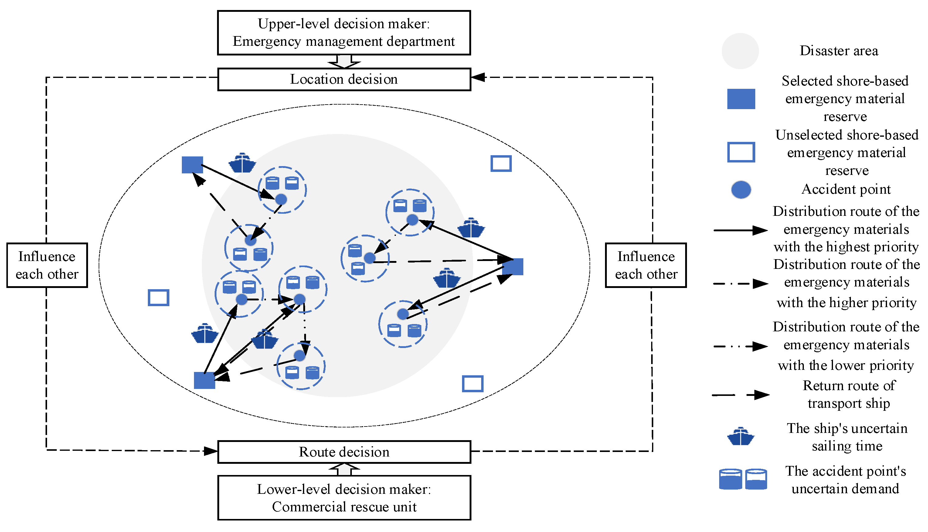
In uncertain decision-making environments, a joint decision-making model with multiple levels of decision makers becomes particularly important. The MEMD-LRP can be described from the perspective of bi-level programming, in which the upper-level decision maker (the emergency management department) integrates the location problem of the emergency reserves. Because the construction of the emergency reserve is required to be outsourced to the manufacturer [35], the emergency management department must consider the emergency reserve stockpile construction cost and accident point time satisfaction loss cost. Lower-level decision makers (commercial rescue units) independently plan emergency material distribution routes based on upper-level decisions to minimize distribution costs, ship transportation costs, ship dispatch costs, and time penalty costs. Rescue units will develop the distribution program feedback to the emergency management department, and according to the response of the rescue units here to make decisions, the interaction between the two is constantly carried out, forming an iterative decision-making process to develop the overall optimal decision to adapt to the maritime emergency’s uncertainty.

The maritime emergency logistics system involving multi-level decision-making agents studied in this paper is shown in Figure 1.

The paper has the following assumptions:

(1)

Commercial rescue units are taken, as the lower-level decision makers of this study and public relief units are not considered;

(2)

Multiple candidates reserve with unrestricted capacity and known locations;

(3)

Multiple potential accident points with known locations, without any consideration of drift spread;

(4)

Emergency materials in multiple levels with known priorities for distribution; for different types of emergency materials, the transport of the materials should be in the order of priority, and there should be different distribution costs for each level of emergency materials;

(5)

The number of ships is sufficient; they are of the same type and capacity, and emergency materials of different levels can be mixed under the limitation of the time window of the accident point;

(6)

Each accident point receives assistance from a single emergency material reserve, and only one ship is permitted to visit the accident location during the allocation of each level of emergency materials, all within a specified time window;

(7)

Each ship is affiliated with a specific emergency material reserve, commences its journey from that reserve, and upon completing the material delivery, returns to the same reserve. Furthermore, each ship can serve multiple accident points while adhering to the time window constraints;

(8)

Because the study in this paper is in the preventive stage, which is the overall layout of the maritime emergency logistics system during the planning period, the wind speed, current speed, and the average still water speed of the ship between the nodes is assumed to be constant [20,36];

(9)

To simplify the problem, the time of loading and unloading materials is not considered when calculating the arrival node time, and only the ship’s sailing time at sea is considered;

(10)

The numerical value and probability distribution information of ship sailing time and accident point demand for different levels of emergency materials are unknown, but only their respective upper and lower limits are known, and these two parameters do not influence each other and exist independently in their respective uncertain sets.

The variables and symbols in this paper are described in

Table 2. Model sets, parameters, variables, and their descriptions.

Sets	Descriptions
$I=\left\{i\right|i=1,2,\cdots ,|I\mid \}$	Candidate shore-based emergency reserves set
$J=\left\{j\right|j=1,2,\cdots ,|J\mid \}$	Accident points set
$B=I\cup J$	Network nodes set
$K=\left\{k\right|k=1,2,\cdots ,|K\mid \}$	Ships set
$W=\left\{w\right|w=1,2,\cdots ,|W\mid \}$	Emergency material priority levels set
Parameters	Descriptions
$F_i$	The fixed construction cost for the $i$ candidate shore-based emergency reserve (CNY)
$S_k$	The cost per unit distance for the $k$ ship (CNY/nm)
$C_0$	The fixed dispatch cost per ship
$G$	The fixed capacity of the ship (unit/ship)
$D_{jw}$	The demand for emergency materials of level $w$ at accident point $j$ (unit)
$C_{ijw}$	The cost of transporting emergency materials of level $w$ from reserve $i$ to accident point $j$ per unit of material (CNY/unit)
$V_{pqk}$	The actual average speed of the ship $k$ when traveling from node $p$ to $q$, accounting for the influence of wind and current speeds (kn)
$V_{pqk}^A$	The average speed of the ship $k$ in still water from node $p$ to $q$ (kn)
$V_1$	The wind speed (kn)
$V_2$	The current speed (kn)
$L_{pq}$	The actual distance traveled from node $p$ to $q$ (nm)
$T_{Ej\omega }$	The expected arrival time of accident point $j$ for emergency materials of level $w$ (h)
$T_{Lj\omega }$	The latest arrival time of level $w$ emergency materials that the accident point $j$ can tolerate (h)
$T_{jw}$	The real-time delivery arrival of the emergency materials level $w$ at the accident point $j$ (h)
$T_{pq}$	The actual sailing time of the ship from point $p$ to point $q$, where $T_{pq}=\frac{L_{pq}}{V_{pqk}}$ (h)
$C_1$	The time penalty cost coefficient caused by the arrival of emergency materials of level $w$ at accident point $j$ earlier than $T_{\mathrm{E}j\omega }$
$C_2$	The time-penalty cost coefficient incurred if the emergency materials of level $w$ arrive at accident point $j$ later than $T_{Ej\omega }$ and earlier than $T_{Lj\omega }$
$P_{jw}$	The time penalty cost function for transporting the $w$ level emergency materials to the incident point $j$
$F\left(T_{jw}\right)$	The time satisfaction function of the accident point $j$ during the conveyance of emergency materials of level $w$
$\varphi \left(F\left(T_{jw}\right)\right)$	The function representing the cost penalty coefficient for time satisfaction loss in transporting emergency materials of level $w$ to accident point $j$
$A$	A sufficiently large positive number
Variables	Descriptions
$x_i$	If the emergency materials reserve is built at the location $i$, then 1; otherwise, 0
$y_{ij}$	If the accident point $j$ is served by emergency reserve $i$, then 1; otherwise, 0
$q_k$	If the ship $k$ is put into service, then 1; otherwise, 0
$z_{pqk}$	If the ship $k$ sails from node $p$ to node $q$, then 1; otherwise, 0
Auxiliary variable	Descriptions
$u_{jw}$	If the accident point $j$ requires emergency materials of level $\omega$, then 1; otherwise, 0

.

3.2. Model Construction

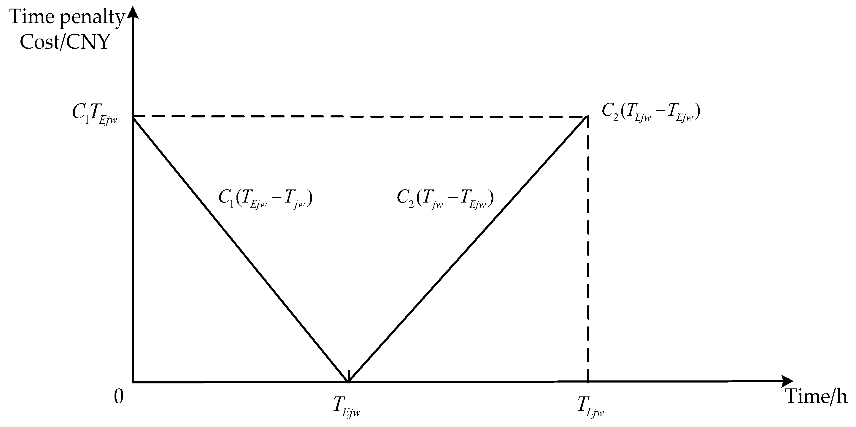
3.2.1. Description of Time Penalty Cost

Maritime emergency rescue is characterized by a strong time-sensitive rescue, so the time-penalty cost function in MEMD-LRP is constructed, and the relationship between time and time-penalty cost is shown in Figure 2, which is consistent with the authors’ previous study [9].

The time penalty cost function expression is:

$$P_{jw}=\left\{\begin{array}{c}{C}_1\left(T_{Ejw}-T_{jw}\right),T_{jw}<T_{Ejw}\\ 0,T_{jw}=T_{Ejw}\\ C_2\left(T_{jw}-T_{Ejw}\right),T_{jw}>T_{Ejw}\end{array},\forall j\in J,w\in W\right.$$

(1)

3.2.2. Description of Time Satisfaction Loss Cost at Accident Point

The upper-level emergency management decision makers face the challenge of balancing the cost of establishing shore-based emergency reserves with the time satisfaction at accident sites. To simplify calculations, time satisfaction is converted into a cost of time satisfaction loss integrated into the upper-level decision-maker’s objectives. In this paper, a linear time satisfaction function is chosen. When a ship $k$ delivers emergency materials of a certain level to accident point $j$ but fails to meet the expected arrival time $T_{Ej\omega }$ at accident point $j$, time satisfaction is reduced at accident point $j$. The greater the deviation from the arrival time $T_{Ej\omega }$ of emergency materials $w$ at accident point $j$, the more significant the reduction in time satisfaction. Furthermore, the cost associated with the loss of time satisfaction at accident point $j$ is tied to the demand for emergency materials at that accident point. The penalty coefficient for the cost of time satisfaction loss at accident point $j$ follows a segmented function corresponding to time satisfaction, with the functional relationship determined to be $\varphi \left(F\left(T_{jw}\right)\right)$ [9].

The expression representing the time satisfaction function of accident point $j$ concerning the arrival time of a certain level of emergency materials is as follows:

$$F\left(T_{jw}\right)=\left\{\begin{array}{l}1,T_{jw}=T_{Ejw}\\ \frac{T_{Ejw}-T_{jw}}{T_{Ejw}},0\le T_{jw}<T_{Ejw}\\ \frac{T_{Ljw}-T_{jw}}{T_{Ljw}-T_{Ejw}},T_{Ejw}<T_{jw}\le T_{Ljw}\\ 0,T_{Ljw}<T_{jw}\end{array}\right.,\forall j\in J,w\in W$$

(2)

The mathematical representation for the penalty coefficient associated with the loss cost of time satisfaction at accident point $j$ is as follows:

$$\varphi \left(F\left(T_{jw}\right)\right)=\left\{\begin{array}{l}0,F\left(T_{jw}\right)=1\\ 1,F\left(T_{jw}\right)=\frac{T_{Ejw}-T_{jw}}{T_{Ejw}},\forall j\in J,w\in W\\ 1,F\left(T_{jw}\right)=\frac{T_{Ljw}-T_{jw}}{T_{Ljw}-T_{Ejw}},\forall j\in J,w\in W\\ +\infty ,F\left(T_{jw}\right)=0\end{array}\right.$$

(3)

The total cost resulting from the lost time satisfaction at accident point $j$ can be expressed as follows:

$${\displaystyle \sum _{i\in I}{\displaystyle \sum _{j\in J}{\displaystyle \sum _{w\in W}{x}_i}}}\varphi \left(F\left(T_{jw}\right)\right)y_{ij}{D}_{jw}$$

(4)

3.2.3. MEMD-LRP Robust Bi-Level Nominal Models

Based on the above assumptions and cost descriptions, the nominal model (denoted as BLNM) for constructing the robust bi-level model of MEMD-LRP is shown below.

(1)

Upper level modeling:

$$\min f_1={\displaystyle \sum _{i\in I}{F}_i}{x}_i+{\displaystyle \sum _{i\in I}{\displaystyle \sum _{j\in J}{\displaystyle \sum _{w\in W}{x}_i}}}\varphi \left(F\left(T_{jw}\right)\right)y_{ij}{D}_{jw}$$

(5)

$$\mathrm{s}.\mathrm{t}. 1\le {\displaystyle \sum _{i\in I}{x}_i}\le I$$

(6)

$$y_{ij}-x_i\le 0,\forall i\in I,j\in J$$

(7)

$$x_i\in \{0,1\}$$

(8)

The goal defined in objective function (5) is to minimize both the construction expenses of emergency reserves and the costs associated with time satisfaction losses at the accident point; constraint (6) restricts the actual count of emergency reserve constructions to not surpass the number of candidate shore-based emergency reserves; constraint (7) enforces that only when selected as an emergency material reserve can materials be transported; constraint (8) represents an upper-level decision variable.

(2)

Lower level modeling:

$$\min f_2={\displaystyle \sum _{i\in I}{\displaystyle \sum _{j\in J}{\displaystyle \sum _{w\in W}{u}_{jw}}}}{D}_{jw}{C}_{ijw}{y}_{ij}+{\displaystyle \sum _{p,q\in B}{\displaystyle \sum _{k\in K}{z}_{pqk}}}{L}_{pq}{S}_k+{\displaystyle \sum _{k\in K}{C}_0}{q}_k+{\displaystyle \sum _{w\in W}{\displaystyle \sum _{i\in I}{\displaystyle \sum _{j\in J}{y}_{ij}}}}{P}_{jw}$$

(9)

$$\mathrm{s}.\mathrm{t}. {\displaystyle \sum _{i\in I}{y}_{ij}}=1,\forall j\in J$$

(10)

$${\displaystyle \sum _{k\in K}{\displaystyle \sum _{j\in J}{z}_{ijk}}}\ge x_i,\forall i\in I$$

(11)

$${\displaystyle \sum _{i\in I}{\displaystyle \sum _{j\in J}{z}_{ijk}}}\le 1,\forall k\in K$$

(12)

$$z_{pqk}\le q_k,\forall p,q\in B,p\ne q,k\in K$$

(13)

$${\displaystyle \sum _{k\in K}{\displaystyle \sum _{p\in B}{z}_{pjk}}}{u}_{jw}=1,\forall j\in J,w\in W$$

(14)

$${\displaystyle \sum _{p,q\in B}{\displaystyle \sum _{i\in I}{\displaystyle \sum _{j\in J}{\displaystyle \sum _{w\in W}{D}_{jw}}}}}{u}_{jw}{y}_{ij}{z}_{pqk}\le G,\forall k\in K$$

(15)

$${\displaystyle \sum _{k\in K}{z}_{pqk}}=0,\forall p,q\in I$$

(16)

$${\displaystyle \sum _{p\in B}{z}_{pqk}}-{\displaystyle \sum _{p\in B}{z}_{qpk}}=0,\forall k\in K,q\in B$$

(17)

$${\displaystyle \sum _{j\in J}{z}_{ijk}}+{\displaystyle \sum _{j\in J}{z}_{jrk}}\le 1,\forall i,r\in I,k\in K$$

(18)

$$y_{ij}{D}_{j(w+1)}\le u_{jw}A,\forall w=1,\cdots ,\left|W\right|-1,i\in I,j\in J$$

(19)

$$T_{jw}\le T_{j(w+1)},\forall w=1,\cdots ,\left|W\right|-1,j\in J$$

(20)

$${\displaystyle \sum _{j\in J}{T}_{jw}}\le {\displaystyle \sum _{j\in J}{T}_{j(w+1)}},\forall w=1,\cdots ,|W|-1,j\in J$$

(21)

$$y_{ij}{T}_{jw}\le T_{Ljw},\forall i\in I,j\in J,w\in W$$

(22)

$$T_{pw}+z_{pqk}{T}_{pq}\le T_{Lqw},\forall p,q\in J,w\in W,z_{pqk}=1$$

(23)

$$y_{ij}\in \{0,1\},q_k\in \{0,1\},z_{pqk}\in \{0,1\}$$

(24)

In a bi-level programming model, the upper model’s constraints apply uniformly to the lower model. Objective function (9) aims to minimize the total costs encompassing different levels of emergency material distribution, ship transportation, ship dispatch, and time penalties; constraint (10) ensures that each incident point receives assistance from a single emergency reserve; constraint (11) ensures that each selected emergency materials reserve is assigned ships; constraint (12) ensures that each ship is linked to one selected emergency reserve; constraint (13) indicates that only operational ships are eligible for transportation; constraint (14) mandates that, during the distribution of each level of emergency materials, only one ship passes through each accident point; constraint (15) indicates that the demand for emergency materials at the accident point along a ship’s route must not exceed the ship’s capacity; constraint (16) indicates that there cannot be transportation between any two emergency materials reserves; constraint (17) indicates that ships entering from a point must also exit from that point; constraint (18) indicates that a ship leaving the emergency reserve is required to return to the same emergency reserve in the end; constraint (19) indicates that the transport of emergency materials from emergency reserve $i$ to accident point $j$ can commence for the next level only after the emergency materials of the previous level have been transported; constraints (20) and (21) denote that the actual delivery time of high-priority emergency materials is strictly less than the actual delivery time of low-priority emergency materials; constraint (22) denotes that the actual arrival time of level $w$ emergency materials transported from emergency material reserve $i$ to incident point $j$ is less than or equal to the latest allowable delivery time for level $w$ emergency materials at incident point $j$; constraint (23) accounts for the time window constraints on a ship while servicing multiple point points, and constraint (24) is the lower-level decision variable.

The time for the ship $k$ to reach the accident point $q$ is calculated by the following formula:

$$T_{qw}=T_{pw}+z_{pqk}{T}_{pq},\forall p,q\in J,w\in W,z_{pqk}=1$$

(25)

The ship’s $k$ speed will be influenced by both the wind and current speed; consequently, the ship’s $k$ actual average speed is the vector superposition of the average still water speed, wind speed, and current speed of the ship $k$, which is calculated as follows:

$$V_{pqk}=V_{pqk}^A+V_1+V_2,\forall p,q\in B,p\ne q$$

(26)

3.2.4. MEMD-LRP Robust Bi-Level Modeling

The upper-level objective function in the MEMD-LRP robust bi-level nominal model is first linearized by introducing the auxiliary variable $CL$, which leads to constraint (27) from constraints (2) and (3):

$$CL=\left\{\begin{array}{c}0,T_{jw}=T_{Ejw}\\ 1,0\le T_{jw}<T_{Ejw} \mathrm{or} T_{Ejw}<T_{jw}\le T_{Ljw},\forall j\in J,w\in W\\ +\infty ,T_{Ljw}<T_{jw}\end{array}\right.$$

(27)

Continuing to linearize the upper objective function by introducing the auxiliary variable $l_{ij}$ and making it equal to the product of two 0–1 variables, we have (28)–(32):

$$l_{ij}=x_i{y}_{ij},\forall i\in I,j\in J$$

(28)

$$l_{ij}\le x_i,\forall i\in I,j\in J$$

(29)

$$l_{ij}\le y_{ij},\forall i\in I,j\in J$$

(30)

$$l_{ij}\ge x_i+y_{ij}-1,\forall i\in I,j\in J$$

(31)

$$l_{ij}\in \{0,1\}$$

(32)

Function (5) is then transformed into function (33):

$$\min f_1={\displaystyle \sum _{i\in I}{F}_i}{x}_i+{\displaystyle \sum _{i\in I}{\displaystyle \sum _{j\in J}{\displaystyle \sum _{w\in W}C}}}L{l}_{ij}{D}_{jw}$$

(33)

In this paper, we consider that the uncertain parameter ship sailing time only appears in the constraints of the lower level, which has no direct influence on the upper and lower objective functions, whereas the uncertain parameter accident point demand for different levels of emergency materials has a direct influence on the upper and lower objective functions and constraints; the two uncertain parameters do not appear in the same constraints at the same time. The robust model proposed by Soyster [37] is optimized for the worst case scenario. Maritime emergency response has urgency and high requirements on rescue time when considering uncertainty in ship sailing time. The conservative Soyster robust model is used to construct a robust bi-level model containing uncertain parameters regarding the ship’s sailing time. The Bertsimas and Sim [38] robust model is a gradual development of the Soyster robust model, introducing the budget of uncertainty (BoU) to regulate the degree of robust conservatism. Bertsimas and Sim’s robust model is used to construct a robust bi-level model of emergency material demand at accident points containing uncertain parameters. The degree of conservatism of the whole robust bi-level model can be adjusted by introducing the uncertain budget of the emergency material demand, and the objective function and constraints of the emergency material demand containing uncertain parameters are transformed using the peer-to-peer transformation method of the Bertsimas and Sim robust model [39,40].

It is assumed that the uncertain ship sailing time ${\tilde{T}}_{pq}$ is perturbed in an interval uncertainty set; the different levels of emergency material requirements at the accident point ${\tilde{D}}_{jw}$ are perturbed in a box uncertainty set, and the decision-maker only knows the upper and lower bounds of the unknown parameters, which are distributed on their respective bounded symmetric intervals, and the distribution information is unknown:

$${\tilde{T}}_{pq}\in \left[T_{pq}-{\widehat{T}}_{pq},T_{pq}+{\widehat{T}}_{pq}\right],\forall p,q\in B,p\ne q$$

(34)

$${\tilde{D}}_{jw}\in \left[D_{jw}-b_{jw}{\widehat{D}}_{jw},D_{jw}+b_{jw}{\widehat{D}}_{jw}\right],\forall j\in J,w\in W$$

(35)

In constraints (34) and (35), $T_{pq}$ represents the nominal value (NV) of the ship’s sailing time between nodes, which is equivalent to the corresponding value in the deterministic model, and ${\widehat{T}}_{pq}\ge 0$ is the amount of time perturbation. $D_{j\omega }$ is the nominal value of the demand for different levels of emergency materials at the accident point, ${\widehat{D}}_{jw}\ge 0$ is the amount of demand perturbation, and $b_{j\omega }$ is a random variable taking values in the interval [0,1] and with an unknown distribution, notated as its uncertainty set $U_1=\left\{b_{jw}\mid {\displaystyle \sum _w{\displaystyle \sum _j{b}_{jw}}}\le {\mathrm{\Gamma }}_1,0\le b_{jw}\le 1,\forall j\in J,w\in W\right\}$. And ${\mathrm{\Gamma }}_1$ is the uncertain budget of demand, controlling the uncertainty level of its uncertainty set, defining the box uncertainty set with the budget. The value of ${\mathrm{\Gamma }}_1$ is related to the decision maker’s preference: If the value of the uncertainty budget is larger, the more conservative the robust model is, the better the robustness of the solution, and the more satisfactory results can be obtained in the worst case scenario. However, if the value of the uncertainty budget is smaller, the less robust it is; however, better results may be obtained in the ideal case. Decision makers can adjust the values according to their preferences to obtain decision methods with different degrees of conservatism to achieve a compromise between optimality and robustness [40].

For the upper and lower bounds of the uncertain budget ${\mathrm{\Gamma }}_1$, it is easy to see that ${\mathrm{\Gamma }}_1\ge 0$, by $\forall b_{jw}\in [0,1]$. By the definition of the uncertain set $U_1$, and constraint (35), we also obtain ${\mathrm{\Gamma }}_1\le \left|J\right|\times \left|W\right|$.

MEMD-LRP Robust Bi-Level Model Based on Ship Sailing Time Uncertainty

(1)

Robust bi-level modeling

Observing that the ship sailing time appears in (23) and (25) in the BLNM, the above equations are adjusted correspondingly when constructing the robust bi-level model to obtain the new robust constraints (60) and (63). The MEMD-LRP robust bi-level model based on the uncertainty of ship sailing time denoted as TRBLM is constructed according to the Soyster robust model as follows:

Upper level modeling:

$$\min f_1={\displaystyle \sum _{i\in I}{F}_i}{x}_i+{\displaystyle \sum _{i\in I}{\displaystyle \sum _{j\in J}{\displaystyle \sum _{w\in W}C}}}L{l}_{ij}{D}_{jw}$$

(36)

$$\mathrm{s}.\mathrm{t}. 1\le {\displaystyle \sum _{i\in I}{x}_i}\le I$$

(37)

$$y_{ij}-x_i\le 0,\forall i\in I,j\in J$$

(38)

$$x_i\in \{0,1\}$$

(39)

$$CL=\left\{\begin{array}{c}0,T_{jw}=T_{Ejw}\\ 1,0\le T_{jw}<T_{Ejw} \mathrm{or} T_{Ejw}<T_{jw}\le T_{Ljw},\forall j\in J,w\in W\\ +\infty ,T_{Ljw}<T_{jw}\end{array}\right.$$

(40)

$$l_{ij}=x_i{y}_{ij},\forall i\in I,j\in J$$

(41)

$$l_{ij}\le x_i,\forall i\in I,j\in J$$

(42)

$$l_{ij}\le y_{ij},\forall i\in I,j\in J$$

(43)

$$l_{ij}\ge x_i+y_{ij}-1,\forall i\in I,j\in J$$

(44)

$$l_{ij}\in \{0,1\}$$

(45)

The objective function and constraints of the TRBLM upper model are changed, except that (37)–(39) are exactly the same as BLNM, but the meaning is exactly the same and will not be repeated.

Lower level modeling:

$$\min f_2={\displaystyle \sum _{i\in I}{\displaystyle \sum _{j\in J}{\displaystyle \sum _{w\in W}{u}_{jw}}}}{D}_{jw}{C}_{ijw}{y}_{ij}+{\displaystyle \sum _{p,q\in B}{\displaystyle \sum _{k\in K}{z}_{pqk}}}{L}_{pq}{S}_k+{\displaystyle \sum _{k\in K}{C}_0}{q}_k+{\displaystyle \sum _{w\in W}{\displaystyle \sum _{i\in I}{\displaystyle \sum _{j\in J}{y}_{ij}}}}{P}_{jw}$$

(46)

$$\mathrm{s}.\mathrm{t}. {\displaystyle \sum _{i\in I}{y}_{ij}}=1,\forall j\in J$$

(47)

$${\displaystyle \sum _{k\in K}{\displaystyle \sum _{j\in J}{z}_{ijk}}}\ge x_i,\forall i\in I$$

(48)

$${\displaystyle \sum _{i\in I}{\displaystyle \sum _{j\in J}{z}_{ijk}}}\le 1,\forall k\in K$$

(49)

$$z_{pqk}\le q_k,\forall p,q\in B,p\ne q,k\in K$$

(50)

$${\displaystyle \sum _{k\in K}{\displaystyle \sum _{p\in B}{z}_{pjk}}}{u}_{jw}=1,\forall j\in J,w\in W$$

(51)

$${\displaystyle \sum _{p,q\in B}{\displaystyle \sum _{i\in I}{\displaystyle \sum _{j\in J}{\displaystyle \sum _{w\in W}{D}_{jw}}}}}{u}_{jw}{y}_{ij}{z}_{pqk}\le G,\forall k\in K$$

(52)

$${\displaystyle \sum _{k\in K}{z}_{pqk}}=0,\forall p,q\in I$$

(53)

$${\displaystyle \sum _{p\in B}{z}_{pqk}}-{\displaystyle \sum _{p\in B}{z}_{qpk}}=0,\forall k\in K,q\in B$$

(54)

$${\displaystyle \sum _{j\in J}{z}_{ijk}}+{\displaystyle \sum _{j\in J}{z}_{jrk}}\le 1,\forall i,r\in I,k\in K$$

(55)

$$y_{ij}{D}_{j(w+1)}\le u_{jw}A,\forall w=1,\cdots ,\left|W\right|-1,i\in I,j\in J$$

(56)

$$T_{jw}\le T_{j(w+1)},\forall w=1,\cdots ,\left|W\right|-1,j\in J$$

(57)

$${\displaystyle \sum _{j\in J}{T}_{jw}}\le {\displaystyle \sum _{j\in J}{T}_{j(w+1)}},\forall w=1,\cdots ,|W|-1,j\in J$$

(58)

$$y_{ij}{T}_{jw}\le T_{Ljw},\forall i\in I,j\in J,w\in W$$

(59)

$$T_{pw}+z_{pqk}{\tilde{T}}_{pq}\le T_{pqw},\forall p,q\in J,w\in W,z_{pqk}=1$$

(60)

$$y_{ij}\in \{0,1\},q_k\in \{0,1\},z_{pqk}\in \{0,1\}$$

(61)

$$V_{pqk}=V_{pqk}^A+V_1+V_2,\forall p,q\in B,p\ne q$$

(62)

where the time for the ship $k$ to reach the accident point $q$ is calculated as:

$$T_{qw}=T_{pw}+z_{pqk}{\tilde{T}}_{pq},\forall p,q\in J,w\in W,z_{pqk}=1$$

(63)

The objective function and constraints of the TRBLM lower model, except for (34) and (35), are identical to those of the BLNM, but have exactly the same meaning and will not be repeated.

(2)

Robust equivalent model

According to references [37,41,42], the transformation of constraint (60) and (63) containing the equals sign yields constraints (64) and (65):

$$T_{pw}+z_{pqk}\left(T_{pq}+{\widehat{T}}_{pq}\right)\le T_{Lqw},\forall p,q\in J,w\in W,z_{pqk}=1$$

(64)

$$z_{pqk}\left(T_{pq}-{\widehat{T}}_{pq}\right)\le T_{qw}-T_{pw}\le z_{pqk}\left(T_{pq}+{\widehat{T}}_{pq}\right),\forall p,q\in J,w\in W,z_{pqk}=1$$

(65)

The robust equivalent model TRBLM-RC of the model TRBLM is obtained:

Upper objective function (36) with constraints (37)–(39) and (40)–(45), and lower objective function (9) with constraints (10)–(22), (24), (26), (64), and (65).

When the amount of time perturbation is ${\widehat{T}}_{pq}=0$, the ship sailing time is equal to the corresponding value in the deterministic case, so the models TRBLM, TRBLM-RC, and BLNM are equivalent.

MEMD-LRP Robust Bi-Level Model Based on the Uncertainty of Emergency Material Demand at Accident Points

(1)

Robust bi-level model

It is observed that the demand for emergency materials at the accident point appears in objective functions (36) and (9), and constraints (15) and (19) of the model. Thus, the above equations must be adjusted correspondingly when constructing the robust optimization model considering the uncertainty of the demand for emergency materials at the accident point to obtain the new robust upper and lower objective functions (66) and (76), and robust constraints (66) and (76).Other constraints are kept unchanged for the time being. Denote the robust bi-level model as DRBLM, as follows:

Upper level modeling:

$$\min f_1=\min \left({\displaystyle \sum _{i\in I}{F}_i}{x}_i+\max {\displaystyle \sum _{i\in I}{\displaystyle \sum _{j\in J}{\displaystyle \sum _{w\in W}\left(D_{jw}+b_{jw}{\widehat{D}}_{jw}\right)}}}CL{l}_{ij}\right)$$

(66)

$$\mathrm{s}.\mathrm{t}. 1\le {\displaystyle \sum _{i\in I}{x}_i}\le I$$

(67)

$$y_{ij}-x_i\le 0,\forall i\in I,j\in J$$

(68)

$$x_i\in \{0,1\}$$

(69)

$$CL=\left\{\begin{array}{c}0,T_{jw}=T_{Ejw}\\ 1,0\le T_{jw}<T_{Ejw} \mathrm{or} T_{Ejw}<T_{jw}\le T_{Ljw},\forall j\in J,w\in W\\ +\infty ,T_{Ljw}<T_{jw}\end{array}\right.$$

(70)

$$l_{ij}=x_i{y}_{ij},\forall i\in I,j\in J$$

(71)

$$l_{ij}\le x_i,\forall i\in I,j\in J$$

(72)

$$l_{ij}\le y_{ij},\forall i\in I,j\in J$$

(73)

$$l_{ij}\ge x_i+y_{ij}-1,\forall i\in I,j\in J$$

(74)

$$l_{ij}\in \{0,1\}$$

(75)

Lower level modeling:

$$\min f_2=\min \left({\displaystyle \sum _{p,q\in B}{\displaystyle \sum _{k\in K}{z}_{pqk}}}{L}_{pq}{S}_k+{\displaystyle \sum _{k\in K}{C}_0}{q}_k+{\displaystyle \sum _{w\in W}{\displaystyle \sum _{i\in I}{\displaystyle \sum _{j\in J}{y}_{ij}}}}{P}_{jw}+\max {\displaystyle \sum _{i\in I}{\displaystyle \sum _{j\in J}{\displaystyle \sum _{w\in W}\left(D_{jw}+b_{jw}{\widehat{D}}_{jw}\right)}}}{u}_{jw}{C}_{ijw}{y}_{ij}\right)$$

(76)

$$\mathrm{s}.\mathrm{t}. {\displaystyle \sum _{i\in I}{y}_{ij}}=1,\forall j\in J$$

(77)

$${\displaystyle \sum _{k\in K}{\displaystyle \sum _{j\in J}{z}_{ijk}}}\ge x_i,\forall i\in I$$

(78)

$${\displaystyle \sum _{i\in I}{\displaystyle \sum _{j\in J}{z}_{ijk}}}\le 1,\forall k\in K$$

(79)

$$z_{pqk}\le q_k,\forall p,q\in B,p\ne q,k\in K$$

(80)

$${\displaystyle \sum _{k\in K}{\displaystyle \sum _{p\in B}{z}_{pjk}}}{u}_{jw}=1,\forall j\in J,w\in W$$

(81)

$${\displaystyle \sum _{k\in K}{z}_{pqk}}=0,\forall p,q\in I$$

(82)

$${\displaystyle \sum _{p\in B}{z}_{pqk}}-{\displaystyle \sum _{p\in B}{z}_{qpk}}=0,\forall k\in K,q\in B$$

(83)

$${\displaystyle \sum _{j\in J}{z}_{ijk}}+{\displaystyle \sum _{j\in J}{z}_{jrk}}\le 1,\forall i,r\in I,k\in K$$

(84)

$$T_{jw}\le T_{j(w+1)},\forall w=1,\cdots ,\left|W\right|-1,j\in J$$

(85)

$${\displaystyle \sum _{j\in J}{T}_{jw}}\le {\displaystyle \sum _{j\in J}{T}_{j(w+1)}},\forall w=1,\cdots ,|W|-1,j\in J$$

(86)

$$y_{ij}{T}_{jw}\le T_{Ljw},\forall i\in I,j\in J,w\in W$$

(87)

$$T_{pw}+z_{pqk}{T}_{pq}\le T_{Lqw},\forall p,q\in J,w\in W,z_{pqk}=1$$

(88)

$$y_{ij}\in \{0,1\},q_k\in \{0,1\},z_{pqk}\in \{0,1\}$$

(89)

$$T_{qw}=T_{pw}+z_{pqk}{T}_{pq},\forall p,q\in J,w\in W,z_{pqk}=1$$

(90)

$$V_{pqk}=V_{pqk}^A+V_1+V_2,\forall p,q\in B,p\ne q$$

(91)

$${\displaystyle \sum _{p,q\in B}{\displaystyle \sum _{i\in I}{\displaystyle \sum _{j\in J}{\displaystyle \sum _{w\in W}{D}_{jw}}}}}{u}_{jw}{y}_{ij}{z}_{pqk}+\max {\displaystyle \sum _{p,q\in B}{\displaystyle \sum _{i\in I}{\displaystyle \sum _{j\in J}{\displaystyle \sum _{w\in W}{b}_{jw}}}}}{\widehat{D}}_{jw}{u}_{jw}{y}_{ij}{z}_{pqk}\le G,\forall k\in K$$

(92)

$$y_{ij}{D}_{j(w+1)}+\max y_{ij}\left(b_{j(w+1)}{\widehat{D}}_{j(w+1)}\right)\le u_{jw}A,\forall i\in I,j\in J,w=1,\cdots ,\left|\mathrm{W}\right|-1$$

(93)

(2)

Robust equivalent model

Upper and lower objective functions (66) and (76) of the DRBLM and constraints (92) and (93) of the DRBLM are nonlinear expressions containing inner maximization subterms, which are not convenient to solve directly. Using strong duality theory, it is possible to transform the DRBLM into a more easily solvable robust equivalent model, denoted as RBLM-RC.

The problem of maximizing the inner level of the objective function (66) is first decomposed to obtain Equation (94):

$${\max }_{b_{jw}\in U_1}{\displaystyle \sum _{i\in I}{\displaystyle \sum _{j\in J}{\displaystyle \sum _{w\in W}\left(D_{jw}+b_{jw}{\widehat{D}}_{jw}\right)}}}CL{l}_{ij}={\displaystyle \sum _{i\in I}{\displaystyle \sum _{j\in J}{\displaystyle \sum _{w\in W}{D}_{jw}}}}CL{l}_{ij}+{\max }_{b_{jw}\in U_1}{\displaystyle \sum _{i\in I}{\displaystyle \sum _{j\in J}{\displaystyle \sum _{w\in W}{b}_{jw}}}}{\widehat{D}}_{jw}CL{l}_{ij}$$

(94)

The linear programming problem with inner-level maximization is shown in constraints (95)–(97):

$${\max }_{b_{jw}\in U_1}{\displaystyle \sum _{i\in I}{\displaystyle \sum _{j\in J}{\displaystyle \sum _{w\in W}{b}_{jw}}}}{\widehat{D}}_{jw}CL{l}_{ij}$$

(95)

$$\mathrm{s}.\mathrm{t}. {\displaystyle \sum _w{\displaystyle \sum _j{b}_{jw}}}\le {\mathrm{\Gamma }}_1$$

(96)

$$0\le b_{jw}\le 1$$

(97)

Transformation according to the strong duality theory further yields duality problems (98)–(100) for problems (95)–(97), where ${\rho }_{jw},\theta$ is a duality variable.

$$\min {\rho }_{jw}+{\mathrm{\Gamma }}_1\theta$$

(98)

$$\mathrm{s}.\mathrm{t}. {\rho }_{jw}+\theta \ge {\displaystyle \sum _{i\in I}{\displaystyle \sum _{j\in J}{\displaystyle \sum _{w\in W}{\widehat{D}}_{jw}}}}CL{l}_{ij},\forall j\in J,w\in W$$

(99)

$${\rho }_{jw},\theta \ge 0$$

(100)

Function (66) is then converted to function (101):

$$\min f_1={\displaystyle \sum _{i\in I}{F}_i}{x}_i+{\displaystyle \sum _{i\in I}{\displaystyle \sum _{j\in J}{\displaystyle \sum _{w\in W}{D}_{jw}}}}CL{l}_{ij}+{\displaystyle \sum _{i\in I}{\displaystyle \sum _{j\in J}{\displaystyle \sum _{w\in W}{\rho }_{jw}}}}+{\mathrm{\Gamma }}_1\theta$$

(101)

Similarly, objective function (41) is then transformed into function (102), which satisfies constraints (103) and (104):

$$\min f_2={\displaystyle \sum _{p,q\in B}{\displaystyle \sum _{k\in K}{z}_{pqk}}}{L}_{pq}{S}_k+{\displaystyle \sum _{k\in K}{C}_0}{q}_k+{\displaystyle \sum _{w\in W}{\displaystyle \sum _{i\in I}{\displaystyle \sum _{j\in J}{y}_{ij}}}}{P}_{jw}+{\displaystyle \sum _{i\in I}{\displaystyle \sum _{j\in J}{\displaystyle \sum _{w\in W}{D}_{jw}}}}{u}_{jw}{C}_{ijw}{y}_{ij}+{\displaystyle \sum _{i\in I}{\displaystyle \sum _{j\in J}{\displaystyle \sum _{w\in W}{\rho }_{jw1}}}}+{\mathrm{\Gamma }}_1{\theta }_1$$

(102)

$$\mathrm{s}.\mathrm{t}. {\rho }_{jw1}+{\theta }_1\ge {\displaystyle \sum _{i\in I}{\displaystyle \sum _{j\in J}{\displaystyle \sum _{w\in W}{\widehat{D}}_{jw}}}}{u}_{jw}{C}_{ijw}{y}_{ij},\forall i\in I,j\in J,w\in W$$

(103)

$${\rho }_{jw1},{\theta }_1\ge 0$$

(104)

The treatment of constraint (66) according to the strong duality theory leads to constraints (103)–(106):

$${\displaystyle \sum _{p,q\in B}{\displaystyle \sum _{i\in I}{\displaystyle \sum _{j\in J}{\displaystyle \sum _{w\in W}{D}_{jw}}}}}{u}_{jw}{y}_{ij}{z}_{pqk}+{\max }_{b_{jw}\in U_1}{\displaystyle \sum _{p,q\in B}{\displaystyle \sum _{i\in I}{\displaystyle \sum _{j\in J}{\displaystyle \sum _{w\in W}{b}_{jw}}}}}{\widehat{D}}_{jw}{u}_{jw}{y}_{ij}{z}_{pqk}\le G,\forall k\in K$$

(105)

$${\displaystyle \sum _{p,q\in B}{\displaystyle \sum _{i\in I}{\displaystyle \sum _{j\in J}{\displaystyle \sum _{w\in W}{D}_{jw}}}}}{u}_{jw}{y}_{ij}{z}_{pqk}+{\min }_{{\rho }_{jw2},{\theta }_2}{\displaystyle \sum _{p,q\in B}{\displaystyle \sum _{i\in I}{\displaystyle \sum _{j\in J}{\displaystyle \sum _{w\in W}{\rho }_{jw2}}}}}+{\mathrm{\Gamma }}_1{\theta }_2\le G,\forall k\in K$$

(106)

$$\mathrm{s}.\mathrm{t}. {\widehat{D}}_{jw}{u}_{jw}{y}_{ij}{z}_{pqk}\le {\rho }_{jw2}+{\theta }_2,\forall i\in I,j\in J,p,q\in B,w\in W$$

(107)

$${\rho }_{jw2},{\theta }_2\ge 0,\forall j\in J,w\in W$$

(108)

where ${\rho }_{jw2}$ and ${\theta }_2$ are duality variables, the “min” sign in constraint (106) can be ignored, and constraint (106) is equivalent to (109).

$${\displaystyle \sum _{p,q\in B}{\displaystyle \sum _{i\in I}{\displaystyle \sum _{j\in J}{\displaystyle \sum _{w\in W}{D}_{jw}}}}}{u}_{jw}{y}_{ij}{z}_{pqk}+{\displaystyle \sum _{p,q\in B}{\displaystyle \sum _{i\in I}{\displaystyle \sum _{j\in J}{\displaystyle \sum _{w\in W}{\rho }_{jw2}}}}}+{\mathrm{\Gamma }}_1{\theta }_2\le G,\forall k\in K$$

(109)

Similarly, constraint (76) can be transformed into (108)–(110):

$$y_{ij}{D}_{j(\mathrm{w}+1)}+{\rho }_{jw3}+{\mathrm{\Gamma }}_1{\theta }_3\le u_{jw}A,\forall i\in I,j\in J,w=1,\cdots ,\left|\mathrm{W}\right|-1$$

(110)

$$\mathrm{s}.\mathrm{t}. y_{ij}{\widehat{D}}_{j(\mathrm{w}+1)}\le {\rho }_{jw3}+{\theta }_3,\forall i\in I,j\in J,w=1,\cdots ,\left|\mathrm{W}\right|-1$$

(111)

$${\rho }_{jw3},{\theta }_3\ge 0,\forall j\in J,w\in W$$

(112)

The robust equivalent model DRBLM-RC of the model DRBLM is obtained:

Upper objective function (101) with constraints (6)–(8), (27)–(32), (99), and (100), and lower objective function (102) with constraints (10)–(14), (16)–(18), (20)–(26), (103), (104) and (107)–(112).

When the demand uncertainty budget is ${\mathrm{\Gamma }}_1=0$, the demand for emergency materials is equal to the corresponding value in the deterministic scenario, so the models DRBLM, DRBLM-RC, and BLNM are equivalent.

3.3. Solution Method

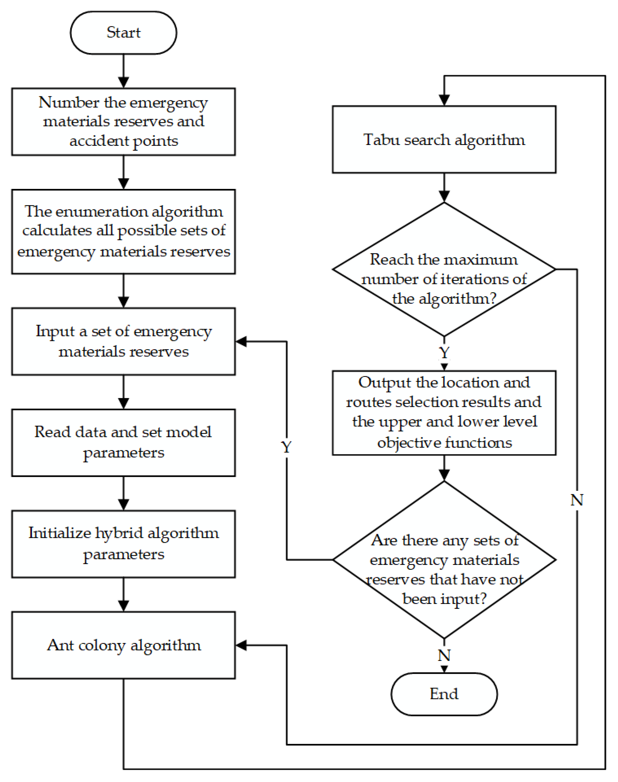
The bi-level programming model is an NP-hard problem, and no exact solution algorithm exists [43]. Whether it is the robust bi-level nominal model constructed in this paper or the transformed robust equivalent model, due to the interaction between the upper level decision and the lower level decision, and many variables and constraints, this makes the solution more and more difficult. The following two algorithms should be combined; the ant colony algorithm, which has a strong global optimization search capability, and the tabu search algorithm, which has a strong local search capability, avoid falling into the local optimum, and obtains the global optimal solution [44,45]. The ACO-TS algorithm designed in this paper is the same as the one previously designed by the authors in the literature [9], except the corresponding parameters are adjusted according to the model when solving, which will not be repeated here. The specific solution flowchart is shown in Figure 3.

4. Solution Analysis

4.1. Example Information

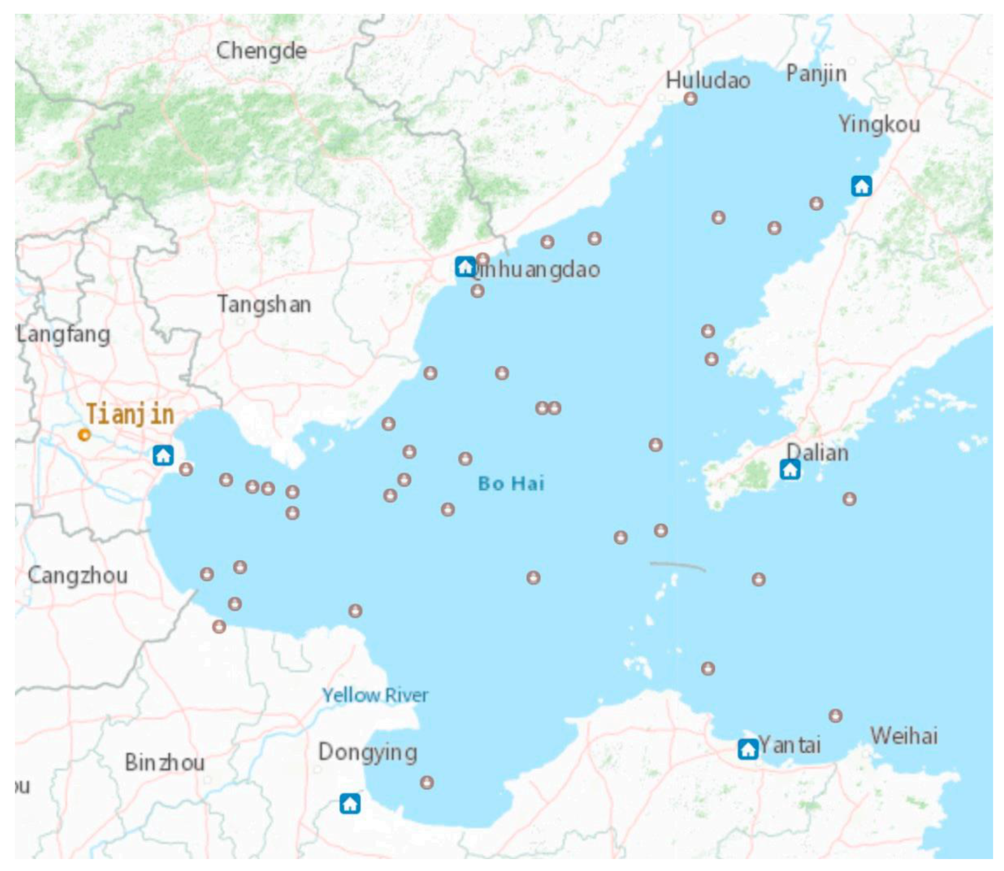
Six ports in the Bohai Sea area were selected as alternative shore-based emergency material reserves, and 40 real historical cases in the Bohai Sea area were selected to design the arithmetic examples of this study according to the accident level, adding the emergency materials of different priority levels as well as the time window of the accident point and other related information. The example information of this paper is the same as that in study [9], which is shown in Appendix A.

The models and algorithms designed in this paper are solved using MATLAB R2017a and run on a computer with Intel(R) Core (TM) i7-10510U CPU @ 1.80 GHz CPU and 16 GB RAM. The key algorithmic parameters include the number of iterations $N$, number of ants $m$, ant crawling speed $speed$, the pheromone evaporation coefficient $\rho$, pheromone increase intensity $Q$, length of the taboo table $L$, and so on.

4.2. Analysis of the Algorithm and Solution Results

4.2.1. Algorithm Analysis

To verify the effectiveness of the algorithm in this paper, we compared the results of the ACO algorithm with the TS algorithm and the ACO algorithm without the TS algorithm in solving the BLNM model. During the experiment, we found that when the parameter is set to $N=150, m=150, \mathrm{speed} =0.05, Q=1$, the ACO algorithm cannot obtain the feasible solution, while the ACO-TS algorithm can obtain the feasible solution. When the parameter is set to $N=1000, m=200, \mathrm{speed} =0.05, Q=1$, ACO can obtain the feasible solution when the number of emergency material reserves is six. We set the parameter to $N=150, m=150, \mathrm{speed} =0.05, Q=1,L=20$, and use the ACO-TS algorithm to obtain the optimal solution under different emergency material reserve quantities, as shown in

Table 3. The optimal solution of the BLNM model obtained by the ACO-TS algorithm.

Reserves	Upper Total Cost (CNY)	Time Satisfaction Loss Cost (CNY)	Lower Total Cost (CNY)	Emergency Materials Distribution Cost (CNY)	Ship Dispatch Cost (CNY)	Shipping Cost (CNY)	Time Penalty Cost (CNY)
(2,3,5)	560,621	621	90,486.35	2494	66,600	14,175.79	7216.56
(2,4,5,6)	760,621	621	90,479.06	2494	67,500	13,200.90	7284.16
(1,2,3,4,5)	96,0621	621	88,139.80	2494	63,000	15,402.78	7243.02
(1,2,3,4,5,6)	1,160,621	621	88,654.75	2494	64,800	14,397.99	6962.76

.

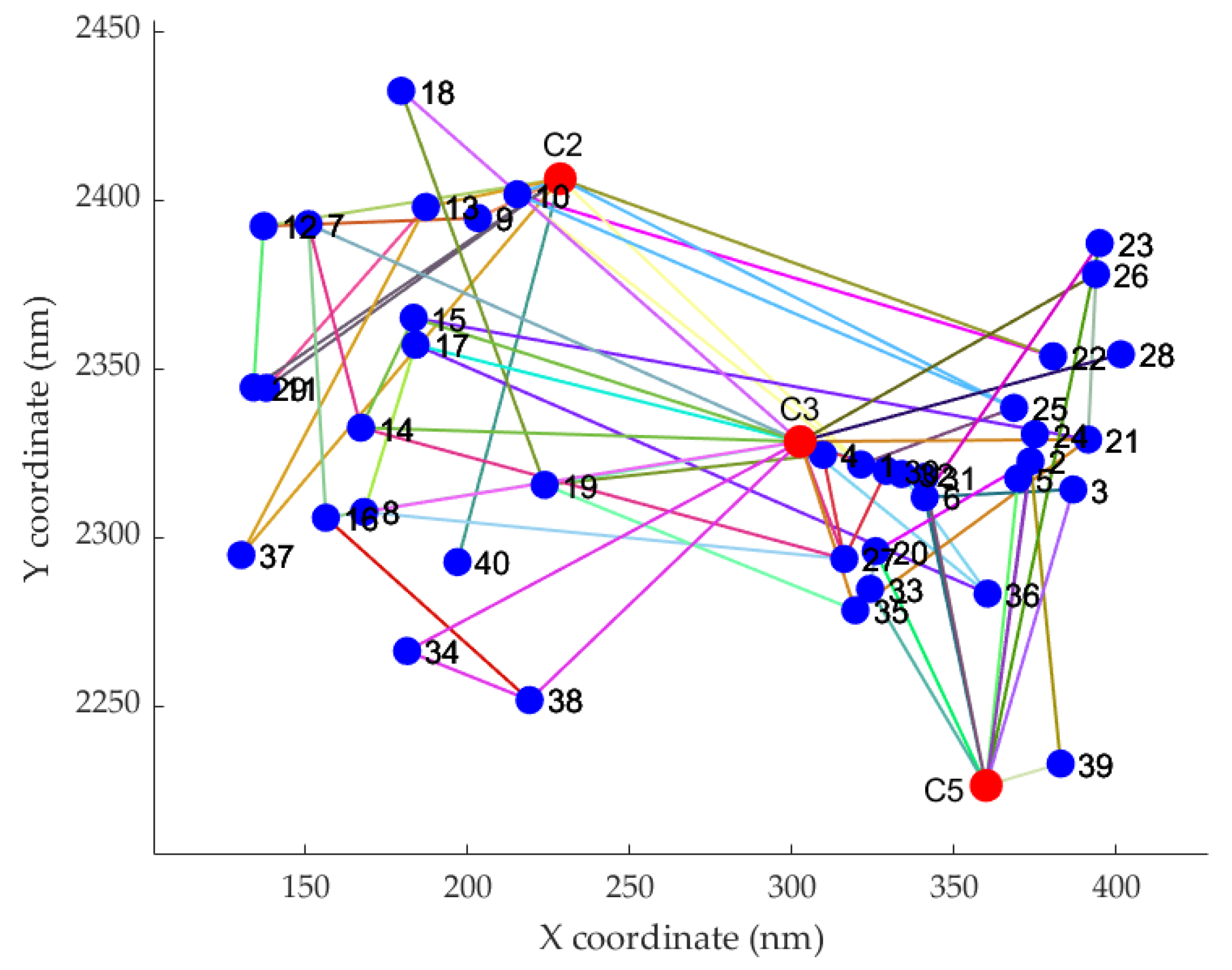
The decision-making process of the bi-level programming model is that the upper level gives priority to the decision-making, and the lower level makes independent decisions based on the upper level’s decision-making, which is fed back to the upper level. Therefore, the solution when the number of emergency material reserves is three is the overall optimal solution of BLNM; that is, to establish emergency materials reserves in Yingkou Port, Tianjin Port, and Weifang Port. The service of all accident points can be satisfied when the total cost of the upper lever is 560,621. Ransikarbum and Mason [46] point out that geographic information system or maps are needed for emergency material distribution location-routing decision aiding; therefore, we used the software to convert the actual geographical coordinates of the emergency materials reserves and the accident points into Cartesian coordinates, and drew the location-routing map in Figure 4, which represents the actual geographical location. The part routes of emergency materials distribution are also shown in

Table 4. Emergency materials distribution route (part).

Reserves	Accident Points of Reserves Service	Ship	Distribution Routes (Emergency Materials Level in Parentheses)
2	1, 9, 10, 11, 12, 13, 17, 22, 25, 29, 37, 40	1	0-37(1)-0
		2	0-11(1)-0
		3	0-1(1)-25(1)-0
		4	0-9(1)-12(1)-0
		5	0-22 (1)-0
		6	0-13(1)-37(2)-0
3	4, 7, 8, 14, 15, 16, 17, 18, 19, 21, 26, 27, 28, 30, 32, 34, 35, 36, 38	1	0-36(1)-17(2)-15(2)-21(3)-0
		2	0-18(1)-19(2)-4(2) -0
		3	0-17(1)-8(1)- 0
		4	0-21(1)-26(1)-0
		5	0-35(1)-19(1)-0
		6	0-27(1)-14(2)-7(3)-0
5	2, 3, 5, 6, 20, 23, 24, 31, 33, 39	1	0-23(1)-0
		2	0-20(1)-2(1)-0
		3	0-39(1)-0
		4	0-3(1)-0
		5	0-24(1)-0
		6	0-33(1)-0

.

It can be seen that the emergency materials reserves have the situation of cross-regional distribution when serving the accident points, and it is not always based on the principle of giving priority to the nearest accident points. This is due to the higher priority and time satisfaction requirements of emergency materials distribution, such as reserve 2 in Figure 4. Table 4 is responsible for the distribution of emergency materials at accident points 22 and 25.

Because our penalty cost function has high requirements for the timely arrival of emergency materials, to further analyze the ACO-TS and ACO algorithms, we increased the parameter of loading and unloading time of emergency materials to $T_k=0.05$ h/unit, and set the algorithm parameter as $N=200, m=200, \mathrm{speed} =0.05, Q=1$ to solve the problem. Equations (23) and (25) are transformed into:

$$T_{pw}+T_k{D}_{pw}{z}_{pqk}+T_{pq}\le T_{Lqw},\forall p,q\in J,w\in W,z_{pqk}=1$$

(113)

$$T_{qw}=T_{pw}+T_k{D}_{pw}{z}_{pqk}+z_{pqk}{T}_{pq},\forall p,q\in J,w\in W,z_{pqk}=1$$

(114)

We have obtained the optimal solution of the two algorithms under different emergency material reserve construction numbers, as shown in

Table 5. The optimal solution of the BLNM model obtained by the ACO-TS algorithm.

Reserves	Upper Total Cost (CNY)	Time Satisfaction Loss Cost (CNY)	Lower Total Cost (CNY)	Emergency Materials Distribution Cost (CNY)	Ship Dispatch Cost (CNY)	Shipping Cost (CNY)	Time Penalty Cost (CNY)
(2,5)	360,621	621	89,078.47	2494	64,800	14,454.11	7330.37
(2,5,6)	560,621	621	91,609.56	2494	66,600	15,306.08	7209.48
(1,2,4,5)	760,621	621	86,400.66	2494	65,700	11,334.81	6871.74
(1,2,3,4,5)	960,621	621	85,884.94	2494	64,800	11,531.14	7059.79
(1,2,3,4,5,6)	1,160,621	621	84,288.8	2494	62,100	12,569.88	7124.91

and

Table 6. The optimal solution of BLNM model obtained by ACO algorithm.

Reserves	Upper Total Cost (CNY)	Time Satisfaction Loss Cost (CNY)	Lower Total Cost (CNY)	Emergency Materials Distribution Cost (CNY)	Ship Dispatch Cost (CNY)	Shipping Cost (CNY)	Time Penalty Cost (CNY)
(1,2,4)	580,621	621	99,227.50	2494	75,600	13,256.34	7877.16
(1,2,3,5,6)	960,621	621	103,418.47	2494	80,100	12,910.56	7913.90
(1,2,3,4,5,6)	1,160,621	621	87,991.54	2494	63,900	14,046.92	7550.63

. When the number of emergency materials reserves constructed is one, neither of the two algorithms has an optimal solution. However, ACO-TS provides optimal solutions as the number of emergency supply depots increases from two to six, while the ACO algorithm only achieves optimal solutions when the number of reserves is three, five, and six. Furthermore, for the same number of emergency materials reserves constructions, ACO-TS yields a smaller optimal solution than ACO.

It takes 64 times to run the algorithm through all emergency materials reserves, but there is no obvious rule in the number of iterations of the algorithm in each operation. To sum up, ACO-TS performs well in solving the problem, and can obtain more feasible solutions and optimal solutions, and the optimal solution is smaller than the corresponding optimal solution of the ACO algorithm.

4.2.2. Solution Results Analysis

To explore the impact of the uncertainty of ship sailing time on MEMD-LRP decision making in the planning period, examples with different values of the time disturbance ratio are set up. To explore the impact of the uncertainty of the demand for emergency materials at the accident point on the MEMD-LRP decision in the planning period, several sets of examples are set up, with different values for the demand uncertainty budget parameter ${\mathrm{\Gamma }}_1$ and demand disturbance ratio. To verify the validity of the model constructed in this paper, the above arithmetic example is solved based on the ACO-TS algorithm described in detail in the literature [9], in which the number of algorithmic iterations $N$ and number of ants $m$ are set to 150, aiming at giving the optimal decision in different cases while exploring the influence of uncertain ship sailing times and uncertain emergency material demand at the accident point on the decision of MEMD-LRP.

1.

The impact of ship sailing time uncertainty on MEMD-LRP decision making

To analyze the effect of uncertain ship sailing time on the MEMD-LRP decisions during the planning period, the model TRBLM-RC is solved using the ACO-TS algorithm, with the time disturbance ratios set to 0, 10%, 20%, 30%, 40%, and 50%. The optimal decision when the time disturbance ratio is equal to 0 is also equivalent to the optimal decision of the nominal model. Based on the decision-making principle that the upper level of bi-level programming prioritizes decision-making, and the lower level makes autonomous decisions on this basis, the optimal location-routing decisions under different time disturbance ratios are obtained. The results are shown in Table 3, and the cost curves under different time disturbance ratios are shown in Figure 4.

From the calculation results presented in

Table 7. The optimal location-routing decision under different time disturbance ratios.

Disturbance Ratio (%)	Location Decisions	Upper Total Cost/CNY	Lower Total Cost/CNY	Total Cost/CNY
0	(2,3,5)	560,621	90,486.35	651,107.35
10	(2,5,6)	560,621	91,645.96	652,266.96
20	(1,2,5)	560,621	96,984.13	657,605.13
30	(2,5,6)	560,621	93,874.88	654,495.88
40	(2,5,6)	560,621	93,984.37	654,605.37
50	(2,3,5)	560,621	94,678.47	655,297.47

and illustrated in Figure 5, the following conclusions can be drawn:

(a)

The optimal number of locations under different time perturbation ratios is the same—both are three—and the total cost of the upper level is the same, but the location results are different. It shows that different time disturbance ratios have a certain influence on the location scheme. The reason why the location results are different, but the total cost of the upper level is the same, is that the decision-maker of the upper level has the right to prioritize decision making and usually chooses the decision that maximizes its interests, so the location decision of the upper level always chooses the case where the total cost of the upper level is the smallest.

(b)

With the upper level total cost remaining the same, the general trend in the lower-level total cost is to increase as the time disruption ratio increases. As the time disturbance ratio increases, the change in ship sailing time gradually increases, and the lower-level decision maker is affected in planning the route. When the disturbance ratio is 0 and 50%, the total cost of the lower-level increases by 4%, although the upper-level location decision is the same. When the disturbance ratios are 10%, 30%, and 40%, the upper-level decisions remain the same, but the total lower-level cost increases by about 2% for the latter two, indicating that the disturbance ratios do have an impact on route planning. When the disturbance ratio is 20%, the lower-level total cost exceeds the lower-level total cost under other disturbance ratios. This is because the lower decision maker is making decisions within the allowable range of the upper decision-maker; the upper decision maker prioritized to make the decision that is most beneficial to him/herself; and the impact of the lower decision-maker for the total cost of the system is less than the upper decision-maker. This kind of decision maker for the lower decision maker may not be the optimal decision, and at this time, the upper decision maker of the location scheme is different from the location scheme under all other perturbation ratios.

(c)

Among the optimal solutions under different time disruption ratios, the choice of location (2,5,6) is the preferred selection. This suggests that establishing emergency materials reserves in Yingkou Port, Weifang Port, and Yantai Port is a more cost-effective option while ensuring the rescue of all accident points.

Through the above analysis, it can be found that the greater the uncertainty of ship sailing time—in most cases to distribute the emergency materials to the accident point in time under constraints such as meeting the time—the greater the total cost of the system, and the greater the cost of emergency rescue. By setting different time perturbation ratios, the upper- and lower-level decision makers can obtain the optimal decision that meets the interests under different sailing time conditions.

2.

The impact of uncertain emergency material demands at accident points on MEMD-LRP decision making

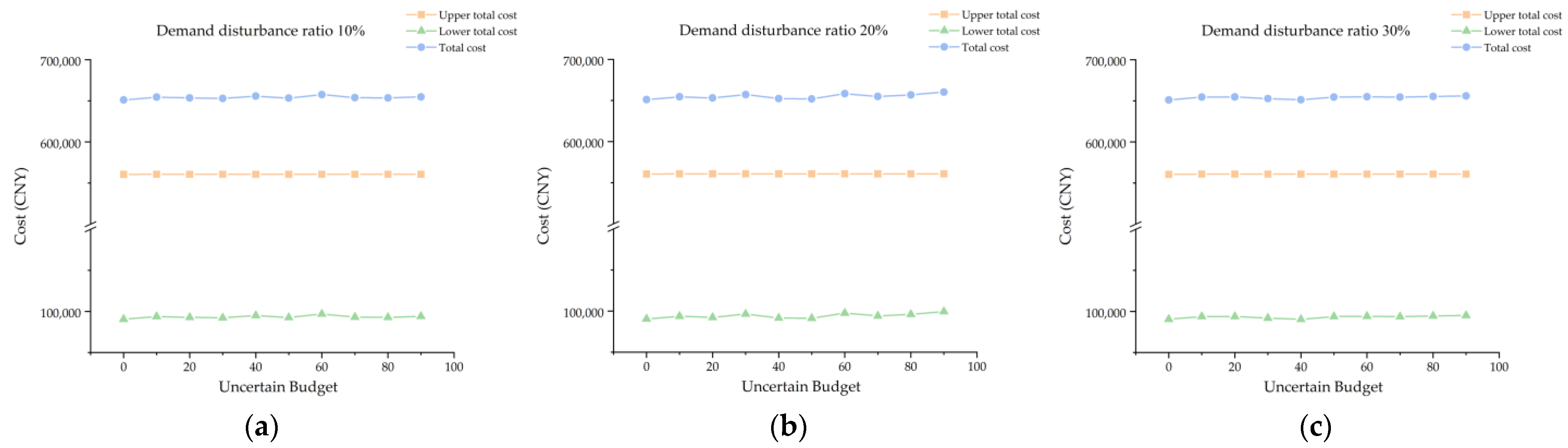
To analyze the impact of the emergency material demands of the uncertain accident points on MEMD-LRP decision making in the planning period, the ACO-TS algorithm is used to solve the DRBLM-RC model. The uncertain budget parameters ${\mathrm{\Gamma }}_1$ are 10, 20, 30, 30, 50, 60, 70, 80, and 90, and the ratio of demand disturbance is 10, 20, and 30. Based on the upper-level priority decision making of bi-level programming and the decision-making principle of lower-level independent decision making, the optimal location-routing decision under different uncertain budgets and different demand disturbance ratios is obtained. The results are shown in

Table 8. The optimal location-routing decision under an uncertain budget and demand disturbance ratios.

Uncertain Budget	Demand Disturbance Ratio (%)	Location Decision	Upper Total Cost/CNY	Lower Total Cost/CNY	Total Cost/CNY
0	—	(2,3,5)	560,621	90,486.35	651,107.35
10	10	(1,2,5)	560,731	93,824.81	654,555.81
	20	(2,5,6)	560,791	93,759.10	654,550.10
	30	(1,2,5)	560,862	93,825.91	654,687.91
20	10	(2,5,6)	560,731	92,874.87	653,605.87
	20	(2,3,5)	560,791	92,301.58	653,092.58
	30	(2,4,5)	560,862	93,864.90	654,726.90
30	10	(2,5,6)	560,731	92,207.50	652,938.50
	20	(2,3,5)	560,791	96,484.78	657,275.78
	30	(1,2,5)	560,862	91,934.91	652,796.91
40	10	(2,5,6)	560,731	95,037.06	655,768.06
	20	(2,3,5)	560,791	91,663.90	652,454.90
	30	(1,2,5)	560,862	90,440.81	651,302.81
50	10	(2,5,6)	560,731	92,591.82	653,322.82
	20	(2,3,5)	560,791	91,275.81	652,066.81
	30	(1,2,5)	560,862	93,825.91	654,687.91
60	10	(1,2,5)	560,731	96,893.24	657,624.24
	20	(2,3,5)	560,791	97,588.78	658,379.78
	30	(2,4,5)	560,862	94,175.60	655,037.60
70	10	(1,2,5)	560,731	93,165.67	653,896.67
	20	(2,5,6)	560,791	94,173.81	654,964.81
	30	(2,4,5)	560,862	93,675.75	654,537.76
80	10	(1,2,5)	560,731	92,870.09	653,601.07
	20	(1,2,5)	560,791	96,044.88	656,835.88
	30	(1,2,5)	560,862	94,448.07	655,310.07
90	10	(2,5,6)	560,731	94,072.70	654,803.70
	20	(2,5,6)	560,791	99,535.75	660,326.75
	30	(2,5,6)	560,862	95,048.72	655,910.72

, and the results under different demand disturbance ratios are shown in Figure 6.

The following conclusions can be drawn from the computational results in Table 8 and Figure 6:

(a)

When uncertain budget and demand-disruption ratios vary, the upper-level reserve locations remain constant at three, but the chosen location schemes differ, indicating a certain influence of uncertain budget and demand-disruption ratios on location selection. When the uncertain budget remains constant, the total upper-level cost exhibits a systematic increase with varying demand-disruption ratios. The reason for the increase in upper-level cost with increasing demand-disruption ratios lies in the fact that the cost of accident point time satisfaction loss in the upper-level objective function is demand-related. Whether in the DRBLM model or the DRBLM-RC model, the values of dual variables depend on the magnitude of demand-disruption. At this time, the impact of uncertain budget values on the upper-level objective function is relatively minimal.

(b)

Once upper-level location decisions are determined, lower-level decision makers make decisions to maximize their interests based on these upper-level decisions. At this stage, the total lower-level cost is influenced by variations in uncertain budget and demand-disruption ratios. In cases where the uncertain budget equals 10, 20, 50, 70, 80, and 90, the overall trend of the total lower-level cost follows an increasing pattern with increasing demand-disruption ratios, but fluctuations occur in these scenarios. However, in cases where the uncertain budget equals 30, 40, and 60, this trend does not hold. In these instances, lower-level decision makers are constrained by the upper-level decisions, where the upper level prioritizes its maximization of interests. As a result, the total lower-level cost for scenarios with lower demand-disruption ratios can exceed that of scenarios with higher demand-disruption ratios. This phenomenon also explains the presence of fluctuations in cases with uncertain budgets of 10, 20, 50, and 90. When demand-disruption ratios are equal, the overall trend of the lower-level total cost generally increases with the increase of an uncertain budget.

(c)

When the demand disturbance ratio is 10% and 20%, this change is not obvious when the demand ratio is 30%, and there are more volatility points. When uncertain budgets are smaller, the changing pattern is less distinct than when uncertain budgets are larger. This illustrates that greater demand uncertainty has a more substantial impact on location-routing decisions. The less distinct or irregular changing patterns can be attributed, on the one hand, to the upper-level’s prioritization of minimizing the overall system cost at the expense of the lower-level’s interests. On the other hand, it could also result from excessively small demand-disruption ratios, causing the influence of uncertain budget on location-routing decisions to be less pronounced.

(d)

Among all the optimal decisions mentioned above, location decisions (1,2,5) and (2,5,6) perform well, and are the preferred choices among numerous decisions; namely, establishing emergency material depots in Dalian Port, Yingkou Port, and Weifang Port, or Yingkou Port, Weifang Port, and Yantai Port. They exhibit resilience against uncertain factors.

Through the analysis presented above, it is evident that both the uncertain demand budget and demand disruption ratio impact the decisions of MEMD-LRP, but this impact heavily relies on their respective values. Decision makers can integrate the circumstances of maritime emergencies, adjusting the values of the uncertain demand budget parameter to subsequently fine-tune the model’s robustness level. With consideration of their preferences, decision makers can flexibly make choices and devise emergency material reserve location and distribution plans, which can effectively address uncertainties in maritime emergencies and enable rapid responses.

5. Conclusions

Taking maritime emergency material distribution as the background, this paper explores the robust bi-level models of MEMD-LRP in uncertain decision-making environments from the perspective of joint decision making among multiple decision makers. Using a case study based on the Bohai Sea area, the research analyzes the optimal decision making of MEMD-LRP under conditions of uncertain sailing time and uncertain emergency material demand at accident points during the planning period. We have solved the problems raised in the introduction; under the constraints of the rescue time window and the priority of emergency materials allocation, a series of emergency material reserve locations and emergency material distribution schemes which can effectively deal with the uncertainty in maritime emergencies are developed for the upper and lower levels of decision makers. The optimal decision under different conditions can not only meet the needs of the accident point, but also reduce the total cost of the emergency logistics system within the prescribed rescue time window, thus realizing the overall optimization of the maritime emergency logistics system. The study yields the following managerial insights:

(a)

Upper-level decision makers such as emergency management departments must possess prioritized decision-making authority. Their goal should be to maximize their own interests while considering the interests of lower-level decision-makers, such as commercial rescue units. When making decisions regarding the selection of emergency material reserve locations, it is necessary not only to evaluate the suitability of the number of reserve constructions but also to consider the feedback from commercial rescue units regarding the location decisions. For lower-level decision makers like commercial rescue units operating within the framework permitted by the emergency management department, these units should make decisions while fully considering their interests. Additionally, they should provide timely feedback on shipping route decisions to the emergency management department.

(b)

Both uncertain ship sailing times and uncertain emergency material demands will influence the decisions of MEMD-LRP, and these decisions will be constrained by the managerial insights mentioned in (a). Upper- and lower-level decision makers can adjust the ratios of ship sailing time disruption and demand disruption, modify the values of the demand uncertainty budget parameter based on maritime emergencies, and make flexible decisions according to their preferences. By doing so, they can formulate emergency material reserve location and emergency material distribution decisions that not only address the uncertainties in maritime emergencies, but also respond rapidly.

(c)

From the perspective of joint decision making among multiple decision makers, this study focuses on two crucial aspects of the maritime emergency logistics system under uncertain conditions: the selection of emergency material reserve locations and the planning of emergency material distribution routes. The aim is to ensure their mutual coordination, which can yield significant benefits in terms of achieving comprehensive decision making and enhancing decision adaptability. This study contributes to a more optimized and flexible emergency logistics system, ultimately improving the capability to respond to maritime emergencies.

This study discusses the impact of uncertain sailing times and uncertain emergency material demand at the accident point on decision maker choices. In the future, we can explore the impact of both on decision-makers simultaneously. In this study, the limited reserve capacity of emergency materials is not considered. In fact, the capacity of different emergency materials in different emergency material reserves may be limited, and the decision making in the case of limited capacity can be discussed in the future. Furthermore, this study did not account for the potential drift of accident points. In reality, maritime emergencies can lead to the drift of accident points due to the intricate marine environment, resulting in shifts in their geographical coordinates. Subsequent research could be undertaken to address the possibility of such accident point drift scenarios. The impact of uncertain delivery times, transportation costs, feasibility probability of transportation routes, and a combination of these factors on MEMD-LRP decision making can also be considered. More importantly, subsequent research will place a stronger emphasis on presenting practical viewpoints and exploring relevant issues in emergency rescue operations under an egalitarian policy framework.

References

- Review of Maritime Transport 2022. Available online: https://unctad.org/rmt2022 (accessed on 22 August 2023).
- Annual Overview of Marine Casualties and Incidents. 2022. Available online: https://safety4sea.com/emsa-annual-overview-of-marine-casualties-and-incidents-2022/ (accessed on 22 August 2023).
- Annual Report. 2022. Available online: https://www.bsu-bund.de/SharedDocs/pdf/EN/Annual_Statistics/Annual_Report_2022.pdf?__blob=publicationFile&v=1 (accessed on 22 August 2023).
- Statistical Bulletin on the Development of Transportation Industry in 2022. Available online: https://xxgk.mot.gov.cn/2020/jigou/zhghs/202306/t20230615_3847023.html (accessed on 22 August 2023).
- Ransikarbum, K.; Mason, S.J. A bi-objective optimisation of post-disaster relief distribution and short-term network restoration using hybrid NSGA-II algorithm. Int. J. Prod. Econ. 2022, 60, 5769–5793. [Google Scholar] [CrossRef]
- Yan, T.; Lu, F.; Wang, S.; Wang, L.; Bi, H. A hybrid metaheuristic algorithm for the multi-objective location-routing problem in the early post-disaster stage. J. Ind. Manag. Optim. 2023, 19, 4663–4691. [Google Scholar] [CrossRef]
- Qin, J.; Ye, Y.; Cheng, B.-R.; Zhao, X.; Ni, L. The Emergency Vehicle Routing Problem with Uncertain Demand under Sustainability Environments. Sustainability 2017, 9, 288. [Google Scholar] [CrossRef]
- Tan, K.; Liu, W.; Xu, F.; Li, C. Optimization Model and Algorithm of Logistics Vehicle Routing Problem under Major Emergency. Mathematics 2023, 11, 1274. [Google Scholar] [CrossRef]
- Peng, Z.; Wang, C.; Xu, W.; Zhang, J. Research on Location-Routing Problem of Maritime Emergency Materials Distribution Based on Bi-Level Programming. Mathematics 2022, 10, 1243. [Google Scholar] [CrossRef]
- Laporte, G.; Nobert, Y. An exact algorithm for minimizing routing and operating costs in depot location. Eur. J. Oper. Res. 1981, 6, 224–226. [Google Scholar] [CrossRef]
- Yang, J.; Sun, H. Battery swap station location-routing problem with capacitated electric vehicles. Comput. Oper. Res. 2015, 55, 217–232. [Google Scholar] [CrossRef]
- Boccia, M.; Crainic, T.G.; Sforza, A.; Sterle, C. Multi-commodity location-routing: Flow intercepting formulation and branch-and-cut algorithm. Comput. Oper. Res. 2018, 89, 94–112. [Google Scholar] [CrossRef]
- Yu, X.; Zhou, Y.; Liu, X.-F. A novel hybrid genetic algorithm for the location routing problem with tight capacity constraints. Appl. Soft. Comput. 2019, 85, 105760. [Google Scholar] [CrossRef]
- Lu, F.; Chen, W.; Feng, W.; Bi, H. 4PL routing problem using hybrid beetle swarm optimization. Soft Comput. 2023, 27, 17011–17024. [Google Scholar] [CrossRef]
- Lu, F.; Feng, W.; Gao, M.; Bi, H.; Wang, S. Corrigendum to “The Fourth-Party Logistics Routing Problem Using Ant Colony System-Improved Grey Wolf Optimization”. J. Adv. Transp. 2022, 2022, 9864064. [Google Scholar] [CrossRef]
- Şatir Akpunar, Ö.; Akpinar, Ş. A hybrid adaptive large neighbourhood search algorithm for the capacitated location routing problem. Expert Syst. Appl. 2021, 168, 114304. [Google Scholar]
- Alamatsaz, K.; Ahmadi, A.; Mirzapour Al-e-hashem, S.M.J. A multiobjective model for the green capacitated location-routing problem considering drivers’ satisfaction and time window with uncertain demand. Environ. Sci. Pollut. Res. 2022, 29, 5052–5071. [Google Scholar] [CrossRef]
- Gan, X.; Liu, J. A multi-objective evolutionary algorithm for emergency logistics scheduling in large-scale disaster relief. In Proceedings of the 2017 IEEE Congress on Evolutionary Computation (CEC), Donostia, Spain, 5–8 June 2017; pp. 51–58. [Google Scholar]
- Liu, C.; Kou, G.; Peng, Y.; Alsaadi, F.E. Location-Routing Problem for Relief Distribution in the Early Post-Earthquake Stage from the Perspective of Fairness. Sustainability 2019, 11, 3420. [Google Scholar] [CrossRef]
- Ai, Y.-f.; Lu, J.; Zhang, L.-L. The optimization model for the location of maritime emergency supplies reserve bases and the configuration of salvage vessels. Transp. Res. E-Log. 2015, 83, 170–188. [Google Scholar] [CrossRef]
- Zhang, B.; Li, H.; Li, S.; Peng, J. Sustainable multi-depot emergency facilities location-routing problem with uncertain information. Appl. Math. Comput. 2018, 333, 506–520. [Google Scholar]
- Afshar, A.; Haghani, A. Modeling integrated supply chain logistics in real-time large-scale disaster relief operations. Socio-Econ. Plan. Sci. 2012, 46, 327–338. [Google Scholar] [CrossRef]
- Zhang, Y.; Qi, M.; Lin, W.-H.; Miao, L. A metaheuristic approach to the reliable location routing problem under disruptions. Transp. Res. E-Log. 2015, 83, 90–110. [Google Scholar] [CrossRef]
- Ghasemi, P.; Khalili-Damghani, K.; Hafezalkotob, A.; Raissi, S. Uncertain multi-objective multi-commodity multi-period multi-vehicle location-allocation model for earthquake evacuation planning. Appl. Math. Comput. 2019, 350, 105–132. [Google Scholar]
- Long, S.; Zhang, D.; Liang, Y.; Li, S.; Chen, W. Robust Optimization of the Multi-Objective Multi-Period Location-Routing Problem for Epidemic Logistics System With Uncertain Demand. IEEE Access 2021, 9, 151912–151930. [Google Scholar] [CrossRef]
- Caunhye, A.M.; Zhang, Y.; Li, M.; Nie, X. A location-routing model for prepositioning and distributing emergency supplies. Transp. Res. E-Log. 2016, 90, 161–176. [Google Scholar] [CrossRef]
- Wang, H.; Du, L.; Ma, S. Multi-objective open location-routing model with split delivery for optimized relief distribution in post-earthquake. Transp. Res. E-Log. 2014, 69, 160–179. [Google Scholar] [CrossRef]
- Raeisi, D.; Jafarzadeh Ghoushchi, S. A robust fuzzy multi-objective location-routing problem for hazardous waste under uncertain conditions. Appl. Intell. 2022, 52, 13435–13455. [Google Scholar] [CrossRef] [PubMed]
- Shen, L.; Tao, F.; Shi, Y.; Qin, R. Optimization of location-routing problem in emergency logistics considering carbon emissions. Int. J. Environ. Res. Public Health 2019, 16, 2982. [Google Scholar] [CrossRef] [PubMed]
- Zhang, L.; Lu, J.; Yang, Z. Dynamic optimization of emergency resource scheduling in a large-scale maritime oil spill accident. Comput. Ind. Eng. 2021, 152, 107028. [Google Scholar] [CrossRef]
- Ghasemi, P.; Goodarzian, F.; Abraham, A. A new humanitarian relief logistic network for multi-objective optimization under stochastic programming. Appl. Intell. 2022, 52, 13729–13762. [Google Scholar] [CrossRef]
- Saeidi-Mobarakeh, Z.; Tavakkoli-Moghaddam, R.; Navabakhsh, M.; Amoozad-Khalili, H. A bi-level and robust optimization-based framework for a hazardous waste management problem: A real-world application. J. Clean Prod. 2020, 252, 119830. [Google Scholar]
- Zhou, Y.; Zheng, B.; Su, J.; Li, Y. The joint location-transportation model based on grey bi-level programming for early post-earthquake relief. J. Ind. Manag. Optim. 2022, 18, 45–73. [Google Scholar] [CrossRef]
- Chen, Y.; Zheng, W.; Li, W.; Huang, Y. The Robustness and Sustainability of Port Logistics Systems for Emergency Supplies from Overseas. J. Adv. Transp. 2020, 2020, 8868533. [Google Scholar] [CrossRef]
- Wei, X.; Qiu, H.; Wang, D.; Duan, J.; Wang, Y.; Cheng, T.C.E. An integrated location-routing problem with post-disaster relief distribution. Comput. Ind. Eng. 2020, 147, 106632. [Google Scholar] [CrossRef]
- Ai, Y.; Zhang, Q. Optimization on cooperative government and enterprise supplies repertories for maritime emergency: A study case in China. Adv. Mech. Eng. 2019, 11, 1687814019828576. [Google Scholar] [CrossRef]
- Soyster, A.L. Technical Note—Convex programming with set-inclusive constraints and applications to inexact linear programming. Oper. Res. 1973, 21, 1154–1157. [Google Scholar] [CrossRef]
- Bertsimas, D.; Sim, M. The price of robustness. Oper. Res. 2004, 52, 35–53. [Google Scholar] [CrossRef]
- Zhou, Y.; Yu, H.; Li, Z.; Su, J.; Liu, C. Robust Optimization of a Distribution Network Location-Routing Problem Under Carbon Trading Policies. IEEE Access 2020, 8, 46288–46306. [Google Scholar] [CrossRef]
- Cheng, X.; Jin, C.; Yao, Q.; Wang, C. Research on Robust Optimization for Route Selection Problem in Multimodal Transportation under the Cap and Trade Policy. Chin. J. Manag. Sci. 2021, 29, 82–90. [Google Scholar]
- Peng, C.; Li, J.; Ran, L.; Wang, S. Emergency Medical Service Station Robust Location Model and Algorithm Under Demand Uncertainty. Oper. Res. Manag. Sci. 2017, 26, 21–28. [Google Scholar]
- Hatefi, S.M.; Jolai, F. Robust and reliable forward–reverse logistics network design under demand uncertainty and facility disruptions. Appl. Math. Model. 2014, 38, 2630–2647. [Google Scholar] [CrossRef]
- Xu, J.P.; Wang, Z.Q.; Zhang, M.X.; Tu, Y. A new model for a 72-h post-earthquake emergency logistics location-routing problem under a random fuzzy environment. Transp. Lett. 2016, 8, 270–285. [Google Scholar] [CrossRef]
- Chen, J.; Gui, P.; Ding, T.; Na, S.; Zhou, Y. Optimization of Transportation Routing Problem for Fresh Food by Improved Ant Colony Algorithm Based on Tabu Search. Sustainability 2019, 11, 6584. [Google Scholar] [CrossRef]
- Li, Q.; Tu, W.; Zhuo, L. Reliable rescue routing optimization for urban emergency logistics under travel time uncertainty. ISPRS Int. J. Geo.-Inf. 2018, 7, 77. [Google Scholar] [CrossRef]
- Ransikarbum, K.; Mason, S.J. Goal programming-based post-disaster decision making for integrated relief distribution and early-stage network restoration. Int. J. Prod. Econ. 2016, 182, 324–341. [Google Scholar] [CrossRef]
Figure 1.
Schematic diagram of the maritime emergency logistics system involving multi-level decision-making agents.
Figure 2.
Time penalty cost curve.
Figure 3.
Flowchart for solving.
Figure 4.
Location-routing map. The red dots represent the selected emergency materials reserves. The blue dots represent the potential accident points. The lines represent the route of the ship.
Figure 5.
Cost profiles for different time perturbation ratios.
Figure 6.
Cost curves for different demand-disruption ratios. (a) The demand disturbance ratio is 10%. (b) Demand disturbance ratio is 20%. (c) Demand disturbance ratio is 30%.