Optimization Based Methods for Solving the Equilibrium Problems with Applications in Variational Inequality Problems and Solution of Nash Equilibrium Models

Abstract

In this paper, we propose two modified two-step proximal methods that are formed through the proximal-like mapping and inertial effect for solving two classes of equilibrium problems. A weak convergence theorem for the first method and the strong convergence result of the second method are well established based on the mild condition on a bifunction. Such methods have the advantage of not involving any line search procedure or any knowledge of the Lipschitz-type constants of the bifunction. One practical reason is that the stepsize involving in these methods is updated based on some previous iterations or uses a stepsize sequence that is non-summable. We consider the well-known Nash–Cournot equilibrium models to support our well-established convergence results and see the advantage of the proposed methods over other well-known methods.

1. Introduction

Let K to be a nonempty convex, closed subset of a Hilbert space $\mathbb{E}$ and $f:\mathbb{E}\times \mathbb{E}\to \mathbb{R}$ be a bifunction with $f(u,u)=0$ for each $u\in K.$ The equilibrium problem for f upon K is defined as follows:

$$\mathrm{Find}{p}^{*}\in K\mathrm{such}\mathrm{that}f(p^{*},v)\ge 0,\forall v\in K.$$

(1)

The equilibrium problem, pioneered by Blum and Oettli [1] as a unifying feature, is found to be involved more and more actively in a number of applications, such as poroelasticity for petroleum engineering [2], porous materials [3,4], financial analysis in economics [5,6], the reconstruction of images in imaging processing [7,8,9], telecommunication networks or public roads [10,11], and noncooperative games with the corresponding equilibrium concept by Nash [12]. The problem (EP) was also known as Ky Fan’s inequality [13] due to his contributions to this area of research. In fact, this problem did not receive sufficient consideration before this specific format. Nikaido characterized Nash equilibria [14] as the solutions of the problem (EP), and Gwinner designed it just as a tool to solve optimization and variational inequalities [15]; however, they did not deal with the problem itself in a separate setup.

The equilibrium problem involves many mathematical problems as a particular case, i.e., the variational inequality problems (VIP), fixed point problems, complementarity problems, optimization problems, saddle point problems, the Nash equilibrium of non-cooperative games, and the vector and scalar minimization problems (see [1,16]). Moreover, iterative methods are efficient tools to evaluate an approximate solution to an equilibrium problem. Several methods are well known for solving the problem (EP), for instance the proximal point method [17,18], projection methods [19], extragradient methods [20,21,22], the subgradient method [23,24,25], methods using the Bregman distance [26], and others [27,28,29,30].

The extragradient method was originally established by Korpelevich [31] for solving the variational inequality problem, which is a specific case of equilibrium problems. Korpelevich proved the weak convergence of the generated sequence under the hypotheses of Lipschitz continuity and pseudo-monotonicity on the operator. It involves determining two projections onto a closed convex set in each iteration of the method. If the closed convex set is simple enough, so that projections onto it are explicitly computed, then the extragradient method is exceptionally suitable. The modification of this method is the subgradient extragradient method [32], where the second projection is not taken over onto the closed convex set, but on a half space and provides a simple calculation.

In 2008, Tran et al. [33] proposed an extragradient method extension of the Korpelevich extragradient method [31] for dealing with the pseudo-monotone equilibrium problem in finite-dimensional spaces. It is crucial to determine two minimization problems on a closed convex set in each iteration of the method, and there is a reasonable fixed stepsize in minimization problems. Precisely, the iterative sequence $\left\{u_n\right\}$ is determined as follows:

$$\left\{\begin{array}{c}{u}_0\in C,\hfill \\ v_n=\underset{y\in K}{argmin}\{\lambda f(u_n,y)+\frac{1}{2}\parallel u_n-y{\parallel }^2\},\hfill \\ u_{n+1}=\underset{y\in K}{argmin}\{\lambda f(v_n,y)+\frac{1}{2}\parallel u_n-y{\parallel }^2\},\hfill \end{array}\right.$$

(2)

where $0<\lambda <min\{\frac{1}{2k_1},\frac{1}{2k_2}\}$, and $k_1, k_2$ are Lipschitz constants. In 2016, Lyashko et al. [34] proposed an extension of the method (2) motivated by the result in [35]. Precisely, this iterative sequence $\left\{u_n\right\}$ is defined as follows:

$$\left\{\begin{array}{c}{u}_0,v_0\in C,\hfill \\ u_{n+1}=\underset{y\in K}{argmin}\{\lambda f(v_n,y)+\frac{1}{2}\parallel u_n-y{\parallel }^2\},\hfill \\ v_{n+1}=\underset{y\in K}{argmin}\{\lambda f(v_n,y)+\frac{1}{2}\parallel u_{n+1}-y{\parallel }^2\},\hfill \end{array}\right.$$

(3)

where $0<\lambda <\frac{1}{2k_2+4k_1}$ and $k_1,k_2$ are Lipschitz constants.

On the other hand, inertial-type methods are also important, based on the technique of the heavy-ball methods of the second-order time dynamic system. Polyak [36] began by taking inertial extrapolation as an acceleration method to solve smooth convex optimization problems. These methods are two-step iterative schemes, while the next iteration is evaluated by the use of the previous two iterations, and it could be viewed as an accelerating step of the iterative sequence. Several inertial-like algorithms for special cases of the problem (EP) can be found, for instance in [37,38,39,40].

This manuscript aims to introduce two modifications for the result proposed by Lyashko et al. [34] motivated by the results in [32,41,42]. These modifications are carried out by applying the inertial and subgradient strategy to speed up the iteration process and reduce the numerical computation. The first result incorporates the Lyashko two-step extragradient method with the inertial term, and a variable stepsize is followed that is updated on every single iteration by using the previous iterations. We prove a weak convergence theorem for our first proposed method through the standard assumptions on the cost bifunction. Furthermore, we come up with an alternative inertial-type method, which is another variant of the first method. The second method does not require any knowledge about the strongly pseudomonotone and Lipschitz-type constants of a bifunction, and the strong convergence of the method is achieved.

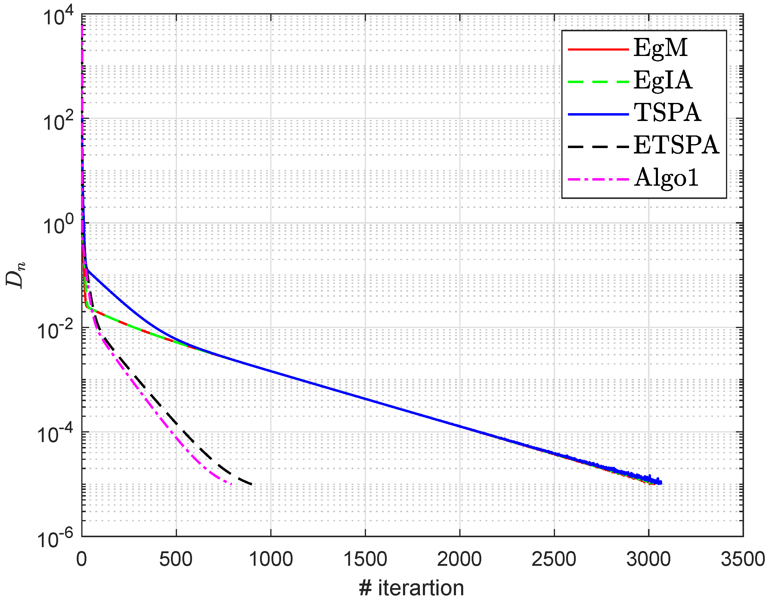
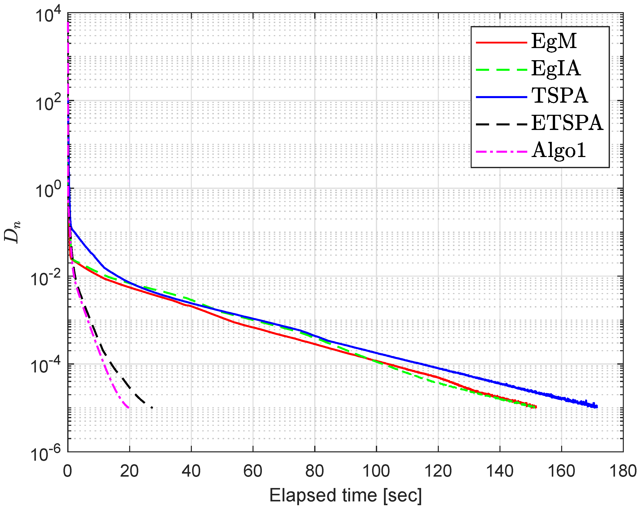
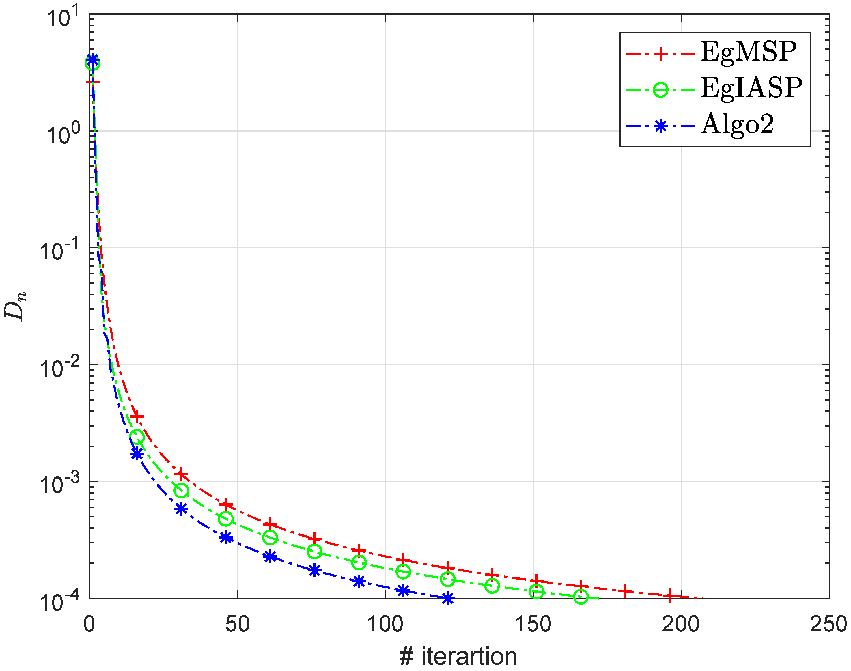
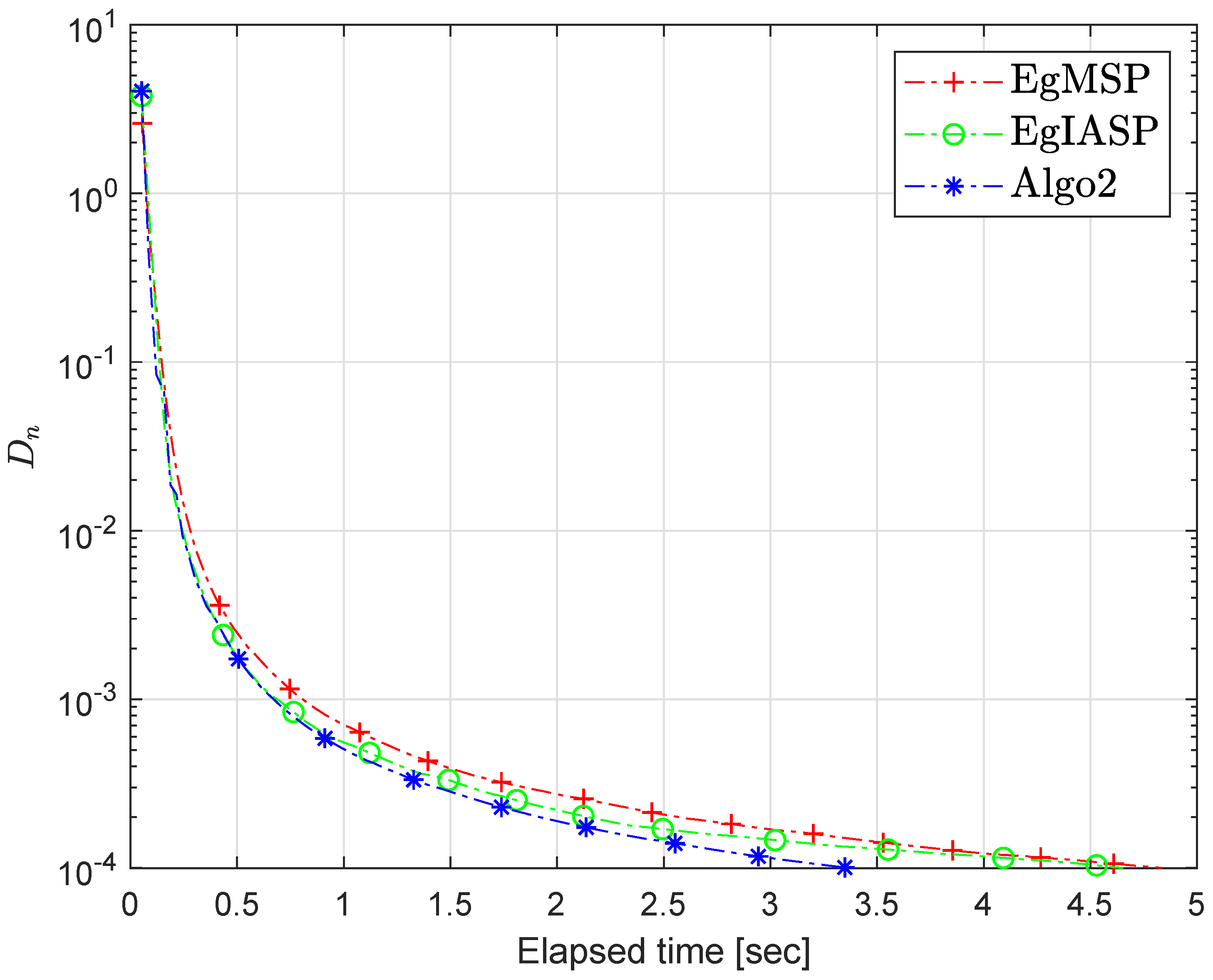
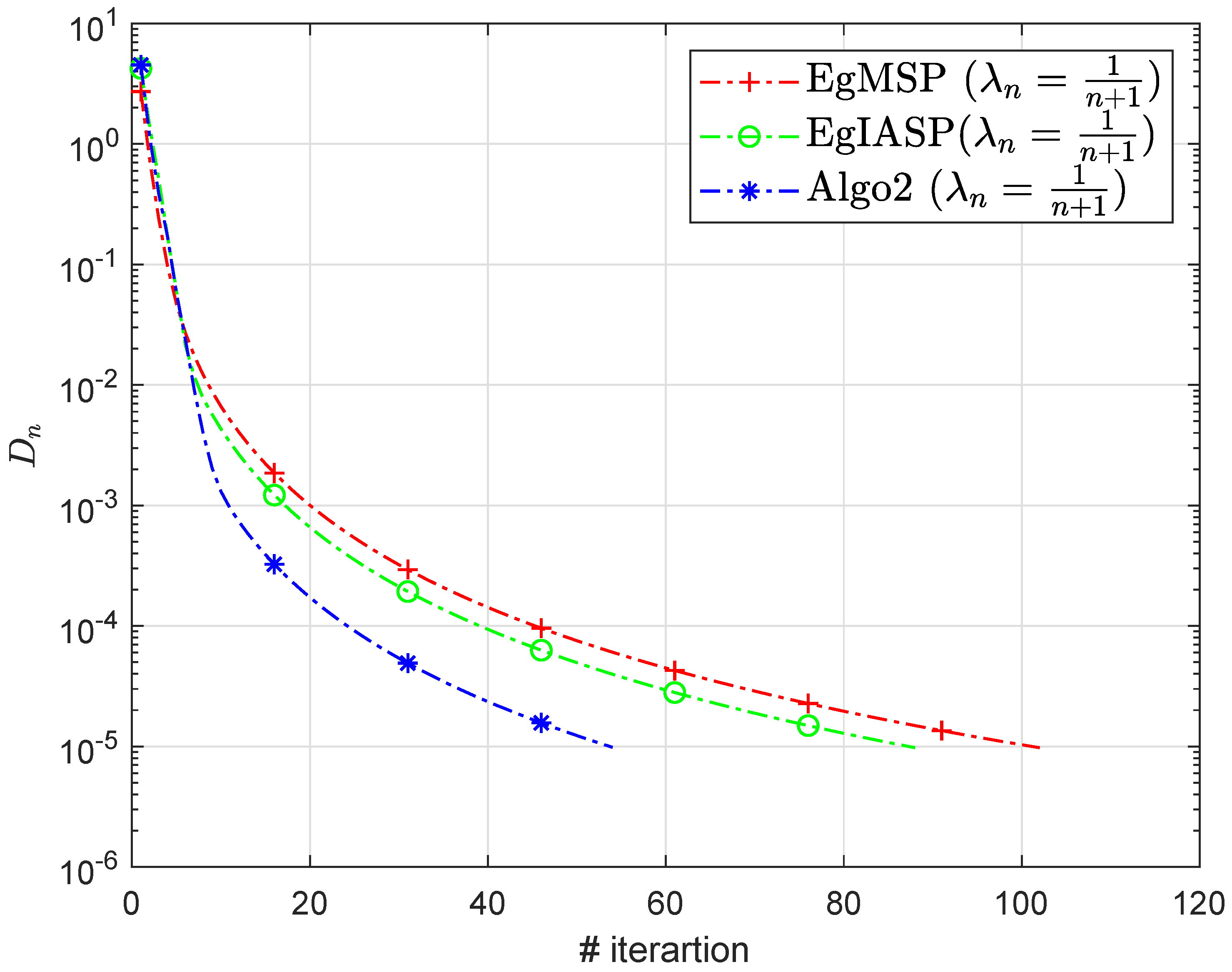
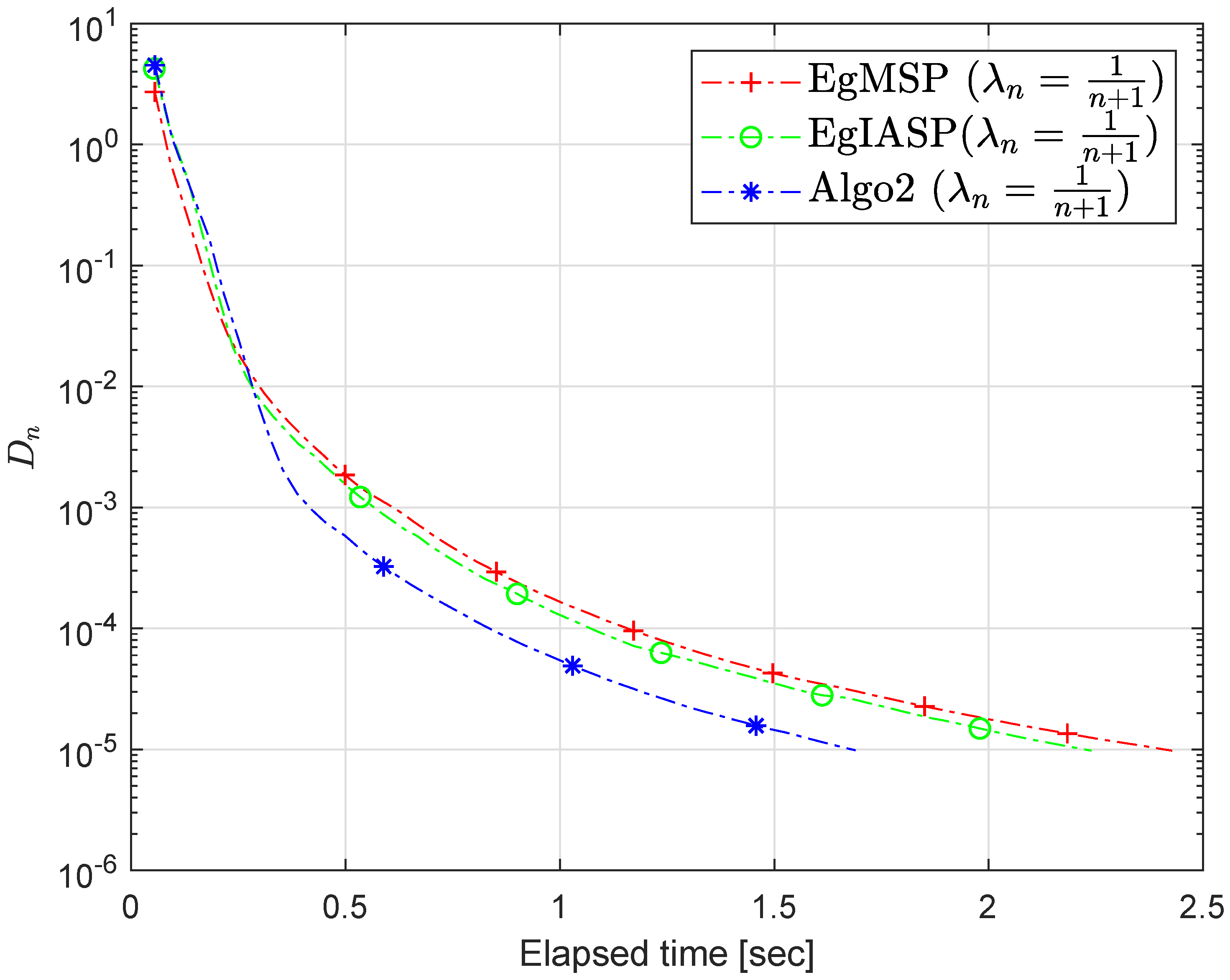
This paper is arranged as follows: Section 2 includes a number of definitions and basic results. Section 3 and Section 4 contain both of our methods involving the pseudomonotone and strongly pseudomonotone bifunction, as well as the convergence theorem. Section 5 covers the applications of our proposed results to the variational inequality problems. Section 6 illustrates numerical experiments in comparison with other existing algorithms using the Nash–Cournot equilibrium models to display the efficiency of our proposed algorithms.

2. Preliminaries

We make use of K as a closed, convex subset of the Hilbert space $\mathbb{E}.$ We denote $u_n\to p^{*}$ and $u_n\rightharpoonup p^{*}$ as the sequence $\left\{u_n\right\}$ strongly converges to $p^{*}$ and $\left\{u_n\right\}$ weakly converges to $p^{*}$, respectively. In addition, $EP(f,K)$ indicates the set of solutions of the equilibrium problem within K and $p^{*}\in EP(f,K).$

Definition 1.

Let a convex function $g:K\to \mathbb{R}$, and a subdifferential of g at $u\in K$ is:

$$\partial g\left(u\right)=\{w\in \mathbb{E}:g(v)-g(u)\ge \langle w,v-u\rangle ,\mathrm{for}\mathit{all}v\in K\}.$$

Definition 2.

The normal cone of K at $u\in K$ is:

$$N_K\left(u\right)=\{w\in \mathbb{E}:\langle w,v-u\rangle \le 0,\mathrm{for}\mathit{all}v\in K\}.$$

Definition 3.

The metric projection $P_K\left(u\right)$ of u onto a closed, convex subset K of $\mathbb{E}$ is defined as:

$$P_K\left(u\right)=\underset{}{argmin}\{\parallel v-u\parallel :v\in K\}.$$

Now, we consider the concepts of the monotonicity of a bifunction (see [1,43]).

Definition 4.

Let a bifunction $f:\mathbb{E}\times \mathbb{E}\to \mathbb{R}$ on K for $\gamma >0$ be said to be:

(1)

strongly monotone if:

$$f(u,v)+f(v,u)\le {-\gamma \parallel u-v\parallel }^2,\forall u,v\in K;$$

(2)

monotone if:

$$f(u,v)+f(v,u)\le 0,\forall u,v\in K;$$

(3)

strongly pseudomonotone if:

$$f(u,v)\ge 0⟹f(v,u)\le {-\gamma \parallel u-v\parallel }^2,\forall u,v\in K;$$

(4)

pseudomonotone if:

$$f(u,v)\ge 0⟹f(v,u)\le 0,\forall u,v\in K;$$

(5)

satisfying the Lipschitz-type condition on K if there exist two numbers $k_1,k_2>0,$ such that:

$$f(u,z)\le f(u,v)+f(v,z)+k_1{\parallel u-v\parallel }^2+k_2{\parallel v-z\parallel }^2,\forall u,v,z\in K.$$

Lemma 1

([44]).Let K be a nonempty, closed, and convex subset of a Hilbert space $\mathbb{E}$ and $g:K\to \mathbb{R}$ be a convex, subdifferentiable, and lower semi-continuous function. An element $u\in K$ is a minimizer of a function g if and only if $0\in \partial g\left(u\right)+N_K\left(u\right)$ where $\partial g\left(u\right)$ and $N_K\left(u\right)$ denote the subdifferential of g at u and the normal cone of K at u, respectively.

Lemma 2

([45]).Let $a,b\in \mathbb{E}$ and $\mu \in \mathbb{R}$, then the following is true:

$${\parallel \mu a+(1-\mu )b\parallel }^2={\mu \parallel a\parallel }^2+{(1-\mu )\parallel b\parallel }^2-\mu (1-\mu ){\parallel a-b\parallel }^2.$$

Lemma 3

([46]).Let $a_n$, $b_n$, and $c_n$ be a sequence in $[0,+\infty )$ such that:

$$a_{n+1}\le a_n+b_n(a_n-a_{n-1})+c_n,\forall n\ge 1,\mathrm{with}\sum _{n=1}^{+\infty }{c}_n<+\infty ,$$

and also, there exists $b>0$ such that $0\le b_n\le b<1,$ $\forall n\in \mathbb{N}.$ Then, we have:

(i)

${\displaystyle \sum _{n=1}^{+\infty }{[a_n-a_{n-1}]}_{+}<\infty ,}$ with ${\left[s\right]}_{+}:=max\{s,0\};$

(ii)

${lim}_{n\to +\infty }{a}_n=a^{*}\in [0,\infty ).$

Lemma 4

([47]).Let $\left\{{\xi }_n\right\}$ belong in $\mathbb{E}$ and $K\subset \mathbb{E}$ satisfying:

(i)

For $\xi \in K,$ ${lim}_{n\to \infty }\parallel {\xi }_n-\xi \parallel$ exists;

(ii)

Every weak cluster point of the sequence $\left\{{\xi }_n\right\}$ belongs to K.

Then, $\left\{{\xi }_n\right\}$ converges weakly to an element of $K.$

Lemma 5

([48]).Let $\left\{p_n\right\},\left\{q_n\right\}\subset [0,\infty )$ be sequences and ${\displaystyle \sum _{n=1}^{+\infty }{p}_n=\infty }$ with ${\displaystyle \sum _{n=1}^{+\infty }{p}_n{q}_n<\infty ,}$ then ${lim\; inf}_{n\to \infty }{q}_n=0.$

3. An Algorithm for the Pseudomonotone Equilibrium Problem and Its Convergence Analysis

The first method is developed by adding an inertial term to Algorithm 1 ([34], p. 4). It is important to note that the algorithm in the paper [34] cannot be used practically without knowledge of the Lipschitz-type constants of the bifunction. To overcome this situation, we suggest a new step-size rule that does not depend on Lipschitz-type constants. Rather, it depends on certain previous iterations and updates on each iteration. In a situation where Lipschitz constants are unknown or difficult to calculate, this approach is very useful. The following is our first algorithm in more detail:

Algorithm 1 Two-step proximal iterative method for pseudomonotone EP.

Initialization: Choose $u_{-1},v_{-1}\in K,$ ${\lambda }_0>0$ and $\mu \in [0,g(\alpha \left)\right).$ Set: $$u_0=\underset{y\in K}{argmin}\{{\lambda }_{0}f(v_{-1},y)+\frac{1}{2}\parallel u_{-1}{-y\parallel }^2\}\mathrm{and}{v}_0=\underset{y\in K}{argmin}\{{\lambda }_{0}f(v_{-1},y)+\frac{1}{2}\parallel u_0-y{\parallel }^2\}.$$ Iterative steps: Now, $v_{n-1},$ $v_n,$ $u_{n-1},$ $u_n\in K$ and ${\lambda }_n$ are known for $n\ge 0$. Step 1: Construct a half space: $${\Pi }_n=\{z\in \mathbb{E}:\langle u_n-{\lambda }_n{\omega }_n-v_n,z-v_n\rangle \le 0\}$$ where ${\omega }_n\in \partial f(v_{n-1},v_n)$, and then, compute: $$u_{n+1}={\mathrm{Prox}}_{{\lambda }_{n}f(v_n,.)}{t}_n=\underset{y\in {\Pi }_n}{argmin}\{{\lambda }_{n}f(v_n,y)+\frac{1}{2}\parallel t_n-y{\parallel }^2\},$$ where $t_n=u_n+{\alpha }_n(u_n-u_{n-1})$ and ${\alpha }_n\subset [0,\frac{1}{6})$ is a nondecreasing sequence. Step 2: Set $d=f(v_{n-1},u_{n+1})-f(v_{n-1},v_n)-f(v_n,u_{n+1})$ with: $${\lambda }_{n+1}=\left\{\begin{array}{cc}min\left\{{\lambda }_n,\frac{\mu (\parallel v_{n-1}-v_n{\parallel }^2+\parallel u_{n+1}-v_n{\parallel }^2)}{2d}\right\}\mathrm{if}\hfill & \hfill d>0;\\ {\lambda }_n\hfill & \hfill \mathrm{otherwise}.\end{array}\right.$$ Compute: $$v_{n+1}={\mathrm{Prox}}_{{\lambda }_{n+1}f(v_n,.)}{u}_{n+1}=\underset{y\in K}{argmin}\{{\lambda }_{n+1}f(v_n,y)+\frac{1}{2}\parallel u_{n+1}-y{\parallel }^2\}.$$ Step 3: If $u_{n+1}=v_n=t_n$, STOP; otherwise, set $n:=n+1$, and return back to Step 1.

Assumption 1.

Let a bifunction $f:\mathbb{E}\times \mathbb{E}\to \mathbb{R}$ satisfy the following conditions:

(A1)

f is pseudomonotone on K with $f(u,u)=0,$ for all $u\in K$;

(A2)

f satisfies the Lipschitz-type condition on $\mathbb{E}$ with $k_1$ and $k_2$;

(A3)

${lim}_{n\to \infty }supf(u_n,y)\le f(p,y)$ for each $y\in K$ and $\left\{u_n\right\}\subset K$ with $u_n\rightharpoonup p$;

(A4)

$f(u,.)$ is subdifferentiable and convex on $\mathbb{E}$ for each $u\in \mathbb{E}.$

Lemma 6.

We have the following inequality from Algorithm 1.

$${\lambda }_{n}f(v_n,y)-{\lambda }_{n}f(v_n,u_{n+1})\ge \langle t_n-u_{n+1},y-u_{n+1}\rangle ,\forall y\in {\Pi }_n.$$

Proof. 

By the value of $u_{n+1}$ with Lemma 1, we have:

$$0\in {\partial }_2\left\{{\lambda }_{n}f(v_n,y)+\frac{1}{2}{\parallel t_n-y\parallel }^2\right\}\left(u_{n+1}\right)+N_{{\Pi }_n}\left(u_{n+1}\right).$$

Thus, for $\omega \in {\partial }_{2}f(v_n,u_{n+1})$, there exists $\overline{\omega }\in N_{{\Pi }_n(}{u}_{n+1})$ such that:

$${\lambda }_n\omega +u_{n+1}-t_n+\overline{\omega }=0,$$

which gives:

$$\langle t_n-u_{n+1},y-u_{n+1}\rangle ={\lambda }_n\langle \omega ,y-u_{n+1}\rangle +\langle \overline{\omega },y-u_{n+1}\rangle ,\forall y\in {\Pi }_n.$$

By $\overline{\omega }\in N_{{\Pi }_n}\left(u_{n+1}\right)$, we have $\langle \overline{\omega },y-u_{n+1}\rangle \le 0,$ $\forall y\in {\Pi }_n.$ This implies that:

$$\langle t_n-u_{n+1},y-u_{n+1}\rangle \le {\lambda }_n\langle \omega ,y-u_{n+1}\rangle ,\forall y\in {\Pi }_n.$$

(4)

From $\omega \in \partial f(v_n,u_{n+1})$ and by the subdifferential definition, we have:

$$f(v_n,y)-f(v_n,u_{n+1})\ge \langle \omega ,y-u_{n+1}\rangle ,\forall y\in \mathbb{E}.$$

(5)

Combining (4) and (5), we obtain:

$${\lambda }_{n}f(v_n,y)-{\lambda }_{n}f(v_n,u_{n+1})\ge \langle t_n-u_{n+1},y-u_{n+1}\rangle ,\forall y\in {\Pi }_n.$$

□

Lemma 7.

We also have the following expression from Algorithm 1.

$${\lambda }_{n+1}f(v_n,y)-{\lambda }_{n+1}f(v_n,v_{n+1})\ge \langle u_{n+1}-v_{n+1},y-v_{n+1}\rangle ,\forall y\in K.$$

Proof. 

The proof is identical to the proof of Lemma 6. □

Remark 1.

By taking $u_{n+1}=v_n=t_n$ and $u_{n+1}=v_n=v_{n+1}$ in Algorithm 1, we can get $v_n\in EP(f,K)$ from Lemma 6 and Lemma 7, respectively.

Lemma 8.

We have the following relationship from Algorithm 1.

$${\lambda }_n\left\{f(v_{n-1},u_{n+1})-f(v_{n-1},v_n)\right\}\ge \langle u_n-v_n,u_{n+1}-v_n\rangle .$$

Proof. 

Since $u_{n+1}\in {\Pi }_n,$ this gives that $\langle u_n-{\lambda }_n{\omega }_n-v_n,u_{n+1}-v_n\rangle \le 0.$ Thus, we get:

$${\lambda }_n\langle {\omega }_n,u_{n+1}-v_n\rangle \ge \langle u_n-v_n,u_{n+1}-v_n\rangle .$$

(6)

By ${\omega }_n\in \partial f(v_{n-1},v_n)$ and the definition of subdifferential, we get:

$$f(v_{n-1},y)-f(v_{n-1},v_n)\ge \langle {\omega }_n,y-v_n\rangle ,\forall y\in \mathbb{E}.$$

Substituting $y=u_{n+1}$ in the above inequality, we get:

$$f(v_{n-1},u_{n+1})-f(v_{n-1},v_n)\ge \langle {\omega }_n,u_{n+1}-v_n\rangle ,\forall y\in \mathbb{E}.$$

(7)

Combining (6) and (7), we have:

$${\lambda }_n\left\{f(v_{n-1},u_{n+1})-f(v_{n-1},v_n)\right\}\ge \langle u_n-v_n,u_{n+1}-v_n\rangle .$$

□

Lemma 9.

Let $f:\mathbb{E}\times \mathbb{E}\to \mathbb{R}$ satisfy Assumption 1. Then, for each $p^{*}\in EP(f,K)\ne \varnothing ,$ we have:

$$\begin{array}{cc}\hfill \parallel u_{n+1}-p^{*}{\parallel }^2& \le \parallel t_n-p^{*}{\parallel }^2-\left(1-\frac{2\mu {\lambda }_n}{{\lambda }_{n+1}}\right)\parallel u_n-v_n{\parallel }^2-\left(1-\frac{\mu {\lambda }_n}{{\lambda }_{n+1}}\right){\parallel u_{n+1}-v_n\parallel }^2\hfill \\ \hfill & +\frac{2\mu {\lambda }_n}{{\lambda }_{n+1}}\parallel u_n-v_{n-1}{\parallel }^2-\parallel u_{n+1}-t_n{\parallel }^2+{\parallel u_n-u_{n+1}\parallel }^2.\hfill \end{array}$$

Proof. 

It follows from Lemma 6 with $y=p^{*}$ that we have:

$${\lambda }_{n}f(v_n,p^{*})-{\lambda }_{n}f(v_n,u_{n+1})\ge \langle t_n-u_{n+1},p^{*}-u_{n+1}\rangle .$$

(8)

Thus, $f(p^{*},v_n)\ge 0$, and due to Condition (A1), we have $f(v_n,p^{*})\le 0.$ This implies that:

$$\langle t_n-u_{n+1},u_{n+1}-p^{*}\rangle \ge {\lambda }_{n}f(v_n,u_{n+1}).$$

(9)

By the definition, ${\lambda }_{n+1}$ implies that:

$$f(v_{n-1},u_{n+1})-f(v_{n-1},v_n)-f(v_n,u_{n+1})\le \frac{\mu (\parallel v_{n-1}-v_n{\parallel }^2+\parallel u_{n+1}-v_n{\parallel }^2)}{2{\lambda }_{n+1}}$$

both sides have been multiplied with ${\lambda }_n>0,$ such that:

$$\begin{array}{c}\hfill {\lambda }_{n}f(v_n,u_{n+1})\ge {\lambda }_{n}f(v_{n-1},u_{n+1})-{\lambda }_{n}f(v_{n-1},v_n)-\frac{{\lambda }_n\mu (\parallel v_{n-1}-v_n{\parallel }^2+\parallel u_{n+1}-v_n{\parallel }^2)}{2{\lambda }_{n+1}}\end{array}$$

(10)

By combing (9) and (10), we have:

$$\begin{array}{c}\hfill \langle t_n-u_{n+1},u_{n+1}-p^{*}\rangle \ge {\lambda }_n\{f(v_{n-1},u_{n+1})-f(v_{n-1},v_n)\}-\frac{\mu {\lambda }_n}{2{\lambda }_{n+1}}\parallel v_{n-1}-v_n{\parallel }^2-\frac{\mu {\lambda }_n}{2{\lambda }_{n+1}}{\parallel u_{n+1}-v_n\parallel }^2.\end{array}$$

(11)

Since $u_{n+1}\in {\Pi }_n$, then from Lemma 8, we have:

$${\lambda }_n\left\{f(v_{n-1},u_{n+1})-f(v_{n-1},v_n)\right\}\ge \langle u_n-v_n,u_{n+1}-v_n\rangle .$$

(12)

From (11) and (12), we obtain:

$$\begin{array}{c}\hfill \langle t_n-u_{n+1},u_{n+1}-p^{*}\rangle \ge \langle u_n-v_n,u_{n+1}-v_n\rangle -\frac{\mu {\lambda }_n}{2{\lambda }_{n+1}}\parallel v_{n-1}-v_n{\parallel }^2-\frac{\mu {\lambda }_n}{2{\lambda }_{n+1}}{\parallel u_{n+1}-v_n\parallel }^2.\end{array}$$

(13)

We have the following facts:

$$2\langle t_n-u_{n+1},u_{n+1}-p^{*}\rangle =\parallel t_n-p^{*}{\parallel }^2-\parallel u_{n+1}-t_n{\parallel }^2-{\parallel u_{n+1}-p^{*}\parallel }^2,$$

$$2\langle v_n-u_n,v_n-u_{n+1}\rangle =\parallel u_n-v_n{\parallel }^2+\parallel u_{n+1}-v_n{\parallel }^2-{\parallel u_n-u_{n+1}\parallel }^2,$$

and:

$$\parallel v_{n-1}-v_n{\parallel }^2\le {\left(\parallel v_{n-1}-u_n\parallel +\parallel u_n-v_n\parallel \right)}^2\le 2\parallel v_{n-1}-u_n{\parallel }^2+2{\parallel u_n-v_n\parallel }^2.$$

From above facts with Expression (13) complete the proof. □

Theorem 1.

The sequences $\left\{t_n\right\},$ $\left\{v_n\right\}$, and $\left\{u_n\right\}$ are generated by Algorithm 1 and weakly converge to $p^{*},$ where:

$$0<\mu <\frac{1-6\alpha }{3}\mathrm{and}0\le {\alpha }_n\le \alpha <\frac{1}{6}.$$

Proof. 

Adding to both sides the value $\frac{2\mu {\lambda }_{n+1}}{{\lambda }_{n+2}}{\parallel u_{n+1}-v_n\parallel }^2$ in Lemma 9, we have:

$$\begin{array}{cc}\hfill & \parallel u_{n+1}-p^{*}{\parallel }^2+\frac{2\mu {\lambda }_{n+1}}{{\lambda }_{n+2}}{\parallel u_{n+1}-v_n\parallel }^2\hfill \\ \hfill & \le \parallel t_n-p^{*}{\parallel }^2-\left(1-\frac{2\mu {\lambda }_n}{{\lambda }_{n+1}}\right)\parallel u_n-v_n{\parallel }^2-\left(1-\frac{\mu {\lambda }_n}{{\lambda }_{n+1}}\right){\parallel u_{n+1}-v_n\parallel }^2\hfill \\ \hfill & +\frac{2\mu {\lambda }_n}{{\lambda }_{n+1}}\parallel u_n-v_{n-1}{\parallel }^2-\parallel u_{n+1}-t_n{\parallel }^2+\parallel u_{n+1}-u_n{\parallel }^2+\frac{2\mu {\lambda }_{n+1}}{{\lambda }_{n+2}}{\parallel u_{n+1}-v_n\parallel }^2\hfill \end{array}$$

(14)

$$\begin{array}{cc}\hfill & \le \parallel t_n-p^{*}{\parallel }^2-\left(1-\frac{2\mu {\lambda }_n}{{\lambda }_{n+1}}\right)\parallel u_n-v_n{\parallel }^2-\left(1-\frac{\mu {\lambda }_n}{{\lambda }_{n+1}}-\frac{2\mu {\lambda }_n}{{\lambda }_{n+2}}\right){\parallel u_{n+1}-v_n\parallel }^2\hfill \\ \hfill & +\frac{2\mu {\lambda }_n}{{\lambda }_{n+1}}\parallel u_n-v_{n-1}{\parallel }^2-\parallel u_{n+1}-t_n{\parallel }^2+{\parallel u_{n+1}-u_n\parallel }^2\hfill \end{array}$$

(15)

$$\begin{array}{cc}\hfill & \le \parallel t_n-p^{*}{\parallel }^2-\left(1-\frac{\mu {\lambda }_n}{{\lambda }_{n+1}}-\frac{2\mu {\lambda }_n}{{\lambda }_{n+2}}\right)\left[\parallel u_{n+1}-v_n{\parallel }^2+{\parallel u_n-v_n\parallel }^2\right]\hfill \\ \hfill & +\frac{2\mu {\lambda }_n}{{\lambda }_{n+1}}\parallel u_n-v_{n-1}{\parallel }^2-\parallel u_{n+1}-t_n{\parallel }^2+{\parallel u_{n+1}-u_n\parallel }^2\hfill \end{array}$$

(16)

$$\begin{array}{cc}\hfill & \le \parallel t_n-p^{*}{\parallel }^2-\frac{1}{2}\left(1-\frac{\mu {\lambda }_n}{{\lambda }_{n+1}}-\frac{2\mu {\lambda }_n}{{\lambda }_{n+2}}\right){\left[\parallel u_{n+1}-v_n\parallel +\parallel u_n-v_n\parallel \right]}^2\hfill \\ \hfill & +\frac{2\mu {\lambda }_n}{{\lambda }_{n+1}}\parallel u_n-v_{n-1}{\parallel }^2-\parallel u_{n+1}-t_n{\parallel }^2+{\parallel u_{n+1}-u_n\parallel }^2\hfill \end{array}$$

(17)

$$\begin{array}{cc}\hfill & \le \parallel t_n-p^{*}{\parallel }^2-\frac{1}{2}\left(1-\frac{\mu {\lambda }_n}{{\lambda }_{n+1}}-\frac{2\mu {\lambda }_n}{{\lambda }_{n+2}}\right){\parallel u_{n+1}-u_n\parallel }^2\hfill \\ \hfill & +\frac{2\mu {\lambda }_n}{{\lambda }_{n+1}}\parallel u_n-v_{n-1}{\parallel }^2-\parallel u_{n+1}-t_n{\parallel }^2+{\parallel u_{n+1}-u_n\parallel }^2.\hfill \end{array}$$

(18)

By the definition of $t_n$ in Algorithm 1, we get:

$$\begin{array}{cc}\hfill \parallel t_n-p^{*}{\parallel }^2& =\parallel u_n+{\alpha }_n(u_n-u_{n-1})-p^{*}{\parallel }^2\hfill \\ \hfill & =\parallel (1+{\alpha }_n)(u_n-p^{*})-{\alpha }_n(u_{n-1}-p^{*}){\parallel }^2\hfill \\ \hfill & =(1+{\alpha }_n)\parallel u_n-p^{*}{\parallel }^2-{\alpha }_n\parallel u_{n-1}-p^{*}{\parallel }^2+{\alpha }_n(1+{\alpha }_n){\parallel u_n-u_{n-1}\parallel }^2.\hfill \end{array}$$

(19)

The value of $u_{n+1}$ with Lemma 2 gives:

$$\begin{array}{cc}\hfill \parallel u_{n+1}-t_n{\parallel }^2& =\parallel u_{n+1}-u_n-{\alpha }_n(u_n-u_{n-1}){\parallel }^2\hfill \\ \hfill & =\parallel u_{n+1}-u_n{\parallel }^2+{\alpha }_n^2{\parallel u_n-u_{n-1}\parallel }^2-2{\alpha }_n\langle u_{n+1}-u_n,u_n-u_{n-1}\rangle \hfill \\ \hfill & \ge \parallel u_{n+1}-u_n{\parallel }^2+{\alpha }_n^2\parallel u_n-u_{n-1}{\parallel }^2-2{\alpha }_n\parallel u_{n+1}-u_n\parallel \parallel u_n-u_{n-1}\parallel \hfill \end{array}$$

(20)

$$\begin{array}{cc}\hfill & \ge \parallel u_{n+1}-u_n{\parallel }^2+{\alpha }_n^2\parallel u_n-u_{n-1}{\parallel }^2-{\alpha }_n\parallel u_{n+1}-u_n{\parallel }^2-{\alpha }_n{\parallel u_n-u_{n-1}\parallel }^2\hfill \\ \hfill & \ge (1-{\alpha }_n)\parallel u_{n+1}-u_n{\parallel }^2+({\alpha }_n^2-{\alpha }_n){\parallel u_n-u_{n-1}\parallel }^2.\hfill \end{array}$$

(21)

Thus, Expression (18) with (19) and (21) turns into:

$$\begin{array}{cc}\hfill & \parallel u_{n+1}-p^{*}{\parallel }^2+\frac{2\mu {\lambda }_{n+1}}{{\lambda }_{n+2}}{\parallel u_{n+1}-v_n\parallel }^2\hfill \\ \hfill & \le (1+{\alpha }_n)\parallel u_n-p^{*}{\parallel }^2-{\alpha }_n\parallel u_{n-1}-p^{*}{\parallel }^2+{\alpha }_n(1+{\alpha }_n){\parallel u_n-u_{n-1}\parallel }^2\hfill \\ \hfill & -\frac{1}{2}\left(1-\frac{\mu {\lambda }_n}{{\lambda }_{n+1}}-\frac{2\mu {\lambda }_n}{{\lambda }_{n+2}}\right)\parallel u_{n+1}-u_n{\parallel }^2+\frac{2\mu {\lambda }_n}{{\lambda }_{n+1}}{\parallel u_n-v_{n-1}\parallel }^2\hfill \\ \hfill & +\parallel u_{n+1}-u_n{\parallel }^2-(1-{\alpha }_n)\parallel u_{n+1}-u_n{\parallel }^2-({\alpha }_n^2-{\alpha }_n){\parallel u_n-u_{n-1}\parallel }^2\hfill \end{array}$$

(22)

$$\begin{array}{cc}\hfill & \le (1+{\alpha }_n)\parallel u_n-p^{*}{\parallel }^2-{\alpha }_n\parallel u_{n-1}-p^{*}{\parallel }^2+\frac{2\mu {\lambda }_n}{{\lambda }_{n+1}}{\parallel u_n-v_{n-1}\parallel }^2\hfill \\ \hfill & -\left(\frac{1}{2}-\frac{\mu {\lambda }_n}{2{\lambda }_{n+1}}-\frac{\mu {\lambda }_n}{{\lambda }_{n+2}}-{\alpha }_n\right)\parallel u_{n+1}-u_n{\parallel }^2+2{\alpha }_n{\parallel u_n-u_{n-1}\parallel }^2\hfill \end{array}$$

(23)

$$\begin{array}{cc}\hfill & \le (1+{\alpha }_n)\parallel u_n-p^{*}{\parallel }^2-{\alpha }_n\parallel u_{n-1}-p^{*}{\parallel }^2+\frac{2\mu {\lambda }_n}{{\lambda }_{n+1}}{\parallel u_n-v_{n-1}\parallel }^2\hfill \\ \hfill & -{\kappa }_n\parallel u_{n+1}-u_n{\parallel }^2+{\xi }_n{\parallel u_n-u_{n-1}\parallel }^2,\hfill \end{array}$$

(24)

where ${\kappa }_n:=\left(\frac{1}{2}-\frac{\mu {\lambda }_n}{2{\lambda }_{n+1}}-\frac{\mu {\lambda }_n}{{\lambda }_{n+2}}-{\alpha }_n\right)\mathrm{and}{\xi }_n:=2{\alpha }_n.$ By Substituting:

$${\Gamma }_n=\parallel u_n-p^{*}{\parallel }^2-{\alpha }_n\parallel u_{n-1}-p^{*}{\parallel }^2+\frac{2\mu {\lambda }_n}{{\lambda }_{n+1}}\parallel u_n-v_{n-1}{\parallel }^2+{\xi }_n{\parallel u_n-u_{n-1}\parallel }^2.$$

Next, we compute:

$$\begin{array}{cc}\hfill {\Gamma }_{n+1}-{\Gamma }_n& =\parallel u_{n+1}-p^{*}{\parallel }^2-{\alpha }_{n+1}\parallel u_n-p^{*}{\parallel }^2+\frac{2\mu {\lambda }_{n+1}}{{\lambda }_{n+2}}\parallel u_{n+1}-v_n{\parallel }^2+{\xi }_{n+1}{\parallel u_{n+1}-u_n\parallel }^2\hfill \\ \hfill & -\parallel u_n-p^{*}{\parallel }^2+{\alpha }_n\parallel u_{n-1}-p^{*}{\parallel }^2-\frac{2\mu {\lambda }_n}{{\lambda }_{n+1}}\parallel u_n-v_{n-1}{\parallel }^2-{\xi }_n{\parallel u_n-u_{n-1}\parallel }^2\hfill \\ \hfill & \le \parallel u_{n+1}-p^{*}{\parallel }^2-(1+{\alpha }_n)\parallel u_n-p^{*}{\parallel }^2+{\alpha }_n\parallel u_{n-1}-p^{*}{\parallel }^2+\frac{2\mu {\lambda }_{n+1}}{{\lambda }_{n+2}}{\parallel u_{n+1}-v_n\parallel }^2\hfill \\ \hfill & +{\xi }_{n+1}\parallel u_{n+1}-u_n{\parallel }^2-{\xi }_n\parallel u_n-u_{n-1}{\parallel }^2-\frac{2\mu {\lambda }_n}{{\lambda }_{n+1}}{\parallel u_n-v_{n-1}\parallel }^2.\hfill \end{array}$$

(25)

From Expression (24) with (25), we obtain:

$$\begin{array}{c}{\Gamma }_{n+1}-{\Gamma }_n\le -{\kappa }_n\parallel u_{n+1}-u_n{\parallel }^2+{\xi }_{n+1}\parallel u_{n+1}-u_n{\parallel }^2=-({\kappa }_n-{\xi }_{n+1}){\parallel u_{n+1}-u_n\parallel }^2,\end{array}$$

(26)

and we continue to evaluate:

$$\begin{array}{cc}\hfill {\kappa }_n-{\xi }_{n+1}& =\frac{1}{2}-\frac{\mu {\lambda }_n}{2{\lambda }_{n+1}}-\frac{\mu {\lambda }_n}{{\lambda }_{n+2}}-{\alpha }_n-2{\alpha }_{n+1}\ge \left(\frac{1}{2}-3\alpha \right)-\mu \left(\frac{{\lambda }_n}{2{\lambda }_{n+1}}+\frac{{\lambda }_n}{{\lambda }_{n+2}}\right).\hfill \end{array}$$

(27)

Due to ${\lambda }_n\to \lambda ,$ the above implies that:

$$\left(\frac{1}{2}-3\alpha \right)-\mu \left(\frac{{\lambda }_n}{2{\lambda }_{n+1}}+\frac{{\lambda }_n}{{\lambda }_{n+2}}\right)⟶\frac{1}{2}-3\alpha -\frac{3}{2}\mu >0\mathrm{as}n\to \infty .$$

Due to our supposition and from the above, there exists an $\delta \ge 0$ and $n_0\in \mathbb{N}$ such that:

$${\kappa }_n-{\xi }_{n+1}\ge \delta \ge 0,\forall n\ge n_0.$$

(28)

Thus, Expression (26) with (28) implies that:

$${\Gamma }_{n+1}-{\Gamma }_n\le -\delta {\parallel u_{n+1}-u_n\parallel }^2\le 0.$$

(29)

The sequence $\left\{{\Gamma }_n\right\}$ is non-increasing for $n\ge n_0$. By the value of ${\Gamma }_{n+1}$, we have:

$$\begin{array}{cc}\hfill {\Gamma }_{n+1}& =\parallel u_{n+1}-p^{*}{\parallel }^2-{\alpha }_{n+1}\parallel u_n-p^{*}{\parallel }^2+\frac{2\mu {\lambda }_{n+1}}{{\lambda }_{n+2}}\parallel u_{n+1}-v_n{\parallel }^2+{\xi }_{n+1}{\parallel u_{n+1}-u_n\parallel }^2\hfill \\ \hfill & \ge -{\alpha }_{n+1}{\parallel u_n-p^{*}\parallel }^2.\hfill \end{array}$$

(30)

From the value ${\Gamma }_n,$ we have:

$$\begin{array}{cc}\hfill {\Gamma }_n& =\parallel u_n-p^{*}{\parallel }^2-{\alpha }_n\parallel u_{n-1}-p^{*}{\parallel }^2+\frac{2\mu {\lambda }_n}{{\lambda }_{n+1}}\parallel u_n-v_{n-1}{\parallel }^2+{\xi }_n{\parallel u_n-u_{n-1}\parallel }^2\hfill \\ \hfill & \ge \parallel u_n-p^{*}{\parallel }^2-{\alpha }_n{\parallel u_{n-1}-p^{*}\parallel }^2.\hfill \end{array}$$

(31)

The expression (31) for $n\ge n_0$ implies that:

$$\begin{array}{cc}\hfill \parallel u_n-p^{*}{\parallel }^2& \le {\Gamma }_n+{\alpha }_n{\parallel u_{n-1}-p^{*}\parallel }^2\hfill \\ \hfill & \le {\Gamma }_{n_0}+\alpha {\parallel u_{n-1}-p^{*}\parallel }^2\hfill \\ \hfill & \le \cdots \le {\Gamma }_{n_0}({\alpha }^{n-n_0}+\cdots +1)+{\alpha }^{n-n_0}{\parallel u_{n_0}-p^{*}\parallel }^2\hfill \\ \hfill & \le \frac{{\Gamma }_{n_0}}{1-\alpha }+{\alpha }^{n-n_0}{\parallel u_{n_0}-p^{*}\parallel }^2.\hfill \end{array}$$

(32)

It follows from Expressions (30) and (32) that:

$$\begin{array}{c}\hfill -{\Gamma }_{n+1}\le {\alpha }_{n+1}\parallel u_n-p^{*}{\parallel }^2\le \alpha \parallel u_n-p^{*}{\parallel }^2\le \alpha \frac{{\Gamma }_{n_0}}{1-\alpha }+{\alpha }^{n-n_0+1}{\parallel u_{n_0}-p^{*}\parallel }^2.\end{array}$$

(33)

It follows from Expressions (29) and (33) that:

$$\begin{array}{cc}\hfill \delta \sum _{n=n_0}^k{\parallel u_{n+1}-u_n\parallel }^2& \le {\Gamma }_{n_0}-{\Gamma }_{n+1}\hfill \\ \hfill & \le {\Gamma }_{n_0}+\alpha \frac{{\Gamma }_{n_0}}{1-\alpha }+{\alpha }^{n-n_0+1}{\parallel u_{n_0}-p^{*}\parallel }^2\hfill \\ \hfill & \le \frac{{\Gamma }_{n_0}}{1-\alpha }+{\parallel u_{n_0}-p^{*}\parallel }^2,\hfill \end{array}$$

(34)

and letting $k\to \infty$ in Expression (34), we obtain:

$$\sum _{n=1}^{\infty }\parallel u_{n+1}-u_n{\parallel }^2<+\infty ,\mathrm{implies}\mathrm{that}\parallel u_{n+1}-u_n\parallel \to 0\mathrm{as}n\to \infty .$$

(35)

From Expressions (20) and (35), we have:

$$\underset{n\to \infty }{lim}\parallel u_{n+1}-t_n\parallel \to 0,$$

(36)

and also to continue:

$$0\le \parallel u_n-t_n\parallel \le \parallel u_n-u_{n+1}\parallel +\parallel u_{n+1}-t_n\parallel ⟶0\mathrm{as}n\to \infty .$$

(37)

Let ${\Delta }_n=\parallel u_n-p^{*}{\parallel }^2-{\alpha }_n\parallel u_{n-1}-p^{*}{\parallel }^2+\frac{2\mu {\lambda }_n}{{\lambda }_{n+1}}{\parallel u_n-v_{n-1}\parallel }^2.$ Expression (33) converts into:

$$-{\Delta }_{n+1}\le \alpha \frac{{\Gamma }_{n_0}}{1-\alpha }+{\alpha }^{n-n_0+1}\parallel u_{n_0}-p^{*}{\parallel }^2+{\xi }_{n+1}{\parallel u_n-u_{n-1}\parallel }^2.$$

(38)

By Expressions (16) and (19) with (38) for $n\ge n_0,$ we have:

$$\begin{array}{cc}\hfill & \left(1-\frac{\mu {\lambda }_n}{{\lambda }_{n+1}}-\frac{2\mu {\lambda }_n}{{\lambda }_{n+2}}\right)\left[\parallel u_n-v_n{\parallel }^2+{\parallel u_{n+1}-v_n\parallel }^2\right]\hfill \\ \hfill & \le {\Delta }_n-{\Delta }_{n+1}+{\alpha }_n(1+{\alpha }_n)\parallel u_n-u_{n-1}{\parallel }^2+{\parallel u_{n+1}-u_n\parallel }^2\hfill \\ \hfill & \le {\Delta }_n-{\Delta }_{n+1}+\alpha (1+\alpha )\parallel u_n-u_{n-1}{\parallel }^2+{\parallel u_{n+1}-u_n\parallel }^2.\hfill \end{array}$$

(39)

Due to the assumption on $\mu$ for some $ϵ>0,$

$$\left(1-\frac{\mu {\lambda }_n}{{\lambda }_{n+1}}-\frac{2\mu {\lambda }_n}{{\lambda }_{n+2}}\right)\ge ϵ>0,\mathrm{as}\ge n_0.$$

Let us fix $k\ge n_0$ and Expressions (38) and (39) for $n=n_0,n_0+1,\cdots ,k.$ Summing them, we have:

$$\begin{array}{cc}\hfill & ϵ\sum _{n=n_0}^k\parallel u_n-v_n{\parallel }^2+ϵ\sum _{n=n_0}^k{\parallel u_{n+1}-v_n\parallel }^2\hfill \\ \hfill & \le {\Delta }_{n_0}-{\Delta }_{k+1}+\alpha (1+\alpha )\sum _{n=n_0}^k\parallel u_n-u_{n-1}{\parallel }^2+\sum _{n=n_0}^k{\parallel u_{n+1}-u_n\parallel }^2\hfill \\ \hfill & \le {\Delta }_{n_0}+\alpha \frac{{\Delta }_{n_0}}{1-\alpha }+{\alpha }^{n-n_0+1}\parallel u_{n_0}-p^{*}{\parallel }^2+{\xi }_{k+1}{\parallel u_k-u_{k-1}\parallel }^2\hfill \\ \hfill & +\alpha (1+\alpha )\sum _{n=n_0}^k\parallel u_n-u_{n-1}{\parallel }^2+\sum _{n=n_0}^k{\parallel u_{n+1}-u_n\parallel }^2\hfill \end{array}$$

(40)

and letting $k\to \infty$ in the above expression leads to:

$$\sum _n\parallel u_n-v_n{\parallel }^2<\infty ,\sum _n{\parallel u_{n+1}-v_n\parallel }^2<\infty .$$

(41)

The above expression also implies that:

$$\underset{n\to \infty }{lim}\parallel u_n-v_n\parallel =\underset{n\to \infty }{lim}\parallel u_{n+1}-v_n\parallel =0.$$

(42)

By using the triangle inequality with Expression (42), we have:

$$0\le \parallel v_n-v_{n-1}\parallel \le \parallel u_n-v_n\parallel +\parallel u_n-v_{n-1}\parallel ⟶0,\mathrm{as}n\to \infty .$$

(43)

Next, from Expression (14) with (19):

$$\begin{array}{cc}\hfill \parallel u_{n+1}-p^{*}{\parallel }^2& \le (1+{\alpha }_n)\parallel u_n-p^{*}{\parallel }^2-{\alpha }_n\parallel u_{n-1}-p^{*}{\parallel }^2+\alpha (1+\alpha ){\parallel u_n-u_{n-1}\parallel }^2\hfill \\ \hfill & +\frac{2\mu {\lambda }_n}{{\lambda }_{n+1}}\parallel u_n-v_{n-1}{\parallel }^2+{\parallel u_{n+1}-u_n\parallel }^2\hfill \end{array}$$

(44)

and the above expression with (35), (41), and Lemma 3 implies that the limit of $\parallel u_n-p^{*}\parallel ,$ $\parallel t_n-p^{*}\parallel$ and $\parallel v_n-p^{*}\parallel$ exists for each $p^{*}\in EP(f,K),$ meaning that the sequences $\left\{u_n\right\}$, $\left\{t_n\right\}$, and $\left\{v_n\right\}$ are bounded. Next, we have to prove that each weak sequential limit point of the sequence $\left\{u_n\right\}$ belongs to $EP(f,K).$ Let z be any sequential weak cluster point of the sequence $\left\{u_n\right\},$ i.e., a weak convergent subsequence $\left\{u_{n_k}\right\}$ of $\left\{u_n\right\}$ converging to $z,$ which also implies that $\left\{v_{n_k}\right\}$ also converge weakly to $z.$ Now, our aim to show that $z\in EP(f,K).$ Using Lemma 6, the definition of ${\lambda }_{n+1}$ (10), and Lemma 8, we obtain:

$$\begin{array}{cc}\hfill {\lambda }_{n_k}f(v_{n_k},y)& \ge {\lambda }_{n_k}f(v_{n_k},u_{n_k+1})+\langle t_{n_k}-u_{n_k+1},y-u_{n_k+1}\rangle \hfill \\ \hfill & \ge {\lambda }_{n_k}f(v_{n_k-1},u_{n_{k+1}})-{\lambda }_{n_k}f(v_{n_k-1},v_{n_k})-\frac{\mu {\lambda }_{n_k}}{2{\lambda }_{n_k+1}}{\parallel v_{n_k}-v_{n_k-1}\parallel }^2\hfill \\ \hfill & -\frac{\mu {\lambda }_{n_k}}{2{\lambda }_{n_k+1}}{\parallel v_{n_k}-u_{n_k+1}\parallel }^2+\langle t_{n_k}-u_{n_k+1},y-u_{n_k+1}\rangle \hfill \\ \hfill & \ge \langle u_{n_k}-v_{n_k},u_{n_k+1}-v_{n_k}\rangle -\frac{\mu {\lambda }_{n_k}}{2{\lambda }_{n_k+1}}{\parallel v_{n_k}-v_{n_k-1}\parallel }^2\hfill \\ \hfill & -\frac{\mu {\lambda }_{n_k}}{2{\lambda }_{n_k+1}}{\parallel v_{n_k}-u_{n_k+1}\parallel }^2+\langle t_{n_k}-u_{n_k+1},y-u_{n_k+1}\rangle ,\hfill \end{array}$$

(45)

whereas y is an any element in ${\Pi }_n.$ As a result, with (36), (37), (42), and (43) and due to the boundness of $\left\{u_n\right\}$, the above inequality goes to zero. By given $\lambda >0,$ the assumption (A3), and $v_{n_k}\rightharpoonup z,$ we get:

$$0\le \underset{k\to \infty }{lim\; sup}f(v_{n_k},y)\le f(z,y),\forall y\in {\Pi }_n.$$

Since $z\in K\subset {\Pi }_n,$ then $f(z,y)\ge 0,\forall y\in K.$ It gives that z belongs to $EP(f,K).$ By Lemma 4, we show that $\left\{t_n\right\},$ $\left\{u_n\right\}$, and $\left\{v_n\right\}$ converge weakly to $p^{*}$ as $n\to \infty .$ □

4. An Algorithm for the Strongly Pseudomonotone Equilibrium Problem and Its Convergence Analysis

The second algorithm is also another variant of Algorithm 1 [34] that can solve the strongly pseudomonotone equilibrium problem. However, the advantage of this algorithm is that it provides strong convergence by using a diminishing stepsize sequence. Let $\left\{{\lambda }_n\right\}\subset (0,+\infty )$ be a sequence satisfying the following:

$$\left({\mathrm{S}}_1\right):\underset{n\to \infty }{lim}{\lambda }_n=0\mathrm{and}\left({\mathrm{S}}_2\right):\sum _{n=1}^{\infty }{\lambda }_n=+\infty .$$

(46)

Assumption 2.

Let a bifunction $f:\mathbb{E}\times \mathbb{E}\to \mathbb{R}$ satisfy the following conditions:

(B1)

f is strongly pseudomonotone on K with $f(u,u)=0,\mathrm{for}\mathit{all}u\in K$;

(B2)

f satisfies the Lipschitz-type condition on $\mathbb{E}$ with $k_1$ and $k_2$;

(B3)

$f(u,.)$ is sub-differentiable and convex on $\mathbb{E}$ for each fixed $u\in \mathbb{E}.$

The Algorithm 2 is described below.

Algorithm 2 Two-step proximal iterative method for strongly pseudomonotone EP.

Initialization: Choose $u_{-1},v_{-1}\in \mathbb{E},$ ${\alpha }_n\in [0,\frac{1}{6})$ with ${\lambda }_n$ satisfying (48). Set: $$u_0={\mathrm{Prox}}_{{\lambda }_{0}f(v_{-1},.)}{u}_{-1}=\underset{y\in K}{argmin}\{{\lambda }_{0}f(v_{-1},y)+\frac{1}{2}\parallel u_{-1}-y{\parallel }^2\},$$ and: $$v_0={\mathrm{Prox}}_{{\lambda }_{0}f(v_{-1},.)}{u}_0=\underset{y\in K}{argmin}\{{\lambda }_{0}f(v_{-1},y)+\frac{1}{2}\parallel u_0-y{\parallel }^2\}.$$ Iterative steps: Given $u_{n-1},$ $v_{n-1},$ $u_n,$ and $v_n$ for $n\ge 0,$ construct a half space: $${\Pi }_n=\{z\in \mathbb{E}:\langle u_n-{\lambda }_n{\omega }_{n-1}-v_n,z-v_n\rangle \le 0\},$$ where ${\omega }_{n-1}\in \partial f(v_{n-1},v_n)$ and $t_n=u_n+{\alpha }_n(u_n-u_{n-1}).$ Step 1: Compute: $$u_{n+1}={\mathrm{Prox}}_{{\lambda }_{n}f(v_n,.)}{t}_n=\underset{y\in {\Pi }_n}{argmin}\{{\lambda }_{n}f(v_n,y)+\frac{1}{2}\parallel t_n-y{\parallel }^2\}.$$ Step 2: Compute: $$v_{n+1}={\mathrm{Prox}}_{{\lambda }_{n+1}f(v_n,.)}{u}_{n+1}=\underset{y\in K}{argmin}\{{\lambda }_{n+1}f(v_n,y)+\frac{1}{2}\parallel u_{n+1}-y{\parallel }^2\}.$$ Step 3: If $u_{n+1}=v_n=t_n$, STOP; otherwise, set $n:=n+1$, and go back to Step 1.

Lemma 10.

Assume $f:\mathbb{E}\times \mathbb{E}\to \mathbb{R}$ satisfying Assumption 2. For each $p^{*}\in EP(f,K)\ne \varnothing ,$ we have:

$$\begin{array}{cc}\hfill \parallel u_{n+1}-p^{*}{\parallel }^2& \le \parallel t_n-p^{*}{\parallel }^2-(1-4k_1{\lambda }_n)\parallel u_n-v_n{\parallel }^2-(1-2k_2{\lambda }_n){\parallel u_{n+1}-v_n\parallel }^2\hfill \\ \hfill & +4k_1{\lambda }_n\parallel u_n-v_{n-1}{\parallel }^2-2\gamma {\lambda }_n\parallel v_n-p^{*}{\parallel }^2-\parallel u_{n+1}-t_n{\parallel }^2+{\parallel u_{n+1}-u_n\parallel }^2.\hfill \end{array}$$

Proof. 

Follow the same step as in the proof of Lemma 9, and term $2\gamma {\lambda }_n{\parallel v_n-p^{*}\parallel }^2$ will appear due to the strongly pseudomonotonicity of a bifunction. □

Theorem 2.

Assume that a bifunction $f:\mathbb{E}\times \mathbb{E}\to \mathbb{R}$ with Assumption 2. Let $\left\{u_n\right\}$ be sequences in $\mathbb{E}$ generated by Algorithm 2, where the sequence ${\alpha }_n$ is non-decreasing and $0\le {\alpha }_n\le \alpha <\frac{1}{6}.$ Then, the sequence $\left\{u_n\right\},$ $\left\{v_n\right\}$, and $\left\{t_n\right\}$ strongly converges to $p^{*}$ in $EP(f,K).$

Proof. 

By Lemma 10 and adding $4k_1{\lambda }_n{\parallel u_{n+1}-v_n\parallel }^2$ on both sides:

$$\begin{array}{cc}\hfill & \parallel u_{n+1}-p^{*}{\parallel }^2+4k_1{\lambda }_n{\parallel u_{n+1}-v_n\parallel }^2\hfill \\ \hfill & \le \parallel t_n-p^{*}{\parallel }^2-(1-4k_1{\lambda }_n)\parallel u_n-v_n{\parallel }^2-(1-2k_2{\lambda }_n)\parallel u_{n+1}-v_n{\parallel }^2+4k_1{\lambda }_n{\parallel u_n-v_{n-1}\parallel }^2\hfill \\ \hfill & -2\gamma {\lambda }_n\parallel v_n-p^{*}{\parallel }^2-\parallel u_{n+1}-t_n{\parallel }^2+\parallel u_{n+1}-u_n{\parallel }^2+4k_1{\lambda }_n{\parallel u_{n+1}-v_n\parallel }^2\hfill \end{array}$$

(47)

$$\begin{array}{cc}\hfill & = \parallel t_n-p^{*}{\parallel }^2-(1-4k_1{\lambda }_n)\parallel u_n-v_n{\parallel }^2-(1-2k_2{\lambda }_n-4k_1{\lambda }_n){\parallel u_{n+1}-v_n\parallel }^2\hfill \\ \hfill & +4k_1{\lambda }_n\parallel u_n-v_{n-1}{\parallel }^2-2\gamma {\lambda }_n\parallel v_n-p^{*}{\parallel }^2-\parallel u_{n+1}-t_n{\parallel }^2+{\parallel u_{n+1}-u_n\parallel }^2\hfill \end{array}$$

(48)

$$\begin{array}{cc}\hfill & = \parallel t_n-p^{*}{\parallel }^2-\frac{1}{2}(1-2k_2{\lambda }_n-4k_1{\lambda }_n)\left[2\parallel u_{n+1}-v_n{\parallel }^2+2{\parallel u_n-v_n\parallel }^2\right]\hfill \\ \hfill & +4k_1{\lambda }_n\parallel u_n-v_{n-1}{\parallel }^2-2\gamma {\lambda }_n\parallel v_n-p^{*}{\parallel }^2-\parallel u_{n+1}-t_n{\parallel }^2+{\parallel u_{n+1}-u_n\parallel }^2\hfill \end{array}$$

(49)

$$\begin{array}{cc}\hfill & \le \parallel t_n-p^{*}{\parallel }^2-\frac{1}{2}(1-2k_2{\lambda }_n-4k_1{\lambda }_n){\parallel u_{n+1}-u_n\parallel }^2\hfill \\ \hfill & +4k_1{\lambda }_n\parallel u_n-v_{n-1}{\parallel }^2-2\gamma {\lambda }_n\parallel v_n-p^{*}{\parallel }^2-\parallel u_{n+1}-t_n{\parallel }^2+{\parallel u_{n+1}-u_n\parallel }^2.\hfill \end{array}$$

(50)

From the value of $t_n$ in Algorithm 2, we have:

$$\begin{array}{cc}\hfill \parallel t_n-p^{*}{\parallel }^2& =(1+{\alpha }_n)\parallel u_n-p^{*}{\parallel }^2-{\alpha }_n\parallel u_{n-1}-p^{*}{\parallel }^2+{\alpha }_n(1+{\alpha }_n){\parallel u_n-u_{n-1}\parallel }^2.\hfill \end{array}$$

(51)

By the definition of $t_n$, we have:

$$\begin{array}{c}\hfill \parallel u_{n+1}-t_n{\parallel }^2=\parallel u_{n+1}-u_n{\parallel }^2+{\alpha }_n^2{\parallel u_n-u_{n-1}\parallel }^2-2{\alpha }_n\langle u_{n+1}-u_n,u_n-u_{n-1}\rangle \end{array}$$

(52)

$$\begin{array}{cc}\hfill & \ge (1-{\alpha }_n)\parallel u_{n+1}-u_n{\parallel }^2+({\alpha }_n^2-{\alpha }_n){\parallel u_n-u_{n-1}\parallel }^2,.\hfill \end{array}$$

(53)

Thus, Expression (50) with (51) and (53) leads to:

$$\begin{array}{cc}\hfill & \parallel u_{n+1}-p^{*}{\parallel }^2+4k_1{\lambda }_n{\parallel u_{n+1}-v_n\parallel }^2\hfill \\ \hfill & \le (1+{\alpha }_n)\parallel u_n-p^{*}{\parallel }^2-{\alpha }_n\parallel u_{n-1}-p^{*}{\parallel }^2+{\alpha }_n(1+{\alpha }_n){\parallel u_n-u_{n-1}\parallel }^2\hfill \\ \hfill & -\frac{1}{2}(1-2k_2{\lambda }_n-4k_1{\lambda }_n)\parallel u_{n+1}-u_n{\parallel }^2+4k_1{\lambda }_n\parallel u_n-v_{n-1}{\parallel }^2-2\gamma {\lambda }_n{\parallel v_n-p^{*}\parallel }^2\hfill \\ \hfill & -(1-{\alpha }_n)\parallel u_{n+1}-u_n{\parallel }^2-({\alpha }_n^2-{\alpha }_n)\parallel u_n-u_{n-1}{\parallel }^2+{\parallel u_{n+1}-u_n\parallel }^2\hfill \end{array}$$

(54)

$$\begin{array}{cc}\hfill & \le (1+{\alpha }_n)\parallel u_n-p^{*}{\parallel }^2-{\alpha }_n\parallel u_{n-1}-p^{*}{\parallel }^2+4k_1{\lambda }_n\parallel u_n-v_{n-1}{\parallel }^2-2\gamma {\lambda }_n{\parallel v_n-p^{*}\parallel }^2\hfill \\ \hfill & -(\frac{1}{2}-k_2{\lambda }_n-2k_1{\lambda }_n-{\alpha }_n)\parallel u_{n+1}-u_n{\parallel }^2+2{\alpha }_n{\parallel u_n-u_{n-1}\parallel }^2\hfill \end{array}$$

(55)

$$\begin{array}{cc}\hfill & \le (1+{\alpha }_n)\parallel u_n-p^{*}{\parallel }^2-{\alpha }_n\parallel u_{n-1}-p^{*}{\parallel }^2+4k_1{\lambda }_n\parallel u_n-v_{n-1}{\parallel }^2-2\gamma {\lambda }_n{\parallel v_n-p^{*}\parallel }^2\hfill \\ \hfill & -Q_n\parallel u_{n+1}-u_n{\parallel }^2+R_n{\parallel u_n-u_{n-1}\parallel }^2,\hfill \end{array}$$

(56)

where $Q_n=\left(\frac{1}{2}-k_2{\lambda }_n-2k_1{\lambda }_n-{\alpha }_n\right)$ with $R_n=2{\alpha }_n$. Substitute:

$${\Phi }_n= \parallel u_n-p^{*}{\parallel }^2-{\alpha }_n\parallel u_{n-1}-p^{*}{\parallel }^2+4k_1{\lambda }_n{\parallel u_n-v_{n-1}\parallel }^2.$$

From the above substitution, Expression (56) turns into:

$$\begin{array}{cc}\hfill {\Phi }_{n+1}& \le {\Phi }_n-2\gamma {\lambda }_n\parallel v_n-p^{*}{\parallel }^2-Q_n\parallel u_{n+1}-u_n{\parallel }^2+R_n{\parallel u_n-u_{n-1}\parallel }^2\hfill \end{array}$$

(57)

Next, we substitute:

$${\Psi }_n={\Phi }_n+R_n{\parallel u_n-u_{n-1}\parallel }^2.$$

By the above expression and (57):

$${\Psi }_{n+1}-{\Psi }_n=-(Q_n-R_{n+1})\parallel u_{n+1}-u_n{\parallel }^2-2\gamma {\lambda }_n{\parallel v_n-p^{*}\parallel }^2.$$

(58)

It follows that:

$$\begin{array}{cc}\hfill Q_n-R_{n+1}& =\frac{1}{2}-k_2{\lambda }_n-2k_1{\lambda }_n-{\alpha }_n-2{\alpha }_{n+1}\hfill \\ \hfill & \ge \frac{1}{2}-k_2{\lambda }_n-2k_1{\lambda }_n-3\alpha \hfill \\ \hfill & =\frac{1}{2}-{\lambda }_n(k_2+2k_1)-3\alpha \hfill \end{array}$$

(59)

Since ${\lambda }_n\to 0,$ then there exist an $N_0\in \mathbb{N},$ such that:

$$0<{\lambda }_n<\frac{\frac{1}{2}-3\alpha }{k_2+2k_1},\forall n\ge N_0.$$

Due to the above condition, we have:

$$Q_n-R_{n+1}\ge 0,\mathrm{for}\mathrm{all}n\ge N_0.$$

(60)

Thus, Expressions (58) and (60) imply that:

$${\Psi }_{n+1}-{\Psi }_n=-\delta {\parallel u_{n+1}-u_n\parallel }^2\le 0,n\ge N_0,\mathrm{for}\mathrm{some}\delta \ge 0.$$

(61)

The above implies that the sequence $\left\{{\Psi }_n\right\}$ is nonincreasing for $n\ge N_0.$ From the value of ${\Psi }_n$, we have:

$$\begin{array}{cc}\hfill \parallel u_n-p^{*}{\parallel }^2& \le {\Psi }_n+{\alpha }_n{\parallel u_{n-1}-p^{*}\parallel }^2\hfill \\ \hfill & \le {\Psi }_{N_0}+\alpha {\parallel u_{n-1}-p^{*}\parallel }^2\hfill \\ \hfill & \le \cdots \le {\Psi }_{N_0}({\alpha }^{n-N_0}+\cdots +1)+{\alpha }^{n-N_0}{\parallel u_{N_0}-p^{*}\parallel }^2\hfill \\ \hfill & \le \frac{{\Psi }_{N_0}}{1-\alpha }+{\alpha }^{n-N_0}{\parallel u_{N_0}-p^{*}\parallel }^2.\hfill \end{array}$$

(62)

Similarly, for the value of ${\Psi }_{n+1}$ with the above expression, we have:

$$\begin{array}{cc}\hfill -{\Psi }_{n+1}& \le {\alpha }_{n+1}{\parallel u_n-p^{*}\parallel }^2\hfill \\ \hfill & \le \alpha \parallel u_n-p^{*}{\parallel }^2\hfill \\ \hfill & \le \alpha \frac{{\Psi }_{N_0}}{1-\alpha }+{\alpha }^{n-N_0+1}{\parallel u_{N_0}-p^{*}\parallel }^2\hfill \\ \hfill & \le \alpha \frac{{\Psi }_{N_0}}{1-\alpha }+{\parallel u_{N_0}-p^{*}\parallel }^2.\hfill \end{array}$$

(63)

From Expressions (61) and (63), such that

$$\begin{array}{cc}\hfill \delta \sum _{n=N_0}^k{\parallel u_{n+1}-u_n\parallel }^2& \le {\Psi }_{N_0}-{\Psi }_{k+1}\hfill \\ \hfill & \le {\Psi }_{N_0}+\alpha \frac{{\Psi }_{N_0}}{1-\alpha }+{\parallel u_{N_0}-p^{*}\parallel }^2\hfill \\ \hfill & \le \frac{{\Psi }_{N_0}}{1-\alpha }+{\parallel u_{N_0}-p^{*}\parallel }^2,\hfill \end{array}$$

(64)

letting $k\to \infty$ in the above expression, we have:

$$\sum _n\parallel u_{n+1}-u_n{\parallel }^2<+\infty ,\mathrm{implies}\mathrm{that}\underset{n\to \infty }{lim}\parallel u_{n+1}-u_n\parallel =0.$$

(65)

From Expressions (55) and (65), we obtain:

$$\parallel u_{n+1}-t_n\parallel \to 0\mathrm{as}n\to \infty .$$

(66)

Next, Expression (63) implies that:

$$-{\Phi }_{n+1}\le \alpha \frac{{\Psi }_{N_0}}{1-\alpha }+\parallel u_{N_0}-p^{*}{\parallel }^2+R_{n+1}{\parallel u_{n+1}-u_n\parallel }^2.$$

(67)

Further, for Equations (49) and (51) for $n\ge N_0,$ we have:

$$\begin{array}{cc}\hfill & \left(1-2k_2{\lambda }_n-4k_1{\lambda }_n\right)\left[\parallel u_{n+1}-v_n{\parallel }^2+{\parallel u_n-v_n\parallel }^2\right]\hfill \\ \hfill & \le {\Phi }_n-{\Phi }_{n+1}+\alpha (1+\alpha )\parallel u_n-u_{n-1}{\parallel }^2+{\parallel u_{n+1}-u_n\parallel }^2.\hfill \end{array}$$

(68)

Now, we fix a natural number $k\ge N_0$ and consider the above inequality for all numbers $N_0,N_0+1,\cdots ,k.$ Summing them using (67), we obtain:

$$\begin{array}{cc}\hfill & \left(1-2k_2{\lambda }_n-4k_1{\lambda }_n\right)\sum _{n=N_0}^k\left[\parallel u_{n+1}-v_n{\parallel }^2+{\parallel u_n-v_n\parallel }^2\right]\hfill \\ \hfill & \le {\Phi }_{N_0}-{\Phi }_{k+1}+\alpha (1+\alpha )\sum _{n=N_0}^k\parallel u_n-u_{n-1}{\parallel }^2+\sum _{n=N_0}^k{\parallel u_{n+1}-u_n\parallel }^2\hfill \\ \hfill & \le {\Phi }_{N_0}+\alpha \frac{{\Psi }_{N_0}}{1-\alpha }+\parallel u_{N_0}-p^{*}{\parallel }^2+R_{k+1}{\parallel u_{k+1}-u_k\parallel }^2\hfill \\ \hfill & +\alpha (1+\alpha )\sum _{n=N_0}^k\parallel u_n-u_{n-1}{\parallel }^2+\sum _{n=N_0}^k{\parallel u_{n+1}-u_n\parallel }^2\hfill \end{array}$$

(69)

and letting $k\to \infty$ in the above expression, we have:

$$\sum _n\parallel u_{n+1}-v_n{\parallel }^2<+\infty \mathrm{and}\sum _n{\parallel u_n-v_n\parallel }^2<+\infty .$$

(70)

The above expression implies that:

$$\underset{n\to \infty }{lim}\parallel u_{n+1}-v_n\parallel =\underset{n\to \infty }{lim}\parallel u_n-v_n\parallel =0.$$

(71)

We can easily derive the following by using Expressions (65), (66), and (71) such that:

$$\underset{n\to \infty }{lim}\parallel u_n-v_n\parallel =\underset{n\to \infty }{lim}\parallel u_n-t_n\parallel =\underset{n\to \infty }{lim}\parallel v_{n-1}-v_n\parallel =0.$$

(72)

Furthermore, Expression (54) with (65), (70), and Lemma 3 implies that:

$$\underset{n\to \infty }{lim}\parallel u_n-p^{*}\parallel =l,\mathrm{for}\mathrm{some}l\ge 0.$$

(73)

By Expression (72), we obtain:

$$\underset{n\to \infty }{lim}\parallel t_n-p^{*}\parallel =\underset{n\to \infty }{lim}\parallel v_n-p^{*}\parallel =l.$$

(74)

Now, we show that the sequence $\left\{u_n\right\}$ strongly converges to $p^{*}.$ From the condition on ${\lambda }_n$ for all $n\ge N_0$, the following still holds:

$$0<{\lambda }_n<\frac{1}{2k_2+4k_1},\forall n\ge N_0.$$

It follows from the above condition and Lemma 10 that:

$$\begin{array}{c}\hfill 2\gamma {\lambda }_n{\parallel v_n-p^{*}\parallel }^2\le \parallel t_n-p^{*}{\parallel }^2-\parallel u_{n+1}-p^{*}{\parallel }^2+4k_1{\lambda }_n\parallel u_n-v_{n-1}{\parallel }^2+{\parallel u_{n+1}-u_n\parallel }^2,\forall n\ge N_0.\end{array}$$

(75)

From Expressions (51) and (75), we obtain:

$$\begin{array}{cc}\hfill 2\gamma {\lambda }_n{\parallel v_n-p^{*}\parallel }^2& \le -\parallel u_{n+1}-p^{*}{\parallel }^2+(1+{\alpha }_n)\parallel u_n-p^{*}{\parallel }^2-{\alpha }_n{\parallel u_{n-1}-p^{*}\parallel }^2\hfill \\ \hfill & \hfill +{\alpha }_n(1+{\alpha }_n)\parallel u_n-u_{n-1}{\parallel }^2+4k_1{\lambda }_n\parallel u_n-v_{n-1}{\parallel }^2+{\parallel u_{n+1}-u_n\parallel }^2\\ \hfill & \le (\parallel u_n-p^{*}{\parallel }^2-\parallel u_{n+1}-p^{*}{\parallel }^2)+2\alpha \parallel u_n-u_{n-1}{\parallel }^2+{\parallel u_{n+1}-u_n\parallel }^2\hfill \\ \hfill & +({\alpha }_n\parallel u_n-p^{*}{\parallel }^2-{\alpha }_{n-1}\parallel u_{n-1}-p^{*}{\parallel }^2)+4k_1{\lambda }_n{\parallel u_n-v_{n-1}\parallel }^2.\hfill \end{array}$$

(76)

From the above expression with (65) and (70), this implies that:

$$\begin{array}{cc}\hfill & \sum _{n=N_0}^{k}2\gamma {\lambda }_n{\parallel v_n-p^{*}\parallel }^2\hfill \\ \hfill & \le (\parallel u_{N_0}-p^{*}{\parallel }^2-\parallel u_{k+1}-p^{*}{\parallel }^2)+2\alpha \sum _{n=N_0}^k\parallel u_n-u_{n-1}{\parallel }^2+\sum _{n=N_0}^k{\parallel u_{n+1}-u_n\parallel }^2\hfill \\ \hfill & +({\alpha }_k\parallel u_k-p^{*}{\parallel }^2-{\alpha }_{N_0-1}\parallel u_{N_0-1}-p^{*}{\parallel }^2)+\frac{4k_1}{2k_2+4k_1}\sum _{n=N_0}^k{\parallel u_n-v_{n-1}\parallel }^2\hfill \\ \hfill & \le \parallel u_{N_0}-p^{*}{\parallel }^2+\alpha \parallel u_k-p^{*}{\parallel }^2+2\alpha \sum _{n=N_0}^k\parallel u_n-u_{n-1}{\parallel }^2+\frac{4k_1}{2k_2+4k_1}\sum _{n=N_0}^k{\parallel u_n-v_{n-1}\parallel }^2\hfill \\ \hfill & +\sum _{n=N_0}^k{\parallel u_{n+1}-u_n\parallel }^2\hfill \\ \hfill & \le M,\hfill \end{array}$$

(77)

for some $M\ge 0.$ Now, letting $k\to \infty ,$ in the above expression, we obtain:

$$\sum _{n=1}^{\infty }2\gamma {\lambda }_n{\parallel v_n-p^{*}\parallel }^2<+\infty .$$

(78)

From Lemma 5 and Expression (78), this implies that:

$$lim\; inf\parallel v_n-p^{*}\parallel =0.$$

(79)

Expressions (73) and (79) imply that ${lim}_{n\to \infty }\parallel u_n-p^{*}\parallel =0.$ This completes the proof. □

5. Application to Variational Inequality Problems

Now, we study the applications of our proposed methods to solve the pseudomonotone and strongly monotone variational inequality problems. An operator $G:\mathbb{E}\to \mathbb{E}$ is considered to be:

(1)

strongly pseudomonotone on K if $\langle G\left(u\right),y-u\rangle \ge 0\Rightarrow \langle G\left(y\right),u-y\rangle \le {-\gamma \parallel u-y\parallel }^2,\forall u,y\in K;$

(2)

pseudomonotone on K if $\langle G\left(u\right),y-u\rangle \ge 0\Rightarrow \langle G\left(y\right),u-y\rangle \le 0,\forall u,y\in K;$

(3)

satisfying being L-Lipschitz continuous on K if $\parallel G\left(u\right)-G\left(y\right)\parallel \le L\parallel u-y\parallel ,\forall u,y\in K.$

The variational inequality problem is defined as:

$$\mathrm{Find}{p}^{*}\in K\mathrm{such}\mathrm{that}\langle G\left(p^{*}\right),y-p^{*}\rangle \ge 0,\forall y\in K.$$

Note: Let bifunction $f(u,v):=\langle G\left(u\right),v-u\rangle$ for all $u,v\in K.$ Then, the equilibrium problem converts into the above variational inequality problem with $L=2k_1=2k_2.$ It follows from $u_{n+1}$ in Algorithm 1 and the above definition of bifunction f that:

$$\begin{array}{cc}\hfill u_{n+1}& =\underset{y\in {\Pi }_n}{argmin}\left\{{\lambda }_{n}f(v_n,y)+\frac{1}{2}{\parallel t_n-y\parallel }^2\right\}\hfill \\ \hfill & =\underset{y\in {\Pi }_n}{argmin}\left\{{\lambda }_n\langle G\left(v_n\right),y-v_n\rangle +\frac{1}{2}\parallel t_n{-y\parallel }^2+\frac{{\lambda }_n^2}{2}\parallel G\left(v_n\right){\parallel }^2-\frac{{\lambda }_n^2}{2}{\parallel G\left(v_n\right)\parallel }^2\right\}\hfill \\ \hfill & =\underset{y\in {\Pi }_n}{argmin}\left\{{\lambda }_n\langle G\left(v_n\right),y-t_n\rangle +{\lambda }_n\langle G\left(v_n\right),t_n-v_n\rangle +\frac{1}{2}\parallel t_n{-y\parallel }^2+\frac{{\lambda }_n^2}{2}\parallel G\left(v_n\right){\parallel }^2-\frac{{\lambda }_n^2}{2}{\parallel G\left(v_n\right)\parallel }^2\right\}\hfill \\ \hfill & =\underset{y\in {\Pi }_n}{argmin}\left\{\frac{1}{2}{\parallel t_n-{\lambda }_{n}G\left(v_n\right)-y\parallel }^2\right\}\hfill \\ \hfill & =P_{{\Pi }_n}(t_n-{\lambda }_{n}G\left(v_n\right)).\hfill \end{array}$$

(80)

The value of $u_{n+1}$ reduces to the following projection:

$$v_{n+1}=P_K(u_{n+1}-{\lambda }_{n+1}G\left(v_n\right)).$$

Assumption 3.

Let $G:K\to \mathbb{E}$ satisfy the following conditions:

(G1)

G is strongly pseudomonotone on K, and $VI(G,K)$ is a nonempty solution set;

(G2)

G is pseudomonotone on K, and $VI(G,K)$ is a nonempty solution set;

(G3)

G is L-Lipschitz continuous upon K for positive constant $L>0.$

(G4)

$\underset{n\to \infty }{lim\; sup}\langle G\left(u_n\right),y-u_n\rangle \le \langle G\left(p\right),y-p\rangle$ for every $y\in K$ and $\left\{u_n\right\}\subset K$ satisfying $u_n\rightharpoonup p.$

Corollary 1.

Let $G:K\to \mathbb{E}$ satisfy ($G_2,G_3,G_4$) as in Assumption 3. Assume $\left\{t_n\right\},$ $\left\{u_n\right\}$, and $\left\{v_n\right\}$ is the sequence generated in the following way:

(i)

Choose $u_{-1},v_{-1}\in K,$ ${\lambda }_0>0$, and $\mu \in [0,g(\alpha \left)\right).$ Set:

$$u_0=P_K(u_{-1}-{\lambda }_{0}G\left(v_{-1}\right))\mathrm{and}{v}_0=P_K(u_0-{\lambda }_{0}G\left(v_{-1}\right)).$$

(ii)

Assume $v_{n-1},$ $v_n,$ $u_{n-1},$ $u_n\in K$, and ${\lambda }_n$ are known for $n\ge 0.$ Construct a half space:

$${\Pi }_n=\{z\in \mathbb{E}:\langle u_n-{\lambda }_{n}G\left(v_{n-1}\right)-v_n,z-v_n\rangle \le 0\}.$$

Compute:

$$\left\{\begin{array}{c}{u}_{n+1}=P_{{\Pi }_n}(t_n-{\lambda }_{n}G\left(v_n\right)),\mathit{where}{t}_n=u_n+{\alpha }_n(u_n-u_{-1}),\hfill \\ v_{n+1}=P_K(u_{n+1}-{\lambda }_{n+1}G\left(v_n\right)).\hfill \end{array}\right.$$

The stepsize sequence ${\lambda }_{n+1}$ is updated as follows:

$${\lambda }_{n+1}=\left\{\begin{array}{cc}min\left\{{\lambda }_n,\frac{\mu (\parallel v_{n-1}-v_n{\parallel }^2+\parallel u_{n+1}-v_n{\parallel }^2)}{2\langle G\left(v_{n-1}\right)-G\left(v_n\right),u_{n+1}-v_n\rangle }\right\}if\hfill & \langle G\left(v_{n-1}\right)-G\left(v_n\right),u_{n+1}-v_n\rangle >0;\hfill \\ {\lambda }_n\hfill & \mathit{otherwise}.\hfill \end{array}\right.$$

Thus, the sequence $\left\{t_n\right\},$ $\left\{u_n\right\}$, and $\left\{v_n\right\}$ converges weakly to $p^{*}$ of $VI(G,K).$

Corollary 2.

Let $G:K\to \mathbb{E}$ satisfy ($G_1,G_3$) as in Assumption 3. Assume $\left\{t_n\right\},$ $\left\{u_n\right\}$ and $\left\{v_n\right\}$ are the sequences generated as follows:

(i)

Choose $u_{-1},v_{-1}\in K,$ ${\lambda }_0>0$, and ${\alpha }_n\in [0,\frac{1}{6}).$ Set:

$$u_0=P_K(u_{-1}-{\lambda }_{0}G\left(v_{-1}\right))\mathit{and}{v}_0=P_K(u_0-{\lambda }_{0}G\left(v_{-1}\right)).$$

(ii)

Assume that $v_{n-1},$ $v_n,$ $u_{n-1},$ $u_n\in K$ and ${\lambda }_n$ are known for $n\ge 0.$ Construct a half space:

$${\Pi }_n=\{z\in \mathbb{E}:\langle u_n-{\lambda }_{n}G\left(v_{n-1}\right)-v_n,z-v_n\rangle \le 0\}.$$

Compute:

$$\left\{\begin{array}{c}{u}_{n+1}=P_{{\Pi }_n}(t_n-{\lambda }_{n}G\left(v_n\right)),\mathit{where}{t}_n=u_n+{\alpha }_n(u_n-u_{-1}),\hfill \\ v_{n+1}=P_K(u_{n+1}-{\lambda }_{n+1}G\left(v_n\right)).\hfill \end{array}\right.$$

The stepsize sequence ${\lambda }_n$ satisfies the following hypothesis:

$$\left(S_1\right):\underset{n\to \infty }{lim}{\lambda }_n=0\mathit{and}\left(S_2\right):\sum _{n=1}^{\infty }{\lambda }_n=+\infty .$$

(81)

Thus, the sequence $\left\{t_n\right\},$ $\left\{u_n\right\}$, and $\left\{v_n\right\}$ converges strongly to $p^{*}$ of $VI(G,K).$

6. Numerical Experiments

Now, we discuss two economy models to examine the efficiency of our proposed methods. For the numerical experiments, we wrote our algorithms using MATLAB programs (MATLAB R2018b) evaluated on a PC Intel(R) Core(TM)i5-6200 CPU @ 2.30 GHz 2.40 GHz, RAM 8.00 GB.

6.1. Nash–Cournot Equilibrium Model of Electricity Markets

We considered the equilibrium model of electricity markets [20]. We assumed that there were three companies that were generating electricity $i(i=1,2,3).$ Companies 1, 2, and 3 had generating units named as $I_1=\left\{1\right\},$ $I_2=\{2,3\}$, and $I_3=\{4,5,6\},$ respectively. Suppose that $u_j$ denotes the generating power of the unit for $j=\{1,2,3,4,5,6\}.$ We also assume that the price p of the electricity is defined as $p=378.4-2{\sum }_{j=1}^6{u}_j.$ The charge of the producing j unit is written as:

$$c_j\left(u_j\right):=max\{\stackrel{\circ }{c_j}\left(u_j\right),\stackrel{•}{c_j}\left(u_j\right)\},$$

with $\stackrel{\circ }{c_j}\left(u_j\right):=\frac{\stackrel{\circ }{{\alpha }_j}}{2}{u}_j^2+\stackrel{\circ }{{\beta }_j}{u}_j+\stackrel{\circ }{{\gamma }_j}$ and $\stackrel{•}{c_j}\left(u_j\right):=\stackrel{•}{{\alpha }_j}{u}_j+\frac{\stackrel{•}{{\beta }_j}}{\stackrel{•}{{\beta }_j}+1}{\stackrel{•}{{\gamma }_j}}^{\frac{-1}{\stackrel{•}{{\beta }_j}}}{\left(u_j\right)}^{\frac{(\stackrel{•}{{\beta }_j}+1)}{\stackrel{•}{{\beta }_j}}}.$ The values of $\stackrel{\circ }{{\alpha }_j},$ $\stackrel{\circ }{{\beta }_j},$ $\stackrel{\circ }{{\gamma }_j},$ $\stackrel{•}{{\alpha }_j},$ $\stackrel{•}{{\beta }_j}$, and $\stackrel{•}{{\gamma }_j}$ are set in

Table 1. The different values of the constants.

Unit j	$\stackrel{\circ }{{\mathit{\alpha }}_{\mathit{j}}}$	$\stackrel{\circ }{{\mathit{\beta }}_{\mathit{j}}}$	$\stackrel{\circ }{{\mathit{\gamma }}_{\mathit{j}}}$	$\stackrel{•}{{\mathit{\alpha }}_{\mathit{j}}}$	$\stackrel{•}{{\mathit{\beta }}_{\mathit{j}}}$	$\stackrel{•}{{\mathit{\gamma }}_{\mathit{j}}}$
1	0.0400	2.00	0.00	2.0000	1.0000	25.0000
2	0.0350	1.75	0.00	1.7500	1.0000	28.5714
3	0.1250	1.00	0.00	1.0000	1.0000	8.0000
4	0.0116	3.25	0.00	3.2500	1.0000	86.2069
5	0.0500	3.00	0.00	3.0000	1.0000	20.0000
6	0.0500	3.00	0.00	3.0000	1.0000	20.0000

. Consider that the profit of the firm i is:

$$f_i\left(u\right):=p\sum _{j\in I_i}{u}_j-\sum _{j\in I_i}{c}_j\left(u_j\right)=\left(378.4-2\sum _{l=1}^6{u}_l\right)\sum _{j\in I_i}{u}_j-\sum _{j\in I_i}{c}_j\left(u_j\right),$$

where $u={(u_1,\cdots ,u_6)}^T$ and feasible set $K:=\{u\in {\mathbb{R}}^6:u_j^{min}\le u_j\le u_j^{max}\}$ with $u_j^{min}$ and $u_j^{max}$ given in

Table 2. The constraint set values.

j	1	2	3	4	5	6
$u_j^{min}$	0	0	0	0	0	0
$u_j^{max}$	80	80	50	55	30	40

. First, we describe the f equilibrium function as:

$$f(u,v):=\sum _{i=1}^3\left({\varphi }_i(u,u)-{\varphi }_i(u,v)\right),$$

where:

$${\varphi }_i(u,v):=\left[378.4-2\left(\sum _{j\notin I_i}{u}_j+\sum _{j\in I_i}{v}_j\right)\right]\sum _{j\in I_i}{v}_j-\sum _{j\in I_i}{c}_j\left(v_j\right).$$

The above discussed model is viewed as the following equilibrium problem:

$$\mathrm{Find}{p}^{*}\in K\mathrm{such}\mathrm{that}f(p^{*},y)\ge 0,\forall y\in K.$$

For Algorithm 1 (Algo1), we use $u_{-1}={(10,10,20,17,8,14)}^T$ and $v_{-1}={(48,48,30,28,18,24)}^T.$ Figure 1, Figure 2, Figure 3 and Figure 4 and

Table 3. Numerical results for Figure 1 and Figure 2.

$Algo.name$	${\mathit{\alpha }}_{\mathit{n}}$	$\mathit{\mu }$	${\mathit{\lambda }}_0$	u	n	$Time$	$Tolerance$
Algo1	0.16	0.012	50	${(46.0474,28.9092,18.4850,20.4036,12.5084,14.1096)}^T$	614	15.511285	$ϵ={10}^{-5}$
Algo1	0.11	0.012	50	${(46.0568,28.4153,18.9677,20.2051,12.6083,14.2082)}^T$	659	17.624634	$ϵ={10}^{-5}$
Algo1	0.06	0.012	50	${(46.0659,27.9750,19.3977,20.0281,12.6974,14.2959)}^T$	704	17.143282	$ϵ={10}^{-5}$
Algo1	0.01	0.012	50	${(46.0717,27.5800,19.7846,19.8688,12.7777,14.3753)}^T$	748	18.846679	$ϵ={10}^{-5}$
Algo1	0.001	0.012	50	${(46.0730,27.5132,19.8449,19.8418,12.7913,14.3886)}^T$	756	19.411861	$ϵ={10}^{-5}$

and

Table 4. Numerical results for Figure 3 and Figure 4.

$Algo.name$	${\alpha }_n$	$\mathit{\mu }$	${\mathit{\lambda }}_0$	u	n	$Time$	$Tolerance$
Algo1	0.16	0.012	0.1	${(46.4147,20.5037,26.6003,21.2012,8.8592,16.9030)}^T$	756	23.649384	$ϵ={10}^{-5}$
Algo1	0.16	0.012	1	${(46.3512,21.0528,26.0886,21.1505,9.0529,16.7769)}^T$	698	19.827807	$ϵ={10}^{-5}$
Algo1	0.16	0.012	5	${(46.2222,23.2606,23.9720,21.0243,9.8077,16.1749)}^T$	647	18.198626	$ϵ={10}^{-5}$
Algo1	0.16	0.012	10	${(46.1499,24.9832,22.3073,20.9005,10.4870,15.6306)}^T$	630	17.335370	$ϵ={10}^{-5}$
Algo1	0.16	0.012	50	${(46.0474,28.9092,18.4850,20.4036,12.5084,14.1096)}^T$	614	16.943758	$ϵ={10}^{-5}$

describe the numerical results for error term ($D_n=\parallel u_{n+1}-v_n{\parallel }^2+{\parallel t_n-v_n\parallel }^2$) regarding different values of ${\alpha }_n$ and ${\lambda }_0.$

Algorithm 1 Comparison with Other Existing Methods

(i)

For the extragradient method (EgM) [33], $u_0={(48,48,30,28,18,24)}^T$ and $D_n={\parallel u_n-v_n\parallel }^2.$

(ii)

For Algorithm 1 (EgIA) [41], $u_0={(48,48,30,28,18,24)}^T$ and $D_n={\parallel u_n-v_n\parallel }^2.$

(iii)

For the two-step proximal algorithm (TSPA) [34], $D_n=\parallel u_{n+1}-v_n{\parallel }^2+{\parallel u_n-v_n\parallel }^2$ and $u_0={(10,10,20,17,8,14)}^T$, $v_0={(48,48,30,28,18,24)}^T.$

(iv)

For Algorithm 2 (ETSPA) [41], $u_0={(10,10,20,17,8,14)}^T$, $v_0={(48,48,30,28,18,24)}^T$, $v_{-1}={(10,20,30,10,0,1)}^T$ and $D_n=\parallel u_{n+1}-v_n{\parallel }^2+{\parallel u_n-v_n\parallel }^2.$

(v)

For Algorithm 1 (Algo1), $u_{-1}={(10,10,20,17,8,14)}^T$, $v_{-1}={(48,48,30,28,18,24)}^T$ and the error term $D_n=\parallel u_{n+1}-v_n{\parallel }^2+{\parallel t_n-v_n\parallel }^2.$

Figure 5 and Figure 6 and

Table 5. Numerical results for Figure 5 and Figure 6. EgM, extragradient method; TSPA, two-step proximal algorithm.

$\mathit{A}\mathit{l}\mathit{g}\mathit{o}.\mathit{n}\mathit{a}\mathit{m}\mathit{e}$	${\mathit{\alpha }}_{\mathit{n}}$	$\mathit{\mu }$	${\mathit{\lambda }}_0$	u	n	$Time$	$Tolerance$
EgM	–	–	0.1	${(46.6523,32.1467,15.0011,25.1431,10.8357,10.8357)}^T$	3033	151.699125	$ϵ={10}^{-5}$
EgIA	–	0.012	0.1	${(46.6523,32.1467,15.0011,25.1430,10.8358,10.8358)}^T$	3025	151.118686	$ϵ={10}^{-5}$
TSPA	–	–	0.1	${(46.6523,32.1467,15.0011,25.1433,10.8356,10.8356)}^T$	3065	171.432413	$ϵ={10}^{-5}$
ETSPA	–	0.012	0.1	${(46.3995,20.4626,26.6506,19.9235,10.7905,16.2497)}^T$	899	27.432681	$ϵ={10}^{-5}$
Algo1	0.12	0.012	0.1	${(46.4110,20.4926,26.6137,20.8384,9.4075,16.7174)}^T$	792	19.730552	$ϵ={10}^{-5}$

illustrate the numerical findings for the stopping criterion.

6.2. Nash–Cournot Oligopolistic Equilibrium Model

We consider that there are n companies that are generating the same commodity. Suppose that $u_i$ in vector u represents the amount of commodity production corresponding to each company $i.$ The price function depends on the value of $S={\sum }_{i=1}^m{u}_i$ such that $P_i\left(S\right)={\varphi }_i-{\psi }_{i}S$ where ${\varphi }_i>0$ and ${\psi }_i>0.$ This price function is affine and decreasing. The profit function $F_i\left(u\right)=P_i\left(S\right)u_i-t_i\left(u_i\right)$ with $t_i\left(u_i\right)$ is the tax and production charges for $u_i.$ Suppose that $K:=K_1\times K_2\times \cdots \times K_n$ with $K_i=[u_i^{min},u_i^{max}]$ is the set of possible actions or strategies corresponding to each company $i.$ In particular, each company seeks to achieve its maximum profit by considering the subsequent level of production on the premise that the production of the other companies is an input parameter. The technique also deals with this form of model based on the well-known Nash equilibrium principle. A point $p^{*}\in K=K_1\times K_2\times \cdots \times K_n$ is the equilibrium point such that:

$$F_i\left(p^{*}\right)\ge F_i\left(p^{*}\left[u_i\right]\right)\forall u_i\in K_i,\mathrm{for}\mathrm{all}i=1,2,\cdots ,n.$$

where vector $p^{*}\left[u_i\right]$ means that $u_i^{*}$ is replaced with $u_i.$ Next, assume that $f(u,v):=\phi (u,v)-\phi (u,u)$ with $\phi (u,v):=-{\sum }_{i=1}^n{F}_i\left(u\left[v_i\right]\right)$, and the problem of finding a Nash equilibrium point of the model can be considered as follows:

$$\mathrm{Find}{p}^{*}\in K\mathrm{such}\mathrm{that}f(p^{*},v)\ge 0,\forall v\in K.$$

It follows from [33] that the bifunction f becomes as follows:

$$f(u,v)=\langle Mu+Nv+r,v-u\rangle ,$$

where:

$$N=\left(\begin{array}{ccccc}1.6& 1& 0& 0& 0\\ 1& 1.6& 0& 0& 0\\ 0& 0& 1.5& 0& 0\\ 0& 0& 1& 1.5& 0\\ 0& 0& 0& 0& 2\end{array}\right)\mathrm{and}M=\left(\begin{array}{ccccc}3.1& 2& 0& 0& 0\\ 3& 3.6& 0& 0& 0\\ 0& 0& 3.5& 2& 0\\ 0& 0& 2& 3.3& 0\\ 0& 0& 0& 0& 3\end{array}\right)$$

with $r={(1,2,-1,2,-1)}^T\mathrm{and}K=\{u\in {\mathbb{R}}^5:-2\le u_i\le 5\}.$

Algorithm 2 Comparison with Other Existing Methods

• For the extragradient method (EgMSP) [49], $u_0={(1,3,1,1,2)}^T$ and $D_n=\parallel u_{n+1}-u_n\parallel .$
• For another method (EgIASP) [42], $u_0={(1,3,1,1,2)}^T$, $v_0={(1,0,1,0,2)}^T$ and $D_n=\parallel u_{n+1}-u_n\parallel$.
• For Algorithm 2 (Algo2), $u_{-1}={(1,3,1,1,2)}^T$, $v_{-1}={(1,0,1,0,2)}^T$ and $D_n=\parallel u_{n+1}-u_n\parallel$.

Figure 7, Figure 8, Figure 9 and Figure 10 and

Table 6. Numerical results for Figure 7, Figure 8, Figure 9 and Figure 10.

$Algo.name$	${\mathit{\alpha }}_{\mathit{n}}$	${\mathit{\lambda }}_{\mathit{n}}$	$\mathit{u}$	n	$Time$	$Tolerance$
EgMSP	–	$\frac{1}{log{(n+3)}^5}$	${(-0.7721,0.8680,0.6003,-0.7293,0.2312)}^T$	207	4.835206	$ϵ={10}^{-4}$
EgIASP	–	$\frac{1}{log{(n+3)}^5}$	${(-0.8155,0.8829,0.6237,-0.7667,0.2182)}^T$	172	4.652686	$ϵ={10}^{-4}$
Algo2	0.12	$\frac{1}{log{(n+3)}^5}$	${(-0.7590,0.8216,0.6333,-0.7873,0.1945)}^T$	122	3.384679	$ϵ={10}^{-4}$
EgMSP	–	$\frac{1}{n+1}$	${(-0.7256,0.8033,0.7197,-0.8664,0.2000)}^T$	102	2.427858	$ϵ={10}^{-4}$
EgIASP	–	$\frac{1}{n+1}$	${(-0.7256,0.8033,0.7198,-0.8664,0.2000)}^T$	88	2.239737	$ϵ={10}^{-4}$
Algo2	0.12	$\frac{1}{n+1}$	${(-0.7255,0.8032,0.7198,-0.8665,0.2000)}^T$	54	1.841815	$ϵ={10}^{-4}$

illustrate the numerical results for the stopping criterion.

7. Conclusions

In this study, two proximal-like algorithms were proposed to solve equilibrium problems involving a pseudomonotone and strongly pseudomonotone bifunction with the Lipschitz-type condition on a bifunction. We used a new step size rule that did not depend on the Lipschitz-type constant information. It was identified that the methods with an inertial term worked better than without an inertial term.

References

1. Blum, E. From optimization and variational inequalities to equilibrium problems. Math. Stud. 1994, 63, 123–145. [Google Scholar]
2. Long, G.; Liu, S.; Xu, G.; Wong, S.W.; Chen, H.; Xiao, B. A Perforation-Erosion Model for Hydraulic-Fracturing Applications. SPE Prod. Oper. 2018, 33, 770–783. [Google Scholar] [CrossRef]
3. Xiao, B.; Wang, W.; Zhang, X.; Long, G.; Fan, J.; Chen, H.; Deng, L. A novel fractal solution for permeability and Kozeny-Carman constant of fibrous porous media made up of solid particles and porous fibers. Powder Technol. 2019, 349, 92–98. [Google Scholar] [CrossRef]
4. Xiao, B.; Zhang, X.; Jiang, G.; Long, G.; Wang, W.; Zhang, Y.; Liu, G. Kozeny–carman constant for gas flow through fibrous porous media by fractal-monte carlo simulations. Fractals 2019, 27, 1950062. [Google Scholar] [CrossRef]
5. Arrow, K.J.; Debreu, G. Existence of an Equilibrium for a Competitive Economy. Econometrica 1954, 22, 265. [Google Scholar] [CrossRef]
6. Cournot, A.A. Recherches Sur Les Principes MathéMatiques de la Théorie des Richesses; L. Hachette: New York, NY, USA, 1838. [Google Scholar]
7. Wernecke, S.J. Maximum Entropy Image Reconstruction. IEEE Trans. Comput. 1977, 26, 351–364. [Google Scholar] [CrossRef]
8. Kundur, D.; Hatzinakos, D. Blind image deconvolution. IEEE Signal Process. Mag. 1996, 13, 43–64. [Google Scholar] [CrossRef] [Green Version]
9. Gharehkhani, S.; Sadeghinezhad, E.; Kazi, S.N.; Yarmand, H.; Badarudin, A.; Safaei, M.R.; Zubir, M.N.M. Basic effects of pulp refining on fiber properties—A review. Carbohydr. Polym. 2015, 115, 785–803. [Google Scholar] [CrossRef]
10. Nagurney, A. Network Economics–A Variational inequality approach 412. Adv. Comput. Econ. Kluwer Acad. Publ. 1993. [Google Scholar] [CrossRef]
11. Patriksson, M. The Traffic Assignment Problem: Models and Methods; Courier Dover Publications: Chicago, IL, USA, 2015. [Google Scholar]
12. Nash, J. Non-Cooperative Games. Ann. Math. 1951, 54, 286. [Google Scholar] [CrossRef]
13. Fan, K. A Minimax Inequality and Applications, Inequalities III; Shisha, O., Ed.; Academic Press: New York, NY, USA, 1972. [Google Scholar]
14. Nikaidô, H.; Isoda, K. Note on non-cooperative convex game. Pac. J. Math. 1955, 5, 807–815. [Google Scholar] [CrossRef]
15. Gwinner, J. On the penalty method for constrained variational inequalities. Optim. Theory Algorithms 1981, 86, 197–211. [Google Scholar]
16. Giannessi, F.; Maugeri, A.; Pardalos, P.M. Equilibrium Problems: Nonsmooth Optimization and Variational Inequality Models; Springer Science & Business Media: Berlin, Germany, 2006; Volume 58. [Google Scholar]
17. Konnov, I. Application of the Proximal Point Method to Nonmonotone Equilibrium Problems. J. Optim. Theory Appl. 2003, 119, 317–333. [Google Scholar] [CrossRef]
18. Moudafi, A. Proximal point algorithm extended to equilibrium problems. J. Nat. Geom. 1999, 15, 91–100. [Google Scholar]
19. Muu, L.D.; Quoc, T.D. Regularization Algorithms for Solving Monotone Ky Fan Inequalities with Application to a Nash–Cournot Equilibrium Model. J. Optim. Theory Appl. 2009, 142, 185–204. [Google Scholar] [CrossRef]
20. Quoc, T.D.; Anh, P.N.; Muu, L.D. Dual extragradient algorithms extended to equilibrium problems. J. Glob. Optim. 2011, 52, 139–159. [Google Scholar] [CrossRef]
21. Takahashi, S.; Takahashi, W. Viscosity approximation methods for equilibrium problems and fixed point problems in Hilbert spaces. J. Math. Anal. Appl. 2007, 331, 506–515. [Google Scholar] [CrossRef] [Green Version]
22. ur Rehman, H.; Kumam, P.; Abubakar, A.B.; Cho, Y.J. The extragradient algorithm with inertial effects extended to equilibrium problems. Comput. Appl. Math. 2020, 39. [Google Scholar] [CrossRef]
23. ur Rehman, H.; Kumam, P.; Cho, Y.J.; Yordsorn, P. Weak convergence of explicit extragradient algorithms for solving equilibirum problems. J. Inequalities Appl. 2019, 2019. [Google Scholar] [CrossRef]
24. Santos, P.; Scheimberg, S. An inexact subgradient algorithm for equilibrium problems. Comput. Appl. Math. 2011, 30, 91–107. [Google Scholar]
25. ur Rehman, H.; Kumam, P.; Je Cho, Y.; Suleiman, Y.I.; Kumam, W. Modified Popov’s explicit iterative algorithms for solving pseudomonotone equilibrium problems. Optim. Methods Softw. 2020, 1–32. [Google Scholar] [CrossRef]
26. Reich, S.; Sabach, S. Three Strong Convergence Theorems Regarding Iterative Methods for Solving Equilibrium Problems in Reflexive Banach Spaces. Contemp. Math. 2012. [Google Scholar] [CrossRef]
27. Argyros, I.K.; Hilout, S. Computational Methods in Nonlinear Analysis: Efficient Algorithms, Fixed Point Theory and Applications; World Scientific: Singapore, 2013. [Google Scholar]
28. Akbari, O.A.; Safaei, M.R.; Goodarzi, M.; Akbar, N.S.; Zarringhalam, M.; Shabani, G.A.S.; Dahari, M. A modified two-phase mixture model of nanofluid flow and heat transfer in a 3-D curved microtube. Adv. Powder Technol. 2016, 27, 2175–2185. [Google Scholar] [CrossRef]
29. Karimipour, A.; Nezhad, A.H.; D’Orazio, A.; Esfe, M.H.; Safaei, M.R.; Shirani, E. Simulation of copper–water nanofluid in a microchannel in slip flow regime using the lattice Boltzmann method. Eur. J. Mech. B Fluids 2015, 49, 89–99. [Google Scholar] [CrossRef]
30. Togun, H.; Safaei, M.; Sadri, R.; Kazi, S.; Badarudin, A.; Hooman, K.; Sadeghinezhad, E. Numerical simulation of laminar to turbulent nanofluid flow and heat transfer over a backward-facing step. Appl. Math. Comput. 2014, 239, 153–170. [Google Scholar] [CrossRef]
31. Korpelevich, G. The extragradient method for finding saddle points and other problems. Matecon 1976, 12, 747–756. [Google Scholar]
32. Censor, Y.; Gibali, A.; Reich, S. The Subgradient Extragradient Method for Solving Variational Inequalities in Hilbert Space. J. Optim. Theory Appl. 2010, 148, 318–335. [Google Scholar] [CrossRef] [Green Version]
33. Tran, D.Q.; Dung, M.L.; Nguyen, V.H. Extragradient algorithms extended to equilibrium problems. Optimization 2008, 57, 749–776. [Google Scholar] [CrossRef]
34. Lyashko, S.I.; Semenov, V.V. A New Two-Step Proximal Algorithm of Solving the Problem of Equilibrium Programming. In Optimization and Its Applications in Control and Data Sciences; Springer International Publishing: Berlin, Germany, 2016; pp. 315–325. [Google Scholar]
35. Popov, L.D. A modification of the Arrow-Hurwicz method for search of saddle points. Math. Notes Acad. Sci. USSR 1980, 28, 845–848. [Google Scholar] [CrossRef]
36. Polyak, B.T. Some methods of speeding up the convergence of iteration methods. USSR Comput. Math. Math. Phys. 1964, 4, 1–17. [Google Scholar] [CrossRef]
37. Beck, A.; Teboulle, M. A fast iterative shrinkage-thresholding algorithm for linear inverse problems. SIAM J. Imaging Sci. 2009, 2, 183–202. [Google Scholar] [CrossRef] [Green Version]
38. ur Rehman, H.; Kumam, P.; Kumam, W.; Shutaywi, M.; Jirakitpuwapat, W. The Inertial Sub-Gradient Extra-Gradient Method for a Class of Pseudo-Monotone Equilibrium Problems. Symmetry 2020, 12, 463. [Google Scholar] [CrossRef] [Green Version]
39. ur Rehman, H.; Kumam, P.; Argyros, I.K.; Deebani, W.; Kumam, W. Inertial Extra-Gradient Method for Solving a Family of Strongly Pseudomonotone Equilibrium Problems in Real Hilbert Spaces with Application in Variational Inequality Problem. Symmetry 2020, 12, 503. [Google Scholar] [CrossRef] [Green Version]
40. ur Rehman, H.; Kumam, P.; Argyros, I.K.; Alreshidi, N.A.; Kumam, W.; Jirakitpuwapat, W. A Self-Adaptive Extra-Gradient Methods for a Family of Pseudomonotone Equilibrium Programming with Application in Different Classes of Variational Inequality Problems. Symmetry 2020, 12, 523. [Google Scholar] [CrossRef] [Green Version]
41. Van Hieu, D.; Quy, P.K. Explicit iterative algorithms for solving equilibrium problems. Calcolo 2019, 56, 11. [Google Scholar] [CrossRef]
42. Van Hieu, D. Convergence analysis of a new algorithm for strongly pseudomonotone equilibrium problems. Numer. Algorithms 2018, 77, 983–1001. [Google Scholar] [CrossRef]
43. Bianchi, M.; Schaible, S. Generalized monotone bifunctions and equilibrium problems. J. Optim. Theory Appl. 1996, 90, 31–43. [Google Scholar] [CrossRef]
44. Tiel, J.V. Convex Analysis; John Wiley: Hoboken, NJ, USA, 1984. [Google Scholar]
45. Bauschke, H.H.; Combettes, P.L. Convex Analysis and Monotone Operator Theory in Hilbert Spaces; Springer: New York, NY, USA, 2011; Volume 408. [Google Scholar]
46. Alvarez, F.; Attouch, H. An inertial proximal method for maximal monotone operators via discretization of a nonlinear oscillator with damping. Set Valued Anal. 2001, 9, 3–11. [Google Scholar] [CrossRef]
47. Opial, Z. Weak convergence of the sequence of successive approximations for nonexpansive mappings. Bull. Am. Math. Soc. 1967, 73, 591–598. [Google Scholar] [CrossRef] [Green Version]
48. Ofoedu, E. Strong convergence theorem for uniformly L-Lipschitzian asymptotically pseudocontractive mapping in real Banach space. J. Math. Anal. Appl. 2006, 321, 722–728. [Google Scholar] [CrossRef] [Green Version]
49. Hieu, D.V. New extragradient method for a class of equilibrium problems in Hilbert spaces. Appl. Anal. 2018, 97, 811–824. [Google Scholar] [CrossRef]
Figure 1. Section 6.1: Algorithm 1’s (Algo1) behavior with respect to different values of α n .
Mathematics 08 00822 g001
Figure 2. Section 6.1: Algorithm 1’s behavior with respect to different values of α n .
Mathematics 08 00822 g002
Figure 3. Section 6.1: Algorithm 1’s behavior with respect to different values of λ 0 .
Mathematics 08 00822 g003
Figure 4. Section 6.1: Algorithm 1’s behavior with respect to different values of λ 0 .
Mathematics 08 00822 g004
Figure 5. Section 6.1: Algorithm 1 comparison with existing methods.
Mathematics 08 00822 g005
Figure 6. Section 6.1: Algorithm 1 comparison with existing methods.
Mathematics 08 00822 g006
Figure 7. Section 6.2: Algorithm 2 comparison with existing methods.
Mathematics 08 00822 g007
Figure 8. Section 6.2: Algorithm 2 comparison with existing methods.
Mathematics 08 00822 g008
Figure 9. Section 6.2: Algorithm 2 comparison with existing methods.
Mathematics 08 00822 g009
Figure 10. Section 6.2: Algorithm 2 comparison with existing methods.
Mathematics 08 00822 g010