Uncertainty Quantification through Dropout in Time Series Prediction by Echo State Networks

Abstract

The application of echo state networks to time series prediction has provided notable results, favored by their reduced computational cost, since the connection weights require no learning. However, there is a need for general methods that guide the choice of parameters (particularly the reservoir size and ridge regression coefficient), improve the prediction accuracy, and provide an assessment of the uncertainty of the estimates. In this paper we propose such a mechanism for uncertainty quantification based on Monte Carlo dropout, where the output of a subset of reservoir units is zeroed before the computation of the output. Dropout is only performed at the test stage, since the immediate goal is only the computation of a measure of the goodness of the prediction. Results show that the proposal is a promising method for uncertainty quantification, providing a value that is either strongly correlated with the prediction error or reflects the prediction of qualitative features of the time series. This mechanism could eventually be included into the learning algorithm in order to obtain performance enhancements and alleviate the burden of parameter choice.

1. Introduction

Time series prediction is a major task within the realm of statistics and machine learning algorithms, with plentiful applications in economy, biomedicine, engineering, and astronomy, to cite just a few fields. In view of the limitations of linear methods such as the classical ARIMA family of algorithms, techniques borrowed from computational intelligence have been applied to the forecasting of time series for decades (see [1] for a recent review). In particular, recurrent neural networks (RNNs) seem at first to be well-suited to deal with the complexities of long-term temporal dependencies of time series, even though learning in RNNs usually presents a high computational cost for large-size applications. Only recently, RNNs with fixed weights that do not require complex learning algorithms have been proposed as an alternative method for time series prediction, with satisfactory results. This paper focuses on the paradigm of reservoir computing, which leads to this kind of constant-weights RNN.

Echo state networks (ESNs) are a model of neural network with recurrent connections within the paradigm of reservoir computing, which have often been applied to tasks related to time series, in particular classification and prediction. Despite the considerable success obtained by ESNs, there is still no general methodology for the application of these networks to concrete time series, especially regarding the setting of parameters. It turns out that time-consuming cross-validation and trial-and-error experimentation are often needed to obtain satisfactory prediction accuracy. Even then, the question arises as to whether results will continue to be acceptable when the network is put into production mode and the test error is no longer available. In other words, it would be desirable to include some mechanism for uncertainty quantification (UQ) that can be performed in an unsupervised way thus it is not dependent on test error.

In this paper, we use Monte Carlo dropout (MCD) for UQ in time series prediction by ESNs. There is a limited number of contributions that use MCD as a measure of uncertainty and, to the best of our knowledge, its inclusion in ESNs is a novelty. Dropout was first proposed as a method to improve learning performance by avoiding overfitting in feedforward neural networks, and it was also included in ESNs [2]. Afterwards, MCD was also used for UQ, since it makes it possible to obtain an empirical distribution of the target outputs, rather than a point estimate. A different, but related, application is the inclusion of dropout as a robustness mechanism that adds resilience to missing inputs [3]. In contrast, the obtainment of UQ measures from ensemble samplings is more common [4,5], also using bootstrapping and Bayesian methods [6]. Remarkably, Monte Carlo dropout can be seen as a sort of ensemble formation, although with a rather specialized structure.

The main contribution of this paper is the implementation and analysis of a dropout mechanism during the recall phase of the ESN which, to the best of our knowledge, is a novel proposal. The removed units are randomly chosen, so the repeated sampling of the output with different dropout schemes produces an empirical distribution of the output. The statistics from this distribution can then be used to assess the uncertainty in the prediction—for example, the second-order moment measures the variability of the output under different dropout subsets, thus a high value would indicate a low confidence in the obtained prediction. The results in this paper pave the way for the construction of a method for:

• Assessing the goodness of the forecasting when the prediction error is not available (e.g., supporting the need for extending the training phase).
• Improving the prediction performance by using the uncertainty quantification to guide the choice of hyperparameters.
• Constructing robust predictions by providing intervals instead of pointwise estimations.

The rest of this paper is structured as follows. In Section 2, we thoroughly describe echo state networks, establishing the state of the art in the search for optimal parameter choices. The dropout methodology is reviewed in Section 3. The main experimental results of the paper are presented in Section 4. Finally, a summary of the conclusions provided in Section 5, followed by a discussion of future directions for further research.

2. Echo State Networks

Echo state networks are recurrent neural networks (RNNs) that fall within the paradigm of reservoir computing (RC) (see [7] and references therein). Recurrent models present feedback connections that produce a dynamical behavior, unlike conventional neural networks that, having only feedforward links, can only represent a static functional relation. Consequently, RNNs are more suitable for learning tasks in the context of time series, since temporal relations can be modeled by the intrinsic dynamics of the network. Note that other recurrent models have recently been proposed, such as the long short-term memory [8], which has provided remarkable results in the prediction of time series. However, the striking feature of ESNs is the absence of learning, in the sense of modification of the weights of connections between neurons. This makes ESNs remarkably efficient in the prediction and classification of time series. Instead of changing the weight values, the states of a set of units—called the reservoir—evolve according to their own dynamical properties, and it is the state values rather than the connection weights, the elements of memory that somehow grasp the temporal relations between the time series components that are presented at the input. Finally, a readout relation is learned to produce the desired output values from the reservoir states. Usually, this relation is rather simple and can be learned by a variant of linear regression.

More formally, we can represent our task as learning an input–output relation between two (both possibly multivariate) time series $u\left(t\right),o\left(t\right)$, for $t=0,1,\dots$. A rather frequent case occurs when the output is simply the one-step-ahead prediction of the input series itself (i.e., $o\left(t\right)=u(t+1)$), and we focus on this particular application in the rest of the paper. The dynamical component of an ESN can be described by a reservoir, which is a time-varying vector $\mathbf{h}\left(t\right)$ of N state values. After a random initialization for $\mathbf{h}\left(0\right)$, the reservoir values are updated at each time step t, when a new sample $u\left(t\right)$ of the time series is presented as input, by means of the following recurrence equation:

$$\mathbf{h}(t+1)=(1-\lambda )\mathbf{h}\left(t\right)+\lambda \tanh ({\mathbf{W}}_{in}u\left(t\right)+\mathbf{W}\mathbf{h}\left(t\right))$$

(1)

for $t=0,1,\dots$. The input weight matrix ${\mathbf{W}}_{in}$ contains the values of the connections from the input to the reservoir, whereas the square matrix $\mathbf{W}$ stores the values of the feedback weights between the reservoir units. As mentioned above, both these matrices are randomly initialized at the beginning, and kept constant for the whole working period of the network. The parameter $\lambda \in (0,1]$ is called the leaking rate, and it acts to regulate the time scale of the network dynamics. The premise of the ability of an ESN to perform prediction is that a functional relation can be established from the reservoir states $\mathbf{h}\left(t\right)$ to the output $o\left(t\right)$ at each time step t. Indeed, this relation is assumed to be linear: $o\left(t\right)={\mathbf{W}}_{out}\mathbf{h}\left(t\right)$ for all t, so the procedure for learning the matrix of coefficients ${\mathbf{W}}_{out}$ reduces to solving a least square minimization problem:

$$\underset{{\mathbf{W}}_{out}}{\min }{\displaystyle \sum _{t=1}^{L_{tr}}}{||o\left(t\right)-{\mathbf{W}}_{out}\mathbf{h}\left(t\right)||}^2+\alpha {||{\mathbf{W}}_{out}||}^2$$

(2)

for a chosen training length $L_{tr}$, where $\alpha$ is a regularization parameter. Obviously, this formulation leads to nothing else than the well-known ridge regression method. Once the output weights have been learned, the ESN is expected to work as an autonomous dynamical system, so that the output is fed back to the input by $u\left(t\right)=o(t-1)$. In this way, the network generates an output series that will replicate the original time series, thus this is often termed generative mode. In order to test the accuracy of the prediction, in this work we compute the prediction error ($PE$) simply as an average squared difference:

$$PE=\frac{1}{L_{te}}{\displaystyle \sum _{t=1}^{L_{te}}}{||o\left(t\right)-{\mathbf{W}}_{out}\mathbf{h}\left(t\right)||}^2$$

(3)

for some test subseries of length $L_{te}$.

As is often the case in most learning algorithms, parameters must be empirically set, and the accuracy of results has a sensitive dependence on this adjustment. Many general ideas or general rules have been proposed to choose optimum parameters, from which it is worth mentioning [9]. The reservoir size N is the most obvious factor that influences memory capacity, which results in the ability to grasp long-term temporal relations, thus providing accurate predictions. Therefore, in this work we perform an exhaustive cross-validation to determine the relation between prediction accuracy and reservoir size. A critical issue is the scaling of the matrix $\mathbf{W}$ of recurrent connections, since its values determine the qualitative nature of the network dynamics. Among other measures, the spectral radius $\rho$ of this matrix can be used to control the regime of the feedback. The theory predicts that for values larger than one, $\rho >1$, the reservoir states will present severe oscillations or even unbounded increase, thus preventing the possibility of complete learning; in contrast, small values $\rho <1$ turn the network into a stable system that will converge to a constant state, resulting in a trivial behavior that is too simple to be useful for grasping the temporal relations of the series. Consequently, following the usual advice, in this work we set a value of the spectral radius $\rho$ very close to, but less than, one. We hasten to emphasize that this reasoning is far from being rigorous because it is based on the theory of linear autonomous systems. However, a look at Equation (1) reveals that, on the one hand, the ESN is nonlinear due to the presence of the hyperbolic tangent function, and on the other hand, the introduction of the input makes the analysis much more complicated. Thus, the choice of the spectral radius as almost one is not sufficient to guarantee a satisfactory performance [10], and this is an issue that deserves further analysis. The size of the matrix ${\mathbf{W}}_{in}$ of input weights is less critical during training, since it does not produce feedback. It is however usual to normalize the input so that $\left|u\left(t\right)\right|<s_i$ for all t, in order to avoid numerical instabilities caused by unbounded values. Finally, the choice of the ridge coefficient $\alpha$ is key in the performance of the training procedure, and we dedicate the second set of experiments to the analysis of its influence on the prediction capability of the ESN when applied to forecasting a real-world time series.

3. Monte Carlo Dropout for Uncertainty Quantification

In neural network (NN) research, dropout has mainly been used as a regularization technique to avoid overfitting, as proposed in [11]. Its employment as a means to quantify uncertainty was first introduced in [12], as MCD can be interpreted as a Bayesian approximation of a Gaussian process. The process implies a given number K of forward passes through the network, where a distinct dropout mask is appointed at each pass. In the end, instead of a vector of class probabilities, one gets K outputs of the model for each sample. From these, the mean and variance can be computed as the uncertainty estimates of the prediction of the model. While the MCD procedure can be applied both at training and test times, in the current paper, it is used only at the test stage to assess the ESN prediction.

The MCD mechanism to measure NN uncertainty has primarily been used for image processing tasks with convolutional neural networks (CNNs), where the found estimates can be assessed visually [13,14,15]. Nevertheless, there are also entries for time series problems. Time series anomaly detection for Uber rides employs Bayesian NN with MCD in [16]. ECG signals were analyzed by a CNN with a recurrent layer for modeling the temporal dependencies, with uncertainty measured by MCD, in [17]. Another CNN with MCD for probabilistic wind power forecasting is presented in [18]. After training a convolutional long short-term memory network architecture with MCD, the uncertainty estimates of single medical records were used to predict the class for the higher level of a patient register [19,20]. As far as we are aware, MCD has not been used as an uncertainty measure in the context of ESNs applied to time series forecasting.

In this paper, we apply the MCD methodology during the recall phase of the ESN. At each time step t, after updating the network states $\mathbf{h}\left(t\right)$ by Equation (1), the conventional network output is computed as $o\left(t\right)={\mathbf{W}}_{out}\mathbf{h}\left(t\right)$. In addition, another output ${\widehat{o}}_1\left(t\right)$ is calculated by zeroing the state values of a randomly chosen subset of the units and considering only the remaining units. Since the subset of removed units is obtained from a stochastic mechanism, the procedure can be repeated, leading to an ensemble of different results ${\widehat{o}}_2\left(t\right),{\widehat{o}}_3\left(t\right),\dots {\widehat{o}}_i\left(t\right)\dots$. This is equivalent to repeatedly sampling a statistical distribution of the output, and statistics such as the mean and the variance can be computed from the empirical distribution of the samples. The former is expected to be very close to the conventional output $o\left(t\right)$, since the network is usually an unbiased estimation of the output. However, the variance gives valuable information regarding the uncertainty of the output. The rationale is that a network close to overfitting would produce completely different results as soon as a few units are dropped. On the contrary, when correct learning has been achieved, the output is expected to present some robustness regarding the removal of an important number of units. To summarize, a large value of the variance indicates an important uncertainty in the prediction.

4. Results

In this section we perform some numerical experiments in order to support the usage of Monte Carlo dropout as a method to assess the validity of the ESN predictions. As a benchmark example, we study a discretization of the Mackey–Glass equation with delay $\tau =17$, which has often been used to test the performance of nonlinear time series prediction algorithms [9]. In order to make the task more challenging, we aim at building a generative model, that is, in test mode the ESN will evolve autonomously, completely disconnected from the input, and the produced output will be fed back, leading to a nonlinear dynamics.

The training stage proceeds by presenting the input to the ESN, in a mode that is usually referred to as teacher forcing, then the reservoir states are updated according to Equation (1). To avoid the bias due to initialization, an initial transient $L_{in}$ of 100 samples is disregarded for training purposes. Then, a series of length $L_{tr}=300$ is used as input, where the target output is the one-step-ahead prediction of the series itself, and the output weights are computed by ridge regression. Finally, the ESN evolves in generative mode for an additional stretch lasting another $L_{te}=300$ time steps. The difference between the output produced by the ESN and the target series is squared and averaged over the test set, and the result is recorded as a measure of the prediction error ($PE$).

First, we performed a cross-validation study to set the hyperparameters of the ESN. Despite the good prediction performance that publications about reservoir computing methods often presume on, it is a well-known fact that such good behavior is severely sensitive on the choice of parameters. In this experiment, we focused on the reservoir size as a key factor in determining the learning capacity of the system. The rest of the parameters were fixed as shown in

Table 1. Hyperparameters of the echo state network (ESN) that were kept constant for all experiments on the Mackey–Glass equation.

Parameter Name	Symbol	Value
Spectral radius	$\rho$	0.99
Leaking rate	$\lambda$	0.4
Input scaling	$s_i$	1
Ridge coefficient	$\alpha$	0.01
Initial transient	$L_{in}$	100
Training length	$L_{tr}$	300
Test length	$L_{te}$	300

.

In order to have a quantitative measure of the prediction accuracy, the prediction error was computed as the squared difference between the prediction and the target signals, averaged over the 300 samples of the test set. These values are shown in the second column of

Table 2. Standard deviations of predictions along the dropout ensembles for each dropout rate in the experiment on the Mackey–Glass equation.

Size	Avg. Error	Dropout Rate
		0.1	0.2	0.3	0.4	0.5	0.6	0.7	0.8	0.9
100	0.057	0.115	0.163	0.186	0.188	0.172	0.227	0.205	0.177	0.104
200	0.037	0.111	0.142	0.154	0.173	0.218	0.189	0.164	0.154	0.116
300	0.028	0.097	0.137	0.164	0.158	0.163	0.179	0.148	0.159	0.102
400	0.022	0.109	0.122	0.148	0.152	0.171	0.155	0.138	0.126	0.098
500	0.021	0.094	0.140	0.125	0.163	0.170	0.146	0.141	0.135	0.095
600	0.017	0.082	0.099	0.135	0.154	0.148	0.161	0.120	0.119	0.096
700	0.017	0.093	0.117	0.124	0.138	0.148	0.132	0.140	0.115	0.094
800	0.016	0.083	0.106	0.133	0.123	0.134	0.148	0.116	0.110	0.083
900	0.016	0.083	0.108	0.120	0.127	0.136	0.126	0.125	0.111	0.082
1000	0.013	0.077	0.108	0.116	0.122	0.133	0.122	0.125	0.115	0.076

, where a clearly decreasing trend is observable. To conclude, this set of experiments supports the notion that a larger reservoir has an improved memory capacity, visible in the ability to attain accurate predictions, as is customarily assumed. Of course, the reservoir size cannot be increased arbitrarily, since a larger network results in an unaffordable computational cost, as well as eventual overfitting. Then, the issue is to aim at a trade-off between capacity and cost. The main goal of this paper is to use Monte Carlo dropout as a measure of uncertainty that could assess the validity of practical predictions once the prediction error is not available. In this way, if the uncertainty is regarded as excessive, a new training could be advised with increased reservoir size. One way to think of this process is to compute the uncertainty of each prediction as an estimator of the prediction error.

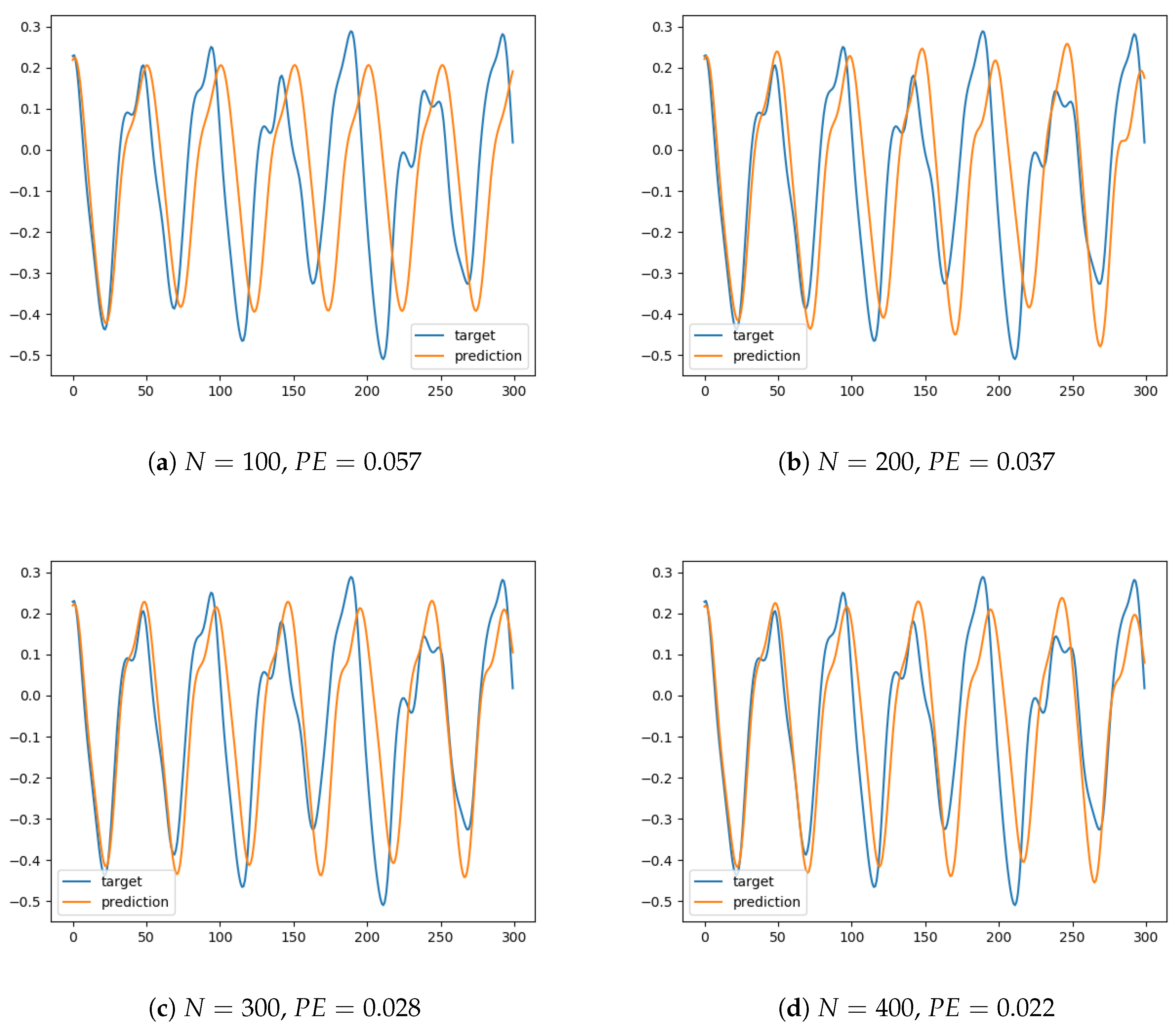
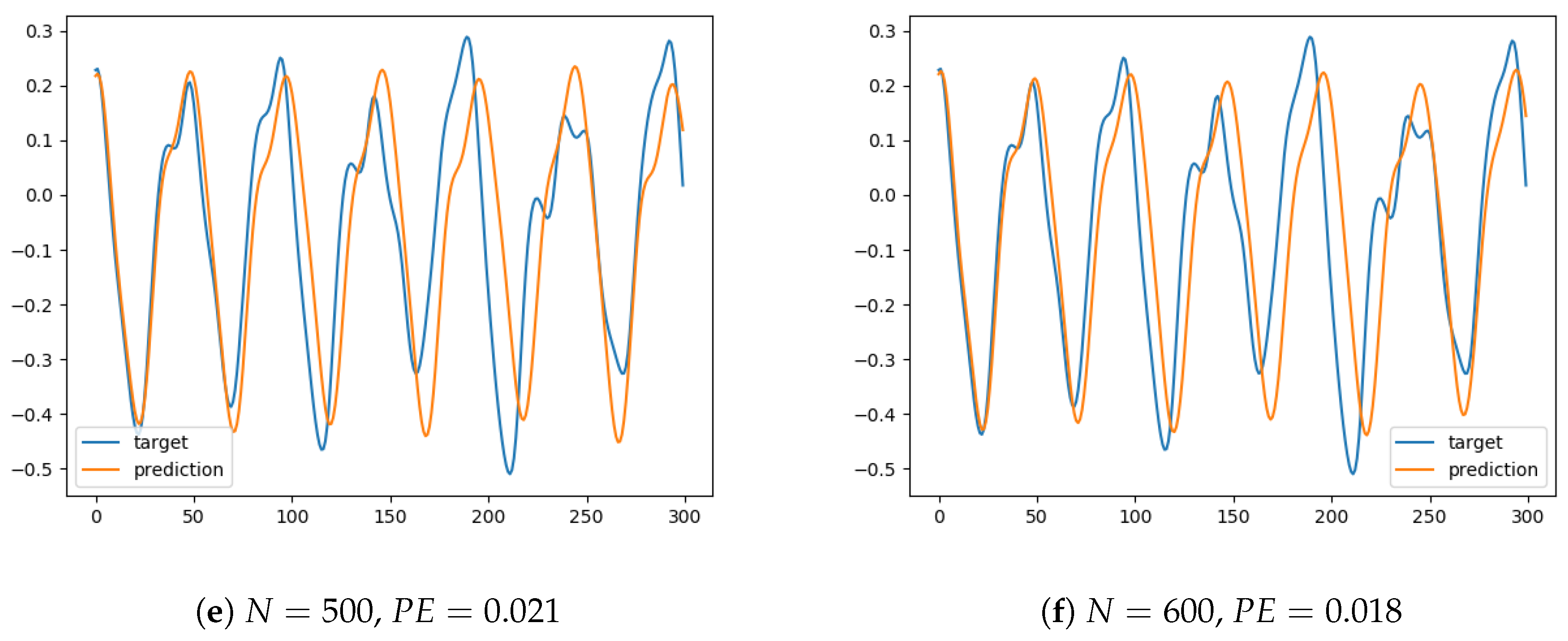
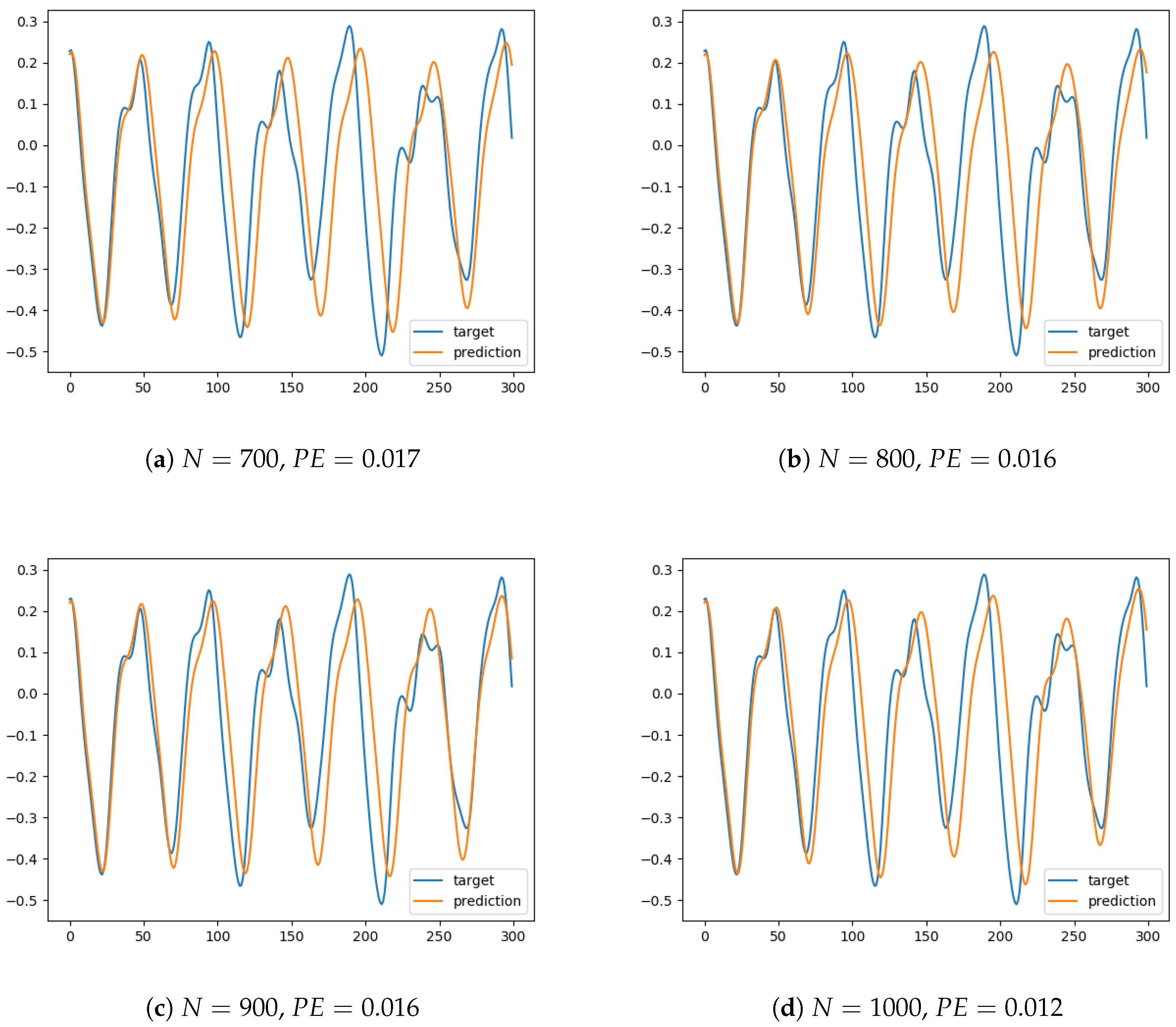
The extensive experiments show that, as expected, prediction accuracy increased with reservoir size. For instance, for a reservoir size $N=100$ (shown in Figure 1a), the prediction soon departed from the target signal and the error increased. Furthermore, the signal seemed to present a delay in oscillations, when compared to the original series. Thus it can be argued that the network was unable to capture thequalitative dynamical behavior of the input. Note that for clarity of exposition we have only plotted a horizon of 300 data points, but other phenomena were observed in the experiments that were performed for longer periods, such as unbounded oscillations or convergence to a constant value—both representing signals with a completely different behavior (from a dynamical systems perspective) to the target signal. In contrast, the simulations for a reservoir size $N=1000$ (Figure 2d) provide a prediction that reasonably fits the target series, with oscillations that are almost synchronized. Additional experiments showed that the ESN was able to generate a similar behavior for longer periods, and thus it can be concluded that it was able to capture the intrinsic nature of the dynamical system.

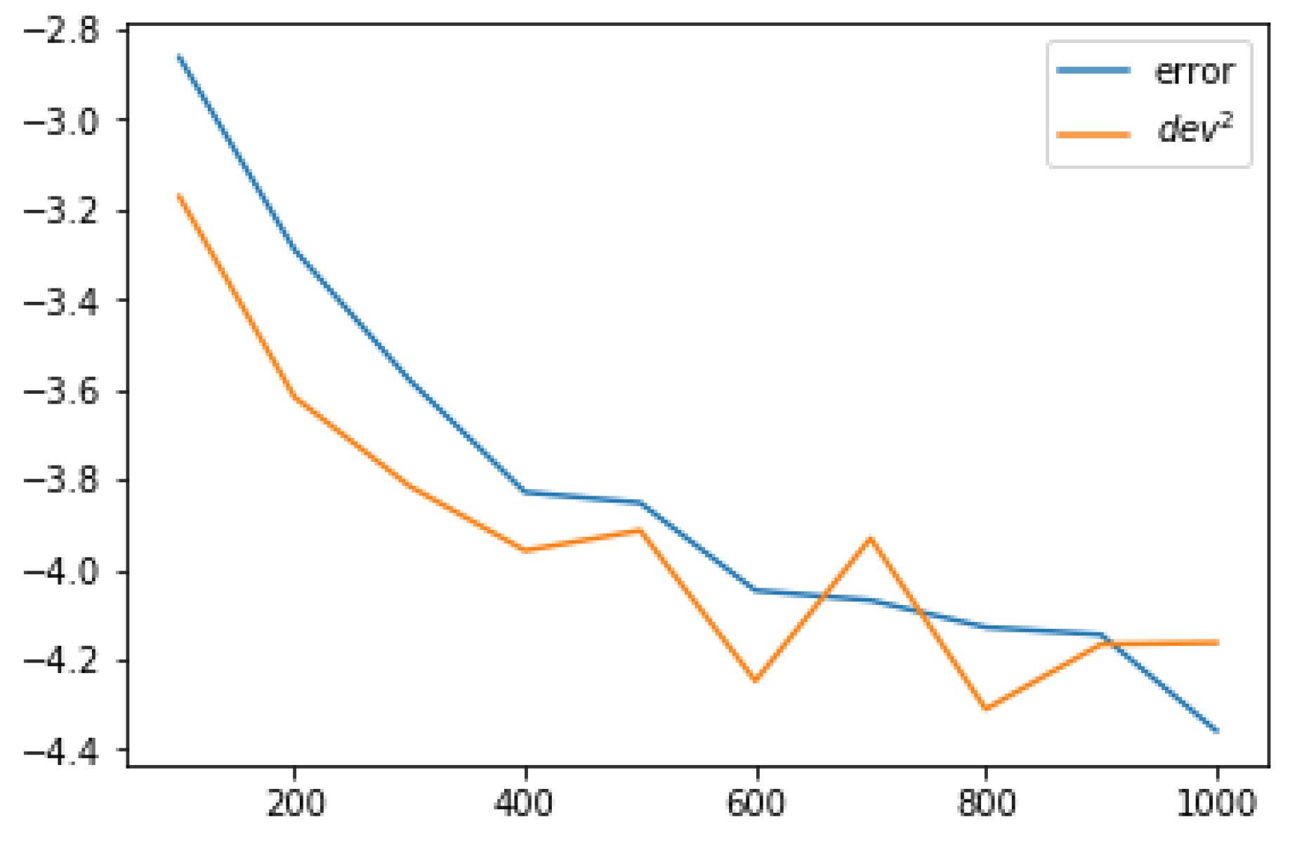
A second set of experiments were performed, with the same basic training and testing scheme. However, in addition to the conventional output prediction provided by the ESN, 100 samples of the output were computed by randomly zeroing a proportion of the units, thus providing a distribution of the outputs. The standard deviation of this distribution was recorded, and then averaged over the 300 data points obtained during the test stage. The obtained results of these average standard deviations for each reservoir size and each value of dropout rate are shown in Table 2. It is clear from these results that when the error was lower (larger reservoir size), the ensemble deviation was also lower. In this way, the ensemble variance could serve as a measure of the reliability of the prediction when the prediction error is not available. This is also illustrated in Figure 3, where both the $PE$ and the computed deviation of the ensemble distribution are shown to present a remarkable similarity (since the $PE$ is a squared error, the deviations are also squared to be comparable; also, both plots are represented in logarithmic scale to enhance the visibility of the slope). It is remarkable that sampling by Monte Carlo dropout is able to grasp the uncertainty inherent to the learning process, even if dropout has not been used during learning, but rather only during the test stage.

One aspect that is subject to empirical research is the determination of the dropout rate that leads to the best assessment of uncertainty. Intuition suggests that when dropout is small, all ensembles would be too similar and the variance would not reflect the uncertainty. Contrarily, a very large dropout rate would lead to the deletion of too many units, so that the error of each individual prediction would be excessive. In order to have an idea of the influence of the dropout rate on the UQ results, we computed the regression between the corresponding column of ensemble deviations for each dropout rate and the prediction error, showing the results in

Table 3. Coefficient of determination $R^2$ when regressing the deviations obtained from the dropout ensembles versus the prediction error, over the different reservoir sizes, for the experiment on the Mackey–Glass equation.

Dropout Rate	${\mathit{R}}^2$
0.1	0.672
0.2	0.785
0.3	0.820
0.4	0.745
0.5	0.401
0.6	0.892
0.7	0.936
0.8	0.846
0.9	0.479

. The maximum correlation was obtained for a dropout rate of 0.7, which is coherent with the above remark about finding a balance between error and variability. In some sense, this can be considered a manifestation of the pervasive bias–variance trade-off.

In order to further assess the information provided by the dropout procedure with regard to the uncertainty of the learning mechanism, we carried out another experiment, using a real-world dataset—namely, the monthly record of sunspots count from 1749 to 2017 [21]. This time series is notoriously difficult to predict because the observed 11-year periodicity only holds approximately. Extensive experimentation to set the hyperparameter values revealed that the ridge regression coefficient $\alpha$ is the most critical parameter, so we focused the cross-validation on this parameter and let the others be fixed as shown in

Table 4. Hyperparameters of the ESN that were kept constant for the experiment on the sunspots dataset.

Parameter Name	Symbol	Value
Spectral radius	$\rho$	0.99
Leaking rate	$\lambda$	0.4
Input scaling	$s_i$	1
Reservoir size	N	1000
Initial transient	$L_{in}$	100
Training length	$L_{tr}$	1000
Test length	$L_{te}$	300
Dropout rate	d	0.7

.

The experiments performed on the sunspot dataset with a dropout rate of $d=0.7$ showed that the prediction performance of the ESN was limited, unlike in the contrived Mackey–Glass equation of the previous experiment set. In

Table 5. Prediction errors and standard deviations of predictions along the dropout ensembles for each value of the ridge coefficient $\alpha$ in the experiment on the sunspot dataset.

Ridge Coefficient	Prediction Error	Deviation through Dropout
$1\times {10}^{-6}$	0.0356	103.4594
$5\times {10}^{-6}$	0.0301	42.3897
$1\times {10}^{-5}$	0.0344	27.7515
$5\times {10}^{-5}$	0.0398	10.6772
$1\times {10}^{-4}$	0.0361	7.2910
$5\times {10}^{-4}$	0.0209	2.9364
$1\times {10}^{-3}$	0.0287	2.0279
$2\times {10}^{-3}$	0.0346	1.3080
$4\times {10}^{-3}$	0.0451	0.8812
$6\times {10}^{-3}$	0.0358	0.7562
$8\times {10}^{-3}$	0.0383	0.6070
$1\times {10}^{-2}$	0.0339	0.5797

, the prediction errors for various values of the ridge coefficient are shown, revealing that the error was fairly independent of the $\alpha$ coefficient. This counter-intuitive behavior suggests that the $PE$, which is just the Euclidean norm of the difference between the series as a whole, does not adequately measure the difference between the series.

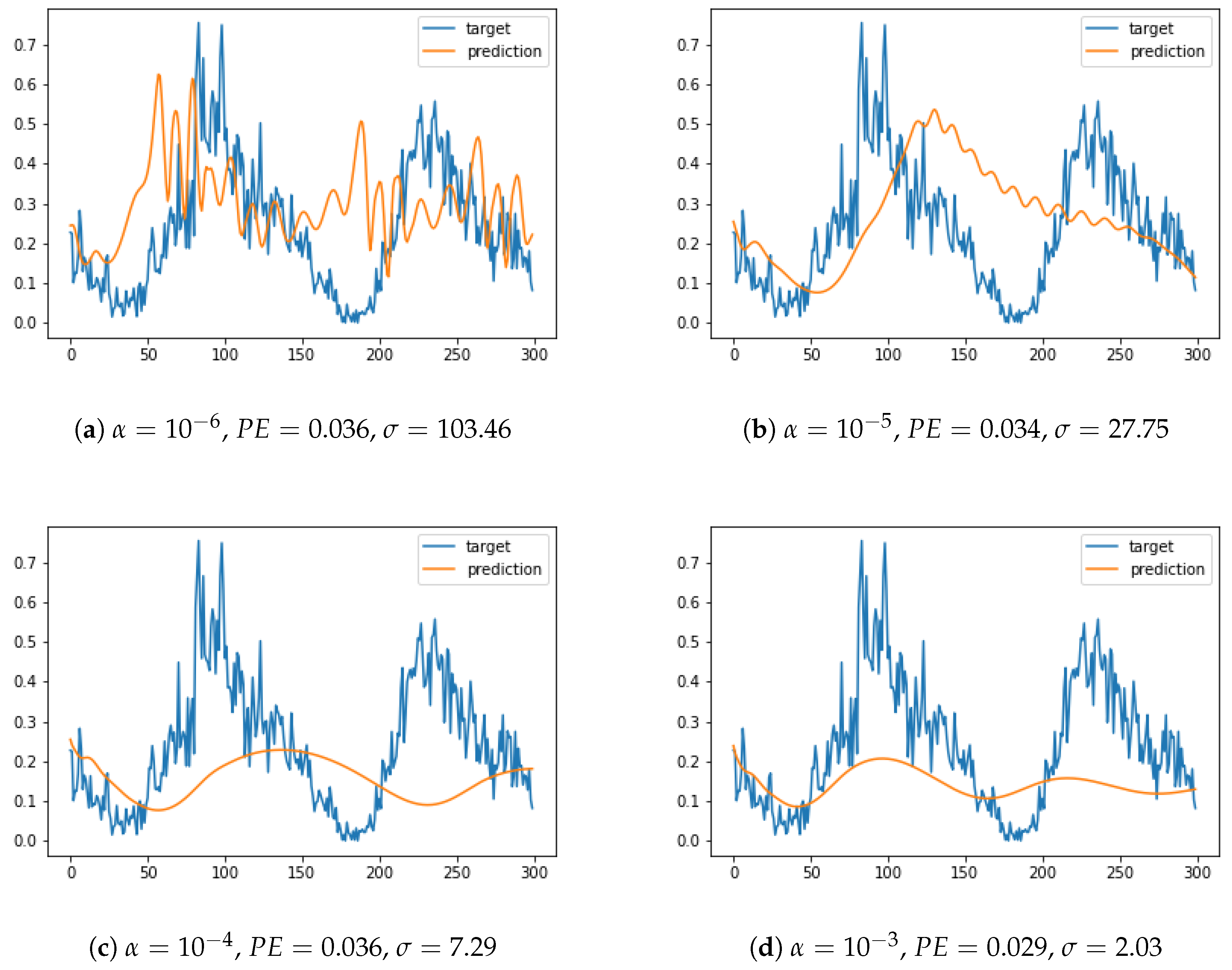
In order to provide a deeper qualitative analysis, in Figure 4 we show the prediction provided by the ESN, compared to the target signal, for various values of the regression coefficient. For instance, for $\alpha ={10}^{-6}$ in Figure 4a it can be clearly observed that the prediction had a completely incorrect qualitative behavior, even though the pointwise difference is not that large: instead of the quasiperiodic signal, a sequence of seemingly chaotic oscillations appears. Correspondingly, the first row of Table 5 contains a very large value of deviation when the prediction was repeated with many ESNs with some units removed. In other words, the uncertainty quantification mechanism proposed in this paper was able to recognize a dubious prediction from the dynamical point of view of the time series, even though the prediction error failed to do so. In contrast, in Figure 4d, which corresponds to a value $\alpha =0.01$, the prediction is qualitatively similar to the target, at least regarding the first peak and the general trend. Intermediate behaviors can be observed in Figure 4b,c, ranging from damped oscillations to a delay. This progressive improvement of the prediction from a qualitative, dynamical point of view is adequately captured by the decrease of the deviation of the dropout ensembles, as shown in Table 5.

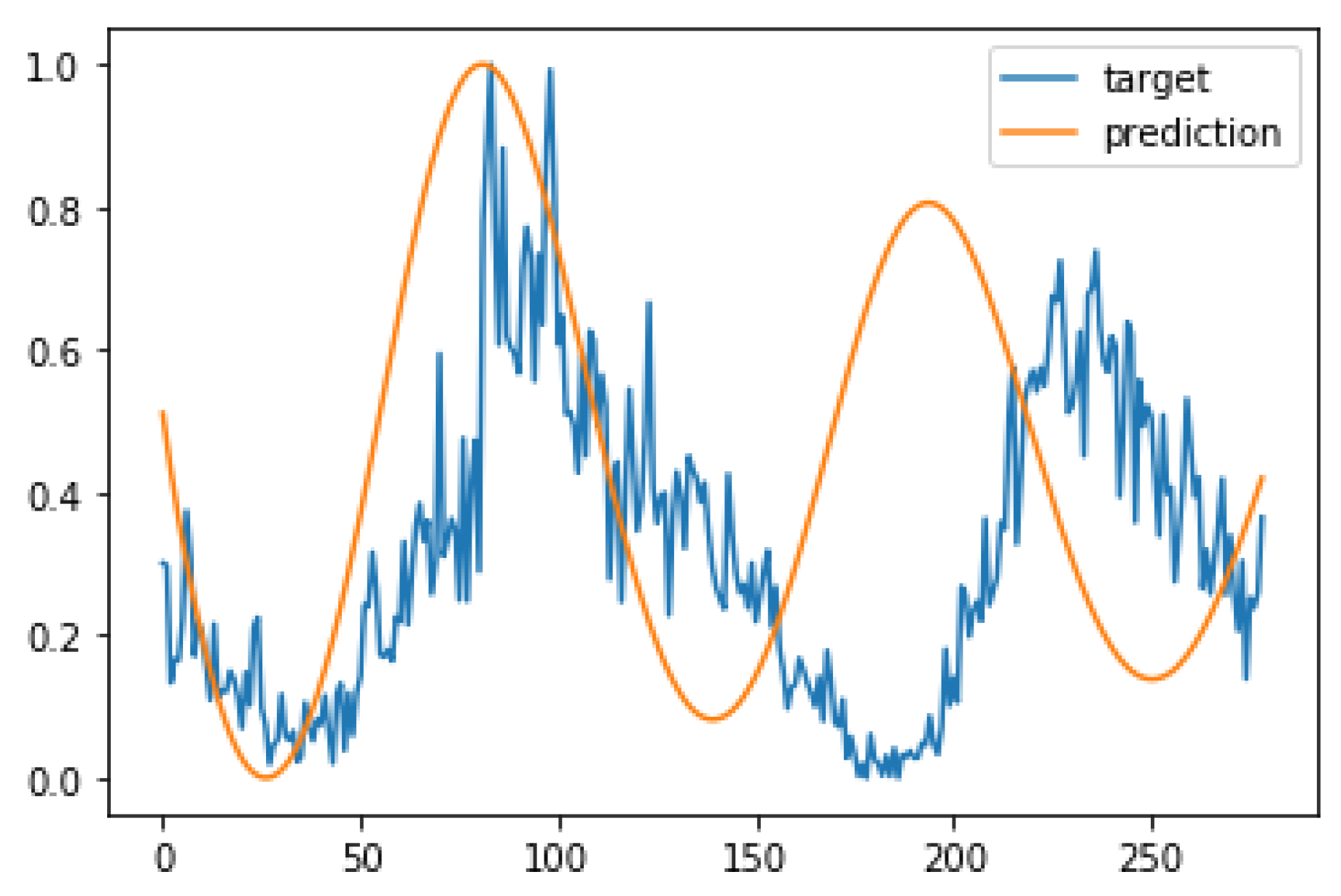
As a first step in the formalization of the qualitative remarks of the previous paragraph, we reproduced Figure 4d corresponding to $\alpha =0.01$ (i.e., the lowest value of the dropout deviation d). However, we rescaled and shifted the prediction so the fist peak matches that in the original series. The result is shown in Figure 5, where a recognizable similarity can be clearly seen. This result suggests that the error measured as the Euclidean distance between vectors did not adequately measure whether the series shared similar dynamical features, since it disregards the temporal relations. In this sense, we propose as an interesting direction for further research the exploration of other time series distances (see [22] and references therein), and its use in the learning mechanism of the ESN.

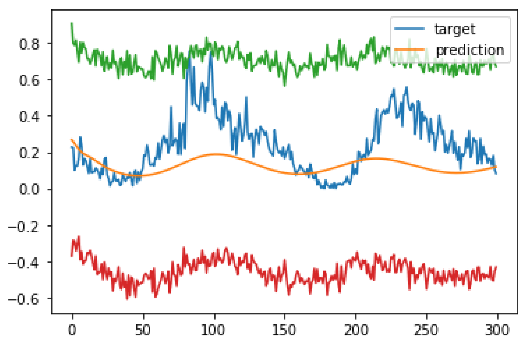
Finally, we obtain further insight in the uncertainty information provided by the dropout procedure in Figure 6, which again represents the prediction on the sunspot series for $\alpha =0.01$. However, in this case we have added two lines resulting from the addition and subtraction of the dropout deviation to and from the base prediction. The fact that the correct series values lie within this interval suggests a mechanism for robust prediction that deserves future research.

5. Conclusions

In this work we presented a mechanism to assess the accuracy of prediction of time series by echo state networks. The procedure is based upon the repeated sampling of the outputs obtained when a percentage of units are dropped out. In this way, we construct an empirical distribution of the outputs, from which a measure of uncertainty can be obtained (e.g., by recording the standard deviation of such distribution). When the ESN achieved good learning results, experiments showed that the deviation of the dropout deviation was consistently correlated with the prediction error, thus serving as a mechanism for uncertainty quantification. In contrast, for a complex real-world dataset, prediction performance was limited. In this case, the prediction error was not an accurate measure of series similarity. However, low values of the dropout deviation correspond to qualitatively correct dynamical features, even though much work is needed to formally quantify this phenomenon.

Note that the dropout procedure was only used for UQ during the test stage, rather than the more usual application as a method for the prevention of overfitting during training. Incidentally, in some experiments not shown here for brevity, we determined that the average of the distribution of dropout samples was remarkably similar to the direct output; thus, the latter seems to be an unbiased estimator of the target value. However, in generative (test) mode, since the output is fed back to the input, driving the network dynamics, even this small difference could lead to a qualitatively different dynamical behavior. This suggests a line for future research aimed at improving the prediction performance of the ESN, by using as predicted output the average (or even other statistic) of the distribution that is obtained from the repeated samplings with dropout. The obvious next step would be to use dropout also during training—a method that is intuitively supported by the idea that learning should happen in a situation as similar as possible as the one where recall is intended. This could be combined with the exploration of other choices of parameter values, particularly the ridge coefficient. Additionally, variants of learning that have shown improved results, such as those in [23], are being explored. Finally, the use of alternative measures, beyond the Euclidean distance, is worth considering both in the training and test phases.

References

- Zhang, G.P. Neural networks for time-series forecasting. In Handbook of Natural Computing; Springer: Berlin/Heidelberg, Germany, 2012; Volume 1–4, pp. 461–477. [Google Scholar]
- Watt, N.; Du Plessis, M.C. Dropout algorithms for recurrent neural networks. In Proceedings of the ACM International Conference Proceeding Series. Association for Computing Machinery, Beijing, China, 24–25 October 2018; pp. 72–78. [Google Scholar]
- Bacciu, D.; Crecchi, F. Augmenting Recurrent Neural Networks Resilience by Dropout. IEEE Trans. Neural Netw. Learn. Syst. 2020, 31, 345–351. [Google Scholar] [CrossRef] [PubMed]
- McDermott, P.L.; Wikle, C.K. An ensemble quadratic echo state network for non-linear spatio-temporal forecasting. Stat 2017, 6, 315–330. [Google Scholar] [CrossRef] [Green Version]
- McDermott, P.L.; Wikle, C.K. Deep echo state networks with uncertainty quantification for spatio-temporal forecasting. Environmetrics 2019, 30, e2553. [Google Scholar] [CrossRef] [Green Version]
- Sheng, C.; Zhao, J.; Wang, W.; Leung, H. Prediction intervals for a noisy nonlinear time series based on a bootstrapping reservoir computing network ensemble. IEEE Trans. Neural Netw. Learn. Syst. 2013, 24, 1036–1048. [Google Scholar] [CrossRef] [PubMed]
- Jaeger, H.; Lukoševičius, M.; Popovici, D.; Siewert, U. Optimization and applications of echo state networks with leaky- integrator neurons. Neural Netw. 2007, 20, 335–352. [Google Scholar] [CrossRef] [PubMed]
- Hochreiter, S.; Schmidhuber, J. Long Short-Term Memory. Neural Comput. 1997, 9, 1735–1780. [Google Scholar] [CrossRef] [PubMed]
- Lukoševičius, M. A Practical Guide to Applying Echo State Networks. In Neural Networks: Tricks of the Trade; Montavon, G., Orr, G.B., Muller, K.R., Eds.; Springer: Berlin/Heidelberg, Germany, 2012; Volume 7700, pp. 659–686. [Google Scholar]
- Gallicchio, C.; Micheli, A. Echo state property of deep reservoir computing networks. Cogn. Comput. 2017, 9, 337–350. [Google Scholar] [CrossRef]
- Srivastava, N.; Hinton, G.; Krizhevsky, A.; Sutskever, I.; Salakhutdinov, R. Dropout: A Simple Way to Prevent Neural Networks from Overfitting. J. Mach. Learn. Res. 2014, 15, 1929–1958. [Google Scholar]
- Gal, Y.; Ghahramani, Z. Dropout as a Bayesian Approximation: Representing Model Uncertainty in Deep Learning. In Proceedings of the 33rd International Conference on Machine Learning—Volume 48. JMLR.org, ICML’16, New York, NY, USA, 20–22 June 2016; pp. 1050–1059. [Google Scholar]
- Wickstrøm, K.; Kampffmeyer, M.; Jenssen, R. Uncertainty and interpretability in convolutional neural networks for semantic segmentation of colorectal polyps. Med. Image Anal. 2020, 60, 101619. [Google Scholar] [CrossRef] [PubMed]
- Myojin, T.; Hashimoto, S.; Mori, K.; Sugawara, K.; Ishihama, N. Improving Reliability of Object Detection for Lunar Craters Using Monte Carlo Dropout. In Proceedings of the ICANN, Munich, Germany, 17–19 September 2019; Volume 11729, pp. 68–80. [Google Scholar]
- Kim, Y.C.; Kim, K.R.; Choe, Y.H. Automatic myocardial segmentation in dynamic contrast enhanced perfusion MRI using Monte Carlo dropout in an encoder-decoder convolutional neural network. Comput. Methods Programs Biomed. 2020, 185, 105150. [Google Scholar] [CrossRef] [PubMed]
- Zhu, L.; Laptev, N. Deep and Confident Prediction for Time Series at Uber. In Proceedings of the 2017 IEEE International Conference on Data Mining Workshops (ICDMW), New Orleans, LA, USA, 18–21 November 2017; pp. 103–110. [Google Scholar]
- Elola, A.; Aramendi, E.; Irusta, U.; Picón, A.; Alonso, E.; Owens, P.; Idris, A. Deep Neural Networks for ECG-Based Pulse Detection during Out-of-Hospital Cardiac Arrest. Entropy 2019, 21, 305. [Google Scholar] [CrossRef] [Green Version]
- Wen, H.; Gu, J.; Ma, J.; Jin, Z. Probabilistic Wind Power Forecasting via Bayesian Deep Learning Based Prediction Intervals. In Proceedings of the 2019 IEEE 17th International Conference on Industrial Informatics (INDIN), Helsinki, Finland, 22–25 July 2019; Volume 1, pp. 1091–1096. [Google Scholar]
- Stoean, R.; Stoean, C.; Abdar, M.; Atencia, M.; Velázquez-Pérez, L.; Khosravi, A.; Nahavandi, S.; Acharya, U.R.; Joya, G. Automated Detection of Presymptomatic Conditions in Spinocerebellar Ataxia Type 2 using Monte-Carlo Dropout and Deep Neural Network Techniques with Electrooculogram Signals. Sensors 2020, 20, 3032. [Google Scholar] [CrossRef] [PubMed]
- Stoean, R.; Stoean, C.; Atencia, M.; Rodríguez-Labrada, R.; Joya, G. Ranking Information Extracted from Uncertainty Quantification of the Prediction of a Deep Learning Model on Medical Time Series Data. Mathematics 2020, 8, 1078. [Google Scholar] [CrossRef]
- Seabold, S.; Perktold, J. statsmodels: Econometric and statistical modeling with python. In Proceedings of the 9th Python in Science Conference, Austin, TX, USA, 28 June–3 July 2010. [Google Scholar]
- Jiang, G.; Wang, W.; Zhang, W. A novel distance measure for time series: Maximum shifting correlation distance. Pattern Recognit. Lett. 2019, 117, 58–65. [Google Scholar] [CrossRef]
- Jaeger, H.; Haas, H. Harnessing nonlinearity: Predicting chaotic systems and saving energy in wireless communication. Science 2004, 304, 78–80. [Google Scholar] [CrossRef] [Green Version]
Figure 1.
Prediction for values of the reservoir size from to , showing the prediction error ().
Figure 2.
Figure 3.
Prediction error and squared dropout ensemble deviation, both in logarithmic scale, for a dropout rate , in the experiment on the Mackey–Glass equation.
Figure 4.
Prediction for different values of the ridge regression coefficient α for the sun spots dataset, showing the prediction error and the dropout ensemble deviation σ.
Figure 5.
Normalized and shifted prediction for the sunspot dataset.
Figure 6.
Prediction for the sunspot dataset with . Two plots have been added to represent the dropout deviation as an interval around the conventional output.