Optimization Parameters of Trading System with Constant Modulus of Unit Return

Abstract

The unit return is determined as the return in the quotation currency (QCR) per the unit of base exchange medium (BEM). The main purpose is to examine the applicability of a trading system with a constant modulus of unit return (CMUR). The CMUR system supports speculative operations related to the exchange rate, given as the BEM quotation per the QCR. Premises for investment decisions are based on knowledge about the quotation dynamics described by its binary representation. This knowledge is described by a prediction table containing the conditional probability distributions of exchange rate increments. Any prediction table depends on observation range. Financial effectiveness of any CMUR system is assessed in the usual way by interest rate and risk index based on Shannon entropy. The main aim of our paper is to present algorithms which may be used for selecting effective CMUR systems. Required unit return modulus and observation range are control parameters applied for management of CMUR systems. Optimal values of these parameters are obtained by implementation of the proposed algorithm. All formal considerations are illustrated by an extensive case study linked to gold trading.

1. Introduction

Each financial instrument is determined as a given asset in short position or in long position. The speculator’s earning does not result from the underlying asset attributes, such as long-term technical analysis or fundamental ratios. In general, speculation is the acquisition of a financial instrument with the expectation that it will be sold as more expensive in the near future [1]. Therefore, speculation is acquisition of an asset in anticipation of its price increase, and also the disposal of an asset in anticipation of its price fall. For these reasons, speculation transaction is such financial transactions where the speculator’s earnings result from short-term fluctuations in the quoted price of a traded asset. For these reasons, speculation transactions can only be implemented on financial markets characterized by frequent price changes. Moreover, the duration of a single speculative transaction is generally short. This is why speculation transactions require the use of High-Frequency Trading (HFT) systems. HFT systems help traders hold positions for short periods of time and earn their profits by accumulating tiny gains on a large number of transactions [2].

The existing body of literature on HFT is extensive, and it covers many items devoted to different aspects of HFT [2,3]. IT techniques’ development implies an increase in HFT systems’ popularity.

The subject of speculation is trading in base exchange medium (BEM), given as any currency, any precious metal, or any standardized commodity. All speculative transactions are related to an exchange rate, given as the BEM quotation per the quotation currency (QCR). The trading in exchange rates is organized on the Foreign eXchange market (FX), characterized by very frequent price changes. Therefore, speculative transactions are implemented on FX. A price dynamic on FX may be characterized by unite return, defined as the return in QCR per unit of BEM [4].

Generally, financial speculators use well-known methods to manage speculative transactions. On the other hand, most speculators bear losses [5,6]. The above fact shows that this is not a good approach to profitable trading. Hence, there is demand for a new, fully justified method of financial market analyses supporting speculative transactions [7].

Among other things, heuristic trading systems are used on financial markets [8,9]. On the other hand, applied mathematics is the obvious research field for new HFT systems. For example, here, we use advanced mathematical statistics [10,11,12], genetic algorithms [13,14,15], artificial intelligence models [11], neural networks [16,17,18,19,20,21], multi agent theory [10,22,23], and mathematics for fuzzy systems [10]. Applying these theories requires acceptance of strong formal assumptions. Therefore, the mathematical apparatus used significantly limits the field of practical applications. This causes a demand for such HFT systems that their mathematical models are based on weak formal assumptions.

An HFT system may be determined with use of the criterion of Constant Modulus of Return Rate (CMUR) [4]. To the best of our knowledge, proposing CMUR systems in 2019 is completely original. For this reason, the CMUR systems’ bibliography contains only Reference [4] and a few pilot studies [24,25,26,27,28,29,30,31,32].

The correct application of the CMUR system requires only a few general assumptions. Moreover, the CMUR system is very basic. Therefore, applied mathematical apparatus does not significantly restrict the area of CMUR system use. In previous pilot studies [23,24,25,26,27,28,29,30,31,32], the necessary mathematical assumptions were always met, and this is a very important advantage of the CMUR system.

Aldridge [7] distinguish the following FX participants: high-frequency speculators, long-term investors, and corporations. The CMUR system can support speculators. Any HFT system can consist of three components: transaction management, risk reduction, and money management [33,34]. The CMUR system does not refer to money management, which is a disadvantage of the CMUR system.

Any HFT system is related to the method of financial prediction [2,10,35,36,37,38,39]. In the CMUR system, a sign of unitary return is forecasted with the use of a simple prediction table specified for required unitary return modulus on the space of all binary states of an assumed observation range. In this way, required unitary return modulus and assumed states observation range are the only control parameters of the CMUR system. It means that any CMUR system is uniquely determined by the fixed pair of control parameters.

The application of the CMUR system each time requires choice of the optimal variant of its control parameters. This selection is made by the speculator. The main goal of this paper is presentation of a method of optimization control parameters of the CMUR system. Any variant of control parameters will be evaluated by the ex-ante characteristic proposed in Reference [4]. Optimal variants of the control parameters system will be chosen as the Pareto set.

The article is organized in the following way. Section 2 describes the procedure of discretization Ask price trend. Here, we simplify the procedure description given in Reference [4]. We obtained this simplification in this way by omitting all the proofs and justifications required in Reference [4]. In an analogous way, we simplified the description of the CMUR model, as presented in Section 3. In Section 4, we present some tools for assessing financial effectiveness of CMUR systems. In Section 5, we propose original algorithms that select the optimal variants of the CMUR system. In Section 6, obtained theoretical results are illustrated by an extensive case study linked to gold trading. Section 7 justifies the ambiguity of the obtained results and points to the future research directions.

2. Discretization of Ask Price Trend

By basic exchange medium (BEM), we understand any base currency, any precious metal, or any standardized commodity. On the financial market of the exchange pair BEM/QCR, each considered BEM price is expressed in the quoted currency (QCR). The exchange pair BEM/QCR market is also called the BEM/QCR market. The Ask price of BEM is the unit price of BEM in the QCR. In each moment of time, $t\in \left[0,T\right]$, we note the Ask price, $Q_{Ask}\left(t\right)$. In this way, we determine the Ask price trend, $Q_{Ask}:\left[0,T\right]\to {ℝ}^{+}$, which describes the dynamics of an exchange pair, BEM/QCR.

In this section, we describe such method of discretization Ask price trend, which is dedicated to CMUR systems. This discretization method was introduced and justified in Reference [4]. The changes on the BEM/QCR market are described by a unit return, defined as a dirty return by the BEM amount. The unit return $𝓊𝓇\left(t^{\prime },t^{″}\right)$ in the time interval $\left[t^{\prime },t^{″}\right]$ equals

$$𝓊𝓇\left(t^{\prime },t^{″}\right)=Q_{Ask}\left(t^{″}\right)-Q_{Ask}\left(t^{\prime }\right).$$

(1)

In the first step, we create a binary representation of Ask price trend. Applied binary representation is inspired by the historical point-symbolic notation [40].

We observe a continuous trend, $Q_{Ask}:\left[0,T\right]\to {ℝ}^{+}$. If a single trend observation begins at the time $t^{\prime }$, then it ends as early as possible at the moment $t^{″}>t^{\prime }$, fulfilling condition

$$\left|𝓊𝓇\left(t^{\prime },t^{″}\right)\right|=\delta >0$$

(2)

where $\delta$ is assumed as the discretization unit. We must remember that the assumed discretization unit, $\delta ,$ should be equal to the unit return modulus requested by the speculator.

The event, ${ℐ}_{\delta },$ denotes such an Ask price increase which fulfils the condition (2). The complement, ${ℐ}_{\delta }^C,$ of this event is Ask price fall fulfilling condition (2). Forecasting changes in the Ask price is limited to answering the question of whether there will be an increase, ${ℐ}_{\delta }$, or a decrease, ${ℐ}_{\delta }^C,$ after the current time, $t^{\prime }$. The examined CMUR systems require only such elementary forecasts.

The first trend observation begins at the time $t_0=0$. We assume that the observation continuity of it means that at each moment of closing the observation, the next observation is opened. That is why the sequence, ${\left(t_i\right)}_{i=0}^n\subset \left[0,T\right],$ of observation opening moments is recursively determined in the following way:

$$t_0=0,$$

(3)

$$t_{i+1}=\min \left\{\min \left\{\tau >t_i:𝓊𝓇\left(t_i,\tau \right)=\delta \right\},\min \left\{\tau >t_i:𝓊𝓇\left(t_i,\tau \right)=-\delta \right\}\right\}.$$

(4)

The sequence ${\left(t_i\right)}_{i=0}^n$ is a record of the observation history. Therefore, the sequence ${\left(t_i\right)}_{i=0}^n=\mathsf{\Theta }$ is called an observation record.

The binary representation of the trend $Q_{Ask}:\left[0,T\right]\to {ℝ}^{+}$ consists of transforming this trend into its binary representation $ℰ={\left({\epsilon }_i\right)}_{i=1}^n,$ determined as follows:

$${\epsilon }_i=\{\begin{array}{c}1 𝓊𝓇\left(t_{i-1},t_i\right)=\delta \\ 0 𝓊𝓇\left(t_{i-1},t_i\right)=-\delta \end{array}.$$

(5)

The number, $n,$ of binary observations contained in the binary representation $ℰ={\left({\epsilon }_i\right)}_{i=1}^n$ depends on the discretization unit $\delta$ and the length $T$ of the observation interval.

For set observation range $c\in \mathbb{N}$, we define the state space ${\mathbb{E}}_c$ as the set of all c-elements’ permutations with repetition from the set $\left\{0, 1\right\}$. The state space ${\mathbb{E}}_c$ consists of $2^c$ states defined in the following way:

$${\mathrm{s}}_j=\left(e_1,e_2,\dots ,e_c\right),$$

(6)

where

$$j={\displaystyle \sum }_{l=1}^c{2}^{c-l}{e}_l+1$$

(7)

The observation range $c\in \mathbb{N}$ is chosen by an analyst examining the BEM/QCR market. We will use any state $s_j\in {\mathbb{E}}_c$ as as the only premise for the forecast required by the CMUR system.

Example 1

[4]. For the number $c=4$, we have the following state space:

$${\mathbb{E}}_4=\left\{\begin{array}{c}{s}_1=\left(0,0,0,0\right), s_2=\left(0,0,0,1\right), s_3=\left(0,0,1,0\right),s_4=\left(0,0,1,1\right),\\ s_5=\left(0,1,0,0\right), s_6=\left(0,1,0,1\right),s_7=\left(0,1,1,0\right),s_8=\left(0,1,1,1\right),\\ s_9=\left(1,0,0,0\right),s_{10}=\left(1,0,0,1\right), s_{11}=\left(1,0,1,0\right), s_{12}=\left(1,0,1,1\right),\\ s_{13}=\left(1,1,0,0\right), s_{14}=\left(1,1,0,1\right), s_{15}=\left(1,1,1,0\right), s_{16}=\left(1,1,1,1\right),\end{array}\right\}.$$

(8)

Let us take into account fixed binary representation $ℰ={\left({\epsilon }_i\right)}_{i=1}^n$ associated with observation record $\mathsf{\Theta }$. Each moment $t_i\in \mathsf{\Theta } \left(i=c, c+1,\dots ,n\right)$ is attributed to an observed state, ${\tilde{s}}_i\in {\mathbb{E}}_c,$ of the BEM/QCR market. In this way, we create a sequence,

$$\Xi ={\left({\tilde{s}}_i\right)}_{i=c}^n={\left({\left({\epsilon }_k\right)}_{k=i-c+1}^i\right)}_{i=c}^n,$$

(9)

of following observations of market states. The sequence, $\Xi ,$ defined in this way is a record of all observed changes in BEM/QCR market states. Therefore, the sequence, $\Xi ,$ is called a state record.

For any pair, $\left(t_i,t_{i+1}\right)\subset \mathsf{\Theta }$, the value ${\epsilon }_{i+1}=1$ denotes the observation of rise in the Ask price in the interval $\left[t_i,t_{i+1}\right]$. Then, the value ${\epsilon }_{i+1}=0$ denotes the observation of fall in the Ask price in the interval $\left[t_i,t_{i+1}\right]$. For the purposes of Ask price trend discretization, the sequence

$$\Psi ={\left(\tilde{s}\left(t_i\right),{\epsilon }_{i+1}\right)}_{i=c}^{n-1}$$

(10)

plays the role of a training dataset [41].

Each state, $s_j\in {\mathbb{E}}_c,$ is observed exactly $n_j$ times. The sequence ${\left(n_j\right)}_{j=1}^{2^c }$ of random numbers is explicitly determined by training dataset $\Psi$. Thanks to this, for each $j=1,2,\dots ,m,$ we can establish the probability

$$p\left(s_j\right)=\frac{n_j}{n-c-1}$$

(11)

of achieving the state $s_j$. Moreover, the training dataset $\Psi$ determines the space of all observed states

$${\mathbb{G}}_c\left(\Psi \right)=\left\{s_j\in {\mathbb{E}}_c: n_j>0\right\}.$$

(12)

In Reference [4] it is justified that the training dataset $\Psi$ uniquely determines conditional probability

$$p\left({ℐ}_{\delta }|s_j\right)=\frac{n_j^{*}}{n_j},$$

(13)

of achieving assumed rise, ${ℐ}_{\delta },$ immediately after that the state, $s_j,$ has occurred. The sequence ${\left(n_j^{*}\right)}_{j=1}^m$ is explicitly determined as follows:

$$n_j^{*}={{\displaystyle \sum }}_{\left\{i: c\le i\le n-c-1, {\tilde{s}}_i=s_j\right\}}^{}{\epsilon }_i$$

(14)

The total probability, $p\left({ℐ}_{\delta }\right),$ of rise in Ask price can be determined as:

$$p\left({ℐ}_{\delta }\right)={\displaystyle \sum }_{s_j\in {\mathbb{G}}_c\left(\Psi \right)}p\left(s_j\right)·p\left({ℐ}_{\delta }|s_j\right).$$

(15)

The set of triples below:

$$𝒫(\mathrm{BEM}/\mathrm{QCR},\delta ,c,\Psi )=\left\{\right(n_j,p\left(s_j\right),p\left({ℐ}_{\delta }|s_j\right)):s_j\in {\mathbb{G}}_c\left(\Psi \right)\},$$

(16)

forms the prediction table to foresee the changes of the BEM/QCR exchange rate For any exchange pair BEM/QCR, its prediction table depends only on three parameters:

• $\Psi$—training dataset,
• $\delta$—discretization unit,
• $c$—observation range.

The training dataset $\Psi$ depends on observed ex-ante Ask price trend, $Q_{Ask}:\left[0,T\right]\to {ℝ}^{+}$, on required discretization unit, $\delta$, and on assumed observation range, $c$. During the calculation of the prediction table, financial analysts and traders do not have influence on the observed ex-ante Ask price trend. Therefore, training dataset $\Psi$ cannot be taken into account as a control parameter of a prediction table.

On the other hand, discretization unit, $\delta$, and observation range, $c,$ are always specified by financial analysts and traders. Therefore, these last two parameters may be considered as control ones.

The confidence interval of a sample statistic (13) is given as the Wald confidence interval [42]. The proposed approximation is reliable when the sample size is large enough, and the success probability is noticeably different from 1 [43].

The value $\alpha$ is the assumed value of a significance level. For each state, $s_j\in {\mathbb{G}}_c\left(\Psi \right)$, the $\left(1-2·\alpha \right)$ level Wald’s confidence interval is given by the equation

$$\begin{gathered} {\mathbb{W}}_j\left(\alpha \right)=\left[p\left({ℐ}_{\delta }|s_j\right)-z_{\alpha }·\sqrt{\frac{p\left({ℐ}_{\delta }|s_j\right)\left(1-p\left({ℐ}_{\delta }|s_j\right)\right)}{n_j}},p\left({ℐ}_{\delta }|s_j\right)+z_{\alpha } \\ ·\sqrt{\frac{p\left({ℐ}_{\delta }|s_j\right)\left(1-p\left({ℐ}_{\delta }|s_j\right)\right)}{n_j}},\right] \end{gathered}$$

(17)

where $z_{\alpha }$ is the $\alpha${\displaystyle 1-{\tfrac {\alpha }{2}}} quantile of a standard normal distribution. In financial practice, the minimal sample size should be determined empirically.

Each state, $s_j\in {\mathbb{E}}_c,$ can use a prediction premise. If prediction premise $s_j\in {\mathbb{E}}_c$ fulfils the condition

$$\left\{1-p\left({ℐ}_{\delta }|s_j\right)\right\}\notin {\mathbb{W}}_j\left(\alpha \right),$$

(18)

then it is called a well-justified premise. Other prediction premises are called ill-justified ones. In this way, for assumed $\alpha$ level of significance, we determine the space,

$$\mathbb{D}\left(\alpha ,\delta , c\right)=\left\{s_j\in {\mathbb{G}}_c\left(\Psi \right): \left\{1-p\left({ℐ}_{\delta }|s_j\right)\right\}\notin {\mathbb{W}}_j\left(\alpha \right)\right\},$$

(19)

of all well-justified premises. For any well-justified premise, the probability of inaccurate forecasting Ask price change is not greater than the value $\alpha$. For ill-justified premises, this probability increases. Therefore, when it is possible, ill-justified premises should be avoided.

In practice, FX is the main financial market where the BEM/QCR exchange rate is traded. All quotations on the FX are related to the BEM unit. For any base currency (BCR) except Japanese Yen (JPY), the BEM unit equals to its monetary unit. For JPY, the BEM unit is equal to 100 JPY. For any precious metal, the BEM unit is equal to 1 troy ounce (1 oz). Major precious metals traded in the FX are gold, marked by acronym XAU, and silver, marked by acronym XAG.

On the FX, traders use the lot as a measure unit for the BEM amount.

Table 1. Lot definitions for main base exchange mediums (BEMs).

BEM	Lot Size
BCR	100,000 BEM units
XAU	100 oz
XAG	1000 oz

contains different lot values determined for various BEMs.

In FX, a change in an exchange rate is expressed in pips. One pip is equal to 0.0001 lot of QCR.

Example 2

[4]. We discuss some cases of speculations in exchange pair silver quoted in U.S. dollars (XAG/USD). The selected value, $\delta =28 pips,$ of assumed discretization unit is justified in Reference [28]. We use the space ${\mathbb{E}}_4$ of all possible FX states.

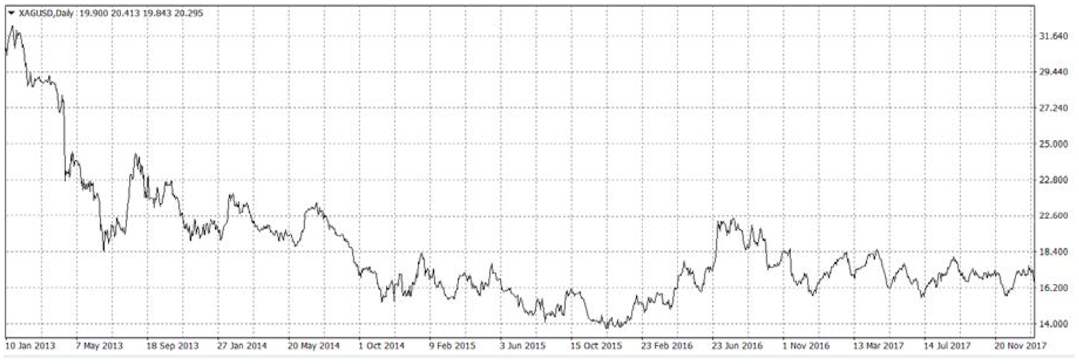
In the first research stage, we determine the prediction table and distinguish well-justified premises. The Dukascopy broker has collected tick data containing 42,782,438 XAG/USD quotations from 31 December 2012 to 1 January 2018, denoted in the following way: $\left[0, 5Y\right]$. For exchange pair XAG/USD, these tick data determine the Ask price trend, $Q_{Ask}:\left[0,5Y\right]\to {ℝ}^{+}$. This trend graph is presented in Figure 1.

We see that the trend $Q_{Ask}$ contains descriptions of bull market, bear market rand, and sideways market. For this reason, we can say that collected tick data are representative.

Using recurrent Formula (4), we transform the collected tick data into the observation record $\Theta ={\left(t_i\right)}_{i=0}^{1480}\subset \left[0,5Y\right]$. In the next step, with Formula (5), we set binary representation$ℰ={\left\{{\epsilon }_i\right\}}_{i=1}^{1480}$of Ask price trend $Q_{Ask}$.

The binary representation $ℰ$ is applied for determination of the state record $\Xi ={\left({\tilde{s}}_i\right)}_{i=4}^{1480}={\left({\left({\epsilon }_k\right)}_{k=i-3}^i\right)}_{i=4}^{1480}$. Taking together all the above results, we build training dataset $\Psi ={\left(\tilde{s}\left(t_i\right),{\epsilon }_{i+1}\right)}_{i=4}^{1479},$ which is used for calculation of the prediction table $𝒫(XAG/USD,28,4,\Psi )$ presented in

Table 2. Prediction table $𝒫(XAG/USD,28,4,\Psi )$ and Wald confidence intervals.

$s_j$		$p\left(s_j\right)$	$p\left({ℐ}_{28}|s_j\right)$	${\mathbb{W}}_j\left(0.05\right)$
$s_1^{\#}$	96	0.065085	0.4688	$\left[0.385272, 0.552328\right]$
$s_2$	87	0.058983	0.4205	$\left[0.333705, 0.507295\right]$
$s_3$	101	0.068475	0.5941	$\left[0.513965, 0.674235\right]$
$s_4$	77	0.052203	0.4487	$\left[0.355745, 0.541655\right]$
$s_5$	88	0.059661	0.5730	$\left[0.486524, 0.659476\right]$
$s_6$	117	0.079322	0.5897	$\left[0.515121, 0.664279\right]$
$s_7^{\#}$	92	0.062373	0.5000	$\left[0.414509, 0.585491\right]$
$s_8$	82	0.055593	0.4146	$\left[0.325377, 0.503823\right]$
$s_9^{\#}$	88	0.059661	0.4886	$\left[0.401210, 0.575998\right]$
$s_{10}$	91	0.061695	0.4505	$\left[0.364963, 0.536037\right]$
$s_{11}$	117	0.079322	0.5897	$\left[0.515121, 0.664279\right]$
$s_{12}^{\#}$	95	0.064407	0.4947	$\left[0.410570, 0.578825\right]$
$s_{13}$	89	0.060339	0.4444	$\left[0.358019, 0.530781\right]$
$s_{14}$	84	0.056949	0.4167	$\left[0.328481, 0.504919\right]$
$s_{15}^{\#}$	81	0.054915	0.4634	$\left[0.372533, 0.554267\right]$
$s_{16}^{\#}$	90	0.061017	0.5111	$\left[0.424686, 0.597514\right]$
Total	1475	-	0.4973

Source: Own elaboration.

. For significance level $\alpha =0.05$, we determine Wald’s confidence intervals ${\mathbb{W}}_j\left(0.05\right)$ by using Formula (17). Then, we distinguish the space $\mathbb{D}\left(0.05,28, 4\right)$ of all well-justified premises. In Table 2, the ill-justified premises are market by the hash, #. The last row in Table 2 shows the following: a total number of observations $n-5$ and a total probability $p\left({ℐ}_{28}\right)$ of assumed rise in Ask price. The probability, $p\left({ℐ}_{28}\right),$ is calculated using Formula (15).

For premises $s_2, s_3, s_4, s_5, s_6, s_8, s_{10}, s_{11}, s_{13}, and s_{14}$, the probability of inaccurately forecasting Ask price change is less than or equal to $\alpha =0.05$. In the next stage of the research, we will examine the profitability of financial decisions made under the impact of well-justified premises. This topic will be discussed in Example 3.

3. Description of the CMUR System

The CMUR system is designed to support trading on FX. Trading on FX is managed by a broker. The applied variant of the CMUR system is selected by a speculator. Any exchange pair BEM/QCR is traded on FX in the following way.

The current value of BEM is quoted in two prices: The Bid price and the Ask price. Bid reflects how much of QCR will be obtained when we dispose of the BEM unit. Observed evolution of these prices is described by trends $Q_{Ask}:\left[0,T\right]\to {ℝ}^{+}$ and $Q_{Bid}:\left[0,T\right]\to {ℝ}^{+}$. Ask price is always greater than Bid price. Therefore, we have

$$Q_{Ask}\left(t\right)-Q_{Bid}\left(t\right)=spr\left(t\right)>0.$$

(20)

The difference, $spr:\left[0,T\right]\to {ℝ}^{+},$ between a current Ask and Bid price is determined by the broker. This difference is called spread.

Two types of transaction may be opened on FX: long position and short position. A long position is opened by BUY order and it is closed by SELL order. A short position is opened by SELL order and it is closed by BUY order. The BUY order is made with the Ask price, $Q_{Ask},$ and it means acquisition BEM with QCR. The SELL order is made with the Bid price, $Q_{Bid},$ and it means disposal BEM with QCR. Transactions on FX are concluded between brokers and speculators. At FX, only the speculator can give the broker an order to BUY or SELL. A broker accepting an opening order is obliged to accept the closing order. The amount of the order is defined by the speculator.

Each transaction consists of its opening in time $t^{\prime }$ and its closing in a time $t^{″}>t^{\prime }$. On the FX, the duration of the transaction is short. That is why we assume

$${\forall }_{\tau \in \left[t^{\prime }, t^{″}\right]} : spr\left(\tau \right)=spr\left(t^{\prime }\right)=\overline{spr}>0.$$

(21)

This condition is almost always satisfied. The value of a spread, $\overline{spr}$, depends on the offer of the broker. Therefore, we cannot take spread, $\overline{spr},$ into account as a control parameter of the CMUR system. On the other hand, the individual variants of the CMUR system differ in the value $\delta >\overline{spr}$ of the required unit return modulus, which is always specified by the speculator. Therefore, unit return modulus may be considered as a control parameter of the CMUR system. In Reference [4], these last two parameters are used for determining the following ratio:

$${\pi }_{𝓊p}=\frac{\delta +\overline{spr}}{2·\delta }>\frac{1}{2},$$

(22)

which will be interpreted later below the Formula (27).

FX brokers set their fees based on commission equal to the spread. A speculator wants to earn due to an accurate prediction of a BEM/QCR quotation change. To achieve this goal, a speculator can apply the CMUR system. A CMUR system is linked to the prediction table $𝒫(\mathrm{BEM}/\mathrm{QCR},\delta ,c,\Psi )$, where the discretization unit, $\delta ,$ is equal to the unit return modulus required by the speculator. Since the discretization unit, $\delta ,$ and the observation range, $c,$ are the only control parameters of the prediction table $𝒫(\mathrm{BEM}/\mathrm{QCR},\delta ,c,\Psi )$, the unit return modulus, $\delta ,$ and the observation range length, $c,$ are control parameters of any CMUR system. In Reference [4], it is shown that these last two parameters are the only control ones of the CMUR system.

The effectiveness of CMUR system operation results from the proper selection of transaction premises. Each well-justified premise can be used as a premise for opening transaction on FX. Using the ratio (22), we distinguish the following kind of transaction premises. If well-justified transaction premise $s_j\in \mathbb{D}\left(\alpha ,\delta , c\right)$ fulfils the condition

$$\pi \left(s_j\right)=max\left\{p\left({ℐ}_{\delta }|s_j\right), 1-p\left({ℐ}_{\delta }|s_j\right)\right\}>{\pi }_{𝓊p},$$

(23)

then it is called an acceptable transaction premise [4]. The value $\pi \left(s_j\right)$ will be explained belowthe Formula (27). In this way, we determine the space

$$\mathbb{D}=\mathbb{D}\left(\alpha ,\delta , c,{\pi }_{𝓊p}\right)=\left\{s_j\in \mathbb{D}\left(\alpha ,\delta , c\right): \pi \left(s_j\right)>{\pi }_{𝓊p}\right\}$$

(24)

of all well-justified premises. If we open a transaction after encountering an acceptable premise, then the probability of a loss is relatively low. For non-acceptable premises, this probability increases. We can expect that transactions opened repeatedly under acceptable premises will be profitable. Therefore, non-acceptable transaction premises should be avoided.

Example 3

[4]. Let us consider some ways of speculating on the XAG/USD exchange market. The speculator plans to speculate only using transactions with the unit return modulus $\delta =28$. These speculations may be supported by using prediction table $𝒫(XAG/USD,28,4,\Psi )$, presented in Table 2. Using (23), for each well-justified premise, we calculate its success probability, presented in

Table 3. Strategy given by constant modulus of unit return $\left(CMUR\right)\left(𝒫\right(XAG/USD,28,4,\Psi ),1,0.05)$.

Acceptable Premise $s_j$	Probability of Success $\pi \left(s_j\right)$	Recommendation	Expected Single Payment $\mathcal{Y}\left(s_j\right)$
$s_2$	0.5795	SELL	$3.452
$s_3$	0.5941	SELL	$4.270
$s_4$	0.5513	SELL	$1.873
$s_5^{*}$	0.5730	BUY	$3.088
$s_6^{*}$	0.5897	BUY	$4.023
$s_8$	0.5854	SELL	$3.782
$s_{10}$	0.5495	SELL	$1.772
$s_{11}^{*}$	0.5897	BUY	$4.023
$s_{13}$	0.5556	SELL	$2.114
$s_{14}$	0.5833	SELL	$3.665

Source: own calculations.

. For the pair XAG/USD, the broker offers the spread $\overline{spr}=1 pip$. Therefore, we have the infimum of acceptable success probability, ${\pi }_{𝓊p}=0.5179$. It, together with condition (23), implies that all well-justified transaction premises are acceptable.

We can expect that transactions opened repeatedly under premises $s_2, s_3, s_4, s_5, s_6, s_8, s_{10}, s_{11}, s_{13}, and s_{14}$ will be profitable. For these premises, the probability of opening a profitable transaction is greater than or equal to $1-\alpha =0.95$.

Each trading system is linked to the implemented strategy of transaction-making. The CMUR system is related to a very simple strategy with only the following four transaction-making rules:

• Any transaction can be opened only at the moment $t^{\prime }$, when the acceptable premise, $s_j\in \mathbb{D},$ has occurred.
• If, for observed premise $s_j,$ we have

  $$p\left({ℐ}_{\delta }|s_j\right)>\frac{1}{2},$$

  (25)

  then place a BUY order and go long.
• If, for observed premise $s_j$, we have

  $$p\left({ℐ}_{\delta }|s_j\right)<\frac{1}{2},$$

  (26)

  then place a SELL order and go short.
• Each opened transaction is closed at the moment $t^{″},$ determined by dependence

  $$t^{″}=\min \left\{\tau : \tau >t^{\prime }, \left|𝓊\left(t^{\prime },\tau \right)\right|=\delta \right\}.$$

  (27)

Listing the applied transaction-making rules ends the CMUR system description. We denote the CMUR system described in this section by symbol $\mathcal{C}=\mathit{CMUR}\left(𝒫\right(BEM/QCR,\delta ,c,\Psi ),\overline{spr},\alpha )$. Taking into account conditions (25) and (26), we infer that the value $\pi \left(s_j\right)$ determined by Formula (23) is the probability of accurate transaction opening due to an observation of a current premise, $s_j$. Each accurately opened transaction is profitable for a speculator. Therefore, the probability $\pi \left(s_j\right)$ will be called the conditional success probability. In agreement with conditions (23) or (24), the ratio ${\pi }_{𝓊p}$ is the infimum of conditional succes probabilities determined for acceptable transaction premise.

For any CMUR system, $\mathcal{C},$ we define the success probability as the probability of accurate transaction opening due to use of this system. We get:

$$\pi \left(\mathcal{C}\right)=\frac{{\sum }_{s_j\in \mathbb{D}}p\left(s_j\right)·\pi \left(s_j\right)}{{\sum }_{s_j\in \mathbb{D}}p\left(s_j\right)}.$$

(28)

An expected single payment from transaction is defined as the expected value of payment obtained due to realization of this transaction on one lot of BEM. Then, by the symbol $\mathcal{Y}\left(s_j\right)$, we denote the expected single payment from transaction opened immediately after that the acceptable premise, $s_j\in \mathbb{D},$ has occurred. The expected single payment, $\mathcal{Y}\left(s_j\right),$ is equal to value

$$\mathcal{Y}\left(s_j\right)=\left(2·\pi \left(s_j\right)-1\right)·\delta -\overline{spr}>0,$$

(29)

expressed in pips [4].

Example 4

[4]. The transaction-making strategy implemented in $CMUR\left(𝒫\right(XAG/USD,28,4,\Psi ),1,0.05)$ is presented in Table 3. All acceptable premises, $s_j\in \mathbb{D}\left(0.05, 28, 4, 0.5179\right)=\mathbb{D},$ fulfilling condition (25) are marked by a star, *. Moreover, in Table 3, expected single payments, $\mathcal{Y}\left(s_j\right),$ assesses benefits achieved by a speculator trading one lot of silver.

4. Effectiveness of the CMUR System

The effectiveness of any trading system means being able to achieve the highest possible profits under conditions of the lowest possible risk. An important element of each trading process in any market is the proper choice of an effective supporting system. For realization of this choice, we can use criteria pointed out by Garcia et al. [44] and Li et al. [45], who point to the trading system features that should be evaluated. Their proposals are implemented for evaluating the CMUR system [4]. In further considerations, without loss of generality, we can ignore the leverage problem. All efficiency characteristics are determined for payment obtained due to realization of a single transaction on one lot of BEM. We assess the CMUR system effectiveness using the following notions.

Let a fixed CMUR system, $\mathcal{C}=\mathit{CMUR}\left(𝒫\right(BEM/QCR,\delta ,c,\Psi ),\overline{spr},\alpha )$, be given, with the space of all acceptable premises, $\mathbb{D}=\mathbb{D}\left(\alpha , c,{\pi }_{𝓊p}\right)$. The expected annual number of transactions is

$$\mathcal{N}\left(\mathcal{C}\right)={\sum }_{s_j\in \mathbb{D}}^{}{\tilde{n}}_j,$$

(30)

where ${\tilde{n}}_j$ is an annaualized number of the state, $s_j,$ observations collected during construction of the prediction table $𝒫(BEM/QCR,\delta ,c,\Psi )$.

• The success probability, $\pi \left(\mathcal{C}\right), \mathrm{is}$ determined by the Formula (28)
• The expected unit payment, expressed in QCR units, is

  $$𝓎\left(\mathcal{C}\right)=10·\left[\left(2·\pi \left(\mathcal{C}\right)-1\right)·\delta -\overline{spr}\right];$$

  (31)
• The expected unit profit is

  $$\mathcal{Y}\left(\mathcal{C}\right)=\mathcal{N}\left(\mathcal{C}\right)·𝓎\left(\mathcal{C}\right).$$

  (32)
• The expected interest rate is

  $$i\left(\mathcal{C}\right)=\frac{\mathcal{Y}\left(\mathcal{C}\right)}{v_{BEM/QCR }}·100\%,$$

  (33)

  where $v_{BEM/QCR }$ is current Ask price of one lot of BEM.

In CMUR system evaluation, we understate the speculator’s risk as the possibility of incurring losses as a result of placing an inaccurate order. In Reference [4], the risk index, $ℰ\left(\mathcal{C}\right),$ is defined as expected Shannon’s entropy [46] in the following way:

$$ℰ\left(\mathcal{C}\right)=\frac{-{\sum }_{s_j\in \mathbb{D}}p\left(s_j\right)·\left(\pi \left(s_j\right)·\ln \pi \left(s_j\right)+\left(1-\pi \left(s_j\right)\right)·\ln \left(1-\pi \left(s_j\right)\right)\right)}{\ln 2·{\sum }_{s_j\in \mathbb{D}}p\left(s_j\right)}.$$

(34)

In summary, for the CMUR system, $\mathcal{C}=\mathit{CMUR}\left(𝒫\right(BEM/QCR,\delta ,c,\Psi ),\overline{spr},\alpha )$, its effectiveness should be characterized by a pair of

$$\left(i\left(\mathcal{C}\right),ℰ\left(\mathcal{C}\right)\right).$$

(35)

The evaluation of effectiveness of the CMUR system can also be simplified by means of interest risk premium:

$$ℬ\left(\mathcal{C}\right)=\frac{i\left(\mathcal{C}\right)}{ℰ\left(\mathcal{C}\right)}.$$

(36)

The characteristics presented above are useful only for comparison of evaluated CMUR systems with other trading systems.

Example 5

[4]. We evaluate effectiveness of the trading system $CMUR\left(𝒫\right(XAG/USD,28,4,\Psi ),1,0.05)$ described in Examples 2, 3, and 4. On 28 December 2018, the silver price was $15.44 per troy ounce [30]. It implies that for silver, the current lot value is as follows:

$$v_{XAG/USD }=1000 oz·\$15.44/oz=\$15,440.$$

The effectiveness characteristic of considered CMUR system are given in

Table 4. Juxtaposition of effectiveness characteristics of $CMUR\left(𝒫\right(XAG/USD,28,4,\Psi ),1,0.05)$.

Characteristics	$CMUR\left(𝒫\right(XAG/USD,28,4,\Psi ),1,0.05)$
Expected annual number of transactions	187.4
Success probability	0.5763
Expected unit payment	$34.34
Expected unit profit	$6435.31
Expected interest rate	41.68%
Risk index	0.9813
Interest risk premium	42.47

Source: own calculations.

.

Effectiveness of the evaluated CMUR system is represented by the pair $\left(41.68\%, 0.9813\right)$. The high interest rate of 41.68 tells us that the use of the system $CMUR\left(𝒫\right(XAG/USD,28,4,\Psi ),1,0.05)$ on the gold market guarantees profits well above average. We can use the value 0.9813 of the risk index only for comparison with the system $CMUR\left(𝒫\right(XAG/USD,28,4,\Psi ),1,0.05)$ applied on the gold market with other trading systems applied on any exchange market.

5. Optimization of the CMUR System

The financial effectiveness increases along with the increase of expected interest and with the decrease of the systemic risk index. Therefore, the subset of all effective CMUR systems may be distinguished as the Pareto’s optimum, determined as a two-criteria comparison of maximization of expected unit profit and minimization of risk index.

Let us take into account the single CMUR system. ${\mathcal{C}}_{\delta ,c}=\mathit{CMUR}\left(𝒫\right(BEM/QCR,\delta ,c,\Psi ),\overline{spr},\alpha )$. To simplify further considerations, we can assume that the required unit return modulus, $\delta ,$ is an integer number. Therefore, we can restrict limit the search area for effective CMUR systems by the condition:

$$\delta \in \left[{\delta }_{*}, {\delta }^{*}\right]{{\displaystyle \cap }}^{ }\mathbb{N}$$

(37)

where

• ${\delta }_{*}\in \mathbb{N}$ is the least required unit return modulus, and
• ${\delta }^{*}\in \mathbb{N}$ is the greatest required unit return modulus.

Moreover, searching for the most effective CMUR system is always limited by condition

$$c\in \left[c_{*}, c^{*}\right]{{\displaystyle \cap }}^{ }\mathbb{N}$$

(38)

where

• $c_{*}\in \mathbb{N}$ is the least assumed observation range, and
• $c^{*}\in \mathbb{N}$ is the greatest assumed observation range.

The financial effectiveness of the CMUR system, ${\mathcal{C}}_{\delta ,c},$ is characterized by the pair

$$\left(i_{\delta ,c},{ℰ}_{\delta ,c}\right)=\left(i\left({\mathcal{C}}_{\delta ,c}\right),ℰ\left({\mathcal{C}}_{\delta ,c}\right)\right).$$

(39)

On the space of all compared CMUR systems, we determine some preorders, ${\mathcal{C}}_{\delta ,c}·Q_x·{\mathcal{C}}_{\partial ,f},$ which read:

$$“CMUR system {\mathcal{C}}_{\delta ,c} is not worse than CMUR system {\mathcal{C}}_{\partial ,f}”$$

(40)

In this section, we will apply the following preorders:

$${\mathcal{C}}_{\delta ,c}·Q_1·{\mathcal{C}}_{\partial ,f}\iff i_{\delta ,c}\ge i_{\partial ,f},$$

(41)

$${\mathcal{C}}_{\delta ,c}·Q_2·{\mathcal{C}}_{\partial ,f}\iff {ℰ}_{\delta ,c}\le {ℰ}_{\partial ,f},$$

(42)

The set of all effective CMUR systems we appoint as Pareto’s optimum are determined by multi-criterial comparison $Q_1{{\displaystyle \cap }}^{ }{Q}_2$. We solve this optimization task in two stages.

In the first stage, for each observation range, $c\in \left[c_{*}, c^{*}\right]{{\displaystyle \cap }}^{ }\mathbb{N},$ we execute the following algorithm:

STEP 1:

$${\mathbb{P}}_c≔\left\{{\mathcal{C}}_{{\delta }_{*},c}\right\}$$

(43)

STEP 2:

$$\delta i≔{\delta }_{*}+1$$

(44)

STEP 3:

$$\begin{gathered} \left({\forall }_{{\mathcal{C}}_{x,c}\in {\mathbb{P}}_c}:\left( i_{x,c}\ge i_{\delta ,c}\wedge {ℰ}_{x,c}\ge {ℰ}_{\delta ,c}\right)\vee \left( i_{x,c}\le i_{\delta ,c}\wedge {ℰ}_{x,c}\le {ℰ}_{\delta ,c}\right) \\ \vee \left( i_{x,c}\le i_{\delta ,c}\wedge {ℰ}_{x,c}\ge {ℰ}_{\delta ,c}\right)\right) \\ \Downarrow \end{gathered}$$

$${\mathbb{P}}_c≔{\mathbb{P}}_c{{\displaystyle \cup }}^{ }\left\{{\mathcal{C}}_{\delta ,c}\right\}.$$

(45)

STEP 4:

$${\forall }_{{\mathcal{C}}_{x,c}\in {\mathbb{P}}_c}:\left(\left(i_{x,c}<i_{\delta ,c}\wedge {ℰ}_{x,c}>{ℰ}_{\delta ,c}\right) \Rightarrow {\mathbb{P}}_c≔{\mathbb{P}}_c∕\left\{{\mathcal{C}}_{x,c}\right\}\right)$$

(46)

STEP 5:

$$\delta ≔\delta +1.$$

(47)

STEP 6:

$$\delta >{\delta }^{*}\Rightarrow go to STOP.$$

(48)

STEP 7:

$$go to STEP 3.$$

(49)

STOP.

In this way, we obtain the sequence ${\left({\mathbb{P}}_c\right)}_{c=c_{*}}^{c^{*}}$ of partial optima of Pareto. In the second stage, we execute the following algorithm:

STEP 1:

$$\mathbb{P}≔{\mathbb{P}}_{c_{*}}$$

(50)

STEP 2:

$$c≔c_{*}+1$$

(51)

STEP 3:

$${\forall }_{{\mathcal{C}}_{x,c}\in {\mathbb{P}}_c}:\left(\begin{array}{c}\left({\forall }_{{\mathcal{C}}_{y,z}\in \mathbb{P}}:\left( i_{y,z}\ge i_{x,c}\wedge {ℰ}_{y,z}\ge {ℰ}_{x,c}\right)\vee \left( i_{y,z}\le i_{x,c}\wedge {ℰ}_{y,z}\le {ℰ}_{x,c}\right)\vee \left( i_{y,z}\le i_{x,c}\wedge {ℰ}_{y,z}\ge {ℰ}_{x,c}\right)\right)\\ \Downarrow \\ P≔P{{\displaystyle \cup }}^{ }\left\{{\mathcal{C}}_{x,c}\right\}\end{array}\right)$$

(52)

STEP 4:

$${\forall }_{{\mathcal{C}}_{x,c}\in {\mathbb{P}}_c}{\forall }_{{\mathcal{C}}_{y,z}\in \mathbb{P}}:\left(\left(i_{y,z}<i_{x,c}\wedge {ℰ}_{y,z}>{ℰ}_{x,c}\right) \Rightarrow \mathbb{P}≔\mathbb{P}∕\left\{{\mathcal{C}}_{y,z}\right\}\right)$$

(53)

STEP 5:

$$c≔c+1.$$

(54)

STEP 6:

$$c>c^{*}\Rightarrow go to STOP.$$

(55)

STEP 7:

$$go to STEP 3.$$

(56)

STOP.

In this way, we obtain the Pareto’s optimum, $\mathbb{P}$. Any CMUR system ${\mathcal{C}}_{\delta ,c}\in \mathbb{P}$ is an effective one. Then, the pair of control parameters $\left(\delta ,c\right)$ is optimal.

6. Case Study

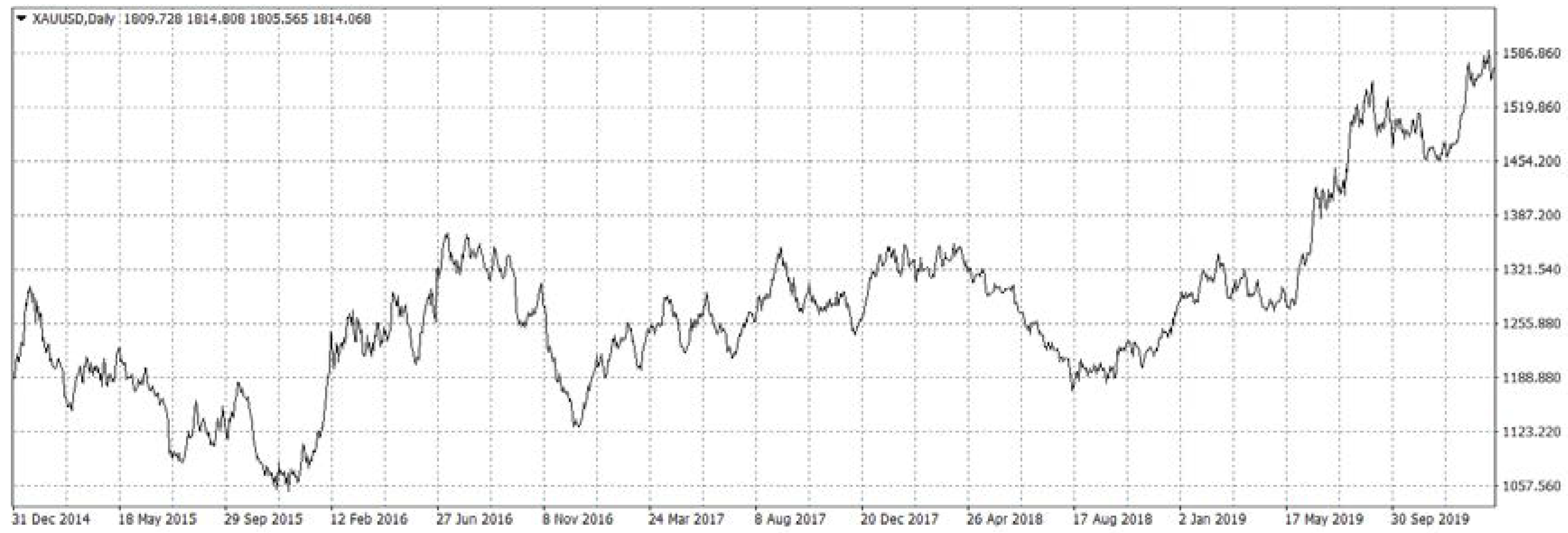
In this section, we explore the possibility of effective use of the CMUR system for speculations in exchange pair gold quoted in USD (XAU/USD). We have collected tick data containing 188,055,881 XAU/USD quotations from 31 December 2014 to 1 January 2020 [47]. For exchange pair XAU/USD, these tick data determine the Ask price trend. This trend graph is presented in Figure 2.

We see that the trend ${\mathrm{Q}}_{\mathrm{Ask}}$ contains descriptions of bull market, bear market rand, and sideways market. For this reason, we can say that the collected tick data are representative.

On 2 January 2020, the average price of 1 gold ounce was $1520.30. It means that average Ask price of 1 gold lot was $v_{XAU/USD}=\$152,030$. Trading on the XAU/USD exchange market is managed by many brokers. We assume that the speculator gives orders to a broker who offers a spread of $\overline{spr}=20 pips$. This level of spread is most often offered on the XAU/USD exchange market.

In our study, we evaluated all CMUR systems characterized by observation range $c=2,3,4,5$ and discretization unit $\delta =21,22,\dots ,2420$. It means that we examined the effectiveness of 9680 variants of the CMUR system. We will lead our statistical research at the significance level $\alpha =0.05$. The assumed research area results from our experience gathered during previous studies [24,25,26,27,28,29,30,31,32].

For each pair of control parameters $\left(\delta ,c\right),$ we determine following values and sets:

• ${ℰ}_{\delta ,c}$ the binary representation containing all binary observations (5),
• $n_{\delta ,c}$ the number of binary observations,
• ${\Psi }_{\delta ,c}$ the training dataset (10),
• $a_{\delta ,c}$ the average sample size given by the equation:

  $$a_{\delta ,c}=\frac{n_{\delta ,c}-c-1}{2^c},$$

  (57)
• $𝒫(XAG/USD,\delta ,c,{\Psi }_{\delta c)}$ the prediction table (16),
• $\mathbb{D}\left(0.05,\delta , c\right)$ the space of all well-justified premises (19),
• ${\mathbb{D}}_{\delta ,c}=\mathbb{D}\left(0.05,\delta , c,{\pi }_{𝓊p}\right)$ the space of all acceptable premises (24),
• ${\mathcal{N}}_{\delta ,c}$ the expected annual number of transactions (29),
• ${𝓎}_{\delta ,c}$ the expected unit payment (31),
• $i_{\delta ,c}$ the expected interest rate (33),
• ${ℰ}_{\delta ,c}$ the risk index (34).

A sample size will be applied for heuristic evaluation of obtained solutions of the optimization task.

In the next step, we use the algorithm (43–49) for each observation range, $c=2,3,4,5,$ separately. Obtained results are presented in

Table 5. Optimized variants of the CMUR system, $CMUR\left(𝒫\right(XAU/USD,\delta ,2,\Psi ),20,0.05)$

Discretization Unit $\delta$	Number of Binary Representations $n_{\delta ,2}$	Average Sample Size $a_{\delta ,2}$	Expected Interest Rate $i_{\delta ,2}$	Risk Index ${ℰ}_{\delta ,c}$
346	10,162	2540	36.10%	0.994099
528	4519	1129	38.58%	0.994164

Source: Own elaboration.

,

Table 6. Optimized variants of the CMUR system, $CMUR\left(𝒫\right(XAU/USD,\delta ,3,\Psi ),20,0.05)$.

Discretization Unit $\delta$	Number of Binary Representations $n_{\delta ,3}$	Average Sample Size $a_{\delta ,3}$	Expected Interest Rate $i_{\delta ,3}$	Risk Index ${ℰ}_{\delta ,3}$
375	8580	1072	55.90%	0.991297
376	8489	1061	59.37%	0.993476
463	5713	714	38.19%	0.985322

Source: Own elaboration.

,

Table 7. Optimized variants of the CMUR system, $CMUR\left(𝒫\right(XAU/USD,\delta ,4,\Psi ),20,0.05)$.

Discretization Unit $\delta$	Number of Binary Representations $n_{\delta ,4}$	Average Sample Size $a_{\delta ,4}$	Expected Interest Rate $i_{\delta ,4}$	Risk Index ${ℰ}_{\delta ,4}$
368	9021	564	55.02%	0.987849
375	8580	534	63.43%	0.990001
377	8498	531	66.08%	0.991844
404	7469	467	55.24%	0.988295
406	7385	461	38.28%	0.987462
418	6952	434	27.81%	0.979963
463	5713	357	51.54%	0.987502

Source: Own elaboration.

and

Table 8. Optimized variants of the CMUR system, $CMUR\left(𝒫\right(XAU/USD,\delta ,5,\Psi ),20,0.05)$.

Discretization Unit $\delta$	Number of Binary Representations $n_{\delta ,5}$	Average Sample Size $i_{\delta ,5}$	Expected Interest Rate $i_{\delta ,5}$	Risk Index ${ℰ}_{\delta ,5}$
366	9047	283	89.91%	0.985164
406	7385	231	83.19%	0.978913
442	6268	196	88.70%	0.98096
513	4740	148	37.54%	0.952324
515	4734	148	29.28%	0.920517
517	4702	147	56.99%	0.95236
537	4252	133	66.33%	0.96346
540	4218	132	79.09%	0.967076

Source: Own elaboration.

.

It is very easy to see that if we use the optimal CMUR system linked to observation range $c=5,$ then expected interest rates, $i_{\delta ,5},$ are not realistic. On the other hand, each average sample size, $i_{\delta ,5},$ is always low. Therefore, we can suppose that prediction tables $𝒫(XAU/USD,\delta ,5,\Psi )$ are not reliable. For this reason, we propose to accept the value $a=300$ as the minimal average sample size. Of course, our proposal is only heuristic. The above heuristic inference leads to the omission of the optimal CMUR systems, $CMUR\left(𝒫\right(XAU/USD,\delta ,5,\Psi ),20,0.05)$ in subsequent calculations.

In the last step, we use the algorithm (50–56) for all observation ranges, $c=2, 3, 4,$ together. Obtained results are presented in

Table 9. Effective variants of the CMUR system, $CMUR\left(𝒫\right(XAU/USD,\delta ,c,\Psi ),20,0.05)$.

Discretization Unit $\delta$ Unit Return Modulus	Observation Range $c$	Expected Annual Number of Transactions ${\mathcal{N}}_{\delta ,c}$	Expected Unit Payment ${𝓎}_{\delta ,c}$	Expected Interest Rate $i_{\delta ,c}$	Risk Index ${ℰ}_{\delta ,c}$
368	4	310.4	$269.49	63.43%	0.990001
375	4	406.6	$237.16	66.08%	0.991844
377	4	515.6	$194.84	55.24%	0.988295
404	4	279	$301.02	38.28%	0.987462
406	4	180	$323.29	27.81%	0.979963
418	4	85.4	$495.04	51.54%	0.987502
463	3	126.4	$459.34	38.19%	0.985322
463	4	196.2	$399.40	51.54%	0.987502

Source: Own elaboration.

.

The above table can be used as follows: A speculator chooses one of the recommended values of unit return modulus. This choice implies a recommendation of the proper observation range. An interesting situation exists in the case of a recommendation unit return modulus $\delta =463$. Then, we have two options of choice:

• The observation range $c=3$ for speculators with risk aversion.
• The observation range $c=4$ for speculators with risk propensity.

This is a simple example of the CMUR system flexibility.

7. Conclusions

In this paper, we proposed an original method of selecting financially effective CMUR systems. Proper selection is given as Pareto’ optimum determined by interest rate maximization and risk index minimization. In our case study, we show a heuristic limitation of optimization task. The results of the discussion point to further research directions.

Results obtained in the case study show that distinguished Pareto’s optima are multi-element sets. This fact implies that a most-powerful parameter specification does not exist. This is a common situation in economics and finance. For this reason, in economics and finance, we are finding non-dominated parameter specification. It is a widely accepted approach in operations research. Therefore, such approach is applied in our paper.

Moreover, obtained results show that distinguished Pareto’s optima are not convex. It implies that expected interest rate and risk index are not convex functions of CMUR system parameters. It implies that convex analysis cannot be used.

In our paper, we have used risk index (34) related to Shannon’ entropy [46]. It would be useful to discuss the use of other suitable risk indices here. We propose to discuss the following ex-ante risk indices: inverse of success probability (28), single payment variance, and single payment semi-variance. In addition, we suggest taking max drawdown into account as ex-post risk indices. A rank correlation between these indices should be investigated. After this research, we will be able to start comparing CMUR systems and other types of trading systems. In the case study, we proposed to accept some values as minimal average sample size. This proposal is only heuristic. This means that there is a real need to build a formal method of determining minimal sample size. Additionally, we propose the following directions of investigation on the CMUR systems:

• Influence of levering on CMUR system effectiveness, and
• Influence of lot value variability on systemic risk.

References

- Kaldor, N. Essays on Economic Stability and Growth; The Free Press of Glencoe Published by Gerald Duckworth: Glencoe, IL, USA, 1960. [Google Scholar]
- Huang, B.; Huan, Y.; Xu, L.D.; Zheng, L.; Zou, Z. Automated trading systems statistical and machine learning methods and hardware implementation: A survey. Enterp. Inf. Syst. 2019, 13, 132–144. [Google Scholar] [CrossRef]
- Dymova, L.; Sevastjanov, P.; Kaczmarek, K. A Forex trading expert system based on a new approach to the rule-base evidential reasoning. Expert Syst. Appl. 2016, 51, 1–13. [Google Scholar] [CrossRef]
- Piasecki, K.; Stasiak, M.D. The Forex Trading System for Speculation with Constant Magnitude of Unit Return. Mathematics 2019, 7, 623. [Google Scholar] [CrossRef] [Green Version]
- Komunikat w Sprawie Wyników Osiąganych Przez Inwestorów na Rynku Forex. Available online: https://www.knf.gov.pl/poprzednie_lata/komunikaty?articleId=53122&p_id=18 (accessed on 2 January 2019).
- News Releases AMF. 2014. Available online: https://www.amf-france.org/en_US/Actualites/Communiques-de-presse/AMF/annee_2014.html?docId=workspace%3A%2F%2FSpacesStore%2F96c52a14-3900-464f-8fff-7d4700ff37e3 (accessed on 2 January 2019).
- Aldridge, I. High-Frequency Trading: A Practical Guide to Algorithmic Strategies and Trading Systems, 2nd ed.; John Wiley and Sons: New York, NY, USA, 2013. [Google Scholar]
- Petropoulos, A.; Chatzis, S.P.; Siakoulis, V.; Vlachogiannakis, N. A stacked generalization system for automated FOREX portfolio trading. Expert Syst. Appl. 2017, 90, 290–302. [Google Scholar] [CrossRef]
- Bekiros, S.D. Heuristic learning in intraday trading under uncertainty. J. Empir. Financ. 2015, 30, 34–49. [Google Scholar] [CrossRef]
- Dunis, C.; Zhou, B. Nonlinear Modelling of High Frequency Financial Time Series; John Wiley & Sons: New York, NY, USA, 1998. [Google Scholar]
- Dempster, M.A.; Leemans, V. An automated FX trading system using adaptive reinforcement learning. Expert Syst. Appl. 2006, 30, 543–552. [Google Scholar] [CrossRef]
- Rundo, F.; Trenta, F.; Di Stallo, A.L.; Battiato, S. Advanced Markov-Based Machine Learning Framework for Making Adaptive Trading System. Computation 2019, 7, 4. [Google Scholar] [CrossRef] [Green Version]
- Dempster, M.A.; Jones, C.M. A real-time adaptive trading system using genetic programming. Quant. Financ. 2001, 1, 397–413. [Google Scholar] [CrossRef] [Green Version]
- Mendes, L.; Godinho, P.; Dias, J. A Forex trading system based on a genetic algorithm. J. Heuristics 2012, 18, 627–656. [Google Scholar] [CrossRef]
- Evans, C.; Pappas, K.; Xhafa, F. Utilizing artificial neural networks and genetic algorithms to build an algo-trading model for intra-day foreign exchange speculation. Math. Comput. Model. 2013, 58, 1249–1266. [Google Scholar] [CrossRef]
- Fischer, T.; Krauss, C. Deep learning with long short-term memory networks for financial market predictions. Eur. J. Oper. Res. 2018, 270, 654–669. [Google Scholar] [CrossRef] [Green Version]
- Li, Y.; Zheng, W.; Zheng, Z. Deep robust reinforcement learning for practical algorithmic trading. IEEE Access 2019, 7, 108014–108022. [Google Scholar] [CrossRef]
- Dixon, M.; Klabjan, D.; Bang, J.H. Classification-based financial markets prediction using deep neural networks. Algorithmic Financ. 2017, 6, 67–77. [Google Scholar] [CrossRef] [Green Version]
- Sezer, O.B.; Ozbayoglu, A.M. Algorithmic financial trading with deep convolutional neural networks: Time series to image conversion approach. Appl. Soft Comput. 2018, 70, 525–538. [Google Scholar] [CrossRef]
- Rundo, F.; Trenta, F.; di Stallo, A.L.; Battiato, S. Grid trading system robot (GTSbot): A novel mathematical algorithm for trading FX market. Appl. Sci. 2019, 9, 1796. [Google Scholar] [CrossRef] [Green Version]
- Alonso-Monsalve, S.; Suárez-Cetrulo, A.L.; Cervantes, A.; Quintana, D. Convolution on neural networks for high-frequency trend prediction of cryptocurrency exchange rates using technical indicators. Expert Syst. Appl. 2020, 149, 113250. [Google Scholar] [CrossRef]
- Barbosa, R.P.; Belo, O. Multi-agent forex trading system. In Agent and Multi-Agent Technology for Internet and Enterprise Systems; Hakansson, A., Hartung, R., Nguyen, N.T., Eds.; Springer: Berlin/Heidelberg, Germany, 2010; pp. 91–118. [Google Scholar]
- Aloud, M.; Fasli, M.; Tsang, E.; Dupuis, A.; Olsen, R. Modeling the High-Frequency FX Market: An Agent-Based Approach. Comput. Intell. 2017, 33, 771–825. [Google Scholar] [CrossRef]
- Stasiak, M.D. Modelling of Currency Exchange Rates Using a Binary Representation. In Information Systems Architecture and Technology, Proceedings of the 37th International Conference on Information Systems Architecture and Technology—ISAT 2016, Karpacz, Poland, 18–20 September 2016; Wilimowska, Z., Borzemski, L., Grzech, A., Świątek, J., Eds.; Advances in Intelligent Systems and Computing; Springer: Berlin, Germany, 2016; Volume 524, pp. 153–161. [Google Scholar] [CrossRef]
- Stasiak, M.D. Wave relations of exchange rates in binary-temporal representation. In Proceedings of the 35th International Conference Mathematical Methods in Economics MME 2017, Hradec Králové, Czech Republic, 13–15 September 2017; Prazak, P., Ed.; Gaudeamus, University of Hradec Kralove: Hradec Králové, Czech Republic, 2017; pp. 720–725. [Google Scholar]
- Stasiak, M.D. Modelling of Currency Exchange Rates Using a Binary-Wave Representation. In Proceedings of 38th International Conference on Information Systems Architecture and Technology—ISAT 2017. Part III, Szklarska Poręba, Poland, 17–19 September 2017; Wilimowska, Z., Borzemski, L., Grzech, A., Świątek, J., Eds.; Springer: Berlin/Heidelberg, Germany, 2017; pp. 27–37. [Google Scholar] [CrossRef]
- Stasiak, M.D. Modelling of Currency Exchange Rates Using a Binary-Temporal Representation. In Contemporary Trends in Accounting, Finance and Financial Institutions, Proceedings of the International Conference on Accounting, Finance and Financial Institutions (ICAFFI), Poznan, Poland, 19–21 October 2016; Choudhry, T., Mizerka, J., Eds.; Springer: Berlin/Heidelberg, Germany, 2018; pp. 97–110. [Google Scholar]
- Stasiak, M.D. A study on the influence of the discretisation unit on the effectiveness of modelling currency exchange rates using the binary-temporal representation. Oper. Res. Dec. 2018, 28, 57–70. [Google Scholar]
- Piasecki, K.; Stasiak, M. Exchange rate modelling with use of relative binary representation. In Proceedings of the 36th International Conference Mathematical Methods in Economics, Jindrichuv Hradec, Czech Republic, 12–14 September 2018; MatfyzPress, Publishing House of the Faculty of Mathematics and Physics Charles University: Prague, Czech Republic, 2018; pp. 410–415. [Google Scholar]
- Piasecki, K.; Stasiak, M.; Staszak, Ż. Investment Decision Support on Precious Metal Market with Use of Binary Representation, Effective Investments on Capital Markets. In Proceedings of the 10th Capital Market Effective Investments Conference (CMEI 2018), Międzyzdroje, Poland, 19 September 2018; Tarczyński, W., Nermend, K., Eds.; Springer Proceedings in Business and Economics; Springer International Publishing AG: Cham, Switzerland, 2019; pp. 423–438. ISBN 978-3-030-21273-5. [Google Scholar] [CrossRef]
- Stasiak, M. Trend analysis with use of binary representation. In Proceedings of the 37th International Conference Mathematical Methods in Economics MME 2019: Conference Proceedings, České Budějovice, Czech Republic, 11–13 September 2019; Houda, M., Remeš, R., Eds.; University of South Bohemia in České Budějovice, Faculty of Economics: České Budějovice, Czech Republic, 2019; pp. 529–535. ISBN 978-80-7394-760-6. [Google Scholar]
- Piasecki, K.; Stasiak, M. Verification of the Precious Metals Market Effectiveness—Gold and Silver. In Proceedings of the International Scientific Conference Hradec Economic Days, Hradec Králové, Czech Republic, 2–3 April 2020; Jedlička, P., Marešová, P., Firlej, K., Soukal, I., Eds.; University of Hradec Králové: Hradec Králové, Czech, 2020; Volume 10, pp. 1–9. [Google Scholar] [CrossRef]
- Chante, S. Beyond Technical Analysis: How to Develop and Implement a Winning Trading System; John Wiley & Sons: New York, NY, USA, 1997. [Google Scholar]
- Vastone, B.; Finnie, G. An empirical methodology for developing stock market trading systems using artificial neural networks. Expert Syst. Appl. 2009, 36, 6668–6680. [Google Scholar] [CrossRef] [Green Version]
- Nelson, D.M.; Pereira, A.C.; De Oliveira, R.A. Stock market’s price movement prediction with LSTM neural networks. In Proceedings of the International Joint Conference on Neural Networks, Anchorage, AK, USA, 14–19 May 2017; pp. 1419–1426. [Google Scholar]
- Chong, E.; Han, C.; Park, F.C. Deep learning networks for stock market analysis and prediction: Methodology, data representations, and case studies. Expert Syst. Appl. 2017, 83, 187–205. [Google Scholar] [CrossRef] [Green Version]
- Borovkova, S.; Tsiamas, I. An Ensemble of LSTM Neural Networks or High-Frequency Stock Market Classification. Quant. Financ. 2019, 38, 600–619. [Google Scholar] [CrossRef] [Green Version]
- Nakano, M.; Takahashi, A.; Takahashi, S. Bitcoin technical trading with artificial neural network. Phys. A Stat. Mech. Appl. 2018, 510, 587–609. [Google Scholar] [CrossRef]
- Shintate, T.; Pichl, L. Trend Prediction Classification for High Frequency Bitcoin Time Series with Deep Learning. J. Risk Financ. Manag. 2019, 12, 17. [Google Scholar] [CrossRef] [Green Version]
- De Villiers, V. The Point and Figure Method of Anticipating Stock Price Movements: Complete Theory and Practice; Stock Market Publications: New York, NY, USA, 1935. [Google Scholar]
- Geisser, S. Predictive Inference; Chapman and Hall: New York, NY, USA, 1993. [Google Scholar]
- Wallis, S.A. Binomial confidence intervals and contingency tests: Mathematical fundamentals and the evaluation of alternative methods. J. Quant. Linguist. 2013, 20, 178–208. [Google Scholar] [CrossRef] [Green Version]
- Brown, L.D.; Cai, T.T.; Das Gupta, A. Interval Estimation for a Binomial Proportion. Stat. Sci. 2001, 16, 101–133. [Google Scholar] [CrossRef]
- García, B.Q.; Gaytán, J.C.T.; Wolfskill, L.A. The Role of Technical Analysis in the Foreign Exchange Market. Glob. J. Bus. Res. 2012, 6, 17–22. [Google Scholar]
- Li, W.; Wong, M.C.; Cenev, J. High frequency analysis of macro news releases on the foreign exchange market: A survey of literature. Big Data Res. 2015, 2, 33–48. [Google Scholar] [CrossRef]
- Shannon, C.E. A Mathematical Theory of Communication. Bell Syst. Tech. J. 1948, 27, 379–423. [Google Scholar] [CrossRef] [Green Version]
- Gold Reaches 6-Month Maximum. Available online: https://fbs.eu/analytics/news/gold-reaches-6-month-maximum-4133 (accessed on 2 January 2019).
Figure 1.
The graph for trend of Ask price of XAG/USD exchange pair.
Figure 2.
The graph for trend of Ask price of XAU/USD exchange pair.