Article

Progressive Type-II Censoring Schemes of Extended Odd Weibull Exponential Distribution with Applications in Medicine and Engineering

1
Department of Mathematics and Statistics, College of Science, King Faisal University P.O. Box 400, Al-Ahsa 31982, Saudi Arabia
2
Department of Statistics, Faculty of Commerce Mansoura University, El-Mansoura 35516, Egypt
3
Department of Statistics, Faculty of Business Administration, Delta University of Science and Technology, El-Mansoura 11152, Egypt
4
Department of Statistics, Mathematics and Insurance, Benha University, Benha 13511, Egypt
*
Author to whom correspondence should be addressed.
Submission received: 26 August 2020 / Revised: 16 September 2020 / Accepted: 25 September 2020 / Published: 1 October 2020
(This article belongs to the Special Issue Probability, Statistics and Their Applications)

Abstract

:
In this paper, the parameters of the extended odd Weibull exponential distribution are estimated under progressive type-II censoring scheme with random removal. The model parameters are estimated using the maximum product spacing and maximum likelihood estimation methods. Further, we explore the asymptotic confidence intervals and bootstrap confidence intervals for the model parameters. Monte Carlo simulations are performed to compare between the proposed estimation methods under progressive type-II censoring scheme. An empirical study using two real datasets form engineering and medicine fields to validate the introduced methods of inference. Based on our study, we can conclude that the maximum product of spacing method outperforms the maximum likelihood method for estimating the extended odd Weibull exponential (EOWE) parameters under a progressive type-II censoring scheme in both numerical and empirical cases.

1. Introduction

Life-testing and reliability experiments contain many situations where units are removed or lost from the test before failure. For example, units may break accidently in an industrial experiment, individuals may drop out of the study in a clinical trial, or they have to be terminated early due to lack of funds. In many scenarios, the removal of units before failure is very often procedure due to limitations of time and cost associated with the experiment. The data of such tests or experiments are called censored data.
There are different types of censoring schemes which include right, left, interval censoring, single or multiple censoring and type-I or type-II censoring, but the conventional type-I and type-II censoring schemes do not have flexibility of allowing removal of units at point other than the terminal point of the experiment. A mixture of type-I and type-II schemes is known as the hybrid censoring scheme, which was first introduced by Epstein [1]. For this reason, we consider here a more general censoring scheme called progressive type-II censoring scheme. The progressively hybrid censoring scheme, has its favorable position, to be extremely mainstream in the reliability and life-testing over the last few years, which was introduced by Kundu and Joarder [2]. Furthermore, the progressive type-II censoring scheme includes the complete sample situation (if R i = 0 , i = 1 , 2 , , m with n = m ) and the conventional type-II right censoring scheme (if R i = 0 , i = 1 , 2 , , m 1 with R m = n m ) as special cases.
More details about progressive type-II censoring scheme can be explored in Balakrishnan and Aggarwala [3], Alshenawy R. [4], Balakrishnan [5] and Almetwally et al. [6].
In this paper, we extend the work of Afify and Mohamed [7] by considering the estimation of the extended odd Weibull exponential (EOWE) parameters under progressive type-II censoring scheme with random removal based on the maximum product spacing (MPS) and maximum likelihood estimation methods. Further, the interval estimation of the EOWE parameters are obtained using asymptotic and bootstrap confidence intervals based on progressive type-II censoring scheme. The performance of the proposed estimators is evaluated via extensive simulations. Applications of two real datasets are introduced to confirm the validity of the model.
The EOWE distribution is introduced by Afify and Mohamed [
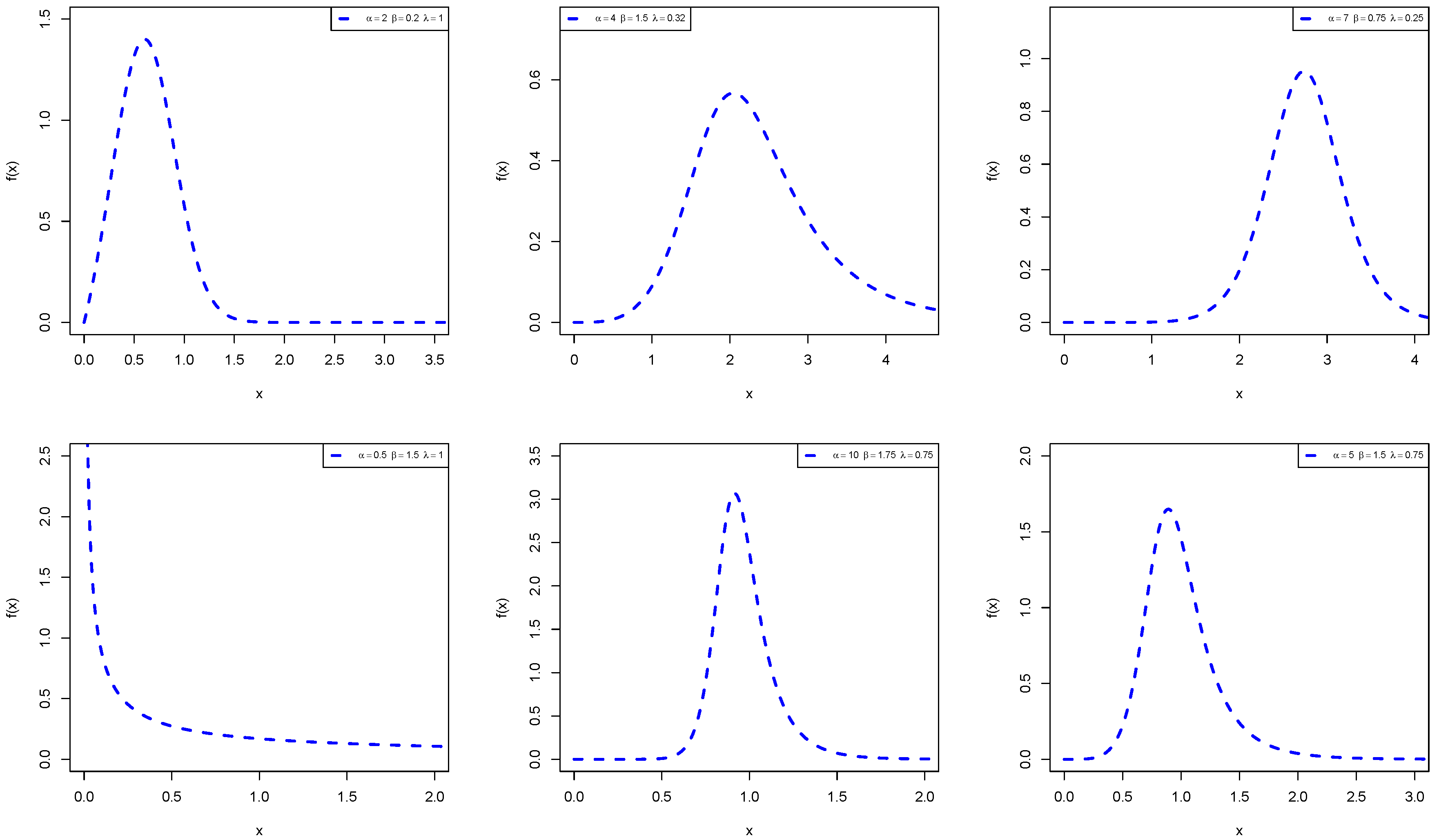
7] for modeling data in several fields such as engineering, medicine, and reliability. The EOWE distribution is a flexible model which provides left-skewed, symmetrical, right-skewed, and reversed-J shaped densities (See 
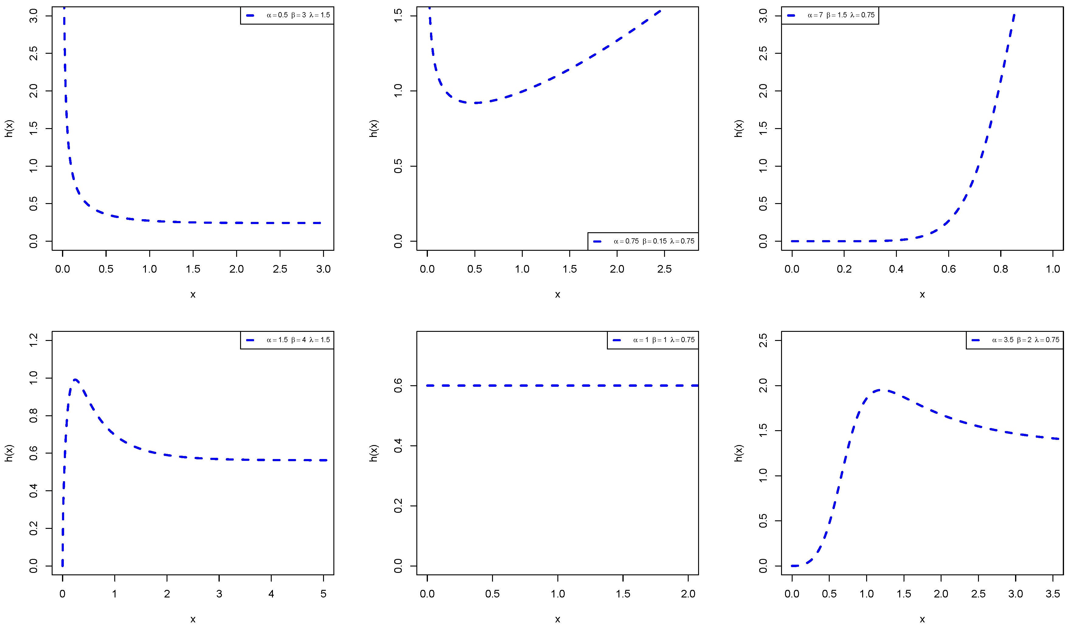
Figure 1). Its hazard rate function (HRF) can provide decreasing, constant, increasing, upside-down bathtub, bathtub, and reversed-J shaped hazard rates (See Figure 2). It is noted that, the bathtub and modified bathtub hazard rates are very important in the reliability engineering context. The interesting point of the EOWE distribution, with three parameters, is that it exhibits the bathtub and modified bathtub hazard rates as, in general, most distributions used to model such data are complicated, and usually may include four or five parameters to obtain these hazard rates. Due to its flexibility and simple closed forms of its HRF and cumulative distribution function (CDF), we can use it for analyzing censored data.
They also studied the estimation of its parameters using eight classical estimation methods called, the maximum product of spacing estimators, maximum likelihood estimators, least squares estimators, weighted least-squares estimators, percentiles estimators, Cramér-von Mises estimators, Anderson-Darling estimators, and right-tail Anderson-Darling estimators. They compared the performance of these estimators, for small and large samples, using extensive simulations.
The CDF and probability density function (PDF) of the EOWE distribution are given by
F ( x ; α , β , λ ) = 1 1 + β exp λ x 1 α 1 β , x > 0 , α , β , λ > 0
and
f ( x ; α , β , λ ) = α λ exp α λ x 1 exp λ x α 1 1 + β exp λ x 1 α 1 β 1 , x > 0 , α , β , λ > 0 ,
respectively. Henceforth, a random variable with PDF (2) is denoted by X EOWE ( α , β , λ ). The EOWE model reduces to the two-parameter Weibull exponential distribution for β 0 + .
The MPS method was presented by Cheng and Amin [8] and autonomously talked about by Ranneby [9] as an alternative method to the maximum likelihood estimation method for continuous distributions, for example see Almetwally and Almongy [10]. Ng et al. [11] discussed progressive type-II censored samples using the MPS method. Almetwally and Almongy [12] and Basu et al. [13] introduced the MPS method based on hybrid censoring scheme. Almetwally et al. [14,15] introduced the adaptive type-II progressive censoring schemes using MPS method. El-Sherpieny et al. [16] introduced progressive type-II hybrid censoring scheme based on MPS.
The rest of this paper is organized as follows. The model description is presented in Section 2. Parameter estimation are given in Section 3. We provide bootstrap confidence intervals in Section 4. In Section 5, the potentiality of the estimation approaches is assessed via simulation results. In Section 6, two applications to real data are discussed. Finally, some remarks are offered in Section 7.

2. Model Description and Formulation

The following assumptions will be employed under progressive type-II censoring scheme and can be described as follows.
  • Assume that n identical and independent units are put on a life test and the lifetimes of these units have the EOWE distribution.
  • Generate progressive sample as x 1 : m : n < x 2 : m : n < < x m : m : n , where m is prefixed where m n .
  • At first failure, R 1 of the surviving units n 1 are randomly removed from the test. After observing the second failure, R 2 of the surviving units n R 1 1 are randomly removed from the experiment. The process continues until the mth, denoted by R m , failure is occurred. After the mth failure the remaining surviving units R m = n m i = 1 m 1 R i are removed from the test and the experiment is terminated.
  • Suppose that an individual unit being removed from the test is independent of the others but with the same removal probability p. Then, the number of units removed at each failure time follows a binomial distribution. That is R i b i n o m i a l ( n m i = 1 m 1 R i , p ) .
The joint likelihood function based on progressive type-II censored sample with binomial removals is defined, for any vector of parameters Φ , as
l ( x i : m : n , Φ ) = L ( x i : m : n , Φ ) P ( R = r ) ,
where L ( x i : m : n , Φ ) is the likelihood function under progressive type II censored samples and
P ( R = r ) = ( n m ) ! ( n m j = 1 m 1 r j ) ! j = 1 m 1 r j p j = 1 m 1 r j ( 1 p ) ( m 1 ) ( n m ) j = 1 m 1 ( m j ) r j .
The maximum likelihood estimator (MLE) of p follows directly by maximizing P ( R = r ) in (4), since L ( x i : m : n , Φ ) does not depend on the binomial parameter p. Hence, the MLE of p follows as
p ^ = j = 1 m 1 r j ( m 1 ) ( n m ) j = 1 m 1 ( m j ) r j ) ! j = 1 m 1 r j .
Similarly, P ( R = r ) does not involve the parameter vector Φ , then the MLE of Φ can be obtained easily by maximizing L ( x i : m : n , Φ ) . More information can be explored in Tse et al. [17].
The likelihood function under progressive type-II censored samples is defined by (see Balakrishnan and Aggarwala [3])
L ( x i : m : n , Φ ) = C i = 1 m f ( x i : m : n , Φ ) 1 F ( x i : m : n , Φ ) R i ,
where C is a constant which does not depend on the parameters vector Φ and it is defined by C = n ( n R 1 1 ) ( n R 1 R 2 2 ) ( n m R 1 R m 1 + 1 ) .

3. Parameter Estimation under Progressive Type-II Censored Samples

In this section, we study the estimation problem of the EOWE parameters under progressive type-II censored samples using two estimation methods called, the maximum likelihood estimators (MLEs) and maximum product of spacing estimators (MPSEs).

3.1. Maximum Likelihood Method

Let X 1 : m : n , , X m : m : n be a progressively type-II censored sample from the EOWE distribution with with PDF (2) and parameters α , β , and λ . The log-likelihood function takes the form
= m log α + m log λ + α λ i = 1 m x i : m : n + α 1 i = 1 m log A i : m : n i = 1 m R i + β + 1 β log 1 + β K i : m : n α ,
where K i : m : n = e λ x i : m : n 1 , A i : m : n = 1 e λ x i : m : n . The MLEs of the parameters α , β and λ under progressive type-II censored samples, are obtained by differentiating the log-likelihood Equation (6) with respect to each parameter separately, by solving the following nonlinear equations,
α = m α + λ i = 1 m x i : m : n + i = 1 m log A i : m : n i = 1 m R i + 1 + β K i : m : n α log K i : m : n 1 + β K i : m : n α = 0 ,
β = i = 1 m R i + β + 1 β K i : m : n α 1 + β K i : m : n α + R i + 1 β 2 i = 1 m log 1 + β K i : m : n α = 0
and
λ = m λ + α i = 1 m x i : m : n + α 1 i = 1 m x i : m : n 1 A i : m : n A i : m : n α i = 1 m R i + β + 1 x i : m : n exp λ x i : m : n K i : m : n α 1 1 + β K i : m : n α = 0 .
These equations are very difficult to be solved, so nonlinear optimization algorithm as Newton–Raphson method are used. Using numerical analysis, the asymptotic confidence interval (ACI) can be obtained through asymptotic variance–covariance matrix and normal approximation confidence intervals.

3.2. Maximum Product Spacing Method

Cheng and Amin [8,18] introduced the MPS method as an alternative to MLE method for estimating the parameters of continuous univariate distributions. They replaced the likelihood function by product of spacings and stated that the MPS method possesses most of the maximum likelihood properties. Further, Ranneby [9] independently proposed the MPS method as an approximation to the Kullback-Leibler measure of information.
The consistency and asymptotic properties of the MPSEs are discussed in [8,18] and the authors also observed that the MPSEs are at least as efficient as the MLEs when they exit. Coolen and Newby [19] discussed the invariance property of MPSEs and stated that it is the same as that of the MLEs. Furthermore, the MPSEs are quite effective and many authors proposed the use of this method as a good alternative to the MLEs, and found that this estimation approach can provide better estimates than the maximum likelihood approach in several situations in both complete and censored samples. For more details, the reader may refer to Ghosh and Jammalamadaka [20], Rahman and Pearson [21], Singh et al. [22], Basu et al. [23], Almetwally and Almongy [12] Al-Mofleh et al. [24], Sen [25].
Consider a progressively type-II censored sample, say X 1 : m : n , , X m : m : n , from the EOWE distribution with with PDF (2) and parameters α , β , and λ . Then, the uniform spacings of this random sample are defined as
D i x i : m : n ; α , β , λ = F x 1 : m : n ; α , β , λ if i = 1 , F x i : m : n ; α , β , λ F x i 1 : m : n ; α , β , λ if i = 2 , , m , 1 F x m : m : n ; α , β , λ if i = m ,
The MPSEs can be obtained by maximizing the product of spacings which are defined under progressive type-II censoring sample as follows (see Ng et al. [11])
P S ( x i : m : n ; α , β , λ ) = C i = 1 m D ( x i : m : n , α , β , λ ) 1 F ( x i : m : n , α , β , λ ) R i ,
where C is a constant term and it does not depend on parameters α , β and λ .
Using the CDF of the EOWE distribution and the logarithm of product of spacings, we obtain
S ( x i : m : n ; α , β , λ ) = log 1 1 + β K 1 : m : n α 1 β + 1 β log 1 + β K 1 : m : n α + i = 2 m log 1 + β K 1 : m : n α 1 + β K 1 : m : n α + i = 1 m R i β log 1 + β K 1 : m : n α ,
where K i : m : n = e λ x i : m : n 1 .
The MPSEs of α , β , and λ under progressively type-II censored samples are obtained by solving the following nonlinear equations, which are follows by differentiating the logarithm of product of spacings in Equation (7) with respect to each parameter
S ( x i : m : n ; α , β , λ ) α = ( 1 : m : n ) 1 β β δ 1 : m : n 1 ( 1 : m : n ) 1 β + δ m : m : n m : m : n + β i = 2 m log δ i 1 : m : n δ i : m : n i 1 : m : n i : m : n + i = 1 m R i β δ i : m : n i : m : n = 0 ,
S ( x i : m : n ; α , β , λ ) β = 1 : m : n 1 β log ( 1 : m : n ) K 1 : m : n α β 2 ( 1 1 : m : n 1 β ) 1 β 2 log m : m : n + 1 β K m : m : n α m : m : n + i = 2 m K i 1 : m : n α K i : m : n α i 1 : m : n i : m : n i = 1 m R i β 2 log i : m : n + i = 1 m R i β K i : m : n α i : m : n = 0
and
S ( x i : m : n ; α , β , λ ) λ = 1 β 1 : m : n 1 β 1 φ 1 : m : n 1 1 : m : n 1 β + 1 β φ m : m : n m : m : n + i = 2 m φ i 1 : m : n φ i : m : n i 1 : m : n i : m : n + i = 1 m R i β φ i : m : n i : m : n = 0 ,
where δ i : m : n = K i : m : n α log ( K i : m : n ) , i : m : n = 1 + β K 1 : m : n α , and φ i : m : n = β α K i : m : n α 1 e λ x i : m : n x i : m : n .
These equations are very difficult to be solved analytically, hence the nonlinear optimization algorithms such as Newton–Raphson method can be employed to solve these equations numerically. Using numerical analysis, the ACI follows by asymptotic variance–covariance matrix and normal approximation confidence intervals.

4. Bootstrap Confidence Intervals

In this section, we propose different bootstrap confidence intervals. We adopt the percentile bootstrap (Bp) confidence intervals and bootstrap-t (Bt) confidence intervals. More information about bootstrap confidence intervals can be found in Efron [26], Hall [27], and El-Morshedy et al. [28].

4.1. Percentile Bootstrap Confidence Intervals

The following steps illustrate how to calculate the Bp confidence interval for the EOWE parameters.
  • Compute the MLEs of the parameters α , β and λ .
  • Generate a bootstrap samples using α , β and λ to obtain the bootstrap estimates, α b , β b and λ b using the bootstrap samples.
  • Repeat step (2) B times to have ( α b ( 1 ) , α b ( 2 ) , , α b ( B ) ) , ( β b ( 1 ) , β b ( 2 ) , , β b ( B ) ) and ( λ b ( 1 ) , λ b ( 2 ) , λ b ( B ) ) .
  • Arrange ( α b ( 1 ) , α b ( 2 ) , , α b ( B ) ) , ( β b ( 1 ) , β b ( 2 ) , , β b ( B ) ) and ( λ b ( 1 ) , λ b ( 2 ) , λ b ( B ) ) in ascending order as ( α b [ 1 ] , α b [ 2 ] , , α b ( [ B ] ) ) , ( β b [ 1 ] , β b [ 2 ] , , β b ( [ B ] ) ) and ( λ b [ 1 ] , λ b [ 2 ] , λ b [ B ] ) .
  • The two sided 100 ( 1 γ ) % Bp confidence intervals for the unknown parameters α , β and λ are given by [ α b ( [ B γ 2 ] ) , α b ( [ B ( 1 γ 2 ) ] ) ] , [ β b ( [ B γ 2 ] ) , β b ( [ B ( 1 γ 2 ) ] ) ] and [ λ b ( [ B γ 2 ] ) , λ b ( [ B ( 1 γ 2 ) ] ) ] .

4.2. Bootstrap-t Confidence Intervals

The Bt confidence intervals for the EOWE parameters can be calculated using the following steps.
  • Applying the same first two steps (1 and 2) as in Bp.
  • Compute the t-statistic of Φ as T = Φ ^ b Φ ^ V ( Φ ^ b ) where V ( Φ ^ b ) is asymptotic variances of Φ ^ b and it can be obtained using the Fisher information matrix, where Φ = ( α , β , λ ) T .
  • Repeat the step (2) B times to obtain ( T ( 1 ) , T ( 2 ) , , T ( B ) ) .
  • Arrange ( T ( 1 ) , T ( 2 ) , , T ( B ) ) in ascending order as ( T [ 1 ] , T [ 2 ] , , T [ B ] ) .
  • The two sided 100 ( 1 γ ) % Bt confidence intervals for the unknown parameters α , β and λ are defined by [ α + T k b ( [ B γ 2 ] ) V ( α b ) , β + V ( α b ) T k b ( [ B ( 1 γ 2 ) ] ) ] , [ β + T k b ( [ B γ 2 ] ) V ( β b ) ,   β + V ( β b ) T k b ( [ B ( 1 γ 2 ) ] ) ] and [ λ + T k b ( [ B γ 2 ] ) V ( λ b ) , λ + V ( λ b ) T k b ( [ B ( 1 γ 2 ) ] ) ] .

5. Simulation Study

In this section, Monte-Carlo simulations are conducted to compare between the MLEs and MPSEs, of the EOWE parameters, under progressive type-II censored samples with binomial removals, using the R software. The simulation results are conducted to explore and assess the properties and performance of the MLEs and MPSEs in terms of their biases, mean square error (MSEs), and length of confidence interval (L.CI). We generate 10,000 random samples from the EOWE distribution for the following parameter combinations.
Case I:
α = 3.5 , β = 3 and λ = 0.5 ,
Case II:
α = 3.5 , β = 1.5 and λ = 0.5 and
Case III:
α = 3.5 , β = 1.5 and λ = 1.5
For different sample sizes n = 50 , 100 and 200, different number of failures m and removal probabilities p = 0.25 and p = 0.75 to generate the number of units removed at each failure time R i using the binomial distribution. It is supposed that an individual unit being removed from the test is independent of the others but with the same removal probabilities p = 0.25 and p = 0.75 . Then, the number of units removed at each failure time follows the binomial distribution.
The confidence level for confidence intervals (CIs) is 95% where, γ is 0.05. The estimation method which minimizes the biases, MSEs, and L.CI of the estimates can be considered the best scheme. Table 1, Table 2 and Table 3 summarize the simulation results including the bias, MSEs, L.CI, Bp, and Bt for the MLEs and MPSEs for different parameter combinations.
From Table 1, Table 2 and Table 3, the following observations can be summarized as follows.
  • The MSEs, bias and L.CI decrease as the sample size increases for all parameter combinations.
  • The bias, MSEs, L.CI decrease as the number of stages (m) increases.
  • The MPS estimates are efficient than the maximum likelihood (ML) estimates for most studied cases of the EOWE distribution under progressive type-II censored samples with binomial removals.
  • The MSEs of MPSEs are smaller than the MSEs of MLEs, hence the MPS method outperforms the ML method under progressive type-II censoring scheme.
  • The length of confidence intervals of the MPS approach are comes out to be smaller than those of the ML approach for most considered cases.
  • The Bt confidence intervals are more efficient than the Bp confidence intervals for most studied cases.
From the values in Table 1, Table 2 and Table 3, we can conclude that the MPS method outperforms the ML method in estimating the parameters of the EOWE distribution under progressive type-II censoring scheme with binomial removals.

6. Applications to Real Data

We present the numerical results of estimating the parameters of EOWE model under progressive type-II censoring scheme using two real datasets from the engineering and medicine fields, to illustrate the methods of inference discussed in Section 3.
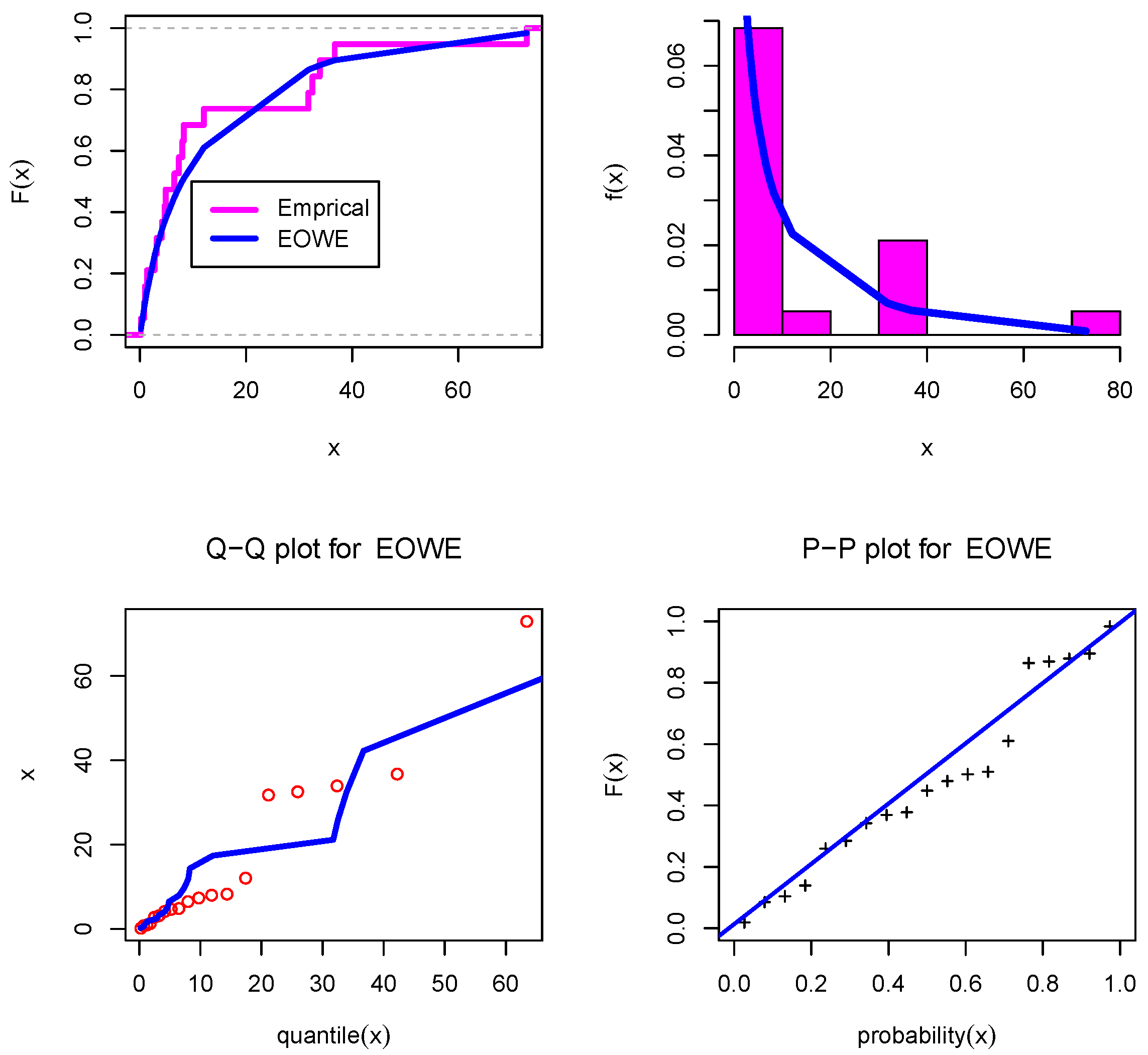
The first data refer to electric data (Balakrishnan and Cramer [29]). Theses data contain 19 measurements of failure times (in minutes) for an insulating fluid between two electrodes subject to a voltage of 34 kV: 0.19, 0.78, 0.96, 1.31, 2.78, 3.16, 4.15, 4.67, 4.85, 6.50, 7.35, 8.01, 8.27, 12.06, 31.75, 32.52, 33.91, 36.71 and 72.89. We computed the Kolmogorov-Smirnov (KS) distance (D) between the fitted and the empirical distribution functions for the data, where KS = 0.17449 and its corresponding p-value = 0.5515. Figure 3 displays the plots of estimated CDF, fitted PDF, PP-plot and QQ-plot for the EOWE distribution for complete data. Figure 3 indicates that the EOWE distribution provides better fits to electric data.
Table 4 shows the parameter estimates, their standard errors (SEs), lower and upper CI (L.CI and U.CI) for the EOWE distribution using the MPS and ML methods. These data are progressive type-II censored data with censoring scheme R = ( 0 ( 2 ) , 3 , 0 , 3 , 0 ( 2 ) , 5 ) . The censored data are listed in Table 5. We also computed the KS of ML method distance is 0.26316 and its corresponding p-value is 0.1192. Table 6 shows ML and MPS estimates, SEs, L.CI and U.CI under progressive censored electric data.
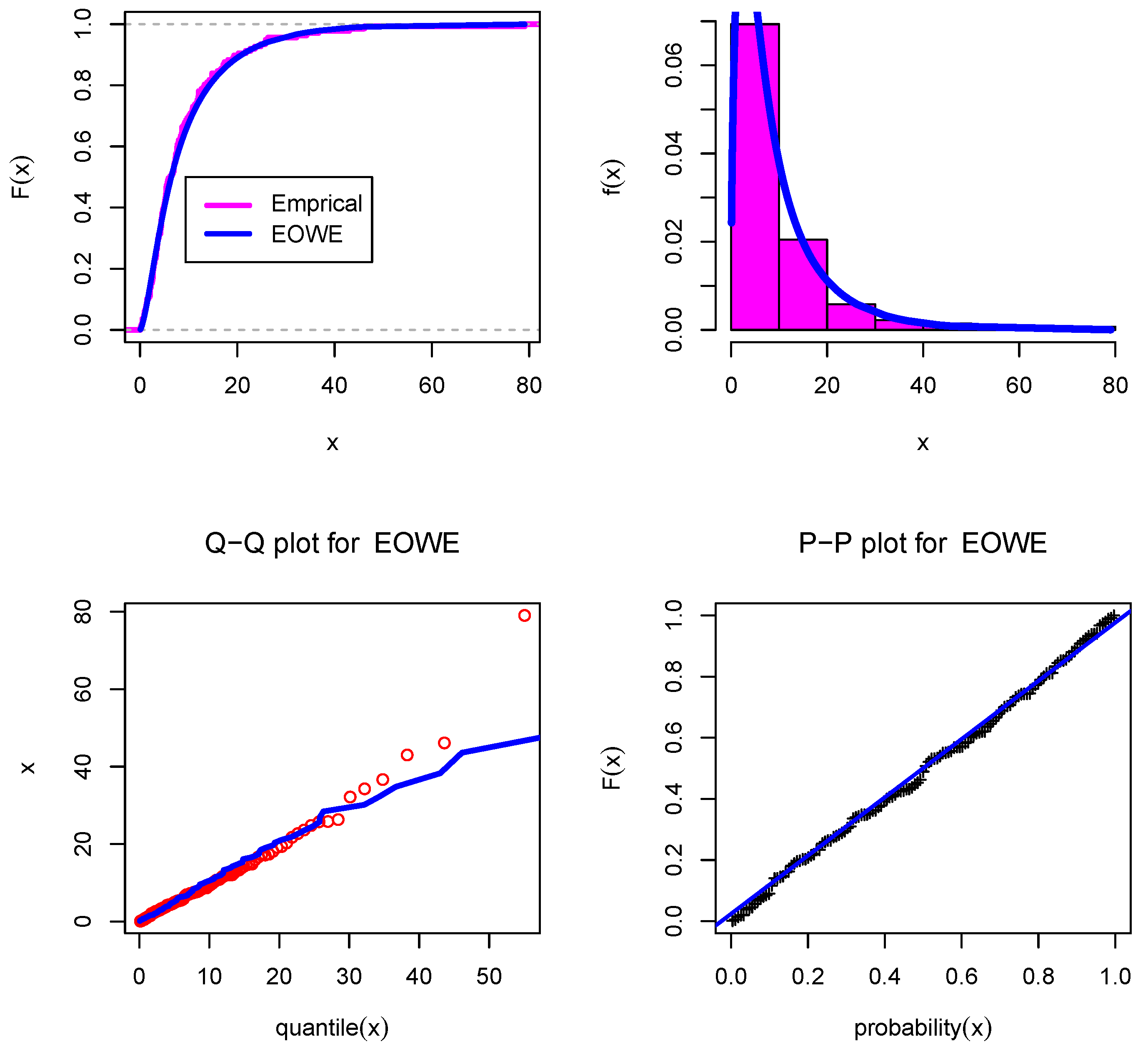
The second dataset is discussed by Lee and Wang [30], and it represents the remission times (in months) of a random sample of 137 bladder cancer patients. Figure 4 shows the plots of the estimated CDF, fitted PDF, PP-plot and QQ-plot for the EOWE distribution. This figure indicates that the EOWE distribution can provide better fit to the medicine data. Table 7 shows ML and modified MPS estimates, SEs, L.CI, U.CI, KS test for complete medicine data.
These data are progressive type-II censored data with censoring scheme R = ( 0 ( 2 ) , 3 , 0 , 3 , 0 ( 2 ) , 5 ) . The four randomly generated censored samples based on bladder cancer data are reported in Appendix A. We also computed the KS of ML method distance is 0.26316 and its corresponding p-value is 0.1192. Table 8 reports the parameter estimates, their SEs, L.CI and U.CI for the EOWE distribution using ML and modified MPS methods. Table 8 reveals that the length of confidence intervals of the modified MPS approach are smaller than those of the ML method. Based on the values in Table 8, we can conclude that the modified MPS method outperforms the ML method in estimating the EOWE parameters under progressive type-II censored bladder cancer data for different removal probabilities p = 0.25 and p = 0.75 .

7. Conclusions

In this article, the maximum product spacing and maximum likelihood estimation methods are adopted for estimating the parameters of the EOWE distribution under progressive type-II censoring scheme with binomial removals. The performance of the two proposed estimators is investigated numerically for different parameter values and sample sizes using simulations. The percentile bootstrap and bootstrap-t confidence intervals are determined for the proposed estimation methods. Moreover, the roles of sample size n, failure size m, and removal probabilities p toward the accuracy of estimates are studied via simulation results. Based on our study, we can conclude that the maximum product of spacing method provides better performance than the maximum likelihood estimation method in estimating the EOWE parameters under progressive type-II censored samples. Finally, two real data examples, from engineering and medicine fields, are explored to illustrate the methods of inference discussed in the paper. Finally, based on our study, we can confirm the superiority of the maximum product of spacing method for estimating the EOWE parameters form the two real datasets under progressive type-II censoring scheme.

Author Contributions

R.A., A.A.-A., E.M.A., A.Z.A. and H.M.A. contributed equally to this work. All authors have read and agreed to the published version of the manuscript.

Funding

This research received no external funding.

Acknowledgments

The authors would like to thank the Editorial Board, and two referees for their constructive remarks and suggestions which greatly improved the final version of this manuscript.

Conflicts of Interest

The authors declare no conflict of interest.

Appendix A

Case I: The sample observations under progressive type-II censoring schemes for bladder cancer data with m = 100 , p = 0.25 and R = ( 8 , 11 , 1 , 6 , 3 , 0 , 3 , 1 , 2 , 1 , 0 ( 3 ) , 1 , 0 ( 86 ) ) :
0.20 0.40 0.87 1.26 1.35 1.46 1.76 2.02 2.02 2.07 2.09 2.23 2.46 2.54 2.62 2.64 2.75 2.83 2.87 3.02 3.25 3.31 3.36 3.36 3.48 3.64 3.70 3.82 3.88 4.18 4.23 4.26 4.33 4.33 4.34 4.40 4.50 4.51 4.65 4.70 4.87 5.17 5.32 5.34 5.41 5.41 5.49 5.62 5.71 5.85 6.54 6.76 6.93 6.94 6.97 7.09 7.39 7.59 7.62 7.63 7.66 7.87 8.53 8.60 8.65 8.66 9.02 9.74 10.34 10.66 10.86 11.25 11.64 11.79 12.02 12.03 12.07 12.63 13.11 13.80 14.24 14.76 14.77 14.83 15.96 17.36 18.10 19.13 20.28 23.63 24.80 25.74 25.82 26.31 32.15 34.26 36.66 43.01 46.12 79.05.
Case II: The sample observations under progressive type-II censoring schemes for bladder cancer data with m = 100 , p = 0.75 and R = ( 7 , 19 , 11 , 0 ( 97 ) ) :
0.08 0.51 0.81 0.90 1.26 1.35 1.40 1.46 2.02 2.09 2.23 2.26 2.46 2.62 2.64 2.69 2.69 2.83 2.87 3.02 3.25 3.31 3.36 3.52 3.57 3.64 3.70 3.82 3.88 4.18 4.26 4.33 4.33 4.34 4.40 4.50 4.51 4.65 4.70 4.87 5.06 5.09 5.17 5.32 5.32 5.34 5.41 5.41 5.49 5.62 5.85 6.54 6.76 6.97 7.09 7.28 7.39 7.63 7.66 8.26 8.65 8.66 9.02 9.22 9.47 10.06 10.34 10.66 10.75 10.86 11.25 11.64 11.79 11.98 12.02 12.03 12.63 13.11 13.80 14.24 14.77 14.83 15.96 16.62 17.12 17.14 18.10 19.13 19.36 20.28 21.73 22.69 23.63 24.80 25.74 26.31 32.15 34.26 36.66 46.12.
Case III: The sample observations under progressive type-II censoring schemes for bladder cancer data with m = 120 , p = 0.25 and R = ( 4 , 5 , 0 , 3 , 1 , 0 , 2 , 0 , 1 , 0 ( 4 ) , 1 , 0 ( 106 ) ) :
0.20 0.51 0.87 0.90 1.19 1.26 1.35 1.40 1.46 2.02 2.02 2.07 2.09 2.23 2.26 2.46 2.54 2.62 2.64 2.69 2.75 2.83 2.87 3.02 3.02 3.25 3.31 3.36 3.36 3.48 3.52 3.57 3.64 3.82 3.88 4.18 4.23 4.33 4.40 4.50 4.51 4.65 4.70 4.87 4.98 5.06 5.17 5.32 5.32 5.34 5.41 5.41 5.49 5.62 5.71 5.85 6.25 6.54 6.76 6.93 6.94 6.97 7.09 7.26 7.28 7.32 7.39 7.62 7.63 7.66 7.87 7.93 8.26 8.37 8.53 8.60 8.65 8.66 9.02 9.22 9.47 9.74 10.06 10.66 10.75 10.86 11.64 11.79 11.98 12.02 12.07 12.63 13.11 13.29 13.80 14.24 14.76 14.77 14.83 15.96 16.62 17.14 17.36 18.10 19.13 19.36 20.28 21.73 22.69 23.63 24.80 25.74 25.82 26.31 32.15 34.26 36.66 43.01 46.12 79.05.
Case IV: The sample observations under progressive type-II censoring schemes for bladder cancer data with m = 120 , p = 0.75 and R = ( 3 , 10 , 3 , 1 , 0 ( 96 ) ) :
0.08 0.20 0.40 0.50 0.51 0.81 0.87 0.90 1.05 1.19 1.26 1.35 1.40 1.46 1.76 2.02 2.07 2.09 2.23 2.54 2.62 2.64 2.69 2.69 2.75 2.83 2.87 3.02 3.02 3.31 3.36 3.36 3.48 3.64 3.70 3.82 3.88 4.18 4.23 4.26 4.33 4.33 4.34 4.40 4.50 4.51 4.65 4.70 4.98 5.06 5.09 5.17 5.32 5.32 5.34 5.41 5.49 5.62 5.71 5.85 6.25 6.54 6.76 6.93 6.94 6.97 7.09 7.26 7.28 7.32 7.39 7.59 7.62 7.63 7.66 7.87 7.93 8.26 8.37 8.53 8.60 8.66 9.02 9.22 9.47 9.74 10.06 10.66 10.75 10.86 11.25 11.79 11.98 12.02 12.03 12.07 12.63 13.80 14.24 14.77 14.83 15.96 16.62 17.12 18.10 19.13 19.36 20.28 22.69 23.63 24.80 25.74 25.82 26.31 32.15 34.26 36.66 43.01 46.12 79.05.

References

  1. Epstein, B. Estimation from life test data. Technometrics 1960, 2, 447–454. [Google Scholar] [CrossRef]
  2. Kundu, D.; Joarder, A. Analysis of type-II progressively hybrid censored data. Comput. Stat. Data Anal. 2006, 50, 2509–2528. [Google Scholar] [CrossRef]
  3. Balakrishnan, N.; Aggrawalla, R. Progressive Censoring: Theory, Methods and Applications; Berkhauser: Boston, MA, USA, 2000. [Google Scholar]
  4. Alshenawy, R. A new one parameter distribution: Properties and estimation with applications to complete and type II censored data. J. Taibah Univ. Sci. 2020, 14, 11–18. [Google Scholar] [CrossRef] [Green Version]
  5. Balakrishnan, N. Progressive censoring methodology: An appraisal. Test 2007, 16, 211–259. [Google Scholar] [CrossRef]
  6. Almetwally, E.M.; Almongy, H.M.; Mubarak, A.E. Bayesian and maximum likelihood estimation for the Weibull generalized exponential distribution parameters using progressive censoring schemes. Pak. J. Stat. Oper. Res. 2018, 14, 853–868. [Google Scholar] [CrossRef]
  7. Afify, A.Z.; Mohamed, O.A. A new three-parameter exponential distribution with variable shapes for the hazard rate: Estimation and applications. Mathematics 2020, 8, 135. [Google Scholar] [CrossRef] [Green Version]
  8. Cheng, R.; Amin, N. Maximum Product of Spacings Estimation with Application to the Lognormal Distribution; Mathematical Report 79-1; University of Wales: Cardiff, UK, 1979. [Google Scholar]
  9. Ranneby, B. The maximum spacing method. An estimation method related to the maximum likelihood method. Scand. J. Stat. 1984, 11, 93–112. [Google Scholar]
  10. Almetwally, E.M.; Almongy, H.M. Estimation Methods for the new Weibull-Pareto distribution: Simulation and application. J. Data Sci. 2019, 17, 610–630. [Google Scholar]
  11. Ng, H.K.T.; Luo, L.; Hu, Y.; Duan, F. Parameter estimation of three-parameter Weibull distribution based on progressively type-II censored samples. J. Stat. Comput. Simul. 2012, 82, 1661–1678. [Google Scholar] [CrossRef]
  12. Almetwally, E.M.; Almongy, H.M. Maximum product spacing and Bayesian method for parameter etimation for generalized power Weibull distribution under censoring scheme. J. Data Sci. 2019, 17, 407–444. [Google Scholar]
  13. Basu, S.; Singh, S.K.; Singh, U. Estimation of inverse Lindley distribution using product of spacings function for hybrid censored data. Methodol. Comput. Appl. Probab. 2019, 21, 1377–1394. [Google Scholar] [CrossRef]
  14. Almetwally, E.M.; Almongy, H.M.; ElSherpieny, E.A. Adaptive type-II progressive censoring schemes based on maximum product spacing with application of generalized Rayleigh distribution. J. Data Sci. 2019, 17, 802–831. [Google Scholar]
  15. Almetwally, E.M.; Almongy, H.M.; Rastogi, M.K.; Ibrahim, M. Maximum product spacing estimation of Weibull distribution under adaptive type-II progressive censoring schemes. Ann. Data Sci. 2020, 7, 257–279. [Google Scholar] [CrossRef]
  16. El-Sherpieny, E.S.A.; Almetwally, E.M.; Muhammed, H.Z. Progressive type-II hybrid censored schemes based on maximum product spacing with application to power Lomax distribution. Physica A 2020, 553, 124251. [Google Scholar] [CrossRef]
  17. Tse, S.K.; Yang, C.; Yuen, H.K. Statistical analysis of Weibull distributed lifetime data under type II progressive censoring with binomial removals. J. Appl. Stat. 2020, 27, 1033–1043. [Google Scholar] [CrossRef]
  18. Cheng, R.; Amin, N. Estimating parameters in continuous univariate distributions with a shifted origin. J. R. Stat. Soc. Ser. B Methodol. 1983, 45, 394–403. [Google Scholar] [CrossRef]
  19. Coolen, F.P.A.; Newby, M.J. A Note on the Use of the Product of Spacings in Bayesian Inference; Memorandum COSOR; Technische Universiteit Eindhoven: Eindhoven, The Netherlands, 1990; Volume 9035. [Google Scholar]
  20. Ghosh, K.; Jammalamadaka, S.R. A general estimation method using spacings. J. Stat. Plan. Infer. 2001, 93, 71–82. [Google Scholar] [CrossRef] [Green Version]
  21. Rahman, M.; Pearson, L.M. Estimation in two-parameter exponential distributions. J. Stat. Comput. Simul. 2001, 70, 371–386. [Google Scholar] [CrossRef]
  22. Singh, K.R.; Singh, S.K.; Singh, U. Maximum product spacings method for the estimation of parameters of generalized inverted exponential distribution under Progressive type II censoring. J. Stat. Manag. Syst. 2016, 19, 219–245. [Google Scholar]
  23. Basu, S.; Singh, S.K.; Singh, U. Bayesian inference using product of spacings function for progressive hybrid type-I censoring scheme. Statistics 2018, 52, 345–363. [Google Scholar] [CrossRef]
  24. Al-Mofleh, H.; Afify, A.Z.; Ibrahim, N.A. A new extended two-parameter distribution: Properties, estimation methods, and applications in medicine and geology. Mathematics 2020, 8, 1578. [Google Scholar] [CrossRef]
  25. Sen, S.; Afify, A.Z.; Al-Mofleh, H.; Ahsanullah, M. The quasi xgamma-geometric distribution with application in medicine. Filomat 2019, 33, 5291–5330. [Google Scholar] [CrossRef] [Green Version]
  26. Efron, B. The Jackknife, the Bootstrap and Other Resampling Plans; SIAM: Philadelphia, PA, USA, 1982. [Google Scholar]
  27. Hall, P. Theoretical comparison of bootstrap confidence intervals. Ann. Stat. 1988, 16, 927–953. [Google Scholar] [CrossRef]
  28. El-Morshedy, M.; Alhussain, Z.A.; Atta, D.; Almetwally, E.M.; Eliwa, M.S. Bivariate Burr X generator of distributions: Properties and estimation methods with applications to complete and type-II censored samples. Mathematics 2020, 8, 264. [Google Scholar] [CrossRef] [Green Version]
  29. Balakrishnan, N.; Cramer, E. The Art of Progressive Censoring: Applications to Reliability and Quality; Statistics for Industry and Technology; Springer: New York, NY, USA; Heidelberg, Germany; Dordrecht, The Netherlands; London, UK, 2014. [Google Scholar]
  30. Lee, E.T.; Wang, J. Statistical Methods for Survival Data Analysis; John Wiley Sons: Hoboken, NJ, USA, 2003; Volume 476. [Google Scholar]
Figure 1. Different possible shapes of the extended odd Weibull exponential (EOWE) density function for several parametric values.
Mathematics 08 01679 g001
Figure 2. Different possible shapes of the EOWE hazard function for several parametric values.
Mathematics 08 01679 g002
Figure 3. The estimated cumulative distribution function (CDF), fitted probability density function (PDF), PP-plot and QQ-plot of the EOWE distribution for complete electric data.
Mathematics 08 01679 g003
Figure 4. The estimated CDF, fitted PDF, PP-plot and QQ-plot of the EOWE distribution for complete bladder cancer data.
Mathematics 08 01679 g004
Table 1. The maximum likelihood estimators (MLEs) and maximum product of spacing estimators (MPSEs) of the EOWE parameters under progressive type-II censoring scheme with binomial removals for Case I.
MLEsMPSEs
n p m BiasMSEsL.CIBpBtBiasMSEsL.CIBpBt
500.2530 α 0.35230.65722.86350.08890.08880.04010.46312.97670.08250.0822
β 0.09320.93193.76850.11980.11580.09520.74753.30840.11040.1089
λ −0.03390.00410.21160.00660.0065−0.03570.00390.20300.00640.0064
45 α 0.19060.56242.84480.08630.0872−0.08600.37922.66810.07520.0759
β 0.03350.81283.53340.11060.11030.08190.64783.15150.10280.1060
λ 0.00040.00250.19780.00650.0065−0.00040.00230.19050.00570.0057
0.7530 α 0.46781.56104.54370.14870.14210.14070.71103.58770.10300.1027
β 0.17262.49766.16110.23600.19970.20621.14504.08440.13390.1356
λ −0.00960.00300.21220.00660.0067−0.01130.00280.20490.00670.0067
45 α 0.20860.62412.98830.09770.0979−0.07640.39822.74170.07900.0791
β 0.13321.00263.89210.12330.11820.11040.67233.20930.10310.1010
λ 0.00180.00250.19590.00630.00630.00090.00220.18690.00610.0062
1000.2560 α 0.30210.34661.98190.06070.06070.11910.28982.24220.06720.0668
β 0.08900.48042.69590.08720.08680.08510.45112.62730.08590.0829
λ −0.01530.00210.16770.00510.0051−0.01690.00190.16090.00500.0050
85 α 0.13160.19981.67550.04870.0491−0.02250.17671.80060.05010.0509
β 0.03820.34652.30390.07350.07490.03860.31482.19480.07100.0704
λ −0.00300.00120.13810.00430.0042−0.00410.00120.13680.00430.0042
0.7560 α 0.31430.58992.74840.08900.08860.10200.31522.37770.07010.0689
β 0.17941.07544.00590.12650.12780.16080.61433.02720.09330.0932
λ −0.00240.00240.19140.00610.0061−0.00480.00200.17820.00570.0055
85 α 0.10520.20701.73590.05430.0552−0.06360.17531.79170.05220.0519
β 0.05160.36782.37000.06880.06980.03030.30742.19250.06840.0681
λ −0.00010.00130.14240.00450.0045−0.00180.00130.14020.00470.0047
2000.25130 α 0.10280.06080.87890.02740.02770.01790.05190.97550.02800.0277
β −0.01250.04800.85830.02810.02810.01360.06180.94730.03020.0300
λ −0.00790.00070.09550.00320.0032−0.00820.00070.09690.00310.0030
180 α 0.04120.04560.82220.02570.0257−0.03240.03980.84580.02400.0237
β −0.00430.04570.83790.02600.02570.01210.04030.76940.02770.0277
λ −0.00170.00050.08500.00270.0028−0.00160.00050.08440.00270.0027
0.75130 α 0.08950.06000.89410.02890.0289−0.00110.05280.99210.02720.0271
β 0.01780.06450.99330.03120.03100.03630.06760.99100.03340.0320
λ −0.00290.00070.10380.00330.0033−0.00330.00070.10300.00330.0033
180 α 0.03550.06000.95020.02950.0298−0.03860.05290.96370.02820.0284
β 0.00880.05530.92150.02930.02940.02520.04770.83430.02830.0277
λ −0.00170.000470.08440.00270.0027−0.00170.000450.08320.00260.0026
Table 2. The MLEs and MPSEs of the EOWE parameters under progressive type-II censoring scheme with binomial removals for Case II.
MLEsMPSEs
n p m BiasMSEsL.CIBpBtBiasMSEsL.CIBpBt
500.2530 α 0.33370.55292.60600.08080.07990.10340.39872.67340.07860.0799
β −0.01200.48302.72530.08720.08700.10140.44102.46070.08090.0836
λ −0.02550.00270.17910.00580.0057−0.02360.00260.17390.00570.0056
45 α 0.12470.34532.25210.07220.0712−0.04900.31282.35870.07050.0702
β 0.01870.35232.32690.07690.07810.10370.36602.25260.07310.0732
λ −0.00060.00170.16010.00500.00510.00280.00160.15500.00480.0049
0.7530 α 0.41090.89263.33670.11640.11430.17420.51922.97860.08920.0883
β 0.10010.92213.74560.12070.11960.19380.54842.70950.09090.0889
λ −0.00590.00240.18970.00600.0062−0.00330.00210.17700.00580.0059
45 α 0.12380.34542.25310.07330.0733−0.06980.29392.30220.06770.0660
β 0.01790.28432.09000.06770.06630.08580.27861.97470.06160.0617
λ −0.00040.00150.15230.00490.00500.00230.00150.14930.00480.0049
1000.2560 α 0.18340.12711.19920.03790.03730.09290.13661.49360.04550.0461
β −0.00740.13171.42290.04470.04460.08540.16651.47220.05230.0500
λ −0.01210.00120.12570.00370.0037−0.00960.00120.12630.00400.0040
85 α 0.06500.06170.94050.02820.0285−0.02210.05491.00220.02940.0294
β −0.02570.04150.79300.02430.02410.03660.04950.79800.02780.0278
λ −0.00290.00060.09360.00280.0028−0.00060.00060.09310.00300.0030
0.7560 α 0.15550.16131.45250.04600.04610.05640.16321.66770.04970.0494
β 0.00840.16151.57570.04930.04890.09690.20061.62640.05460.0548
λ −0.00450.00120.13280.00420.0042−0.00170.00110.12960.00430.0044
85 α 0.03520.06440.98560.03080.0308−0.05400.06031.02900.02780.0284
β −0.02290.05130.88360.02840.02850.03580.04900.79820.02660.0260
λ −0.00170.00060.09620.00300.00300.00070.000600.09330.00310.0031
2000.25130 α 0.22600.24031.70630.05250.05250.14620.19041.69230.05010.0498
β 0.10210.18341.63120.05180.05190.13210.16241.46320.04710.0469
λ −0.00100.00060.09890.00320.0032−0.00020.00060.09340.00310.0031
180 α 0.04860.06680.99550.02990.0297−0.00520.06361.04230.03060.0305
β 0.00880.07251.05570.03400.03380.04010.07241.01210.03340.0334
λ −0.00080.000410.07960.00260.00260.00040.000400.07750.00240.0024
0.75130 α 0.18940.20441.61030.05080.05010.11420.17011.62940.04750.0474
β 0.10100.13891.40720.04120.04230.13690.13401.29540.04210.0412
λ 0.00190.00060.09410.00290.00300.00310.00050.08940.00290.0028
180 α 0.02730.05990.95370.02980.0303−0.02370.06751.06550.03280.0325
β 0.00000.06511.00090.03250.03250.03380.07231.01270.03310.0333
λ −0.00170.000370.07560.00250.0025−0.00040.000370.07490.00230.0023
Table 3. The MLEs and MPSEs of the EOWE parameters under progressive type-II censoring scheme with binomial removals for Case III.
MLEsMPSEs
n p m BiasMSEsL.CIBpBtBiasMSEsL.CIBpBt
500.2530 α 0.57361.52944.29700.13730.13700.28741.09774.23750.12900.1274
β 0.14740.98233.84390.11790.11900.24020.92163.55250.12120.1226
λ −0.06700.03110.64020.02060.0207−0.06270.02830.60810.02010.0199
45 α 0.28851.17264.09340.12520.12610.03730.72953.59790.10800.1087
β 0.13790.88483.64930.11460.11380.16940.71083.20770.10050.0995
λ 0.00250.02220.58370.01920.01910.00870.02040.55250.01680.0168
0.7530 α 0.65841.80584.59450.15240.15240.37791.24364.39540.13780.1386
β 0.26461.15924.09310.13510.13850.37051.23834.00950.12950.1289
λ −0.00520.02920.67010.02160.02160.00250.02700.63670.02070.0206
45 α 0.27971.15544.07030.13740.13660.03530.86893.89780.11840.1182
β 0.13660.87883.63730.12130.12050.17410.88153.58100.11260.1113
λ 0.00210.02200.58100.01860.01870.00850.02050.55350.01740.0176
1000.2560 α 0.54111.01453.33170.10190.10200.36900.75213.25020.09790.0996
β 0.25550.65753.01830.09700.09700.30500.62102.80030.09260.0930
λ −0.00960.01650.50220.01600.0160−0.00710.01520.48050.01470.0147
85 α 0.24740.54582.73030.08390.08630.10580.38582.54200.07370.0729
β 0.12240.41492.48020.07970.07930.14680.33912.18560.07530.0750
λ 0.00370.01040.40030.01280.01260.00670.00970.38250.01230.0121
0.7560 α 0.49111.06523.56020.11190.11140.31920.78943.42390.10660.1066
β 0.26960.75033.22830.10360.10450.31660.69162.96890.09510.0961
λ 0.01270.01730.51390.01640.01670.01670.01610.48890.01670.0165
85 α 0.17050.44522.52990.08170.08130.03870.36662.50150.07490.0777
β 0.08460.35072.29890.07340.07250.11610.32692.16420.07290.0719
λ 0.00260.01040.40060.01250.01260.00660.009800.38330.01270.0126
2000.25130 α 0.23840.24891.71900.05330.05380.16150.21021.75990.05530.0543
β 0.11070.19561.67960.05390.05470.14670.20281.63390.05360.0530
λ −0.00220.00620.30930.01000.00980.00070.00610.30280.01000.0100
180 α 0.07710.14201.44680.04340.04340.01130.12471.45030.04260.0431
β 0.02950.11561.32840.04140.04240.05130.11211.27600.04150.0417
λ −0.00080.00460.26510.00870.00830.00170.004420.25810.00780.0078
0.75130 α 0.21300.24161.73750.05590.05590.13530.20921.79150.05310.0531
β 0.12390.19461.66070.04960.05040.15970.20351.61870.05070.0502
λ 0.00780.00670.31910.00990.00980.01130.00660.31130.00990.0099
180 α 0.18420.22721.72430.05680.05600.10660.19471.75670.05480.0538
β 0.10540.18131.61800.05210.05300.13660.18521.56920.04960.0493
λ 0.00540.00610.30610.00950.00950.00850.005970.29790.00960.0096
Table 4. Estimates, standard errors (SEs), lower and upper CI (L.CI and U.CI) using the MLE and MPS methods for for complete electric data.
MLEsMPSEs
EstimatesSEsL.CIU.CIEstimatesSEsL.CIU.CI
α 1.14630.46290.23912.05360.87430.36080.16711.5815
β 3.72291.71860.35457.09142.66281.30590.10325.2224
λ 0.16820.07890.01350.32280.13230.06590.00320.2614
Table 5. Censored electric data generated under progressive type-II censoring scheme.
i12345678
R00303005
X i : m : n 0.190.780.961.312.74.856.57.35
Table 6. Estimates, SEs, L.CI, and U.CI using the MLE and MPS methods under progressive censored electric data.
MLEsMPSEs
EstimatesSEsL.CIU.CIEstimatesSEsL.CIU.CI
α 8.962515.84950.000040.02751.36369.07390.000019.1485
β 233.5237501.97250.00001217.390231.3125102.111631.1738431.4513
λ 2.78171.52200.00005.764816.58921.507213.635119.5433
Table 7. Estimates, SEs, L.CI, and U.CI using the ML and modified MPS methods for complete bladder cancer data.
MLEsMPSEs
EstimatesSEsL.CIU.CIEstimatesSEsL.CIU.CI
α 1.453620.0386221.377921.529321.393880.0333821.3284521.519048
β 1.9888230.402681.1995712.7780751.9585420.3658451.2414872.705878
λ 0.130890.0004360.1300360.1317450.1293320.0004180.1285130.13171
Table 8. Estimates, SEs, L.CI, and U.CI using the ML and modified MPS methods under progressive censored bladder cancer data.
MLEsMPSEs
p Estimates SEs L.CI U.CI Estimates SEs L.CI U.CI
1000.25 α 1.42750.04871.33211.52291.35750.03991.27931.4357
β 1.95570.58170.81563.09571.92200.50710.92822.9159
λ 0.12060.00060.11950.12170.11850.00050.11750.1196
0.75 α 1.47090.05001.37291.56901.39780.04141.31661.4790
β 1.99410.54480.92633.06191.96850.48421.01952.9176
λ 0.12980.00060.12860.13090.12790.00060.12680.1289
1200.25 α 1.80640.09701.61621.99661.72790.08131.56861.8872
β 2.55800.96730.66214.45392.48080.84210.83034.1314
λ 0.14010.00070.13880.14130.13770.00060.13660.1389
0.75 α 1.48420.04631.39341.57501.41110.03891.33481.4874
β 2.08830.49731.11363.06302.03350.44101.16912.8978
λ 0.12730.00050.12640.12820.12510.00040.12420.1260

