Article

Image Denoising Using Adaptive and Overlapped Average Filtering and Mixed-Pooling Attention Refinement Networks

1
Department of Electronics and Computer Engineering, National Taiwan University of Science and Technology, Taipei 10607, Taiwan
2
Department of Computer Science, National Chengchi University, Taipei 11605, Taiwan
*
Author to whom correspondence should be addressed.
Submission received: 16 March 2021 / Revised: 7 May 2021 / Accepted: 12 May 2021 / Published: 17 May 2021
(This article belongs to the Special Issue Artificial Intelligence and Big Data Computing)

Abstract

:
Cameras are essential parts of portable devices, such as smartphones and tablets. Most people have a smartphone and can take pictures anywhere and anytime to record their lives. However, these pictures captured by cameras may suffer from noise contamination, causing issues for subsequent image analysis, such as image recognition, object tracking, and classification of an object in the image. This paper develops an effective combinational denoising framework based on the proposed Adaptive and Overlapped Average Filtering (AOAF) and Mixed-pooling Attention Refinement Networks (MARNs). First, we apply AOAF to the noisy input image to obtain a preliminarily denoised result, where noisy pixels are removed and recovered. Next, MARNs take the preliminary result as the input and output a refined image where details and edges are better reconstructed. The experimental results demonstrate that our method performs favorably against state-of-the-art denoising methods.

1. Introduction

With the popularity of smartphones, the embedded cameras on phones have gradually replaced traditional digital cameras. However, when the light passes through the camera lens and is received by the image sensors, signals received through the analog to the digital circuit may be tampered with due to the surge voltage or high temperature of the sensors, resulting in signal errors and causing impulse noise. It severely degrades the visual quality of the images taken [1] and harms the accuracy of subsequent computer vision applications, such as object segmentation [2], detection, and tracking [3]. Therefore, it is critical to develop an effective method to remove image noise.
There are many image noise types, including impulse noise, Gaussian noise, and Poisson noise. Among the types of image noise, one of the most common impulse noises is salt-and-pepper (SP) noise. SP noise usually presents a small black dot or white dot with extreme intensities in the image. One of the most straightforward approaches to remove SP noise is to apply median filtering [4]. However, it introduces artifacts and blurriness to the denoised results since filtered pixels can be contaminated by noisy pixels. In addition, if median filtering uses a larger kernel, including irrelevant pixels in filtering, the results can be blurred. Hence, switching median filters [5,6,7] use multiple thresholds to switch among different filters. Nevertheless, determining appropriate thresholds is difficult and could affect the denoising performance.
Esakkirajan et al. [8] proposed the Modified Decision-Based Unsymmetrical Trimmed Median Filter (MDBUTMF) to use median or average filtering selectively. Still, it only works for low-density noisy images but often fails to deal with high-density noisy images. Erkan et al. developed the Different Applied Median Filter (DAMF)  [9], a two-pass median filter with three different mask sizes ( 3 × 3 , 5 × 5 , 7 × 7 ). Although filtering the input image containing high-level noise twice can generate better results, it may cause broken and fake edges in the image. Fareed et al. [10] presented an alternative method, called Fast Adaptive and Selective Mean Filter (FASMF), with a kernel whose size can grow from 3 × 3 to 7 × 7 based on the number of non-noise pixels around the noise ones, such as the DAMF. The FASMF averages non-noise pixels to replace noisy pixels. Using mean filtering could cause fewer fake edges but make the denoised result more blurred. Piyush Satti et al. [11] proposed a multi-procedure Min–Max Average Pooling-based filter (MMAP) to remove SP noise. However, it does not do well for images with high-density noise due to its small kernel size ( 3 × 3 ).
Other than pure filtering, image denoising using variational methods [12,13,14] is quite common. However, these learning-based methods could fail when dealing with high-density noisy images since the learned mapping from a few noise-free pixels to the entire image is ill-posed and thus does not work well.
Deep learning has achieved great success in many image processing tasks. It has also been applied to image denoising. Ulyanov et al. proposed Deep Image Prior [15] based on self-supervised learning to use a deep autoencoder for removing image noise. Xing et al. [16] proposed to remove SP noise from images using multiple denoisers based on convolutional neural networks (CNN), each of which is for a different noise level. Laine et al. [17] presented a high-quality deep image denoising method for Gaussian or impulse noise. However, deep-learning-based denoising models often fail to handle images with high-density noise directly.
This paper proposes a combinational denoising framework that can restore images with high-density noise. The framework includes Adaptive and Overlapped Average Filtering (AOAF) and Mixed-pooling Attention Refinement Networks (MARNs). The proposed AOAF adopts average filtering with adaptive kernel size and smooths noisy pixels in an overlapped manner to produce a preliminarily denoised result. The MARNs can refine the preliminary result to reconstruct details and edges. Combining AOAF and MARNs, we can effectively clean high-density noise and restore image texture and details. The primary contributions of this work are two-fold:
  • We propose a combinational filtering framework that can successfully remove high-density SP noise. The source code is made public here: https://github.com/Sasebalballgit/-Image-Denoising-using-AOAF-and-MARNs (accessed on 12 May 2021) for academic purposes only.
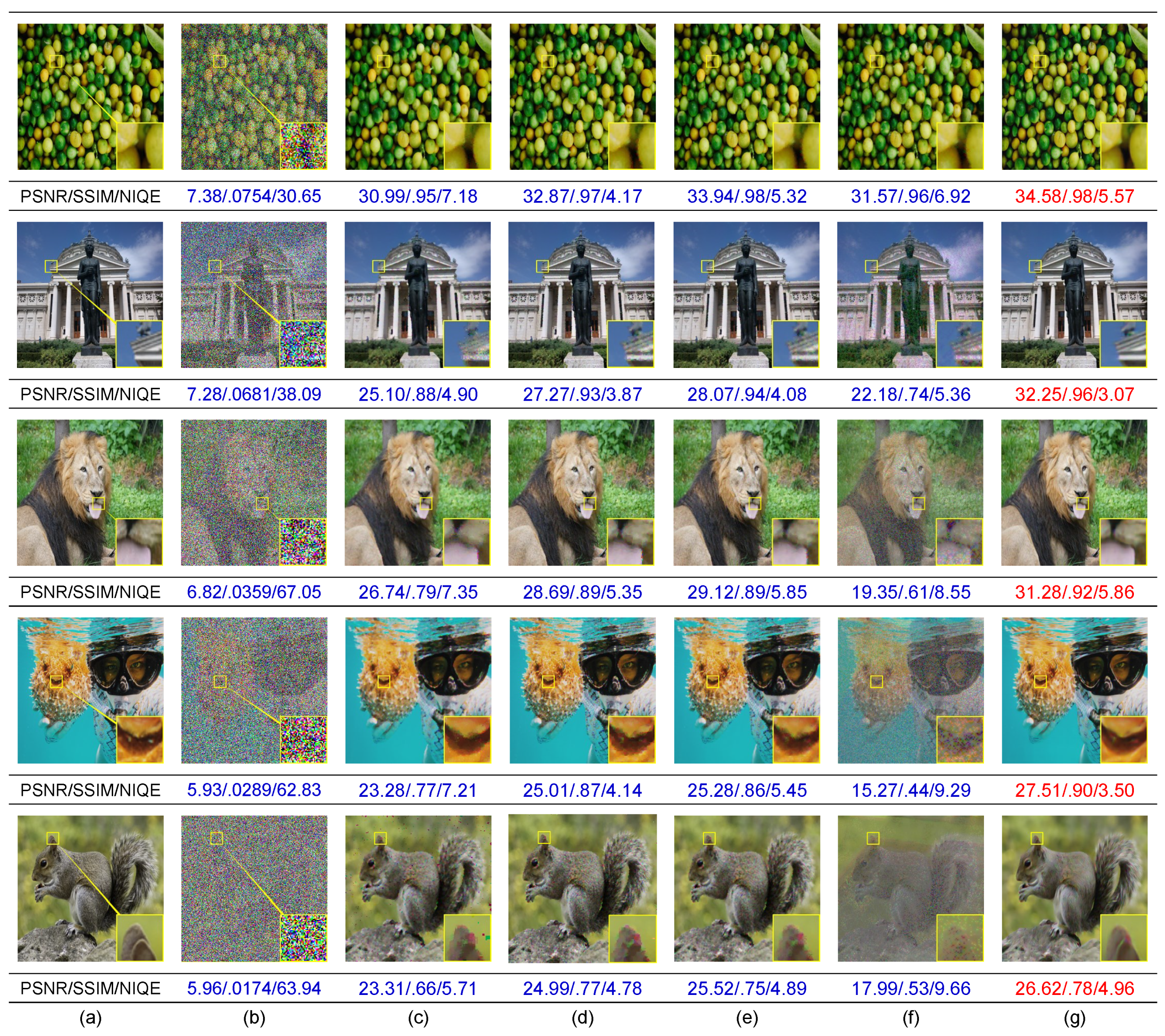
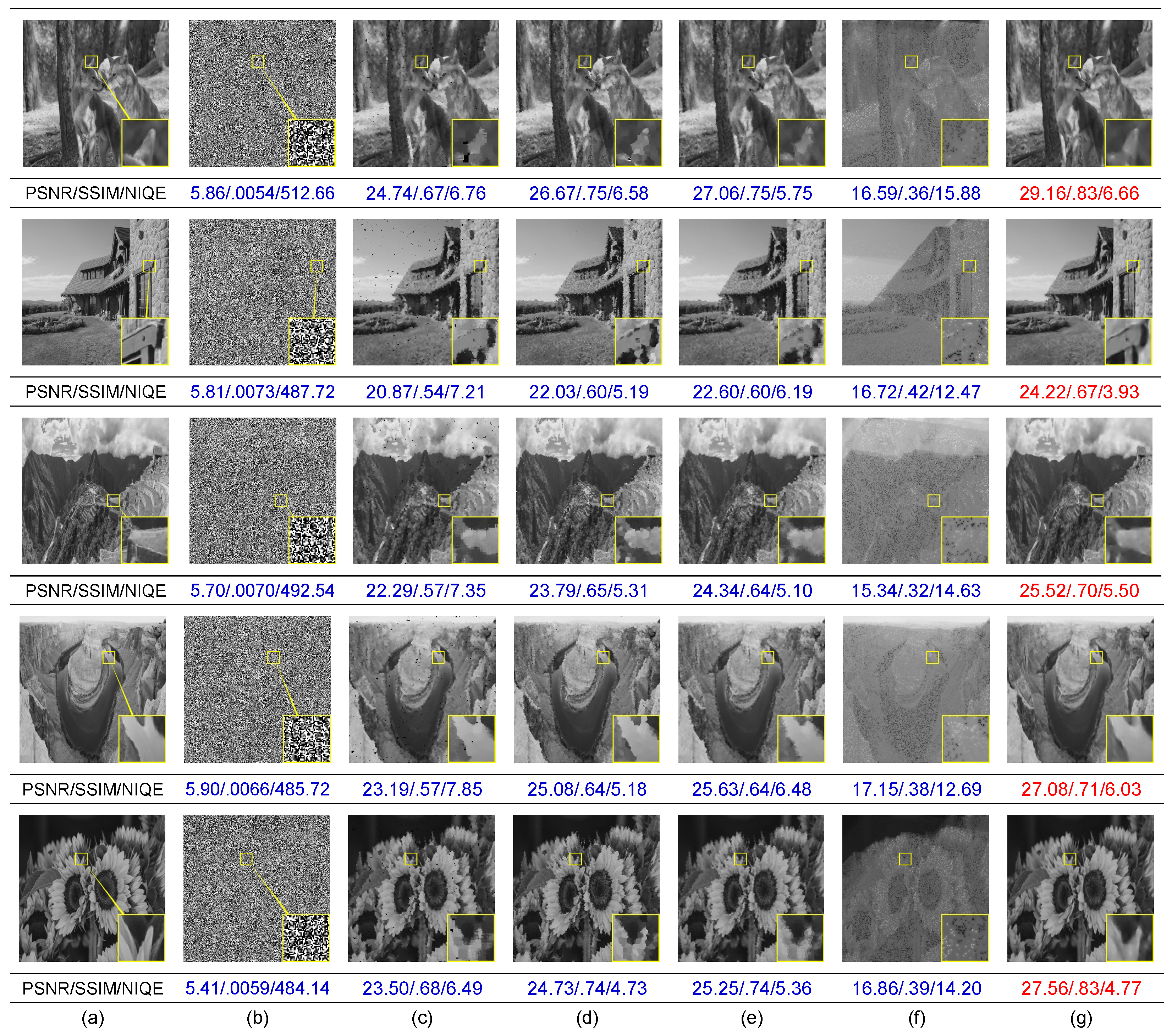
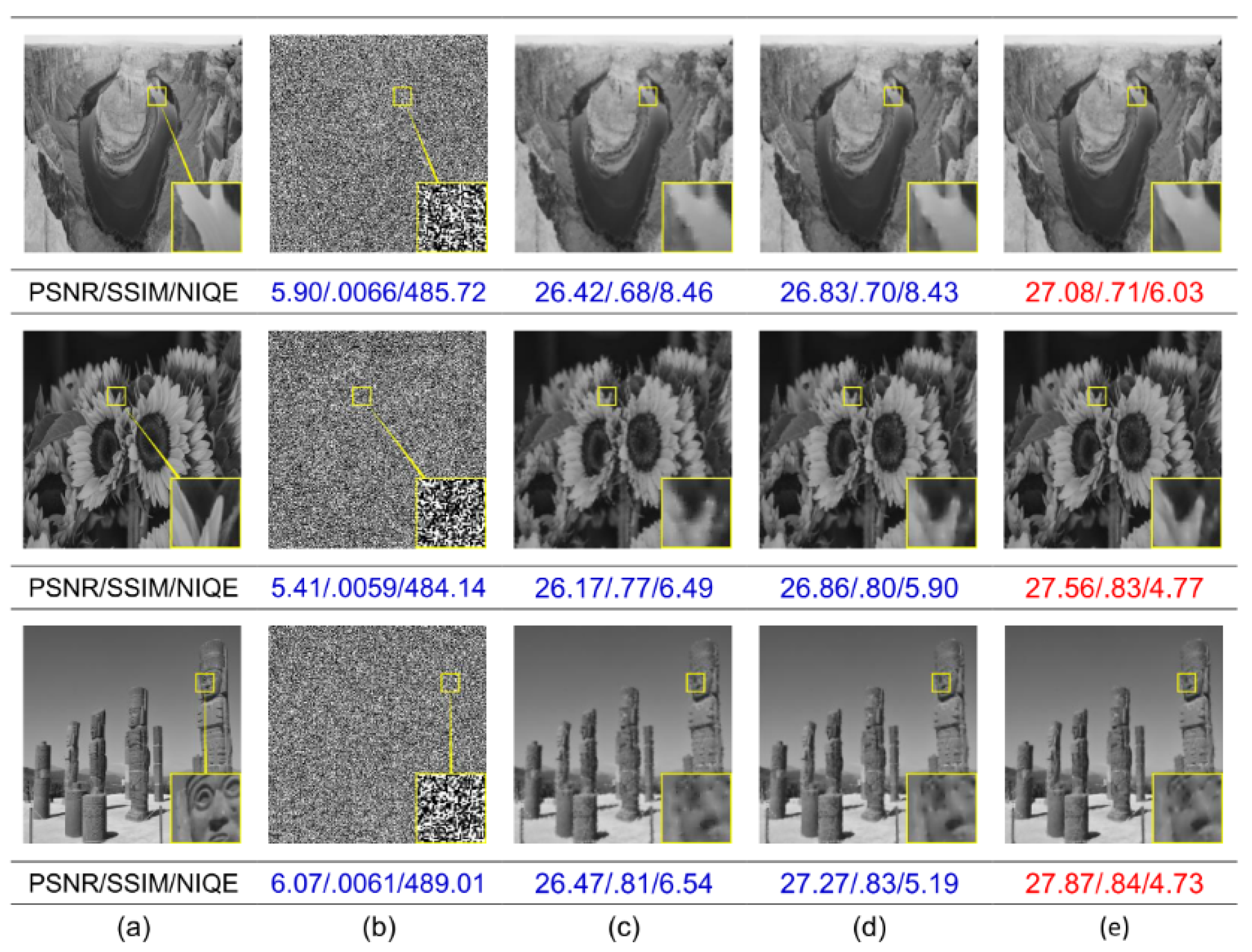
  • We conduct extensive experiments to compare our method with state-of-the-art image denoising methods using the DIV2k dataset [18] to demonstrate the superiority and effectiveness of the proposed denoising framework qualitatively and quantitatively.
The rest of the paper is organized as follows. In Section 2, the related work will be discussed. The proposed method is described in detail in Section 3. Section 4 introduces the experimental environment and analyzes the results. Section 5 concludes the paper.

2. Related Work

2.1. Denoising with Conventional Linear or Nonlinear Filtering

Denoising using linear filtering [19] replaces a noisy pixel with the average of the neighboring image pixels surrounding a noisy one. However, average filtering that includes noise pixels creates artifacts in denoised results. Furthermore, it causes blurring since it replaces a noisy pixel with the mean value of the filter kernel. For nonlinear filters, one of the most commonly used ones for impulse noise is the median filter [4], which replaces noisy pixels with the median value of the filter kernel. Median filtering can preserve more edges and details than average filtering. However, it may also produce artifacts, such as jagged edges. As the filter kernel size grows bigger due to higher-density noise, the image would also be blurred. Therefore, weighted median filtering [20] was proposed to reduce blurriness when using larger kernels. Since preserving image details while removing noisy pixels is critical in denoising, bilateral filtering [21,22], which utilizes Gaussian-based spatial and range kernels, considers pixel differences, meaning larger pixel differences result in small weights while smoothing to preserve possible edges. Nevertheless, it does not work for impulse noise since noisy pixels usually are much more different from good pixels, thus not filtered. Unlike these filters, we propose to use adaptive and overlapped average filtering, which selects an appropriate kernel size based on the noise density and smooth noisy pixels in an overlapped manner, performing exceptionally well for images with high-density noise.

2.2. Denoising with Deep Neural Networks
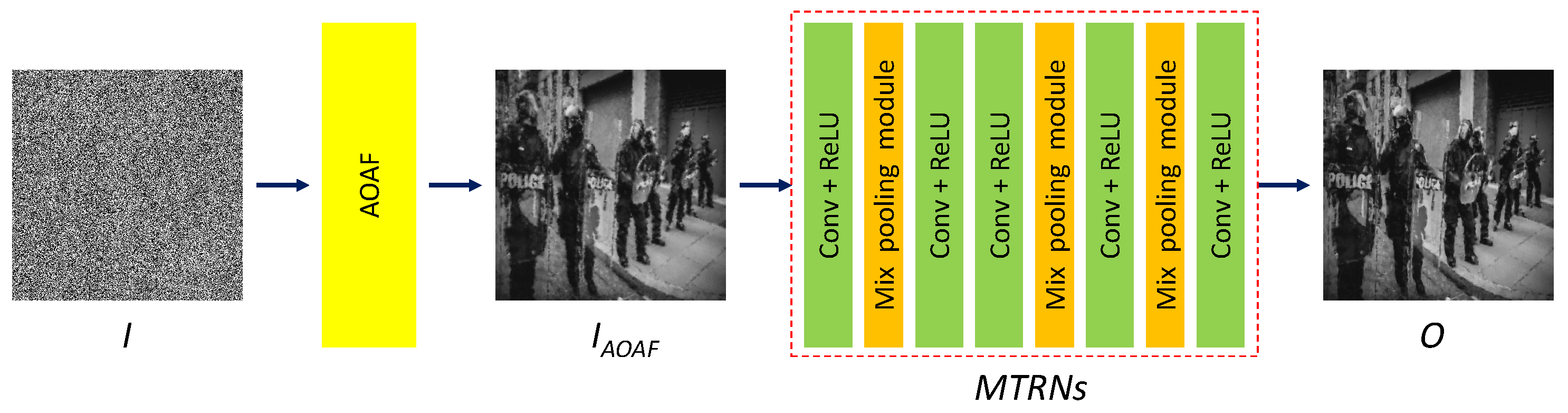
In recent years, deep learning has achieved great success in image processing applications. In contrast to conventional filtering, deep learning has also been applied to denoising. Zhang et al. [23] proposed feed-forward denoising convolutional neural networks, which use residual learning and batch normalization to boost denoising performance. Xing et al. [16] proposed to remove SP noise using multiple denoisers implemented using convolutional neural networks, each of which is for a different noise scale. However, it may introduce jagged edges in the denoised results, making the denoised images not natural. Ulyanov et al. proposed Deep Image Prior [15], which uses a deep autoencoder to restore images with noise through self-supervised learning, but it does not work for impulse noise. Laine’s method [17] backbones a convolutional blind-spot network, where the noisy center pixel in the receptive field is excluded for better denoising upon training. In addition, it builds a Bayesian model that uses the posterior mean and variance estimation to map a Gaussian approximation to the clean the prior based on noisy image observations. However, it only works for images with low- or moderate-density Gaussian or impulse noise but fails to repair images with high-density noise since there is no sufficient noise-free information for the model to recover noisy pixels. In general, using deep neural networks cannot perform well to remove high-density noise since it is difficult to learn random sparse non-noisy pixels to recover other noisy ones through training. Thus, we adopt deep neural networks to refine preliminary denoised results instead of dealing with noisy images directly to circumvent this issue.

3. Proposed Method

In the following, we introduce the proposed denoising framework in detail in two parts. First, we use the proposed AOAF to preliminarily smooth noisy pixels in an overlapped manner. Next, we design MARNs to refine the preliminary result and restore image details and edges. The whole denoising process includes two stages. In the first stage, we apply AOAF to the noisy image to eliminate all the noisy pixels and initially restore the noisy pixels. In the second stage, the proposed MARNs refine the preliminarily denoised result to recover image details and textures, making the denoised result natural and distortion-free. Figure 1 shows the flowchart of the proposed framework.

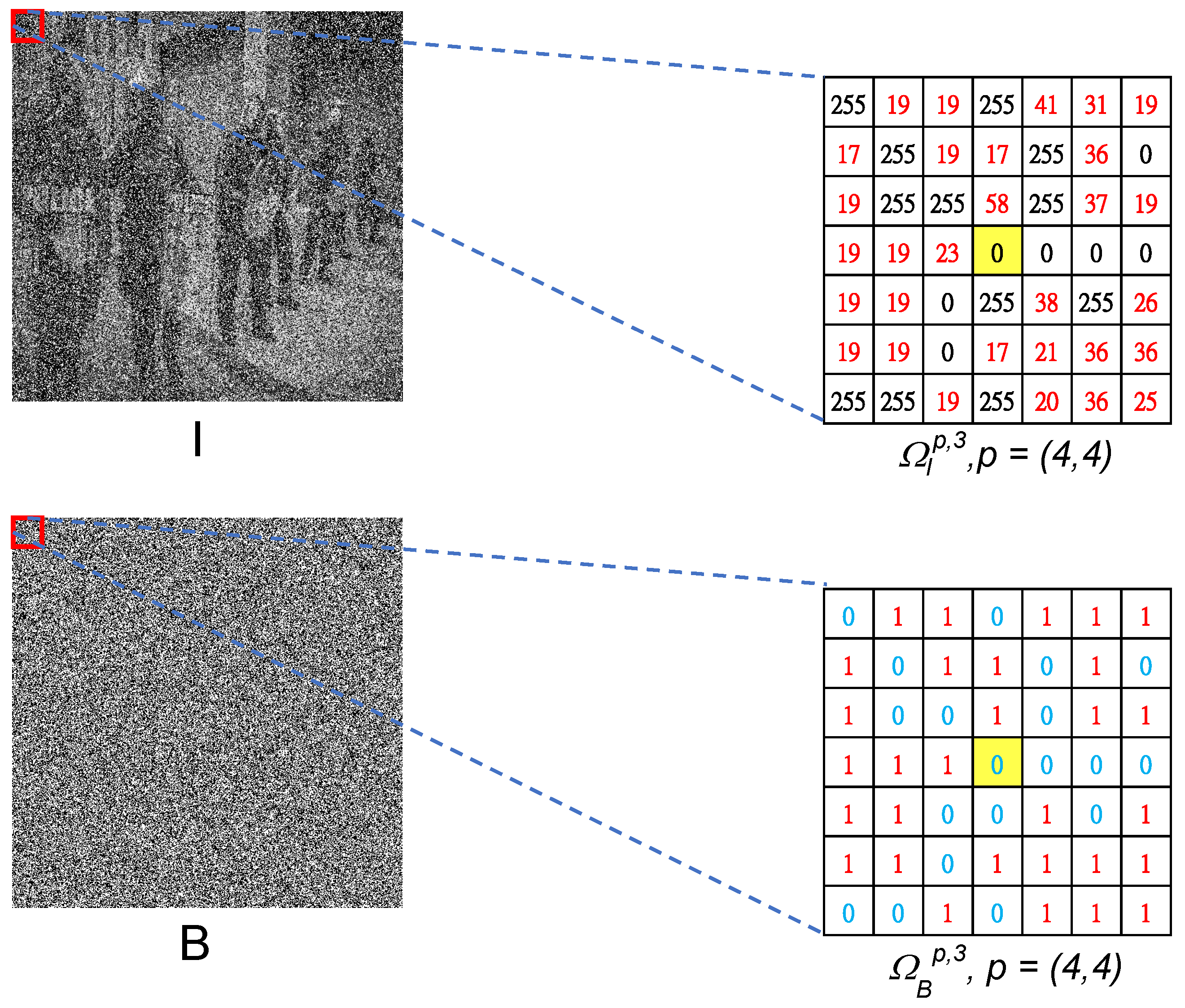
3.1. Adaptive and Overlapped Average Filter (AOAF)

The AOAF is essentially used to determine the kernel size adaptively and to perform average filtering in an overlapped fashion. We detail the proposed AOAF in Algorithm 1. Let N be the total number of pixels, I is the noisy input image, I A O A F represents the denoised output image, and ⊗ and . / represent the multiplication and division of individual elements.
Algorithm 1 Adaptive and Overlapped Average Filter (AOAF)
Input: 
Noisy image I R N
Output: 
Denoised image I A O A F R N
1:
C B
2:
T B I
3:
for each noisy pixel coordinate p in I do
4:
     r Find_Kernel_Radius(I, p)
5:
    pAvg equals the average of all the non-noise pixels in Ω I p , r
6:
    for each pixel coordinate i in  Ω I p , r
7:
        if  Ω I p , r ( i ) is a noisy pixel then
8:
            C ( i ) C ( i ) + 1
9:
            T ( i ) T ( i ) + p A v g
10:
        end if
11:
    end for do
12:
end for
13:
I A O A F T . / C
14:
return I A O A F
For an image with SP noise, a noisy pixel has either the highest or lowest intensity, normalized to be 1 and 0. We construct a non-noisy map B Z N for the input image I R N as
B ( i ) = 0 , I ( i ) = 0 o r 1 ; 1 , o t h e r w i s e ,
where i is a pixel coordinate. In Algorithm 1, C B means we assign B to C. In our implementation, we declare both of them arrays. Thus, we can copy all the elements in B to C. We declare a temporary array, denoted as T, to save accumulated filtered results, initialized with B I to extract all the non-noisy pixels.
The function Find _ Kernel _ Radius determines the size of the filter kernel ( 2 r + 1 ) 2 , where r is the radius of the kernel, initially set to 1. For a noisy pixel with the coordinate of p, if no non-noisy pixel is found in the ( 2 r + 1 ) 2 window centered at p, the radius r will increase by 1. The window keeps enlarging until at least one non-noisy pixel is found in it. The final window size determines the radius of the kernel. The average kernel with the radius of r can be expressed as:
K a v g r = 1 ( 2 r + 1 ) 2 1 1 1 1 1 1 1 1 1 1 1 1 1 1 1 1 R ( 2 r + 1 ) × ( 2 r + 1 ) ,
where K a v g r is a two-dimensional square matrix with all its elements the same as 1 ( 2 r + 1 ) 2 where 1 r 19 . The kernel is convolved with the window centered at a pixel coordinate p in I, expressed as Ω I p , r , meaning applying average filtering with K a v g r to the image window of the same size of the kernel. The convolution result p A v g can be derived by:
p A v g = ( Ω I p , r Ω B p , r ) K a v g r Ω B p , r K a v g r = i Ω I p , r ( i ) × Ω B p , r ( i ) × K a v g r ( i ) j Ω B p , r ( j ) × K a v g r ( j ) = i Ω I p , r ( i ) × Ω B p , r ( i ) j Ω B p , r ( j ) ,
where ⊙ represents the convolution operator, and Ω B p , r is the window centered at the pixel coordinate p in the non-noisy map B . To better understand these local windows center at p, we use Figure 2 as an example of 7 × 7 square windows ( r = 3 ) centered at the pixel coordinate of ( 4 , 4 ) in a noisy image I and its corresponding non-noisy map B .
Next, we consider p A v g as a denoised candidate for each noisy pixel in the window Ω I p , r and accumulate the average value in a temporary result T (as Algorithm 1 on the line of T ( i ) T ( i ) + p A v g ). We use the counter map C Z N corresponding to T ( i ) to record the number of times the noisy pixels are accumulated ( C ( i ) C ( i ) + 1 ). The final denoised result I A O A F equals T divided element-wisely by the cumulative number of denoised candidates C as I A O A F = T . / C .

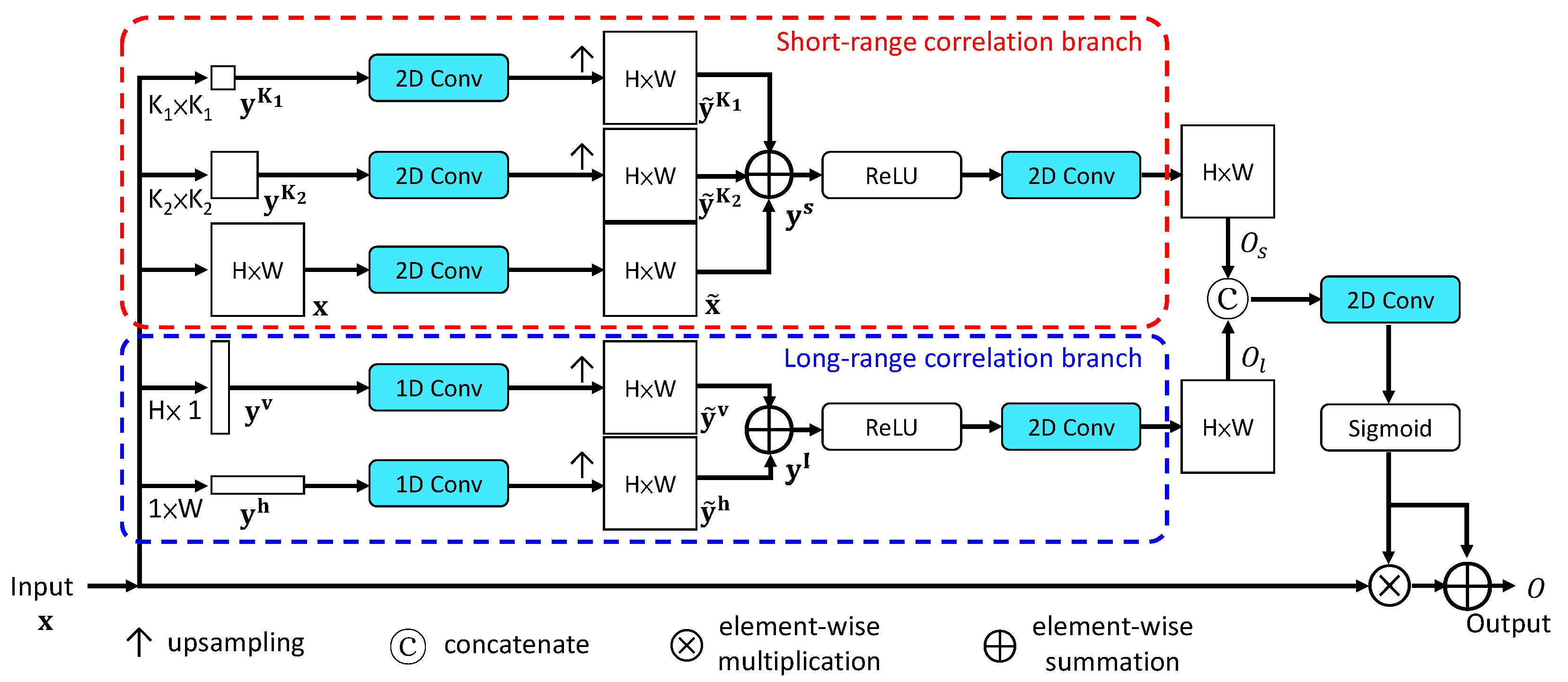
3.2. Mixed-pooling Attention Refinement Networks (MARNs)

Followed by AOAF, the proposed MTRNs refines the preliminary filtered result to restore corrupted fine details in the denoised images. The MTRNs include five 3 × 3 convolutional layers (Conv) with the ReLU activation function and three mixed pooling modules [24] that function as attention layers. For the five convolutional layers, except for the first and last layers, the number of channels is 64. The number of channels in the first and last layers equals the number of image channels (one for a grayscale image and three for a color image). The loss function is the mean square error between the estimated denoised image and the noise-free ground-truth image. The detailed architecture is shown in Figure 1.
To better restoring noisy images, we adopt the mixed pooling module (MPM) [24] functioning as a self-attention model, consisting of two branches that simultaneously capture short-range and long-range correlations between pixels across the entire image, shown in Figure 3. For the short-range correlation branch, pyramid pooling is used to collect short-distance dependencies. Let the input tensor be x R H × W × C , where H and W represent the tensor height and width, and C is the number of channels. In pyramid pooling, it stacks two adaptive average pooling layers in parallel to produce y K z R K z × K z × C as:
y i , j , c K z = 1 s v z × s h z m = 0 s v z 1 n = 0 s h z 1 x ( i × s v z ) , ( j × s h z ) , c ,
where z = 1 or 2, s v z = H + K z 1 K z , s h z = W + K z 1 K z . Here, we set K 1 = 12 and K 2 = 20 . Next, after applying a 3 × 3 2D convolution, denoted as f 3 × 3 ( · ) , to y K 1 , y K 2 , and x , we obtain y ˜ K 1 = f 3 × 3 ( y K 1 ) , y ˜ K 2 = f 3 × 3 ( y K 2 ) , and x ˜ = f 3 × 3 ( x ) . Then, they are upsampled and merged as:
y i , j , c s = x ˜ i , j , c + z = 1 2 y ˜ i + K z 1 K z , j + K z 1 K z , c K z ,
where y s R H × W × C .
The long-range correlation branch adopts strip pooling to collect long-distance dependencies across the entire input. Applying horizontal and vertical strip pooling to the input tensor x generates H × 1 and 1 × W outputs, y v R H × C and y h R W × C as:
y i , c v = 1 W j = 0 W 1 x i , j , c s , 1 i H ; y j , c h = 1 H i = 0 H 1 x i , j , c s , 1 j W .
Next, after applying a 3 × 1 1D convolution, denoted as f 3 × 1 ( · ) , to y h and 1 × 3 1D convolution f 1 × 3 ( · ) to y v , we obtain y ˜ h = f 3 × 1 ( y h ) and y ˜ v = f 1 × 3 ( y v ) . Then, they are upsampled and merged as y i , j , c l = y ˜ i , c v + y ˜ j , c h , where y l R H × W × C .
In each branch, outputs are upsampled to the original input size H × W and merged by summation, followed by the ReLU activation function σ r e l u and another 3 × 3 convolution. The output for the short-range correlation branches is denoted as O s = f 3 × 3 ( σ r e l u ( y s ) ) , and that for the long-range, O l = f 3 × 3 ( σ r e l u ( y l ) ) . The two branches’ outputs are concatenated and convolved with a 3 × 3 convolution and then passed through the sigmoid function σ s i g to turn into attention maps. The final MPM output O is given as:
O = I I σ s i g ( f 3 × 3 ( O s O l ) ) ,
where ⊕, ⊗, and ‖ represent element-wise summation, element-wise multiplication, and concatenation, respectively. Adopting MPMs in our model can emphasize the image details more, such as edges, shapes, and textures, and make denoising results look more natural.

4. Experimental Results

4.1. Settings for Training and Testing

For training the MARNs and testing our denoising framework, we used the grayscale version of the DIV2K dataset [18], where it contains 800 high-definition and high-resolution images collected from the Internet. These images were divided into training and test datasets, which contain 600 and 200 images, respectively. All images were resized to 512 × 512 . Since it is relatively easy for most existing methods to denoise images with less than 50% SP noise, we tested denoising capacity with higher-density SP noise. Thus, we simulated noisy images with various noise density levels by randomly adding 50%, 60%, 70%, 80%, and 90% SP noise to images. Note that our method works well for lower-density SP noise, even though this was not included in our training dataset. There were 3000 (600 images × 5 noise levels) images generated to train the MARNs and 1000 (200 images × 5 noise levels) for testing. Note that we used 1000 test images to generate all the experimental results, including Figure 4, Figure 5 and Figure 6 and Table 1 and Table 2. We adopted the Adam optimizer with a fixed learning rate of 1 × 10⁻³ and ran 80 epochs to train our networks. All the experiments were run on a desktop with Amd Ryzen 7 3700× 3.6 GHz CPU, 64GB RAM, and an Nvidia GeForce RTX 3090 Ti with 24GB of VRAM.

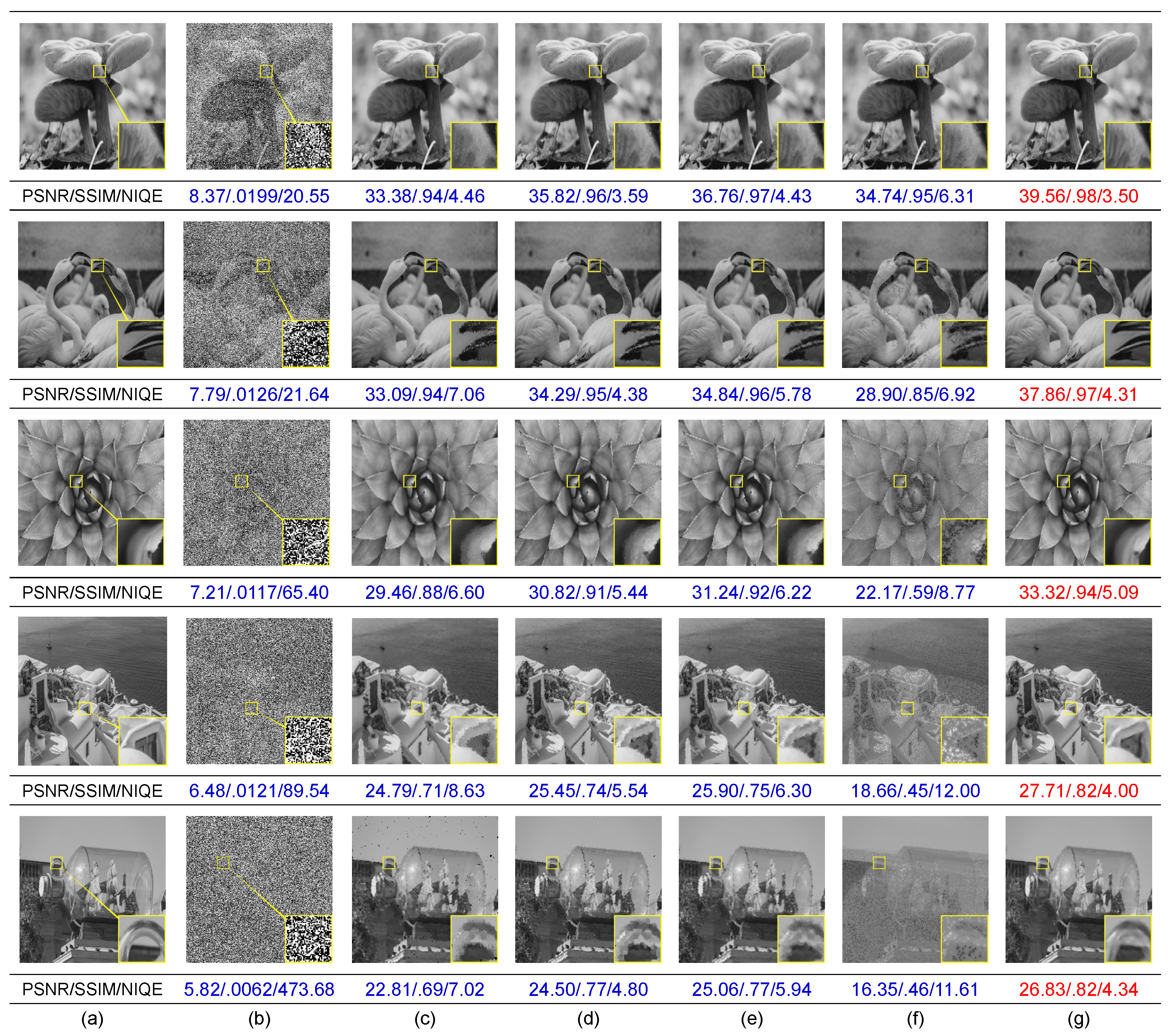
4.2. Comparisons of Benchmark Methods

We conducted experiments to evaluate the performance with two full-reference metrics (PSNR, SSIM) and one no-reference metric (NIQE). PSNR represents pixel similarity, SSIM measures similarity of luminance, contrast, and structure, and NIQE could represent image naturalness. For both PSNR and SSIM [25], a more significant value means a higher similarity between a denoised image and its noise-free version. The Natural Image Quality Evaluator (NIQE) [26] is an entirely blind image quality analyzer that uses space-domain natural scene statistics to evaluate an image’s visual quality. A small value of the NIQE represents a better quality.
We compared our proposed framework against four state-of-the-art SP denoising methods, including MDBUTMF [8], DAMF [9], FASMF [10], and MMAP [11], quantitatively and qualitatively. Note that since MMAP [11] does not release code, we used our implementation. As shown in Figure 4, we can see that denoising with MDBUTMF [8], DAMF [9], FASMF [10], and MMAP [11] can remove 50–90% of SP noise. For the noise level of 50%, all these methods can produce good denoising results. However, they did not do well in restoring image details and even produced jagged edges. MMAP [11] denoises images with a small kernel size, not working well for high-density noise. By contrast, the proposed framework performs much better than the other compared methods, making the denoising results look like original, noise-free, high-definition and high-resolution images. Figure 5 shows the denoising results for color images. Since all the compared methods are designed to work for images with a single channel, we apply a denoising method to each of the red, blue, and green channels individually for color image denoising. Again, our method performs the best with degraded image edges and details reconstructed in color image denoising. Figure 6 demonstrates more denoising results with the most challenging cases (90% noise), where we can see the proposed method can restore noisy images with a variety of contents.
Table 1 shows the objective quality comparisons of all the compared methods, where all the scores are averaged over the test dataset. As seen, denoising with the proposed AOAF only achieves better results for images with over 70% noise than MDBUTMF [8], DAMF [9], FASMF [10], and MMAP [11]. For images with 50% and 60% noise, AOAF performs comparably against the second-best method, FASMF [10], in PSNR and SSIM since most denoising methods work fine with less noise but not for more challenging cases (more than 70% noise). AOAF can generate more smooth denoising results with overlapping averaging. Note that since NIQE favors sharp images, AOAF does not have the best score here. Even though the other methods [8,9,10] have better NIQE scores, they generated fake edges, presenting unreal denoising images, as shown in Figure 4, Figure 5 and Figure 6. Our denoising framework that cascades AOAF and MARNs works best in PSNR, SSIM, and NIQE on average. Table 2 shows an ablation study of the proposed framework, where all the scores are averaged over the test dataset. As can be seen, denoising with AOAF followed by only five convolutional layers without MPMs (AOAF+Conv) works better than using AOAF only. Using MARNs with AOAF (AOAF+Conv+MPMs) performs even better, demonstrating that utilizing the attention mechanism in denoising leads to a significant gain. Figure 7 shows that AOAF can remove SP noise and rudimentarily restore images. AOAF’s results passing through five convolutional layers are a little sharper but still blurred. Combining AOAF with the designed MARNs can further refine the results to achieve higher visual quality. Therefore, AOAF plus MARNs can restore images with high-density SP noise, making the denoising results look natural and as though the image was never degraded. Cascading AOAF and MARNs has proven an effective framework in denoising.

5. Conclusions

This paper proposed an effective denoising framework that cascades AOAF and MARNs to remove high-density SP noise and restore image details. Applying AOAF to the noisy input image produces the preliminarily denoised result with noisy pixels removed and recovered, followed by MTRNs to refine the preliminary result to reconstruct image details. The proposed method performs favorably against state-of-the-art denoising methods for a wide range of high densities of SP noise in images.

Author Contributions

Conceptualization, methodology, software, and validation, M.-H.L., Z.-X.H., and K.-H.C.; experiment analysis, Z.-X.H.; investigation and writing—original draft preparation, M.-H.L. and Z.-X.H.; proofreading and editing, Y.-T.P.; supervision, C.-H.W. and Y.-T.P.; project administration, Y.-T.P.; funding acquisition, Y.-T.P. All authors have read and agreed to the published version of the manuscript.

Funding

This paper was supported in part by the Ministry of Science and Technology, Taiwan (MOST) under Grant No. MOST109-2221-E-004-014, No. MOST110-2634-F-019-001 and No. MOST110-2634-F-004-001 through Pervasive Artificial Intelligence Research (PAIR) Labs.

Institutional Review Board Statement

Not applicable.

Informed Consent Statement

Not applicable.

Data Availability Statement

Publicly available datasets were adopted in this study. This data can be found here: https://data.vision.ee.ethz.ch/cvl/DIV2K/ (accessed on 16 March 2021).

Conflicts of Interest

The funders had no role in the design of the study; in the collection, analyses, or interpretation of data; in the writing of the manuscript, or in the decision to publish the results.

Abbreviations

Acronyms used in the paper:
AOAFAdaptive and Overlapped Average
MARNsMixed-pooling Attention Refinement Network
MDBUTMFModified Decision-Based Unsymmetrical Trimmed Median Filter
DAMFDifferent Applied Median Filter
FASMFFast Adaptive and Selective Mean Filter
MMAPMin-Max Average Pooling
CNNconvolutional neural networks
NIQENatural Image Quality Evaluator

References

  1. Huang, S.C.; Peng, Y.T.; Chang, C.H.; Cheng, K.H.; Huang, S.W.; Chen, B.H. Restoration of Images With High-Density Impulsive Noise Based on Sparse Approximation and Ant-Colony Optimization. IEEE Access 2020, 8, 99180–99189. [Google Scholar] [CrossRef]
  2. Chen, H.J.; Ruan, S.J.; Huang, S.W.; Peng, Y.T. Lung X-ray Segmentation using Deep Convolutional Neural Networks on Contrast-Enhanced Binarized Images. Mathematics 2020, 8, 545. [Google Scholar] [CrossRef]
  3. Yang, H.; Wang, J.; Miao, Y.; Yang, Y.; Zhao, Z.; Wang, Z.; Sun, Q.; Wu, D.O. Combining spatio-temporal context and Kalman filtering for visual tracking. Mathematics 2019, 7, 1059. [Google Scholar] [CrossRef] [Green Version]
  4. Astola, J.; Kuosmanen, P. Fundamentals of Nonlinear Digital Filtering; CRC Press: Boca Raton, FL, USA, 1997. [Google Scholar]
  5. Toh, K.K.V.; Isa, N.A.M. Noise adaptive fuzzy switching median filter for salt-and-pepper noise reduction. Signal Process. Lett. 2009, 17, 281–284. [Google Scholar] [CrossRef] [Green Version]
  6. Zhang, S.; Karim, M.A. A new impulse detector for switching median filters. Signal Process. Lett. 2002, 9, 360–363. [Google Scholar] [CrossRef]
  7. Ng, P.E.; Ma, K.K. A switching median filter with boundary discriminative noise detection for extremely corrupted images. IEEE Trans. Image Process. 2006, 15, 1506–1516. [Google Scholar] [PubMed]
  8. Esakkirajan, S.; Veerakumar, T.; Subramanyam, A.N.; PremChand, C. Removal of high density salt and pepper noise through modified decision based unsymmetric trimmed median filter. Signal Process. Lett. 2011, 18, 287–290. [Google Scholar] [CrossRef]
  9. Erkan, U.; Gökrem, L.; Enginoğlu, S. Different applied median filter in salt and pepper noise. Comput. Electr. Eng. 2018, 70, 789–798. [Google Scholar] [CrossRef]
  10. Fareed, S.B.S.; Khader, S.S. Fast adaptive and selective mean filter for the removal of high-density salt and pepper noise. IET Image Process. 2018, 12, 1378–1387. [Google Scholar] [CrossRef]
  11. Satti, P.; Sharma, N.; Garg, B. Min-Max Average Pooling Based Filter for Impulse Noise Removal. Signal Process. Lett. 2020, 27, 1475–1479. [Google Scholar] [CrossRef]
  12. Chen, F.; Ma, G.; Lin, L.; Qin, Q. Impulsive noise removal via sparse representation. J. Electron. Imaging 2013, 22, 043014. [Google Scholar] [CrossRef]
  13. Aggarwal, H.K.; Majumdar, A. Exploiting spatiospectral correlation for impulse denoising in hyperspectral images. J. Electron. Imaging 2015, 24, 013027. [Google Scholar] [CrossRef]
  14. Yin, J.L.; Chen, B.H.; Li, Y. Highly accurate image reconstruction for multimodal noise suppression using semisupervised learning on big data. IEEE Trans. Multimed. 2018, 20, 3045–3056. [Google Scholar] [CrossRef]
  15. Ulyanov, D.; Vedaldi, A.; Lempitsky, V. Deep image prior. In Proceedings of the Conference on Computer Vision and Pattern Recognition, Guangzhou, China, 23–26 November 2018. [Google Scholar]
  16. Xing, Y.; Xu, J.; Tan, J.; Li, D.; Zha, W. Deep CNN for removal of salt and pepper noise. IET Image Process. 2019, 13, 1550–1560. [Google Scholar] [CrossRef]
  17. Laine, S.; Karras, T.; Lehtinen, J.; Aila, T. High-quality self-supervised deep image denoising. In Proceedings of the Neural Information Processing Systems, Vancouver, BC, Canada, 8–14 December 2019. [Google Scholar]
  18. Agustsson, E.; Timofte, R. Ntire 2017 challenge on single image super-resolution: Dataset and study. In Proceedings of the Conference on Computer Vision and Pattern Recognition Workshops, Honolulu, HI, USA, 21–26 July 2017. [Google Scholar]
  19. Kong, L.; Wen, H.; Guo, L.; Wang, Q.; Han, Y. Improvement of linear filter in image denoising. In Proceedings of the International Conference on Intelligent Earth Observing and Applications 2015, Guilin, China, 23–24 October 2015. [Google Scholar]
  20. Brownrigg, D.R. The weighted median filter. Commun. ACM 1984, 27, 807–818. [Google Scholar] [CrossRef]
  21. Tomasi, C.; Manduchi, R. Bilateral filtering for gray and color images. In Proceedings of the Sixth International Conference on Computer Vision (IEEE Cat. No. 98CH36271), Bombay, India, 7 January 1998. [Google Scholar]
  22. Francis, J.; De Jager, G. The bilateral median filter. In Proceedings of the 14th Annual Symposium of the Pattern Recognition Association of South Africa, Langebaan, South Africa, 27–28 November 2003. [Google Scholar]
  23. Zhang, K.; Zuo, W.; Chen, Y.; Meng, D.; Zhang, L. Beyond a Gaussian Denoiser: Residual Learning of Deep CNN for Image Denoising. IEEE Trans. Image Process. 2017, 26, 3142–3155. [Google Scholar] [CrossRef] [PubMed] [Green Version]
  24. Hou, Q.; Zhang, L.; Cheng, M.M.; Feng, J. Strip pooling: Rethinking spatial pooling for scene parsing. In Proceedings of the Conference on Computer Vision and Pattern Recognition, Seattle, WA, USA, 14–19 June 2020. [Google Scholar]
  25. Zhou, W. Image quality assessment: From error measurement to structural similarity. IEEE Trans. Image Process. 2004, 13, 600–613. [Google Scholar]
  26. Mittal, A.; Soundararajan, R.; Bovik, A.C. Making a “completely blind” image quality analyzer. Signal Process. Lett. 2012, 20, 209–212. [Google Scholar] [CrossRef]
Figure 1. Flowchart of the proposed denoising framework.
Mathematics 09 01130 g001
Figure 2. An example of square windows centered at a pixel coordinate p in a noisy image I and the corresponding non-noisy map B , denoted as Ω I p , r and Ω B p , r , respectively. Here, p = ( 4 , 4 ) and r = 3 .
Mathematics 09 01130 g002
Figure 3. The Mixed Pooling Module (MPM) [24].
Mathematics 09 01130 g003
Figure 4. Examples of denoising results for images with 50-90% noise added using different methods. We show the corresponding objective scores below the measured images. The best scores are in red. (a) Original image. (b) Images with 50%, 60%, 70%, 80%, 90% noise added (from the top to bottom rows). Denoising results using (c) MDBUTMF [8], (d) DAMF [9], (e) FASMF [10], (f) MMAP [11], and (g) the proposed (AOAF+MARNs).
Mathematics 09 01130 g004
Figure 5. Examples of denoising results for color images with 50-90% noise added using different methods. We show the corresponding objective scores below the measured images. The best scores are in red. (a) Original image. (b) Images with 50%, 60%, 70%, 80%, 90% noise added (from the top to bottom rows). Denoising results using (c) MDBUTMF [8], (d) DAMF [9], (e) FASMF [10], (f) MMAP [11], and (g) the proposed (AOAF+MARNs).
Mathematics 09 01130 g005
Figure 6. More examples of denoising results for images with 90% noise added using different methods. We show the corresponding objective scores below the measured images. The best scores are in red. (a) Original image. (b) Noisy images. Denoising results using (c) MDBUTMF [8], (d) DAMF [9], (e) FASMF [10], (f) MMAP [11], and (g) the proposed (AOAF+MARNs).
Mathematics 09 01130 g006
Figure 7. Ablation study of the proposed denoising framework based on subjective comparisons. We show the corresponding objective scores below the measured images. The best scores are in red. (a) Original image. (b) Image with 90% noise added. Denoising results using (c) AOAF, (d) AOAF+Conv, and (e) AOAF+Conv+MPMs.
Mathematics 09 01130 g007
Table 1. Objective quality comparisons of all the compared methods. All the scores are averaged over the test dataset. The best score in each column is marked in red and the second-best in blue.
PSNR↑SSIM↑NIQE↓
Noise Level50%60%70%80%90%50%60%70%80%90%50%60%70%80%90%
MDBUTMF [8]27.8526.8725.9124.8422.040.860.820.780.730.615.776.958.058.237.55
DAMF [9]29.9028.5427.1825.6723.490.910.880.840.780.694.905.215.315.345.66
FASMF [10]30.4929.1127.6826.0824.050.920.890.840.780.685.185.746.346.465.99
MMAP [11]29.9423.7119.3417.4915.780.900.680.490.410.357.157.978.9710.9214.69
AOAF30.0229.0227.9426.6524.830.900.880.840.790.716.897.818.278.187.59
AOAF+MARNs32.8331.5129.9828.1825.740.940.920.890.840.753.763.944.104.495.51
Table 2. Ablation study of the proposed framework. All the scores are averaged over the test dataset. The best score in each column is marked in red and the second-best in blue.
PSNR↑SSIM↑NIQE↓
Noise Density50%60%70%80%90%50%60%70%80%90%50%60%70%80%90%
AOAF30.0229.0227.9426.6524.830.900.880.840.790.716.897.818.278.187.59
AOAF+Conv31.9630.7629.3127.5625.250.930.910.880.830.744.344.745.286.167.59
AOAF+Conv+MPMs32.8331.5129.9828.1825.740.940.920.890.840.753.763.944.104.495.51
Publisher’s Note: MDPI stays neutral with regard to jurisdictional claims in published maps and institutional affiliations.

