Preventive Maintenance of the k-out-of-n System with Respect to Cost-Type Criterion

Abstract

In a previous paper, the problem of how the preventive maintenance organization for the k-out-of-n: F system could be used, in order to maximize system availability, was considered. The current paper continues these investigations using a different optimization criterion. The proposed approach is based on decision making theory for regenerative processes. We propose a general procedure for comparing different preventive maintenance strategies based on the ordered statistics distributions, aiming to choose the best one with respect to cost-type criterion. The lifetime distributions of system units are usually unknown and only one or two of their moments are available. For this reason, we pay special attention to the sensitivity analysis of decision making about preventive maintenance, taking into account the shape of the system unit lifetime distributions. A numerical study of two examples based on a real-world system illustrates the results of the proposed approach.

1. Introduction and Motivation

Ensuring the reliability of systems, objects, and processes is one of the main problems that must be solved during their creation and further operation. One of the ways to improve their reliability is redundancy. A k-out-of-n: F model represents a system of n parallel-connected units that fails when at least k of them fail. It can be considered as one of the types of redundancy configuration. Such models are used in various fields of human activity: their application can be seen in many real-world phenomena, including telecommunications, transmissions, engineering constructions, transport, manufacturing, services, etc. Due to the widespread areas of practical applications, a large number of papers have been devoted to the study of k-out-of-n: F systems. The bibliography (on publications about these systems) is extensive (see Trivedi [1], Chakravarthy et al. [2] and the bibliography therein). For a brief overview of further investigations on this topic, please see, for example, [3]. An overview of recent publications on k-out-of-n multi-state systems can be found in [4]. Engineering applications of this model used to study real-world systems can be found in [5] for the reliability of some structures in the oil and gas industry; for a remote monitoring system of underwater sections of gas pipeline [6]; for the reliability of a rotary-wing flight module of a high-altitude telecommunications platform [7].

Another method to improve the reliability of systems is preventive maintenance (PM) organization. The PM optimization problem is a part of the general theory of stochastic systems control. The latter originated and developed within the framework of the decision-making theory, in particular, the Markov Decision Process (MDP). One of the first research studies in this direction belongs to Kolmogorov, and was associated with product acceptance control. Famous scientists, such as as Bellman, Bleckwell, Derman, Dynkin, Ross, Shiryaev, and others, took part in the construction and development of this theory. An overview of the first steps in these investigations can be found in [8]. For the current state of research in this area, jointly with their applications, please look in [9].

Without going into detail, the main result of the MDP theory is as follows. The optimal strategy for MDP, with respect to additive optimization functional, belongs to the class on non-randomized Markov strategies. This result opens up some perspectives for constructing optimal strategies, and specific numerical methods. The basic ideas have been developed by Howard [10], Wolf, and Danzig [11], and can be found in some monographs, for example [12].

Regular applications of the theory of controllable random processes to queuing and reliability models began with [13], (see also [14]). There, for the first time, a definition of the concept of the controllable queuing system was proposed, and an overview of the earlier investigations on this topic was given. Later, several special monographs appeared, analyzing this topic [15,16,17] and others.

As a part of the general theory of the stochastic systems control, the specificity of applications of the PM optimization problem leaves an imprint on their formulations and ways for solutions. One can find an overview of various approaches and results of studying PM of complex stochastic systems in Gertsbakh’s monograph [18]. There are different types of PM scenarios based on the possibility of observing system states, available information about the system, and other factors. Some of these scenarios are: (a) periodic replacement of units; (b) age replacement of units; (c) PM based on system state observation.

Other scenarios are also possible, and different criteria are used for the best PM choice.

In a series of papers by Dudin, Krishnamurthy, et al. [19,20,21,22,23,24], the k-out-of-n non-reliable queuing system with different types of service and repair strategies were considered. Some optimal opportunistic maintenance strategies were introduced and investigated in [25,26]. As for the development of the multi-state system—one can find it in [27]. Recent developments on optimal PM policies can be found in [28,29,30,31,32]. For a review on the recent investigations on maintenance optimization, see [33].

Usually the detailed initial information about lifetimes of the system units is not available, and only one or two of their moments are known. Therefore it is fundamentally important to study the sensitivity of the system reliability indicators with respect to the shape of their unit lifetime distributions. Research in this direction can be found in a series of our papers, references to which one can find in chapter 9 of [34], as well as in [3]. For an overview of the recent research methods for queuing and reliability systems, one can find it in [35].

Most research assumes that any system PM and repair lead to its full renovation. This means that, after each complete repair, the system becomes as “new”. As a result of this assumption, the mathematical formulation of the problem can be conducted within the framework of regenerative or semi-regenerative processes. In [6], the problem of PM organization for the k-out-of-n: F system was considered with respect to system availability maximization. The present paper continues the ideas of previous investigations with the aim of developing a mathematical model for organizing the best PM for this system, with respect to a cost-type criterion and the available information. The novelty and features of this study are:

• A method for PM investigations of k-out-of-n: F systems, whose failures depend on the positions of failed units developed;
• A new approach based on ordered statistics is used to solve the problem;
• A cost-type criterion for PM strategies comparison is used;
• A study of the sensitivity of decision making to the type of system unit lifetime distribution is carried out.

The paper is organized as follows. In the next section, the formulation of the problem and notations and assumptions are presented. Further, in Section 3, the main result concerning comparisons between different PM strategies and the strategy “to work up to the system failure“, jointly with the appropriate algorithm, are presented. In the last Section 4, some numerical results and their graphic illustrations are presented for the system considered in [6], with respect to the cost-type criterion. Thus, here we use the same notation and descriptions.

2. The Problem Set Up, Assumptions, and Notations

2.1. Notations and Assumptions

Consider a k-out-of-n: F system, whose failures depend on the location of its failed units. Let us denote by $A_i:i=1,2,\cdots$ a sequence of system unit random lifetimes. Suppose that they are independent, identically distributed (i.i.d.) random variables (r.v.s) with common cumulative distribution function (c.d.f) $A\left(t\right)=\mathbf{P}\{A_i\le t\}$. After any system failure, it is repaired with a single facility, and the repair times are i.i.d. r.v.s $B_i^{\left(0\right)}:i=1,2,\cdots$ with common c.d.f. $B_0\left(t\right)=\mathbf{P}\{B_i^{\left(0\right)}\le t\}$.

To increase the productivity of the system, the possibility of PM based on the system state observation is considered. We denote by $\mathcal{L}=\{0,1,\cdots ,L\}$ the set of possible PM strategies, including running to the system failure for $l=0$. Let us denote by $E_l$ the subset of system states with l failed units. If the l-th PM begins after the l-th failure, then the set $E_l$ is the system “pre-failure” set, in which the l-th type of PM must be started. The times of PM are i.i.d. r.v.s $B_i^{\left(l\right)}$ with c.d.f. $B_l\left(t\right)=\mathbf{P}\{B_i^{\left(l\right)}\le t\}$. It is also supposed that the system gets a reward $\$c$ during the unit of its operating time, and pays the cost $\$c_0$ for its repair, and the cost $\$c_l$ for its PM per unit time. The quality of any PM strategy $l\in \mathcal{L}$ during time t is evaluated by

$$V_l\left(t\right)=\left\{\mathrm{the}\mathrm{income}\mathrm{of}\mathrm{the}\mathrm{system}\mathrm{operating}\mathrm{during}\mathrm{time}t\mathrm{for}l\in \mathcal{L}\right\}.$$

(1)

To describe the functioning of a complex system, whose failure depends not only on the number of its failed units, but also on their position in the system, let $\mathbf{j}=(j_1,j_2,\cdots j_n)$ be the system state, where $j_i=1$, if the i-th unit is in a failed state, and $j_i=0$, if it is in operational state. Thus, $j=j_1+\cdots +j_n$ is the number of failed system units. We also denote by

$$E=\{\mathbf{j}=(j_1,j_2,\cdots j_n):(j_i\in (0,1))\}$$

(2)

the set of all system states, and by $E_0$ and ${\overline{E}}_0$—subsets of its failed and operational states, accordingly. Note that the description of these sets is an application-specific problem, and should be considered in detail for each particular case.

The general assumptions are:

• At the very beginning the system is absolutely reliable, i.e., it is in zero state $\mathbf{j}=(0,\cdots ,0)$;
• All sequences of r.v.s (unit lifetimes, repair, and PM times) are i.i.d. for each type of r.v. Further, the letters without indexes are used for the representatives of appropriate sequence of r.v.s;
• The mean values of the unit lifetimes, as well as these for repair and PM times are finite,

  $$a=\mathbf{E}\left[A\right]<\infty ,b_0=\mathbf{E}\left[B^{\left(0\right)}\right]<\infty ,b_l=\mathbf{E}\left[B^{\left(l\right)}\right]<\infty .$$

  (3)
  It is supposed that the latter is less than the mean repair time, i.e., that $b_l\le b_0$, but may or may not depend on the type of PM;
• It is assumed that the mean unit lifetime, as well as the mean repair and PM times $b_0,b_l$ are known to the decision maker (DM);
• After any repair and PM completion, the system starts working “as a new one”, i.e., returns into the zero state. In other words, the model of the perfect PM is considered.

2.2. The Problem Set Up

The paper aims to investigate various PM strategies $l\in \mathcal{L}$, and the goal is to choose the best one with respect to the system average income per unit time to be maximized. The strategies $l=\{1,\cdots ,L\}$ are to start the PM when the system reaches the subset of states $S_l$ or to wait until the system fails for $l=0$. To solve the problem, we define a random process $\mathbf{J}=\left\{\mathbf{J}\right(t):t\ge 0\}$ with a space set E by the relation

$$\mathbf{J}\left(t\right)=\mathbf{j},\mathrm{if}\mathrm{at}\mathrm{time}t\mathrm{the}\mathrm{system}\mathrm{is}\mathrm{in}\mathrm{the}\mathrm{state}\mathbf{j}\in E.$$

(4)

Note that, due to our assumptions, the process $\mathbf{J}$ is regenerative under any PM strategy. Its regeneration epochs $\{S_0^{\left(l\right)}=0,S_i^{\left(l\right)}:i=1,2,\cdots \}$ are the times of the PM completion for $l=\{1,2,\cdots ,L\}$ and the repair completion for $l=0$. In other words, the values $S_i^{\left(l\right)}(l\in \mathcal{L})$ are the times until the process reaches the set of states $E_l$,

$$S_{i+1}^{\left(l\right)}=inf\{t:t>S_i^{\left(l\right)},\mathbf{J}\left(t\right)\in E_l\}.$$

(5)

Since the intervals $S_i^{\left(l\right)}-S_{i-1}^{\left(l\right)}$ are i.i.d. r.v.s, it is enough to study the process behavior only on one of them, for example, within the first one, $S_1^{\left(l\right)}$.

In the paper, we are interested in calculating various characteristics of the system, such as:

• System reliability function

  $$R\left(t\right)=\mathbf{P}\{S_1^{\left(0\right)}>t\}\mathrm{and}\mathrm{its}\mathrm{mean}\mathrm{value}{M}_0=\underset{0}{\overset{\infty }{\int }}R\left(t\right)dt.$$

  (6)
• Distributions of the times up to various PM starts and their mean values

  $$F_l\left(t\right)=\mathbf{P}\{S_1^{\left(l\right)}\le t\},M_l=\underset{0}{\overset{\infty }{\int }}(1-F_l\left(t\right))dt;$$

  (7)
• System quality measure $V_l$ for different PM strategies defined for $l\in \mathcal{L}$ as

  $$V_l=\underset{t\to \infty }{lim}\frac{1}{t}\mathbf{E}\left[V_l\left(t\right)\right].$$

  (8)

As a result, we compare different strategies with respect to the system quality $V_l$ and choose the best one.

Because the initial information about the system unit lifetime is usually very limited and available only up to knowledge of one, or two moments, our main focus is the study of the sensitivity of any decision about the PM quality, with respect to the shape of the system unit lifetime distributions.

3. The Problem Solution and the General Procedure for Comparing the Quality of PM Strategies

3.1. The Problem Solution

We should note that, due to our assumptions, the process $\mathbf{J}$ is a regenerative for any PM strategy $l\in \mathcal{L}$. Let us denote by ${\Pi }^{\left(l\right)}=S^{\left(l\right)}+B^{\left(l\right)}$ the process regeneration period for the system working under PM strategy $l\in \mathcal{L}$. Thus, the income $V_l\left(t\right)$ from the system operating during some time t under the PM strategy $l\in \mathcal{L}$ is

$$V_l\left(t\right)=\underset{0}{\overset{t}{\int }}[c{1}_{\{J\left(u\right)\in {\overline{E}}_l\}}-c_l{1}_{\{J\left(u\right)\in E_l\}}]du,$$

(9)

where $1_{\left\{A\right\}}$ is the indicator function of the event A and ${\overline{E}}_l=E\backslash E_l$. To calculate the long time average of mean income, we use the ergodic theorem for regenerative processes. A version of such a theorem for calculating the process steady state probabilities has been proposed in [36]. We give here the version of this theorem for any additive functional on trajectories of regenerative processes.

Theorem 1.

For any admissible decision $l\in \mathcal{L}$ of the controllable (in regeneration points) regenerative process $\mathbf{J}=\left\{\mathbf{J}\right(t),t\ge 0\}$ with a finite expected regeneration period $\mathbf{E}\left[S_1^{\left(l\right)}\right]<\infty$ and any integrable function g, defined on the process set of states E, the following ergodic property holds

$$\underset{t\to \infty }{lim}\frac{1}{t}\underset{0}{\overset{t}{\int }}g\left(\mathbf{J}\left(u\right)\right)du=\frac{1}{\mathbf{E}\left[S_1^{\left(l\right)}\right]}\mathbf{E}\left[\underset{0}{\overset{S_1^{\left(l\right)}}{\int }}g\left(\mathbf{J}\left(u\right)\right)du\right].$$

(10)

Proof. 

For regeneration points $S_i^{\left(l\right)}$ of the process $\mathbf{J}$ we denote by $N^{\left(l\right)}\left(t\right)={\sum }_{i\ge 0}{1}_{\{S_i^{\left(l\right)}\le t\}}$ its renewal function and represent the left hand part of equality (10) as follows

$$\begin{array}{ccc}& & \underset{t\to \infty }{lim}\frac{1}{t}\underset{0}{\overset{t}{\int }}g\left(\mathbf{J}\left(u\right)\right)du=\hfill \\ & =& \underset{t\to \infty }{lim}\frac{N^{\left(l\right)}\left(t\right)}{t}\frac{1}{N^{\left(l\right)}\left(t\right)}\sum _{1\le i\le N^{\left(l\right)}\left(t\right)}\left[\underset{S_{i-1}^{\left(l\right)}}{\overset{S_i^{\left(l\right)}}{\int }}g\left(\mathbf{J}\left(u\right)\right)du\right]+\frac{1}{t}\underset{S_{N^{\left(l\right)}\left(t\right)}^{\left(l\right)}}{\overset{t}{\int }}g\left(\mathbf{J}\left(u\right)\right)du.\hfill \end{array}$$

Taking into account that, due to our assumptions, the last term in this equality tends to zero, the proof follows from the limit theorem for the renewal function and the law of large numbers for i.i.d. r.v.s used under the sign of sum.    □

The Theorem implies the following corollary.

Corollary 1.

For any PM $l\in \mathcal{L}$, the long time average income takes the form

$$V_l=\underset{t\to \infty }{lim}\frac{1}{t}{V}_l\left(t\right)=\frac{c{M}_l-c_l{b}_l}{M_l+b_l},$$

(11)

where $M_l=\mathbf{E}\left[S_1^{\left(l\right)}\right]$ is the mean time to the set of states $E_l$ destination under PM strategy $l\in \mathcal{L}$.

Proof. 

Indeed, in our case $g\left(\mathbf{J}\left(u\right)\right)=c{1}_{\{J\left(u\right)\in {\overline{E}}_l\}}-c_l{1}_{\{J\left(u\right)\in E_l\}}$ and, therefore,

$$\underset{0}{\overset{S_1^{\left(l\right)}}{\int }}g\left(\mathbf{J}\left(u\right)\right)du=c{S}_1^{\left(l\right)}-c_l{B}^{\left(l\right)}.$$

(12)

This, jointly with $\mathbf{E}\left[S_1^{\left(l\right)}\right]=M_l$ and $\mathbf{E}\left[B^{\left(l\right)}\right]=b_l$, leads to the right hand part of (11).    □

Let us introduce the following dimensionless indicators

$$\begin{array}{ccc}\hfill m_0& =& \frac{M_0}{b_0},m_l=\frac{M_l}{b_l},{\overline{c}}_0=\frac{c_0}{c},{\overline{c}}_l=\frac{c_l}{c},\hfill \end{array}$$

(13)

$$\begin{array}{ccc}\hfill m_l^{*}& =& \frac{m_l+1}{m_0+1}\mathrm{and}{c}_l^{*}=\frac{{\overline{c}}_l+1}{{\overline{c}}_0+1}.\hfill \end{array}$$

(14)

In these notations, the following theorem holds.

Theorem 2.

The l-strategy is preferable to the 0-strategy: “to work up to the system failure” iff

$$m_l^{*}\ge c_l^{*}.$$

(15)

Proof. 

Based on the quality of strategy $l\in \mathcal{L}$ given by Formula (11) in Corollary 1 the l-th strategy will be preferable over the 0-strategy if and only if

$$\frac{c{M}_0-c_0{b}_0}{M_0+b_0}\le \frac{c{M}_l-c_l{b}_l}{M_l+b_l}.$$

(16)

Using simple algebra, the last expression can be represented equivalently as

$$c(M_0{b}_l-M_l{b}_0)\ge b_0{b}_l(c_0-c_l)+c_0{b}_0{M}_l-c_l{b}_l{M}_0.$$

Dividing by $c{b}_0{b}_l$ both sides, and then by $m_0$, in terms of dimensionless indicators introduced in (13), the last relation can be represented as

$$\frac{m_l+1}{m_0+1}\ge \frac{{\overline{c}}_l+1}{{\overline{c}}_0+1}$$

(17)

Hence, due to (14), Formula (15) follows, which completes the proof.    □

Remark 1.

This result can be extended to compare any two strategies PM $i,j\in \{1,2,\dots ,L\}(i\ne j)$. For this, it is sufficient, by analogy with (13 and 14), to consider the dimensionless indicators

$$\begin{array}{ccc}\hfill m_i& =& \frac{M_i}{b_i},m_j=\frac{M_j}{b_j},{\overline{c}}_i=\frac{c_i}{c},{\overline{c}}_j=\frac{c_j}{c},\hfill \\ \hfill m_{ij}^{*}& =& \frac{m_i+1}{m_j+1}\mathrm{and}{c}_{ij}^{*}=\frac{{\overline{c}}_i+1}{{\overline{c}}_j+1}.\hfill \end{array}$$

Thus, the i-th strategy is preferable over the j-th strategy iff

$$m_{ij}^{*}\ge c_{ij}^{*}.$$

(18)

Further, Theorem 2 will be used to propose an algorithm for comparing any PM strategy with the strategy “to work up to the system failure” in order to choose the preferable one. Since, for any PM strategy $l\in \mathcal{L}$, the mean value of regeneration period equals $\mathbf{E}\left[{\Pi }^{\left(l\right)}\right]=M_l+b_l,$ and mean repair $b_0$ and PM $b_l$ values, as well as reward c, repair $c_0$, and PM $c_l$ costs are supposed to be known to a DM, to solve the problem, it is enough to calculate the mean times $M_l$ of the set $E_l$ destination. An algorithm for this is proposed in the next section.

3.2. The General Procedure for Comparing the Quality of PM Strategies

To solve the stated problem, it is necessary to calculate the c.d.f.s (6) and (7) for targeted sets $E_l(l\in \mathcal{L})$ destination times. To do this, we propose using the ordered statistics distributions. Thus, we need to, first, represent distributions of the time to the set $E_l$ destination in terms of ordered statistics distributions. Therefore, the following general Algorithm 1 is proposed.

Algorithm 1 The general algorithm for choosing the best strategy.

Beginning. Determine: - Integers $n,k$, set of PM strategies $\mathcal{L}$; - Set of system states E; - Subsets of states $E_l(l=\overline{1,L})$ for the PM beginnings or of the system failure for $l=0$; - Distribution $A\left(t\right)$ of the system unit lifetime, which is defined in Section 2.1; - Mean PM and system repair times $b_l(l\in \mathcal{L})$; - Rewards c, cost of repair $c_0$, cost of l-th PM $c_l$; Calculate value $c_l^{*}$ according to (14). Step 1. Describe the connection between subsets of the PM and repair beginning states and ordered statistics. Step 2. Represent the time $S_l$ of the subsets $E_l(l\in \mathcal{L})$ destinations in terms of the ordered statistics $$A_{\left(1\right)},\dots ,A_{\left(j\right)},\dots ,A_{\left(n\right)}$$ (19) of the system units failure times (i.i.d r.v.) $A_1,\dots ,A_j,\dots ,A_n$, which bring the system to the subset $E_l$. Step 3. Calculate distributions of the respective ordered statistics $$A_{\left(j\right)}\left(t\right)=\mathbf{P}\{A_{\left(j\right)}\le t\}=\sum _{j\le i\le n}\left(\genfrac{}{}{0pt}{}{n}{i}\right)A^i\left(t\right){(1-A\left(t\right))}^{n-i}.$$ (20) Step 4. Calculate the distributions $F_l\left(t\right)$ of the subsets $E_l$ destination times and their expectations, in terms of distributions of respective ordered statistics, $$M_l=\mathbf{E}\left[S_1^{\left(l\right)}\right]=\underset{0}{\overset{\infty }{\int }}(1-F_l\left(t\right))dt.$$ (21) Step 5. Using Formulas (13) and (14) calculate $m_0,m_l,m_l^{*}$. Step 6. Compare the calculated values $m_l^{*}$ with the indicator $c_l^{*},(l\in \mathcal{L})$ as advice to a DM in order to choose the best strategy according to inequality (15). Stop.

Remark 2.

The algorithm can also be used to solve other problems, for example, to compare PM strategies with each other, according to inequality (18), and also to analyze the sensitivity of the decision making to the shape of the system unit lifetime distributions.

4. Numerical Experiments

This section presents the results of numerical experiments carried out in accordance with Algorithm 1.

4.1. Preliminary: Description of the Example

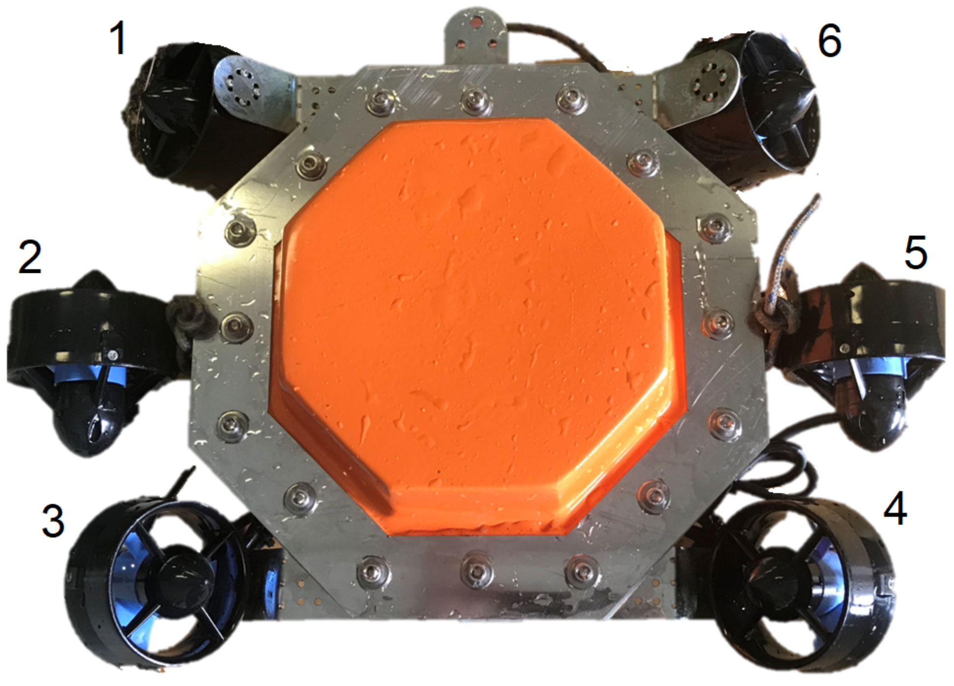
To demonstrate the applicability of Algorithm 1 we propose two numerical examples. They relate to the problem of PM organization for the unmanned underwater vehicle (UUV), which was considered in [6], regarding the criterion of maximizing the availability factor. The UUV (Figure 1) is the main part of an automated system for remote monitoring of underwater sections of a gas pipeline.

The UUV carries out a set of measures to externally inspect the offshore section of the gas pipeline, in order to determine its technical condition, to detect defects, and to provide data for subsequent analysis of the causes of defects. The UUV can move using six motors (1–6 in the Figure 1), and, depending on the type of installed engines, different situations for system failure are possible:

• The system failure occurs when any four motors fail regardless of their location. This situation is modeled as a 4-out-of-6: F-system and is presented in Section 4.2;
• The system failure depends on the location of its failed units, and occurs when three motors from one side and one motor from the other side fail (this situation will be denoted as $3+1$-out-of-6: F system), but the system does not fail when two motors fail on one side, and two motors on the other. Any next unit failure leads to the system failure (this situation will be denoted as a 5-out-of-6: F system).

Therefore, from the point of view of mathematical modeling, the last situation can be considered as a combination of the above two special types of k-out-of-$n:F$ systems, where failure depends on the position of its failed components. For such kind of systems, a special notation $(3+1,5)$-out-of-$6:F$ system is proposed and it is considered in Section 4.4. This model is the starting point of our numerical study. Since the initial information is very limited, we focus on the analysis of the sensitivity of decision making to the shape of the distribution of system unit lifetime.

To do this, we consider four types of popular distributions: (i) exponential, $Exp(\alpha$); (ii) Gamma distribution, $\mathrm{\Gamma }(\mathrm{\Theta },k)$; (iii) Gnedenko–Weibull distribution, $GW(\lambda ,k)$; (iv) log-normal distribution $LN(\mu ,{\sigma }^2)$. The parameters of all distributions in the experiments are chosen so that their expectations remain constant and coincide for all of these different distributions, being equal to 1, $a=\mathbf{E}\left[A_i\right]=1$. This means that we scaled the time with respect to the mean unit lifetime a. At that, the second parameters are chosen so that the coefficient of variation $v=\frac{\sigma }{a}$ varies in the interval $v\in [0.3,5.0]$. Analogously we choose the pricing scale in such a way that the reward equals to one, i.e., $c=1$.

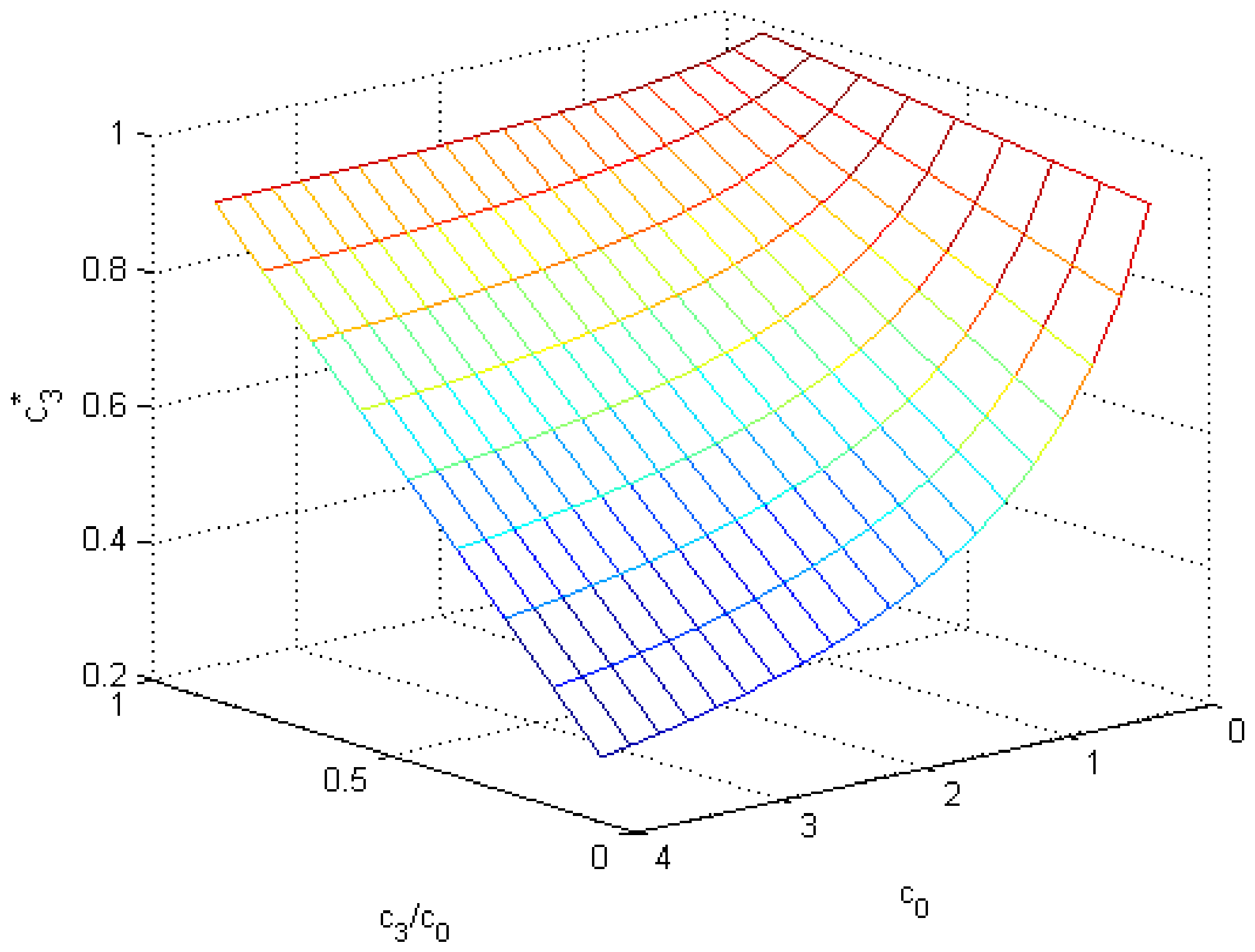
Let us see how change of the parameters $c_0,c_l$ affects the value $c_l^{*}.$ Due to representation of $c_l^{*}$ by (14), it is clear that in any case $c_l^{*}\le 1$. Moreover, if $c>>max\{c_0,c_l\}$, then $c_l^{*}\approx 1$. On the contrary, if c is negligible relative to the values $c_0$ and $c_l$, then $c_l^{*}\approx \frac{c_l}{c_0}$. For further numerical analysis, the parameter $c_3^{*}$ is essential and it is shown in Figure 2 with respect to the value $c_0$ and the ratio $\frac{c_3}{c_0}$.

Algorithm 1 was implemented as a MATLAB program code. The results of numerical experiments are presented as graphs plotted by the developed program.

4.2. PM of a System, Whose Failure Does Not Depend on the Location of Its Failed Units

First, consider a 4-out-of-$6:F$–system, where failure does not depend on the configuration of its failed units. In this case, only four strategies of PM control are possible:

• 0-strategy is that the system operates up to its failure;
• l-strategy ($l=$ 1, 2, 3) is to begin the PM when the system reaches the state l.

For our numerical experiment, we restrict ourselves to comparing the 0-strategy and 3-strategy. In this case, it is true that $E_3=\left\{3\right\}$ and $E_0=\left\{4\right\}$. The analytical expressions for the mean values $M_l$ are not always accessible. However, their numerical calculation in accordance, with Algorithm 1, is not too difficult and it is proposed below.

In this case, the general Algorithm 1 is essentially simplified, since the time to the subset $E_l$ destination coincides with respective ordered statistics $A_{\left(l\right)}$ of the times to the system unit failures $A_i:(i=\overline{1,6})$.

Therefore, Steps 1 and 3 of Algorithm 1 look like

Step 1.$E_3=\left\{3\right\},E_0=\left\{4\right\}$

Step 3.$F_3\left(t\right)=A_{\left(3\right)}\left(t\right),F_0\left(t\right)=A_{\left(4\right)}\left(t\right).$

All other steps remain unchanged.

The results of the calculations performed in accordance to the above procedure are presented in the following graphs. Figure 3 represents 3D graphs of surface $m_3^{*}$ for two values of $b_0$ versus variation coefficient v and fraction $\frac{b_3}{b_0}$ jointly with their level curves for different values of $c_3^{*}$.

The upper graphs show the surfaces $m_3^{*}$ for the Gamma distribution of the system unit lifetime for the values $b_0=0.001$ (left) and $b_0=0.1$ (right) and their intersection with the plane corresponding to the value of the indicator $c_3^{*}=0.7$. The red line on the surfaces corresponds to an exponential distribution, at which the surface turns into a curve. Above the plane, the 3-strategy gains an advantage over the 0-strategy. Below the plane, it is preferable to use the 0-strategy. As can be seen from the graphs, for the exponential distribution of the system units lifetime, the 3-strategy will be preferable over 0-strategy, regardless of the $\frac{b_3}{b_0}$ ratio. For the Gamma distribution, the decision on the choice of the PM strategy depends on the value of the $\frac{b_3}{b_0}$ ratio and the coefficient of variation v.

The lower graphs show the level curves of the $m_3^{*}$-surface for different values of $c_3^{*}$ for four types of distributions: $\mathrm{\Gamma }(\mathrm{\Theta },k)$ (solid curves), $GW(\lambda ,k)$; (dashed curves), $LN(\mu ,{\sigma }^2)$ (dotted curves), and Exp($\alpha$) (red circle), where the axis labels correspond to the upper graph. Above the level curve, preference should be given to the 3-strategy, below—to the 0-strategy.

The red circle on the solid magneto color line corresponds to the exponential distribution of the system unit lifetime at the value of the cost criterion $c_3^{*}=0.9$. In that case, for an exponential distribution, the value of the $\frac{b_3}{b_0}$ ratio will influence the decision on choosing the best strategy.

The results can be used as a DM adviser and demonstrate the possibility of studying the sensitivity of the decision about PM to the type of distribution of the lifetime of the system units.

4.3. Special Case: PM of a K-Out-Of-n: F–System, for Exponential Distributions of Unit Lifetimes

Under the assumption about exponential distributions of the lifetimes of the system units $A_i$, $A\left(t\right)=\mathbf{P}\{A_i\le x\}=1-e^{-\alpha t}$, the analytical calculation of the parameter $m^{*}$ is possible for any k and n. The distributions of ordered statistics can be calculated as sums of the intervals $T_i=A_{\left(i\right)}-A_{(i-1)}$ between them. Thus,

$$S_{\left(l\right)}=T_1+\cdots +T_l.$$

(22)

Due to the independence of the residual lifetimes of all non-failed units on the failure time of any of them, the intervals $T_i$ are

$$T_i=min\{A_1,A_2,\dots A_{n-(i-1)}\}.$$

(23)

Therefore, they are independent, exponentially distributed r.v.s with parameters ${\lambda }_i=(n-i+1)\alpha .$ Hence,

$$F_i\left(t\right)=\mathbf{P}\{T_i\le t\}=1-\mathbf{P}\{T_i>t\}=1-{(1-A\left(x\right))}^{n-i}=1-e^{(n-(i-1\left)\right)\alpha t}.$$

(24)

Thus, $\mathbf{E}\left[T_i\right]={\left[(n-(i-1))\alpha \right]}^{-1}$ and, therefore, for the special case $n=6,k=4$, it holds

$$M_l=\mathbf{E}{S}_l=\mathbf{E}{T}_1+\cdots +T_l=\frac{1}{6\alpha }+\cdots +\frac{1}{(6-(l-1\left)\right)\alpha }.$$

(25)

In particular, $M_3=\frac{37}{60\alpha },M_0=M_4=\frac{57}{60\alpha }.$ Taking into account this and the fact that $\alpha =1$, we obtain an analytical expression for the red curves in the upper graphs in Figure 3 as a function of $m_3^{*}$ versus $\frac{b_3}{b_0}$

$$m_3^{*}=\frac{m_3+1}{m_0+1}=\frac{b_0(M_3+b_3)}{b_3(M_0+b_0)}=\frac{1}{\frac{b_3}{b_0}}·\frac{\frac{M_3}{b_0}+\frac{b_3}{b_0}}{\frac{M_0}{b_0}+1}.$$

(26)

Therefore, according to the necessary and sufficient condition (15), the 3-strategy will be preferable to the 0-strategy, if

• $m_3^{*}=\frac{37+0.06\frac{b_3}{b_0}}{57.06\frac{b_3}{b_0}}>c_3^{*},$ for $b_0=0.001$,
• $m_3^{*}=\frac{37+6\frac{b_3}{b_0}}{63\frac{b_3}{b_0}}>c_3^{*},$ for $b_0=0.1$.

Following the equation $m_3^{*}=c_3^{*}=0.9$, one can calculate $\frac{b_3}{b_0}\approx 0.7213$ for $b_0=0.001$ and $\frac{b_3}{b_0}\approx 0.7298$ for $b_0=0.1$. These values coincide with the coordinates of the red circles shown in Figure 3.

4.4. PM of a System, Whose Failure Depends on the Location of the Failed Units

If the system failure depends on the location of the failed units, the comparison of strategies and the decisions about the choice of PM are system-specific and depend on the exploitation conditions. In this case, we consider the model described in Section 4.1 and presented in Figure 1, which is denoted as the $(3+1,5)$-out-of-$6:F$ system.

Further, for convenience, a binary code is used to indicate system states, namely the number of the state $\mathbf{j}=(j_1,j_2,\cdots j_6)$ is given in accordance to the formula

$$j=\left|\mathbf{j}\right|=\sum _{0\le i\le 6}{j}_i{2}^{6-i}.$$

(27)

Then, the set of failure states $E_0$ consists of a combination of states with four failures and five failures.

By analogy with Section 4.2, we consider two strategies:

• 0-strategy: run up to the system failure. The subset of the states for the repair beginning is $E_0$;
• 3-strategy: start the PM after the failure of any three units. The subset of the states for the PM beginning is $E_3$.

In this case the ordered statistics do not uniquely determine the time to the corresponding subset of state $E_0$ destination. Thus, to apply Algorithm 1, it is necessary to specify some of its steps.

• Step 1. To form a set of repair start states, consider the set of states with four failed units,

  $$E_4=\{15,23,27,29,30,39,43,45,46,51,53,54,57,58,60\}.$$

  (28)
  In this set, the red states are associated with three failed units on one side and one ion other side, denoted as $(3+1)$, when the system failure occurs. The blue states are associated with two units failed one one side and two on the other, denoted as $(2+2)$, which leads to the system failure after any next unit failure.
  The three-strategy starts after the failure of any three units, the subset for it is $E_3$.
• Step 2. Accordingly to step 1, the times $S_0$ for the system failure coincide with ordered statistics $A_{\left(4\right)}$ for red states of subset $E_4$, and coincide with ordered statistics $A_{\left(5\right)}$ for blue states of subset $E_4$.

  $$S_0=\left\{\begin{array}{c}{A}_{\left(4\right)},\mathrm{if}\mathrm{the}\mathrm{system}\mathrm{is}\mathrm{in}“\mathrm{red}”\mathrm{state}{E}_4,\hfill \\ A_{\left(5\right)},\mathrm{if}\mathrm{the}\mathrm{system}\mathrm{is}\mathrm{in}“\mathrm{blue}”\mathrm{state}{E}_4,\hfill \end{array}\right.$$

  (29)
  The time $S_3$ to the set $E_3$ destination coincide with the relevant ordered statistics namely: $S_3=A_{\left(3\right)}.$
• Step 3. Does not change. The distributions $A_{\left(j\right)}\left(t\right)$ of the j-th ordered statistics are calculated according to (20),

  $$A_{\left(j\right)}\left(x\right)=\mathbf{P}\{X_{\left(j\right)}\le x\}=\sum _{j\le i\le n}\left(\genfrac{}{}{0pt}{}{n}{i}\right)A^i\left(x\right){(1-A\left(x\right))}^{n-i}.$$

  (30)
• Step 4. The distribution of the time $S_0$ to the subset $E_0$ destination according to its determination by (29) equals to

  $$F_0\left(t\right)=\frac{6}{15}{A}_{\left(4\right)}\left(t\right)+\frac{9}{15}{A}_{\left(5\right)}\left(t\right)=\frac{2}{5}{A}_{\left(4\right)}\left(t\right)+\frac{3}{5}{A}_{\left(5\right)}\left(t\right).$$
  The distribution of the subset of states $E_3$ destination is $F_3\left(t\right)=A_{\left(3\right)}\left(t\right).$ Appropriate expectations of times to the subsets $E_l$ for $l=0$ and $l=3$ destinations are

  $$M_0=\frac{2}{5}\mathbf{E}\left[A_{\left(4\right)}\right]+\frac{3}{5}\mathbf{E}\left[A_{\left(5\right)}\right],M_3=\mathbf{E}\left[A_{\left(3\right)}\right].$$
• Step 5. Does not change: following to step 5 of the Algorithm 1, calculate $m_0,m_3,m_3^{*}$.
• Step 6. Compare the calculated values $m_3^{*}$ with indicator $c_3^{*}$, according to the rule given by (15) as advice to a DM in order to choose the best strategy.
• Stop.

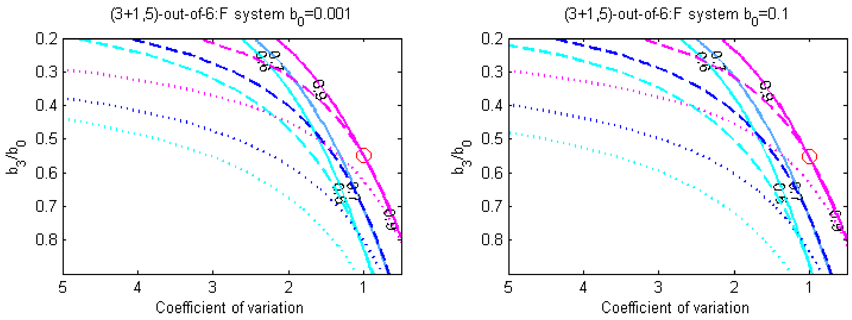
The results of the numerical experiments are presented in Figure 4.

The graphs show the level curves of the surface $m_3^{*}$ for the values $b_0=0.001$ (on the left) and $b_0=0.1$ (on the right). The color of curves corresponds to the values of the cost criterion $c_3^{*}$: 0.6 (cyan), 0.7 (blue), 0.9(magneto). The graphs show the results for four different distributions of system unit lifetimes: $\mathrm{\Gamma }(\mathrm{\Theta },k)$ (solid curves), $GW(\lambda ,k)$ (dashed curves), $LN(\mu ,{\sigma }^2)$ (dotted curves), and $Exp(\alpha$), where the axis labels correspond to Figure 3.

In contrast to the model, whose failure does not depend on position of its failed units, the influence of the parameter $b_0$ is much less (especially for a gamma distribution), in comparison to the ratio $\frac{b_3}{b_0}$. The shape of the lifetime distribution, as well as the coefficient of variation v, have a particular influence on the choice of the preferred strategy. Compared to the previous case, the area where the 0-strategy is preferable, has increased significantly. Both considered cases show that, for making decisions on the choice of the best PM strategy, it is not enough to take into account only the expectation of system unit lifetimes and the costs of PM and repair.

4.5. Special Case: PM of a $(3+1,5)$-Out-Of-6$:F$ – System for Exponential Distribution of Unit Lifetimes

In the special case of exponential distribution of system unit lifetimes, it is possible to use the same approach as in Section 4.3 and the problem can be solved analytically.

In this case, as before, it holds $M_3=\frac{37}{60\alpha },M_4=\frac{57}{60\alpha }$ and therefore $M_5=M_4+\frac{1}{2\alpha }=\frac{87}{60\alpha }$. From here, it follows

$$M_0=\frac{2}{5}\mathbf{E}\left[A_{\left(4\right)}\right]+\frac{3}{5}\mathbf{E}\left[A_{\left(5\right)}\right]=\frac{2}{5}{M}_4+\frac{3}{5}{M}_5=\frac{375}{300\alpha }=\frac{5}{4\alpha }.$$

(31)

Substitution of the calculated $M_3$ and $M_0$ for the exponential distribution makes it possible to obtain $m_3^{*}$ as a function of $\frac{b_3}{b_0}$ and to formulate a necessary and sufficient condition (15) for the 3-strategy preference over the 0-strategy for this system, in the case $b_0=0.001$, in the form

• $m_3^{*}=\frac{37+0.06\frac{b_3}{b_0}}{75.06\frac{b_3}{b_0}}>c_3^{*},$
  and in the case $b_0=0.1$ as
• $m_3^{*}=\frac{37+6\frac{b_3}{b_0}}{81\frac{b_3}{b_0}}>c_3^{*}.$

The coordinates of the red circles presented in Figure 4 for $c_3^{*}=0.9$ can be calculated analytically: $\frac{b_3}{b_0}\approx 0.5482$ for $b_0=0.001$ (Figure 4, graph on the left) and $\frac{b_3}{b_0}\approx 0.5531$ for $b_0=0.1$ (Figure 4, graph on the right). These results are in complete agreement with the numerical calculations.

5. Conclusion

The paper deals with the choice of a preferable PM strategy for the k-out-of-n system to maximize the long run average system reward. The PM strategies are based on the system state observations. Ordered statistics are used as indicators for PM and repair start times.

The general conditions for the comparison of any PM strategy were obtained and an algorithm for their application was developed. The obtained theoretical results and the algorithm allow investigating the sensitivity of the decision making in regard to the shape of the system unit lifetime distributions. The algorithm was implemented for two examples arising from some real word problems. For the special case of exponential distribution of system unit lifetimes, explicit analytical results were obtained. The results of numerical calculations coincide with those from the analytical study. A series of numerical experiments shows the sensitivity of a PM strategy choice in regard to the shape of the system unit lifetime distributions.

The novelty and features of this study are:

• A method for PM investigations of k-out-of-n: F systems, whose failures depend on the positions of failed units developed;
• A new approach based on ordered statistics if used to solve the problem;
• A cost-type criterion for PM strategies comparison is used;
• A study of the sensitivity of decision making to the shape of system unit lifetime distributions is carried out.

References

- Trivedi, K. Probability and Statistics with Reliability, Queuing and Computer Science Applications, 2nd ed.; John Wiley & Sons: New York, NY, USA, 2016. [Google Scholar]
- Chakravarthy, S.; Krishnamoorthy, A.; Ushakumari, P. A k-out-of-n reliability system with an unreliable server and Phase type repairs and services: The (N,T) policy. J. Appl. Math. Stoch. Anal. 2001, 14, 361–380. [Google Scholar] [CrossRef] [Green Version]
- Rykov, V.; Kozyrev, D.; Filimonov, A.; Ivanova, N. On reliability function of a k-out-of-n system with general repair time distribution. Probab. Eng. Inform. Sci. 2020, 35, 885–902. [Google Scholar] [CrossRef]
- Pascual-Ortigosa, P.; Sáenz-de-Cabezón, E. Algebraic Analysis of Variants of Multi-State k-out-of-n Systems. Mathematics 2021, 9, 2042. [Google Scholar] [CrossRef]
- Rykov, V.; Sukharev, M.; Itkin, V. Investigations of the Potential Application of k-out-of-n Systems in Oil and Gas Industry Objects. J. Mar. Sci. Eng. 2020, 8, 928. [Google Scholar] [CrossRef]
- Rykov, V.; Kochueva, O.; Farkhadov, M. Preventive Maintenance of a k-out-of-n System with Applications in Subsea Pipeline Monitoring. J. Mar. Sci. Eng. 2021, 9, 85. [Google Scholar] [CrossRef]
- Vishnevsky, V.; Kozyrev, D.; Rykov, V.; Nguen, Z. Reliability modeling of the rotary-wing flight module of a high-altitude telecommunications platform. Inform. Technol. Comput. Syst. 2020, 4, 26–38. (In Russian) [Google Scholar]
- Shiryaev, A.N. Some new results in theory of controllable random processes. In Trans. Fourth Prague Conf. on Information Theory, Statistical Decision Functions, Random Processes, Prague, Czech Republic, 1965; Academia: Prague, Czech Republic, 1965; pp. 131–203. [Google Scholar]
- Boucherie, R.; vanDijk, N. Markov Decision Processes in Practice; Springer International Publishing: Cham, Switzerland, 2017. [Google Scholar]
- Howard, R. Dynamic Programming and Markov Processes; John Wiley & Sons: New York, NY, USA, 1960. [Google Scholar]
- Wolfe, P.; Dantzig, G. Linear Programming in a Markov Chain. Oper. Res. 1962, 10, 702–710. [Google Scholar] [CrossRef]
- Puterman, M. Markov Decision Processes. In Handbooks in Operations Research and Management Science; Heyman, D., Sobel, M., Eds.; Elsevier: Amsterdam, The Netherlands, 1990; Volume 2, pp. 331–434. [Google Scholar]
- Rykov, V. Controllable Queueing Systems. Itogi Nauk. Tech. Probab. Theory. Math. Stat. Theor. Cybern. 1975, 12, 143–153. (In Russian) [Google Scholar]
- Rykov, V. Controllable Queueing Systems: From the Very Beginning up to Nowadays. Reliab. Theory Appl. 2017, 12, 39–61. [Google Scholar]
- Kitaev, V.; Rykov, V. Controlled queueing systems. Int. J. Stoch. Anal. 1995, 8, 433–435. [Google Scholar]
- Hernandez-Lerma, O.; Lasssrerre, J. Discrete time Markov Control Processes Basic Optimality Criteria; Springer: New York, NY, USA, 1996. [Google Scholar]
- Sennott, L. Stochastic Dynamic Programming and the Control of Queueing Systems; Wiley-Interscience: Hoboken, NJ, USA, 1999. [Google Scholar]
- Gertsbakh, I. Reliability Theory with Applications to Preventive Maintenance; Springer: Berlin/Heidelberg, Germany, 2000. [Google Scholar]
- Dudin, A.; Krishnamoorthy, A.; Viswanath, C. Reliability of a k-out-of-n-system through Retrial Queues. In Proceedings of the Trans. of XXIV International Seminar on Stability Problems for Stochastic Models, Jurmala, Latvia, 10–17 September 2004. [Google Scholar]
- Krishnamoorthy, A.; Viswanath, C.N.; Deepak, T.G. Reliability of a k-out-of-n-system with Repair by a Service Station Attending a Queue with Postponed Work. Int. J. Reliab. Qual. Saf. Eng. 2007, 14, 379–398. [Google Scholar] [CrossRef]
- Krishnamoorthy, A.; Viswanath, C.N.; Deepak, T.G. Maximizing of Reliability of a k-out-of-n-system with Repair by a facility attending external customers in a Retrial Queue. Reliab. Theory Appl. 2007, 2, 21–33. [Google Scholar]
- Krishnamoorthy, A.; Sathian, M.K.; Viswanath, C.N. Reliability of a k-out-of-n system with repair by a single server extending service external customers with pre-emption. Reliab. Theory Appl. 2016, 11, 61–93. [Google Scholar]
- Krishnamoorthy, A.; Sathian, M.K.; Viswanath, C.N. Reliability of a k-out-of-n system with a single server extending non-preemptive service to external customers-Part I. Reliab. Theory Appl. 2016, 11, 62–75. [Google Scholar]
- Krishnamoorthy, A.; Sathian, M.K.; Viswanath, C.N. Reliability of a k-out-of-n system with a single server extending non-preemptive service to external customers-Part II. Reliab. Theory Appl. 2016, 11, 76–88. [Google Scholar]
- Pham, H.; Wang, H. Optimal opportunistic maintenance of a k-out-of-n:G system. Int. J. Reliab. Qual. Saf. Eng. 1997, 4, 369–386. [Google Scholar]
- Pham, H.; Wang, H. Optimal (τ, T) Opportunistic Maintenance of a k-out-of-n:G System with Imperfect PM and Partial Failure. Nav. Res. Logist. 2000, 47, 223–239. [Google Scholar] [CrossRef]
- Geng, J.; Azarian, M.; Pecht, M. Opportunistic maintenance for multi-component systems considering structural dependence and economic dependence. J. Syst. Eng. Electron. 2015, 26, 493–501. [Google Scholar] [CrossRef]
- Finkelstein, M.; Levitin, G. Preventive maintenance for homogeneous and heterogeneous systems. Appl. Stoch. Model. Bus. Ind. 2019, 35, 908–920. [Google Scholar] [CrossRef]
- Finkelstein, M.; Cha, J.H.; Levitin, G. On a new age-replacement policy for items with observed stochastic degradation. Qual. Reliab. Eng. Int. 2020, 36, 1132–1146. [Google Scholar] [CrossRef]
- Park, M.; Lee, J.; Kim, S. An optimal maintenance policy for k-out-of-n system without monitoring component. Qual. Technol. Qual. Manag. 2019, 16, 140–153. [Google Scholar] [CrossRef]
- Endharth, A.J.; Yun, W.Y.; Yamomoto, H. Preventive maintenance policy for linear-consecutive -k-out-of-n:F system. J. Oper. Res. Soc. Jpn. 2016, 59, 334–346. [Google Scholar]
- Hamdan, K.; Tavangar, M.; Asadi, M. Optimal preventive maintenance for repairable weighted k-out-of-n systems. Reliab. Eng. Syst. Safe 2021, 205, 107267. [Google Scholar] [CrossRef]
- Jonge, B.D.; Scarf, P.A. A review on maintenance optimization. Eur. J. Oper. Res. 2020, 285, 805–824. [Google Scholar] [CrossRef]
- Rykov, V. On Reliability of Renewable Systems. In Reliability Engineering. Theory and Applications; Vonta, I., Ram, M., Eds.; CRC Press: Boca Raton, FL, USA, 2018; pp. 173–196. [Google Scholar]
- Rykov, V. Decomposable semi-regenerative processes: Review of theory and applications to queueing and reliability systems. Reliab. Theory Appl. 2021, 16, 157–190. [Google Scholar]
- Klimov, G. An Ergodic Theorem for Regenerating Processes. Theory Probab. Its Appl. 1976, 21, 392–395. [Google Scholar] [CrossRef]
Figure 1.
The unmanned underwater vehicle.
Figure 2.
The cost criterion versus and the ratio .
Figure 3.
The surfaces for and versus coefficient of variation v and fraction (upper graphs) and level curves of the surface (lower graphs) for the 4-out-of-–system.
Figure 4.
Level curves for versus variation coefficient v and fraction for -out-of-6 – system.
Publisher’s Note: MDPI stays neutral with regard to jurisdictional claims in published maps and institutional affiliations. |
© 2021 by the authors. Licensee MDPI, Basel, Switzerland. This article is an open access article distributed under the terms and conditions of the Creative Commons Attribution (CC BY) license (https://creativecommons.org/licenses/by/4.0/).
Share and Cite
MDPI and ACS Style
Rykov, V.; Kochueva, O.; Rykov, Y. Preventive Maintenance of the k-out-of-n System with Respect to Cost-Type Criterion. Mathematics 2021, 9, 2798. https://0-doi-org.brum.beds.ac.uk/10.3390/math9212798
AMA Style
Rykov V, Kochueva O, Rykov Y. Preventive Maintenance of the k-out-of-n System with Respect to Cost-Type Criterion. Mathematics. 2021; 9(21):2798. https://0-doi-org.brum.beds.ac.uk/10.3390/math9212798
Chicago/Turabian StyleRykov, Vladimir, Olga Kochueva, and Yaroslav Rykov. 2021. "Preventive Maintenance of the k-out-of-n System with Respect to Cost-Type Criterion" Mathematics 9, no. 21: 2798. https://0-doi-org.brum.beds.ac.uk/10.3390/math9212798
Note that from the first issue of 2016, this journal uses article numbers instead of page numbers. See further details here.