Interactive Scientific Visualization of Fluid Flow Simulation Data Using AR Technology-Open-Source Library OpenVisFlow

Abstract

Computational fluid dynamics (CFD) are being used more and more in the industry to understand and optimize processes such as fluid flows. At the same time, tools such as augmented reality (AR) are becoming increasingly important with the realization of Industry 5.0 to make data and processes more tangible. Placing the two together paves the way for a new method of active learning and also for an interesting and engaging way of presenting industry processes. It also enables students to reinforce their understanding of the fundamental concepts of fluid dynamics in an interactive way. However, this is not really being utilized yet. For this reason, in this paper, we aim to combine these two powerful tools. Furthermore, we present the framework of a modular open-source library for scientific visualization of fluid flow “OpenVisFlow” which simplifies the creation of such applications and enables seamless visualization without other software by allowing users to integrate the visualization step into the simulation code. Using this framework and the open-source extension AR-Core, we show how a new markerless visualization tool can be implemented.

1. Introduction

Computational fluid dynamics (CFD) is a very useful tool to understand and optimize complex processes and machines. It is widely used in industries such as automotive [1], aerospace [2], and chemical engineering. Thus, the simulation results serve as a basis for decision-making. Since CFD is already part of the everyday life of an engineer, this tool is being taught to students as standard during studies. However, building and understanding resulting simulation data can be very time-consuming, and additional tools such as Paraview or Gnuplot are needed to bring the results into a suitable and presentable form. Depending on the discipline, this can be a problem for teaching, as students can lose their concentration over time [3]. This in turn leads to a worsened learning experience. It can be helpful if the simulation results are visualized in advance or just in time, so that students can better interact with them.

In the past few years, there has been a strong growth in the demand for augmented reality (AR) and virtual reality (VR) applications, as Mojtaba Noghabaei et al. [4] show in their work, taking into account extensive surveys. AR in particular is increasingly used in areas such as medicine, mechanical engineering, and process engineering. Even for the medical field, especially for surgery, it can be a powerful tool to provide additional information to the surgeon, as shown in the work by Raabid Hussain et al. [5]. In the work by Anna V. Iatsyshyn et al. [6], they analyze in detail the usability in the modern era. They show that AR has a significant value for teaching. Furthermore, they explain that there are currently not many experts in this field and that future experts should be trained for the new technological era. While there are already specific applications that combine CFD with AR, there is not yet one that provides an interface to easily visualize any simulation.

Several AR applications are already available that are geared toward the teaching field, and many areas benefit from these. The application cleARmath [7] can visualize vector geometries in AR and thus provide a playful learning experience as well as a better understanding of the position of planes, vectors, etc. TeachAR [8] is an application that allows non-English speakers to playfully learn colors, 3D shapes, and spatial relations in English. The BARETA [9] application is designed to provide medical students with a better understanding of where the ventricular system is located in the brain. Evaluations were carried out for each of the applications mentioned. The majority of the persons tested were able to derive a benefit from the respective application. Based on this information, an application that visualizes complex processes such as fluid flow in AR would be a viable tool to better understand them. There are already AR applications with respect to computational fluid dynamics (CFD). In their work, Jia-Rui Lin et al. [10] visualized the thermal environment that occurs indoors in AR. They developed their own file format (cfd14a) which can be accessed via a server on the smartphone. There are several papers dealing with the visualization of CFD simulations [11,12,13,14,15].

Serkan Solmaz and Tom Van Gerven [16] describe in their work that CFD simulations are difficult to understand for non-experts, which limits their use. They present a method using Unity with the Vuforia extension to retrieve CFD simulations from a server and display them in AR. In our work, we take a different approach. We do not use the closed-source extension Vuforia, but the open-source variant Google AR Core. With this, we are able to develop an open-source modular library. The goal is to create an interface between powerful tools such as CFD and AR visualization that can be used by developers to create applications that can visualize complex processes. Furthermore, the main goal of the library is to fully integrate visualization into the simulation itself to allow users to visualize the mentioned processes on a cluster and stream the results in real time. Such a feature would enable interesting training and testing applications in a variety of domains. In this paper, we present the framework for such a library, which allows us to embed computed transport fields into 3D objects. In addition, the library allows the developer to choose from different visualization methods. One of these methods is the markerless geometry overlay that we developed, which is also presented in this paper. Since the ARCore extension is open source, everything can be customized to the user’s personal needs. Extensions such as Vuforia do not allow this because they are closed source. This enables research into new visualization approaches, as shown in this paper with the novel markerless geometry overlay.

The contributions in our paper can be summarized as follows: Development of an application OpenLBar with updateable simulations; a method of geometry overlay without using a neural network; introducing an open-source library for AR application development. The resulting framework allows an easy extension of visualization methods and offers the possibility to fully integrate simulations into the code.

In the remainder of the paper, we first present the basic concept of our project. Then, the functionalities of the application and the open-source library are presented in the realization part using the example application OpenLBar. Finally, the advantages of visualizing simulations in AR are quantitatively and qualitatively reviewed.

2. Concept

The main aim is a scientific visualization concept that allows CFD data to be experienced with AR/VR and provides an interface between simulation and visualization software. Creating a direct link between the two allows for the direct visualization and subsequent streaming from the cluster as well as an option to integrate changes made in VR back to the simulation on the cluster. In short, it would allow for the creation of a truly interactive simulation environment.

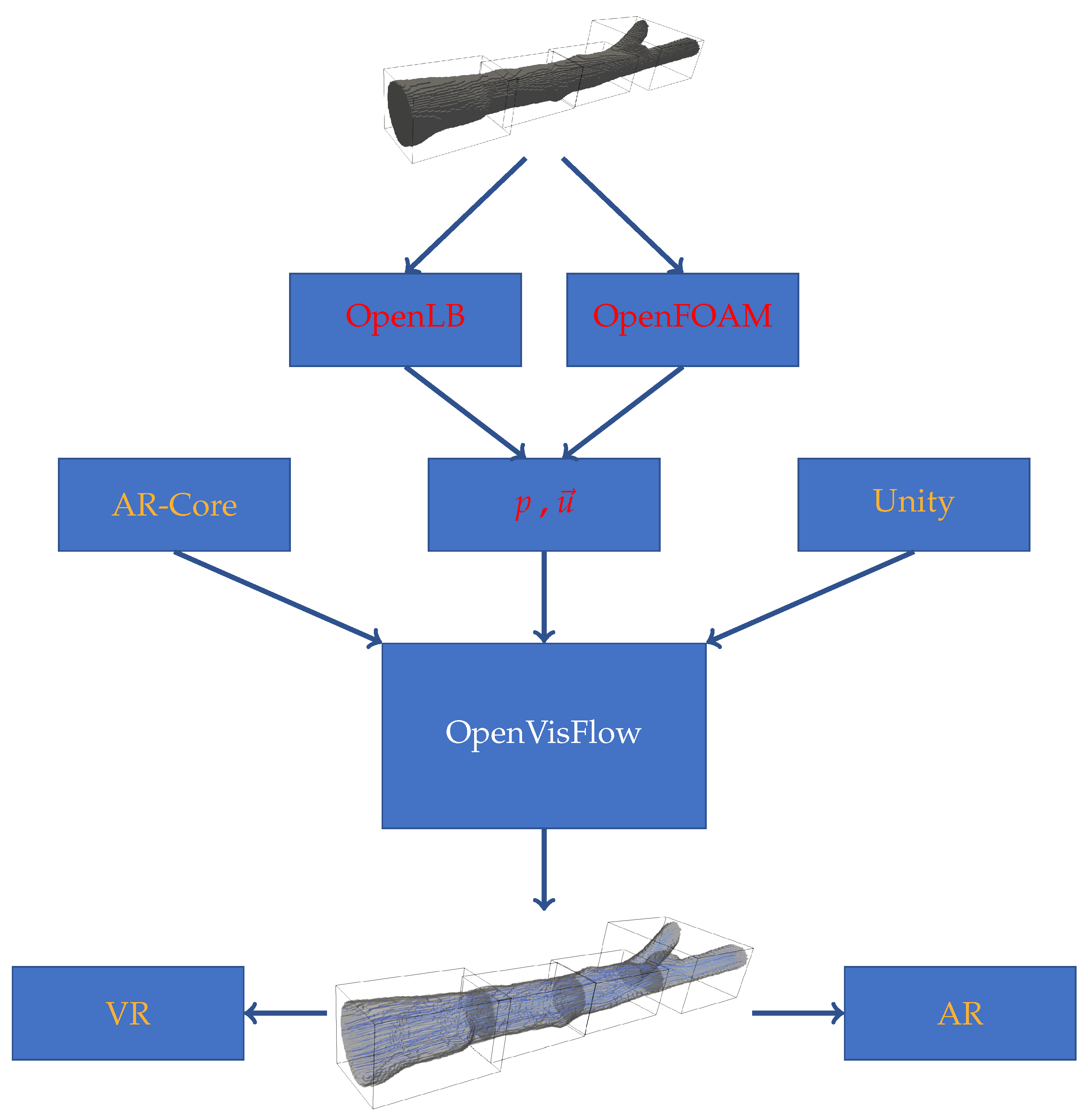
The visualization should be in different display modes such as screen, AR, and VR. As shown in Figure 1, it should also serve as a direct interface between simulation software and the visualization tool. With it, different applications, such as OpenLBar, which is presented in this paper, can be created. OpenLBar is the first result of this library.

In the CFD area, the Navier–Stokes equation (NSE) is of particular importance. For simplicity, we consider the simplified NSE for non-compressible fluids [17]. This is defined as

$$\frac{D\overrightarrow{u}}{Dt}=-\frac{\nabla p}{\rho }+\nu ·\Delta \overrightarrow{u}+\overrightarrow{F},$$

(1)

where $\frac{D}{Dt}=\frac{\delta }{{\delta }_t}+u·\nabla$ is the material derivative which indicates the temporal and spatial changes; $\rho$ is the density; $\Delta$ is the Laplace operator; $\nu$ is the kinematic viscosity; $\nabla p$ is the pressure gradient; $\overrightarrow{F}$ is the force vector; and $\overrightarrow{u}$ is the velocity vector. By solving this equation with the finite difference or lattice Boltzmann method (LBM), one then obtains the information about the pressures p and the velocities u. It should be noted that the LBM equations are not the same as the NSE, since they describe the mesoscopic level; however, the NSE can be recovered from LBM with the Chapman–Enskog analysis [18], although this will not be discussed further here, since it is not the focus of this work.

There are several ways to make the results obtained by the simulation software usable for the library. In the first, we access the simulation software directly with functions. However, this only works if the simulation is running in near real time. For this reason, this will be implemented at a later time. In the second solution, and thus the one pursued in this paper, ready-made simulations are provided externally. These are then to be displayed using different visualization techniques. To achieve this, an RES interface between web server and end device is implemented. For the development of our visualization methods, we access the functionalities of Unity and AR Core. To show the use of OpenVisFlow, an application named OpenLBar was created with it. This is intended to allow students to interact with simulations of fluid flows and thereby gain a better understanding of the complex processes involved.

3. Realization

In this section, we first discuss the method for providing the simulation data. For this, we use a server, as in [16], on which the data are stored ready for retrieval. What follows is the visualization of the CFD data on a QR code. Here, instead of the closed-source extension Vuforia, as in [16], the open-source variant Google ARCore is used. After that, the markerless geometry overlay is described. Since the making of 3D objects and the implementation of AR-Code can be a lengthy, drawn-out process, we propose and implement a framework for an open-source library in order to simplify and streamline the visualization process. As already stated in Section 2, the goal of this library is to bridge the present gap between simulation software and visualization. Currently, in order to visualize simulations, one must resort to separate programs such as Paraview. It is our goal to implement a library so that simulation and visualization can be implemented and executed at the same time to allow for a more optimized and efficient workflow, and eventually to allow for real-time physical simulations that are interactive. As can be seen from Figure 1, the library will use well-known and already tested simulation software such as OpenFOAM and OpenLB, take the results thereof, and visualize them using different tools and devices.

3.1. Providing the Simulation Data

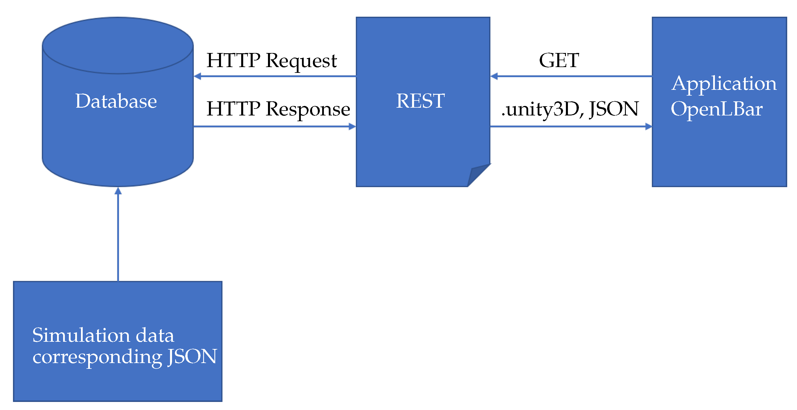
Creating simulation data and making them presentable can be very time-consuming and computationally intensive. Students or teaching staff usually do not always have the time and/or expertise to create these themselves. Furthermore, simulations can take up a significant amount of memory. Consequently, this has a strong impact on the use of the application for teaching. For this reason, the application OpenLBar allows the simulation data intended for teaching to be loaded onto the smartphone via a cloud, as shown in Figure 2. The data are provided by experts in the simulation field. Additionally, the user also has the option to store the simulation data locally or temporarily in the cache so that the storage space of the smartphone is not taken up by the transferred data. 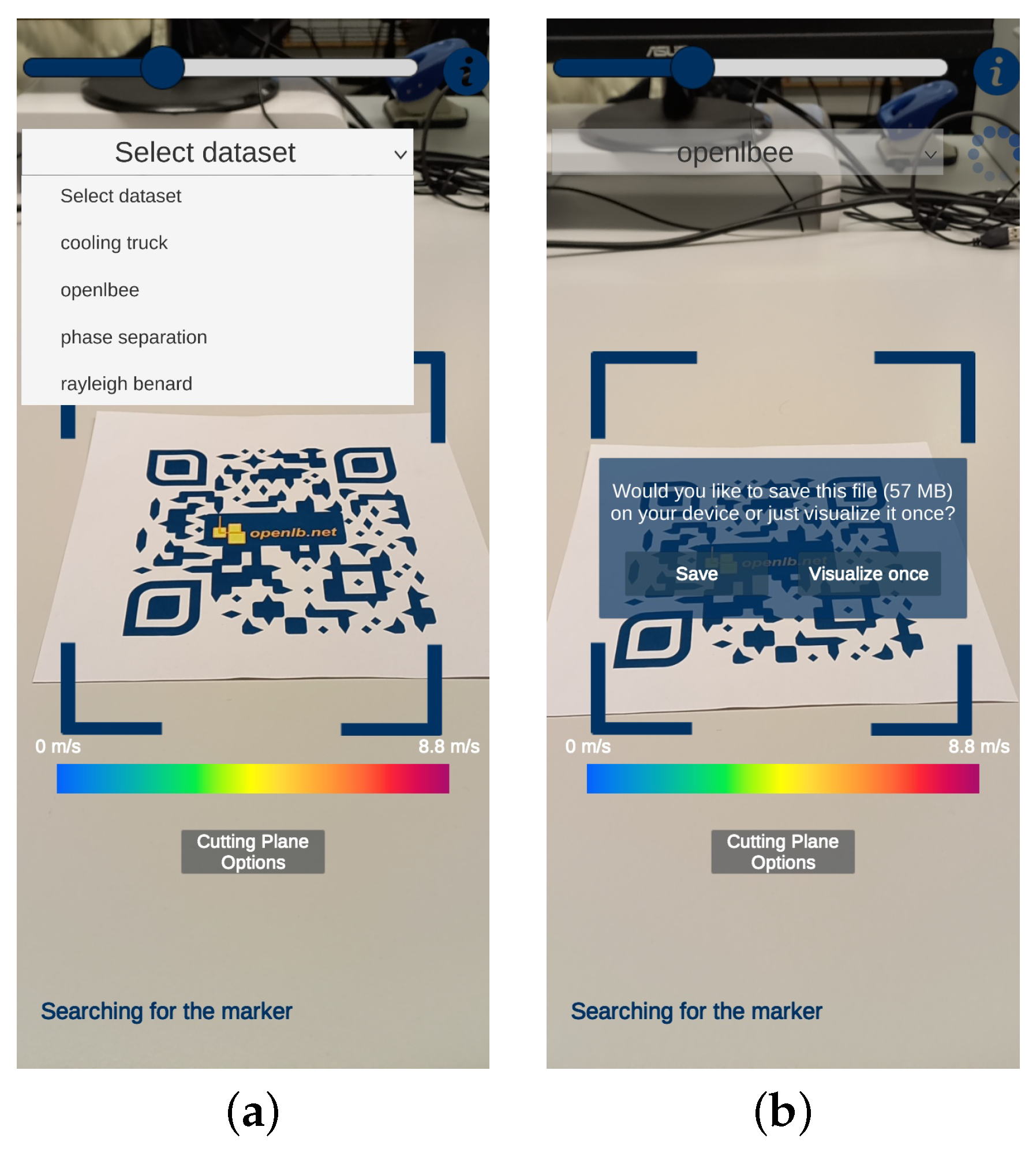Figure 3a shows that in the application, the simulations are selectable from a drop-down menu. The available data update with changes on the cloud and do not need to be synchronized manually. Figure 3b shows the user options after selecting the desired simulation.

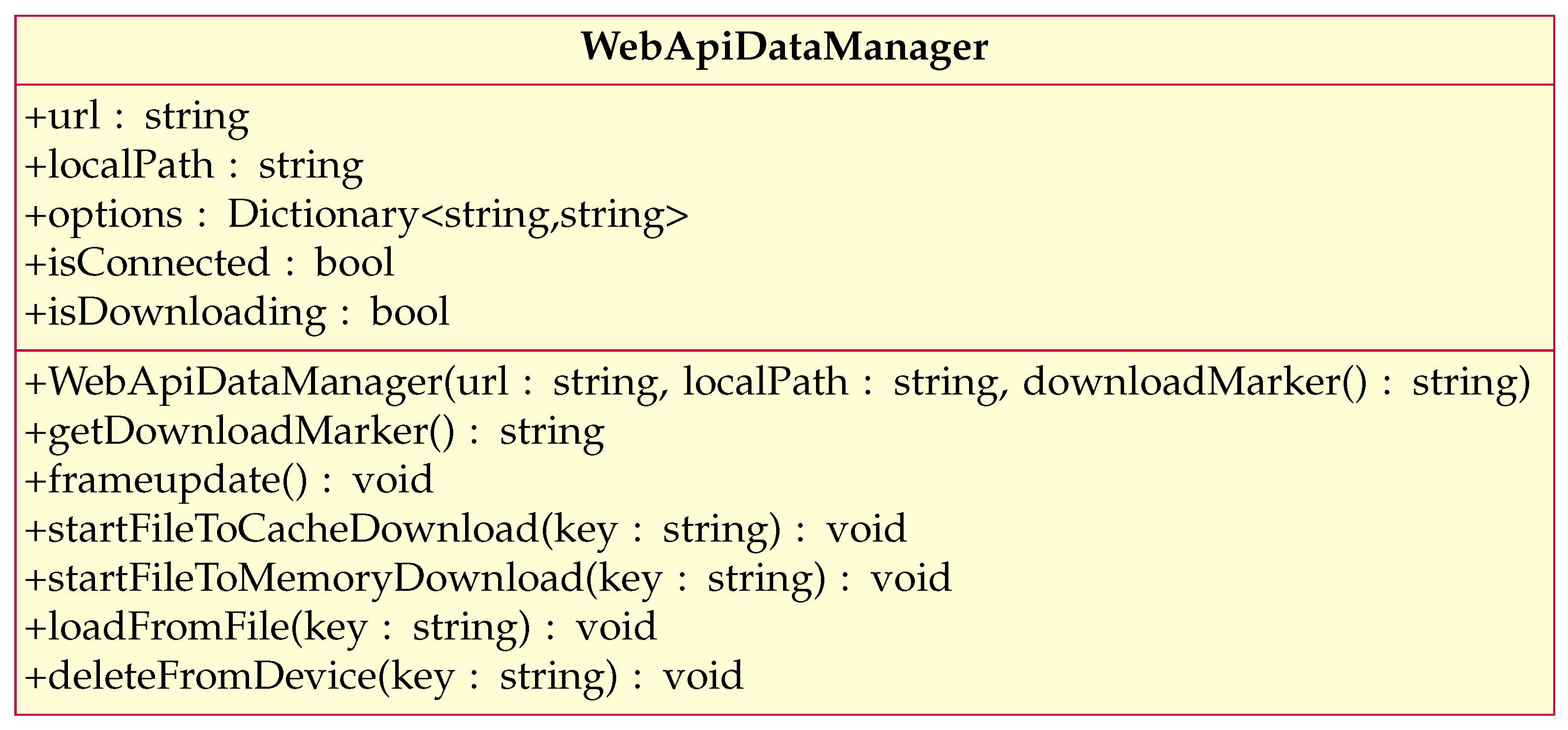
This functionality is realized through the WebApiDataManager of OpenVisFlow, which can be seen in Figure 4. When connected to a correct REST interface on a server, it will generate a list of accessible datasets which are then linked with a name through a dictionary, so that they can be displayed in a more user-friendly way. Using this, the name loading request can be started in three different ways. First, the dataset in question can be downloaded with the startFileToMemoryDownload function from the server onto the device, saving it on the local drive for later use. With the startFileToCacheDownload function, OpenLBar can download the datasets into the cache, so that the data will be deleted after they are no longer used, so as to not fill up the device’s storage. Lastly, if a dataset has already been saved to local storage, it can be loaded by using the loadFromFile function. After loading has finished, the WebApiDataManager will initiate the transformation of the loaded simulation data into Unity Game objects. This transformation will be covered more thoroughly in the appropriate section.

3.2. Visualization of the Simulations

This section presents the visualization methods that are currently provided by OpenVisFlow.

3.2.1. QR Code Tracking

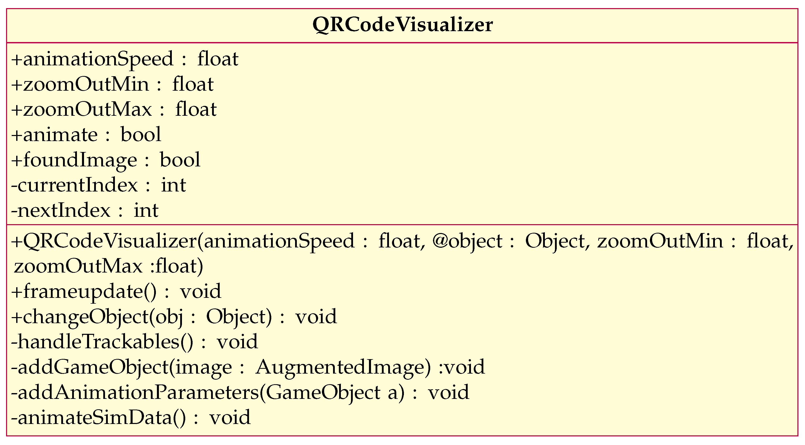
Among other things, the application OpenLBar allows one to visualize simulations above a QR code. As already mentioned, our application is based on Unity and the open-source extension Google ARCore. For this particular case, it was decided to use the functionality trigger image, which allows one to overlay objects and models over a given image. To this end, we implemented a QRCodeVisualizer class dedicated to tracking and managing trigger images, which, in our case, is a QR code. The corresponding class is shown in Figure 5. In essence, the QRCodeVisualizer checks if a trigger image is visible in every frame, and, if yes, if we have already instantiated a SimulationData on it. To save resources, the QRCodeVisualizer checks conversely whether simulation data has been instantiated on the trigger image and whether they are still visible. If this is the case, the simulation data are deleted as they are no longer needed.

As mentioned above, we need some kind of update function that is called at every frame and checks if the AR session is set up correctly as well as whether we are currently actively tracking with the camera. If this is the case, the handleTrackables() method can be called, where all tracked images are checked for visualizations. Depending on the situation, addGameObject() or removeGameObject() is invoked. Another part of the frame update function must be an update of all existing instantiated simulation data, where the scale and position can be changed. As for placement, the visualizer simply places the 3D object at a certain distance above the QR code, depending on its size, and scales the longest side of the object to the length of one side of the QR code. Since the visualizer is responsible for the scale of our object, it is here where we implement a zoom functionality with which one can use two fingers to enlarge or size down the simulation data and obtain a better view of certain areas of the simulation results. The zoomUpdate() method takes user input and converts it into a linear scaling of the simulation data size, either up- or downsizing it depending on the swipe direction. The setMaterial() method can be used to change the point sizes of the point cloud that is used to visualize the simulation results, or its color scheme, and the changeObject() method can be used to change the displayed 3D simulation data to a different one so that one can view a different simulation. With this, we now have a working AR visualization tool for displaying simulation results.

3.2.2. Geometry Overlay

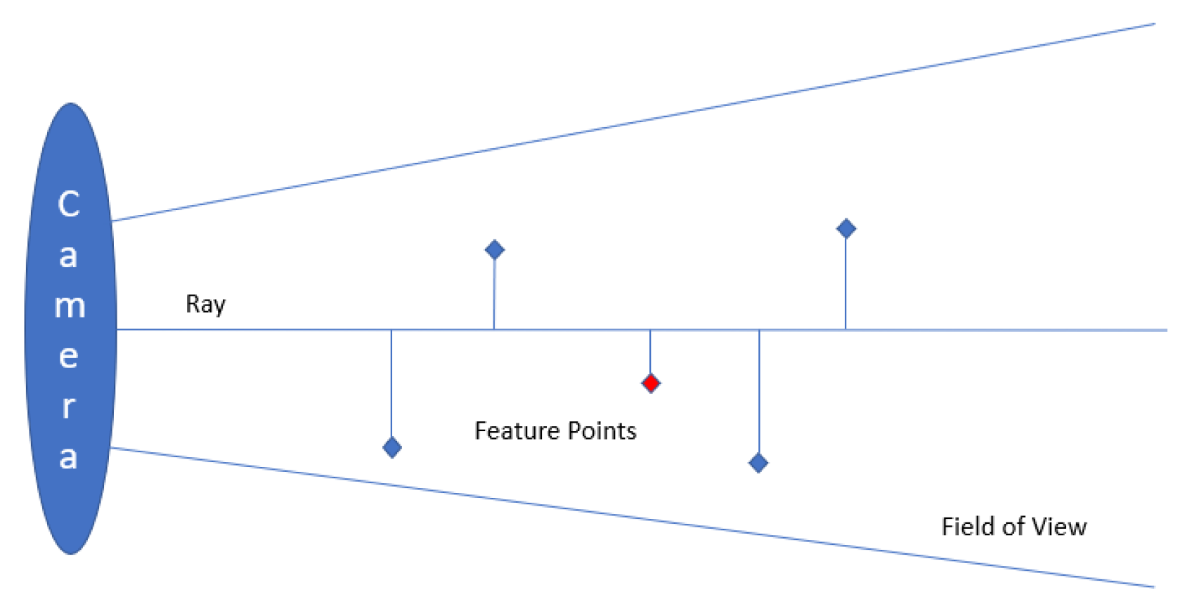
Visualizing simulations on a QR code is a handy method of viewing and interacting with complex processes to obtain a better understanding of the visualized process. However, in certain cases, it is advantageous to overlay the simulation results with an associated geometry to better and more intuitively understand the mentioned process. One of the biggest problems with this type of AR visualization is to figure out where to place the object, how big it is supposed to be, and what rotation needs to be applied. Solid localization is needed for an AR application to be useful and convincing. For the result to be fully utilized, the visualized 3D data must be very close to the original in both position and scale. To achieve this, the functionality feature tracking was used. As the name suggests, this is a process in which distinguishable points are marked and tracked with the phone’s camera. In this case, it was decided to use the built-in feature detection of Google’s AR-Core Library. With it, OpenLBar is able to create a list of notable points in any room and track their positions even when the camera is moving. The next step is to determine the position and scale of our virtual object and fit it to the real object. We realize this by selecting two known points on the object and using the distance between them to scale the virtual object to the appropriate size. However, since we rely on feature detection to track points with the camera, we need to use points that are salient enough for AR-Core to detect. To make the selection process more consistent and user-friendly, we decided to use the edges of our object. The contrast on the edges of the real object allows reliable feature detection there. Thus, it is intuitively clear which points are to be used for scaling. For this edge selection, we implemented a user interface that allows the user to drag a slider over the correct location on the screen. When released, the system automatically finds the nearest feature point.

This is achieved by casting a ray from the selected point on the screen and a ray along the view of the camera, as shown in Figure 6. The distance of each feature point to the thrown ray is then given by

$$d=\frac{\left|\right|(\overrightarrow{p}-\overrightarrow{O})·\overrightarrow{dir}\left|\right|}{\left|\right|\overrightarrow{dir}\left|\right|},$$

(2)

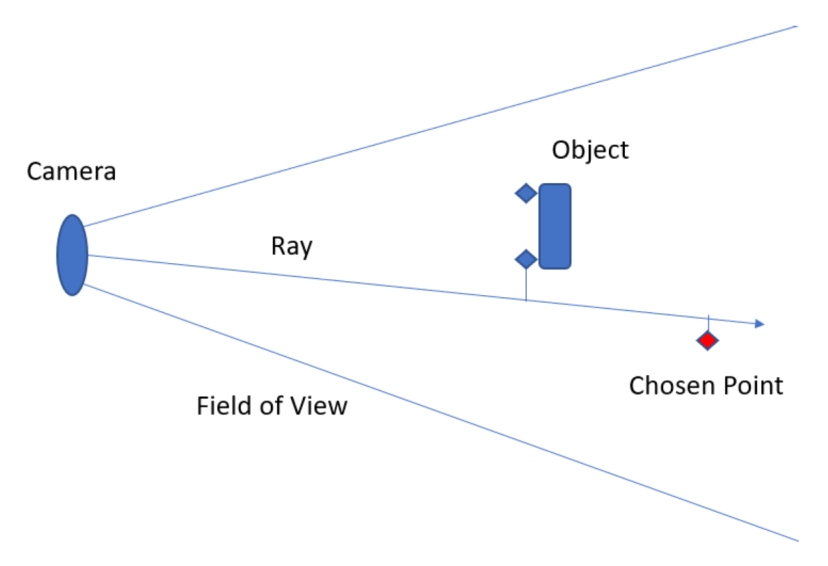
with d representing the distance to the ray, $\overrightarrow{p}$ the location of the relevant feature point, $\overrightarrow{O}$ the position of the camera, and $\overrightarrow{dir}$ the direction of the ray which can be derived from the chosen screen point and the camera rotation. The feature point with the smallest distance to our ray is then selected. However, this method of point selection has one major drawback. Sometimes, this algorithm selects a point that is not at the same depth as the object because a point in the background is closer to the ray, as shown in Figure 7. This leads to significant errors in scaling and rotation. 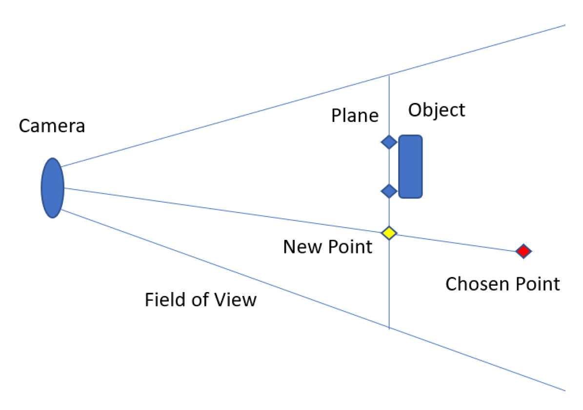Therefore, this error must be taken into account, as shown in Figure 8.

To achieve this, we can consider the object as a plane perpendicular to the camera’s line of sight and draw a line from the selected point to this plane. The intersection of these two is given by

$$\overrightarrow{P_a}=(\overrightarrow{P_2}-\overrightarrow{O})·\frac{\overrightarrow{P_1}·\overrightarrow{n}}{(\overrightarrow{P_2}-\overrightarrow{O})·\overrightarrow{n}}$$

(3)

where $\overrightarrow{P_a}$ is the depth-adjusted feature point, $\overrightarrow{P_2}$ is the feature point to be adjusted, $\overrightarrow{P_1}$ is the closest feature point to the camera, $\overrightarrow{O}$ is the camera position, and $\overrightarrow{n}$ is the normal of the plane and the camera view direction.

The intersection point can now be used as our depth-corrected point to place and scale the virtual object. This results in a much smaller error. We always use the point closest to the camera. The reason for taking this approach is that it is unlikely that the user will have many significant contrasts between himself and the object being viewed. This makes it much more likely that it is the point that is placed on the object. The placement and scaling itself can be performed by calculating the scale factor, which is given by

$$scaleFactor=\frac{modelLength}{realLength},$$

(4)

and we can position it in the middle of the two selected feature points. For objects with a wide base, we are still left with a significant depth error because placement is at the front end of the object; however, since we know how wide the base of the object is, we can move the z-axis back by half the length to compensate for this.

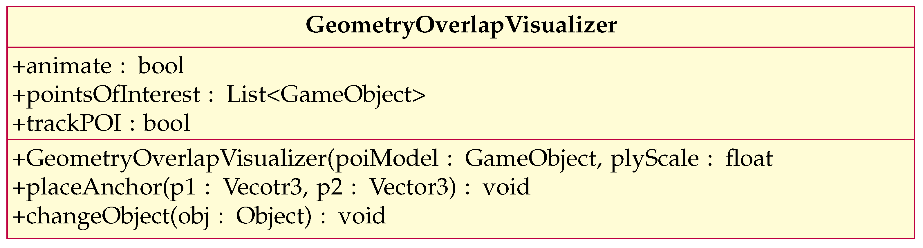
The GeometryOverlapVisualizer implements this functionality using points in worlds’ space as anchors, which are set with the placeAnchor() method. Figure 9 shows all functions that are relevant in order to use the GeometryOverlapVisualizer.

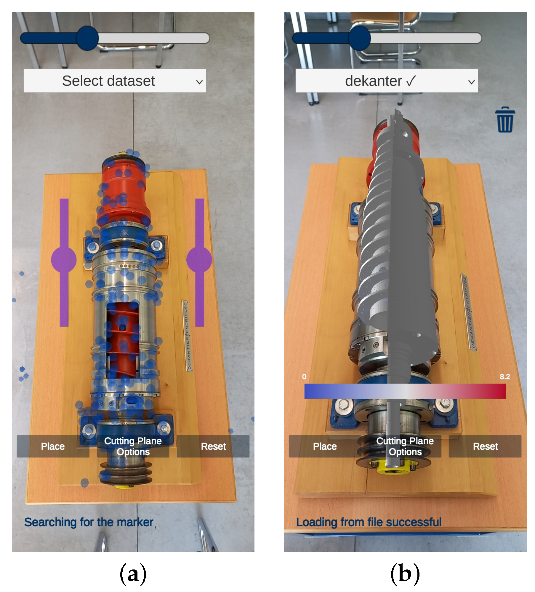
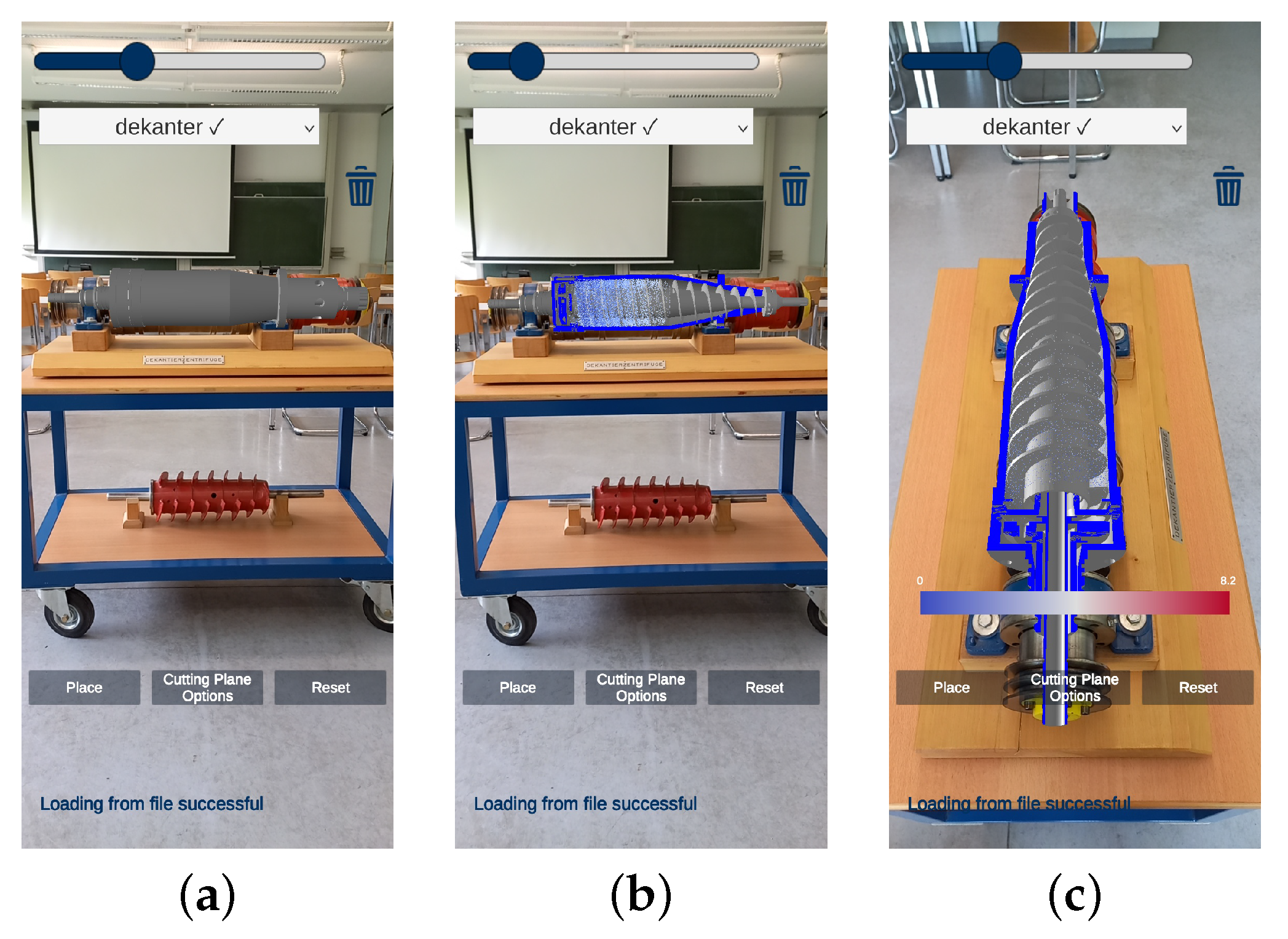
Figure 10a,b show the results using a real decanter and the CAD counterpart.

3.2.3. Animation

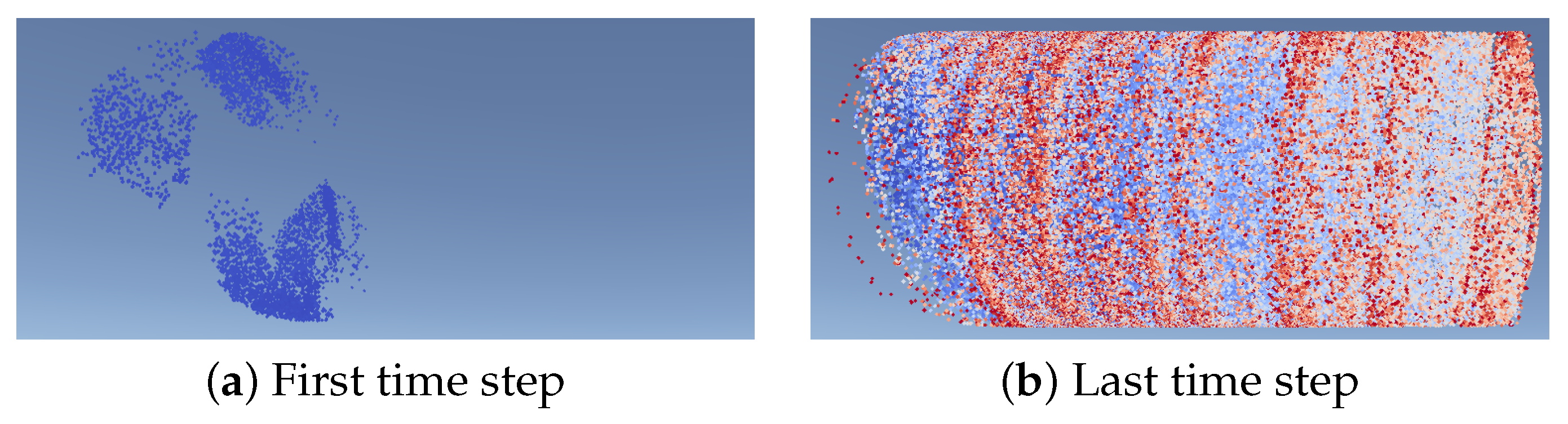
The simulation software OpenLB, which is mainly used for the creation of the simulations, outputs the simulation results as a collection of files of the type Visualization Toolkit (vtk). Each of these files represents a time step of the simulation in question and contains all data in regards to the calculated fields. Using programs such as Paraview, these data can then be converted into different 3D data types, such as the binary GL transmission file format (GLB) or the polygon file format (PLY). On the one hand, the GLB file format could be used. Due to the possibility to save rotations and translations with the 3D file, this is a widely used file format in the AR/VR scene. However, it is not suitable for our purposes because the particle motion of simulations can be very complex. This makes it very costly to store our simulations in a GLB file. For this reason, we decided to convert the data of each time step into a PLY 3D model. In this file format, the 3D data are built up from polygons. They are stored in a list with vertices, triangles, and edges. In this way, we obtain the state of each time step as a 3D file, which can then be shown one after another, creating an effect similar to a stop-motion animation. Figure 11 shows this with the example of a simulation of particles from a decanter. The first time step is shown in Figure 11a and the last is shown in Figure 11b.

In order to achieve the aforementioned effect, a child object named simulation data, with all of the .ply meshes attached as children, is added to our main object. We can then circle through the meshes, activating the next and deactivating the current mesh in order to achieve a fluid animation. Since the method of animation is specific to the case, and we want the library OpenVisFlow to be as expandable as possible, the implementation for the animation falls into the case-specific visualizers, in this case, the GeometryOverlapVisualizer and the QRCodeVisualizer. In this way, it is possible to take advantage of different file formats and animation methods using different visualizers.

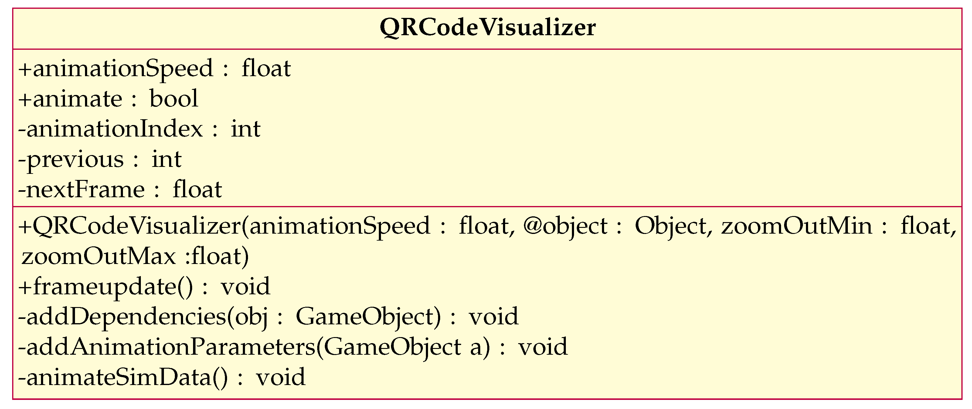
As seen in Figure 12, the animation is controlled using the public float animationspeed and automatically set up for new simulation data, using the addAnimationParameters method, when the changeObject() function is called. The animation is then started with the animateSimData() method, using a background thread, so that it does not become frame-dependent when loading sequences and other calculation-intensive operations are launched.

3.2.4. User Interactions

User interactions are very important to give users a better experience and to make them have more fun exploring. They also help them better understand the results of the simulations. By its very nature, augmented reality provides the ability to view the simulation results from different angles; however, from our perspective, the benefits of AR can be better utilized if additional engaging features are implemented. As already mentioned in Section 3.2.3, we offer users the possibility to control the speed of the simulations themselves. Thus, for example, the user is able to slow down the simulations in order to look at and understand parts of them in more detail. Furthermore, we implemented a zoom function so that the user can scale simulations as desired, making it possible to focus in on specific areas to deepen one’s understanding of the processes at work. To give our application a bit more specificity, we also decided to implement a color legend to make it easier for users to actually use these images to figure out how fast the fluids move at which point in their object. 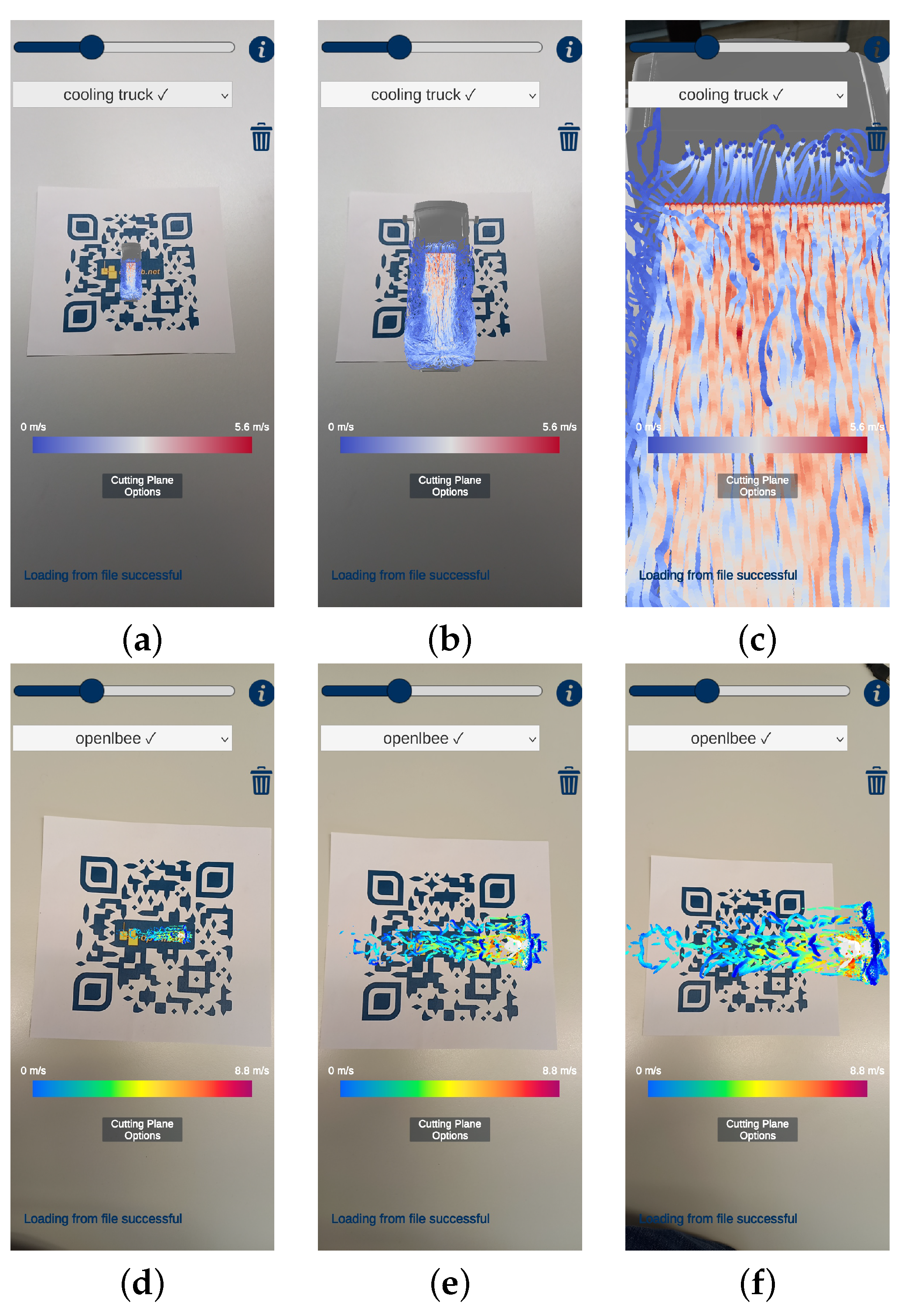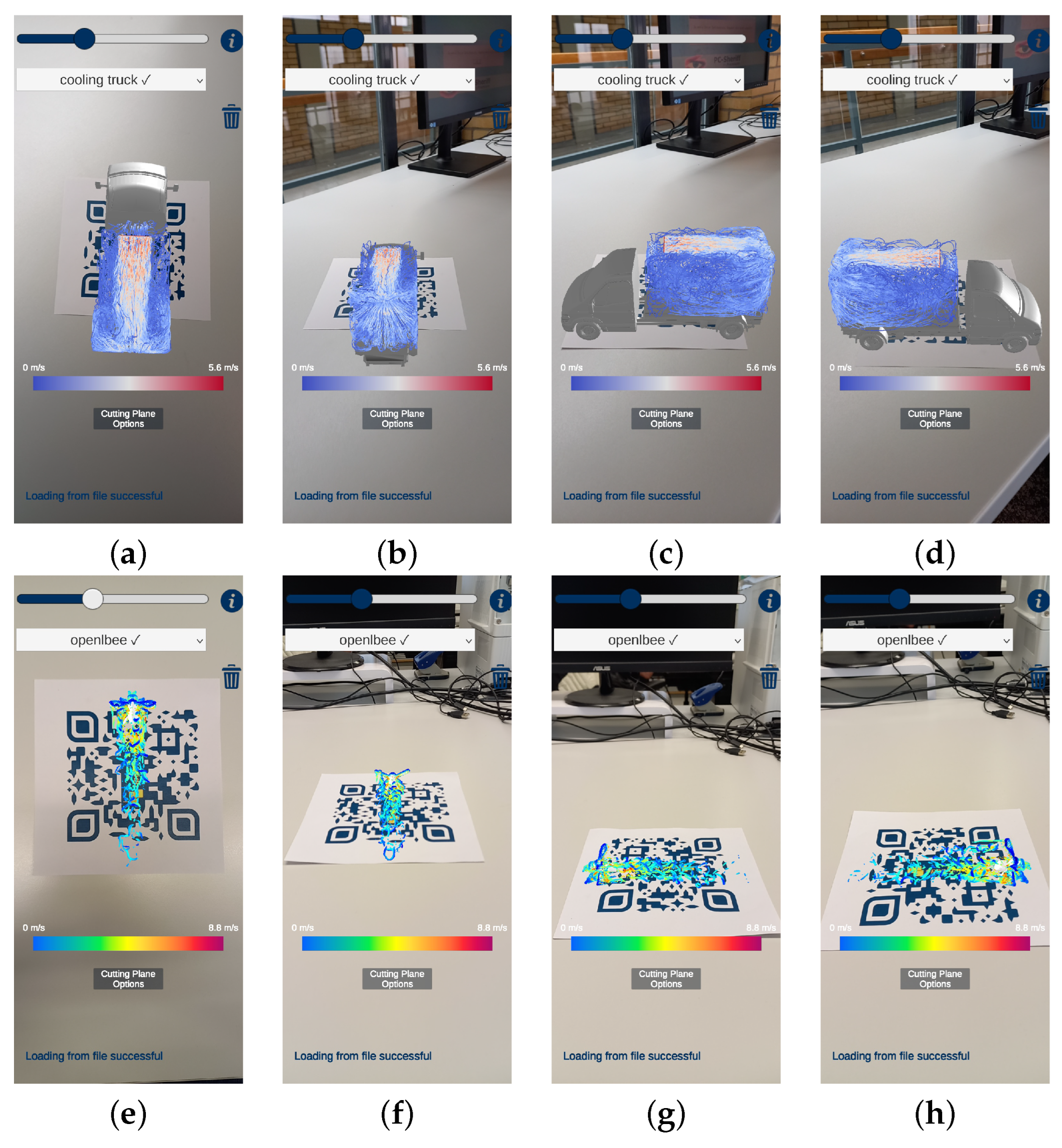Figure 13 shows the zoom function and color legend using the visualization of a cooling truck and a bee.

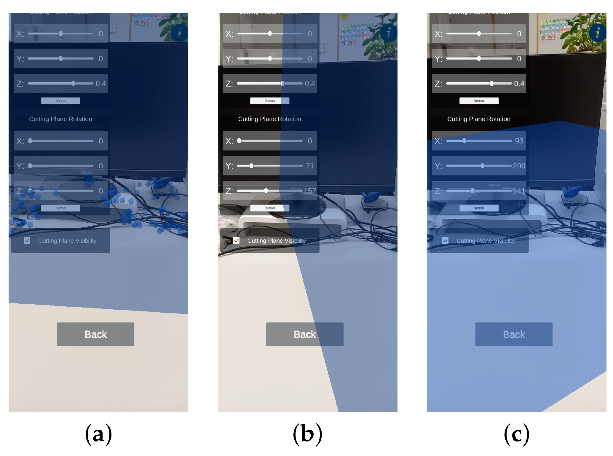
Finally, we wanted to further improve the ability to view virtual data on a real object. To this end, we implemented a way of visualizing only parts of the object. Basically, one can control which parts of the simulation will be shown and which parts will just show the outside wall of the object, giving one the options of seeing cross-section shots and isolating areas for inspection which otherwise would not have been visible behind layers of simulation data. This works by inputting what we call a cutting plane. If a point is on the visible side of it we display it; if it is on the other side we set its alpha to zero, in essence making it invisible. The results of this can be seen in Figure 14. Future versions may include more differentiated methods of defining the visible areas. At the moment, the cross sections are made visible with shaders written by Abdullah Aldandarawy out of the Cross Section Shader add-on from the Unity Asset Store.

3.3. Open-Source Library

Unity is a powerful tool for developing games and AR/VR applications. We see a great potential for teaching, but also for industry to visualize complex processes. This motivated us to start developing a modular open-source library that allows users to quickly, easily, and efficiently develop AR/VR applications for complex processes such as fluid flow. As this paper is also the start of the library, it currently only contains the functionality to create the application OpenLBar presented here. Further functionalities, such as an interface between Unity and the simulation software, such as openLB, will be added soon. In the following sections, the already existing classes and methods of the library are explained. Furthermore, we show how the application OpenLBar can be easily reproduced with its help.

3.3.1. Library Overview

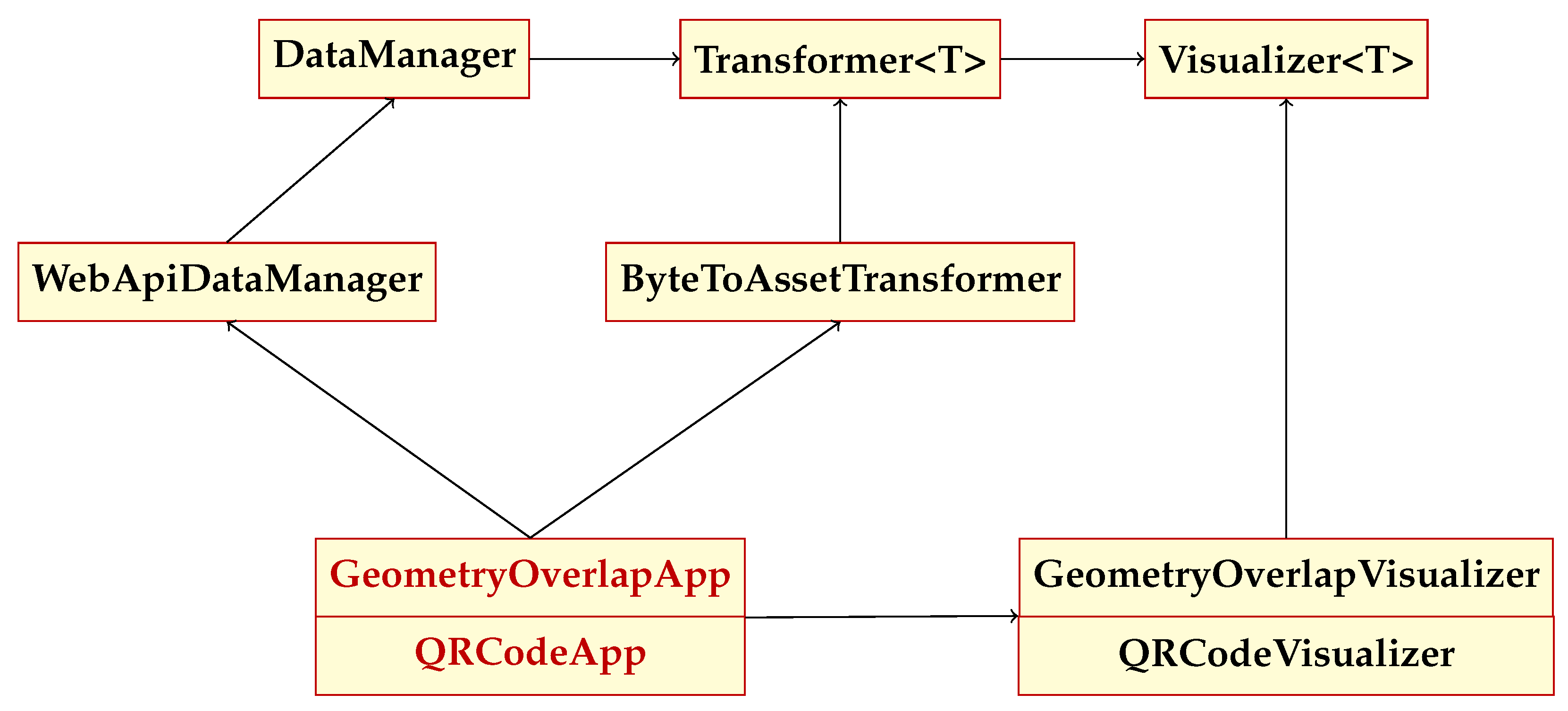
As previously stated, the main goal of this library is to simplify the development process of visualization tools. The library is structured around a main workflow, as can be seen in Figure 15. This consists of three different parts: the DataManager, the Transformer, and the Visualizer. In OpenVisFlow, the DataManager, as its name implies, implements the acquisition and management of incoming data. It is supposed to act as a bridge between our data source and our application to obtain the right data at the right time. The goal is to keep the main workflow as simple and expandable as possible, so the classes DataManager, Transformer, and Visualizer were implemented as abstract, requiring only a few key features and leaving everything except the essentials to a case-by-case implementation of an inherited class. As cases can also vary in the data types required, the implementation of templates was unavoidable; both the Transformer and the Visualizer are dependent on a certain input type of data, which is why both of them are templated to their respective input data type T. In our example we only implemented a single data manager, the WebAPIDataManager, for both cases. The WebAPIDataManager allows the sending of web requests and the subsequent saving and/or loading data as binary files. Next in line is the Transformer, which takes the provided data and transforms them into a form needed by the visualization side. In the example, we implemented a ByteToAssetTransformer, which takes in a byte array and generates a Unity GameObject from it, which can then be used by the Visualizers. As the name suggests, the Visualizers implement the visualization side of the program. In it is the code for animation, placement, and rotation of the Objects in the World. In our example case, we use two different Visualizers, depending on the case. The QRCodeVisualizer enables Visualization above a Triggerimage, in our case, a QRCode. Whenever a Triggerimage is found it will place the GameObject the Transformer supplied right above it. It also implements scaling between a min and max value as well as a public variable for animation speed. For the other case, we implemeted the GeometryOverlapVisualizer, which allows one to overlay an Object in the real World with a virtual twin, by supplying two of the edge points of the object. As of now, the library will only work with Unity as we use Unity GameObjects and AR-Core to realize the AR-visualization. We hope to expand this to Android Studio and other development tools in the future.

As seen in Figure 15, to make OpenVisFlow work, a program needs a class pulling all ties together. This case file needs to hold references to DataManager, Transformer, and Visualizer, and is responsible for controlling all the different aspects of our app through a UI. It also needs to implement some sort of frame update function and call the frameUpdate method of the Visualizer and the DataManager to properly function. The following section will contain more details about the aforementioned classes.

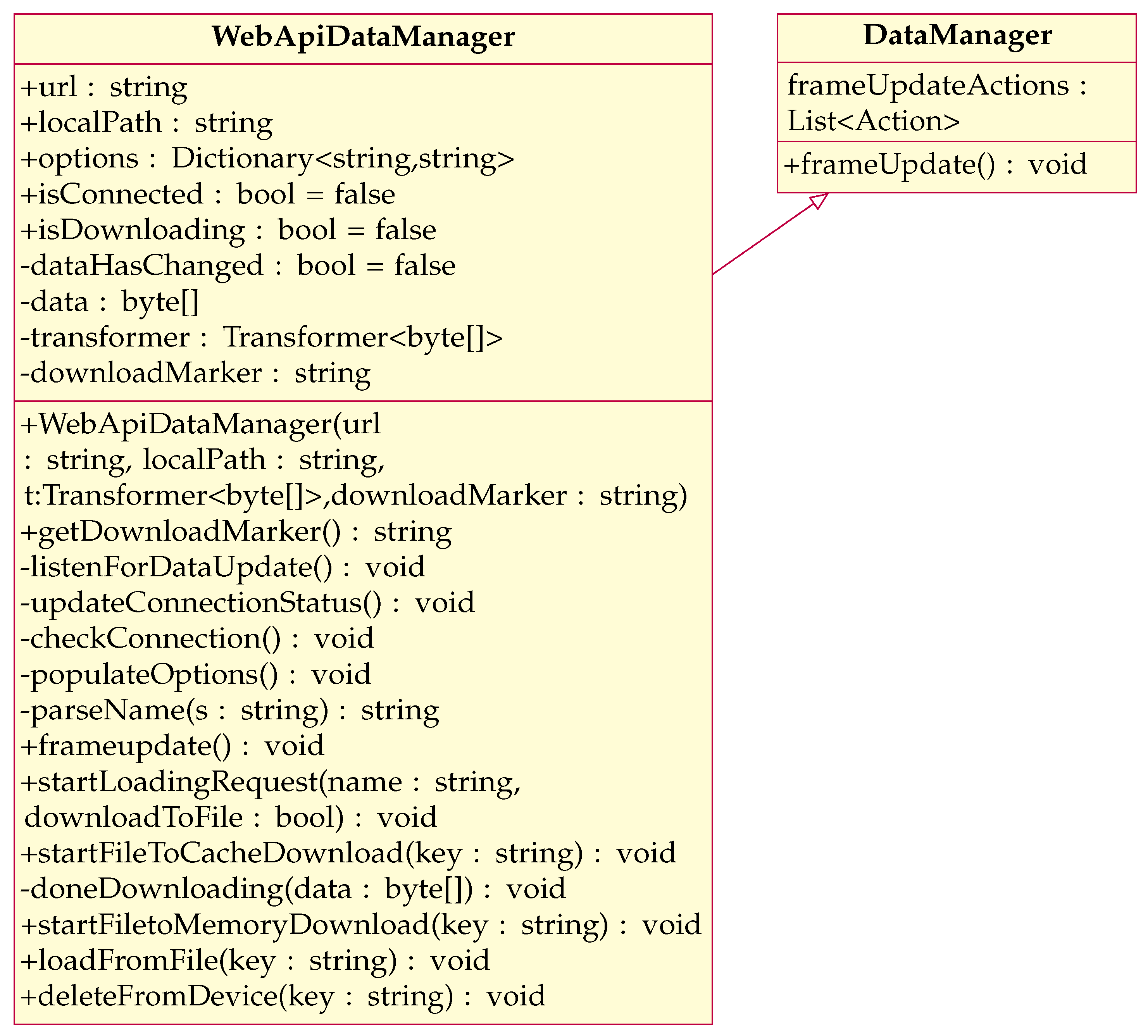
3.3.2. DataManager

As stated above, the DataManager’s main objective is the acquisition and/or management of simulation data. Since these data can be obtained in a variety of different ways and file formats, the DataManagers give the users an easy gateway into the library. Figure 16 shows the WebApiDataManager with all of its functions and how it implements the standard DataManager.

The WebApiManager is supposed to acquire a list of available simulation data from our web server, which it can then download and manage on the local drive of the device. To achieve this, the WebApiManager has two main parts, the first being the populateOptions() function. In it, we check the REST-API and catalog all the available options and compare them to the found data on our device. These options can then be accessed and displayed in whatever way the developer sees fit. Secondly, it gives the developer the option to use these options to initiate a download or local load routine and the following transforming and displaying of said data.

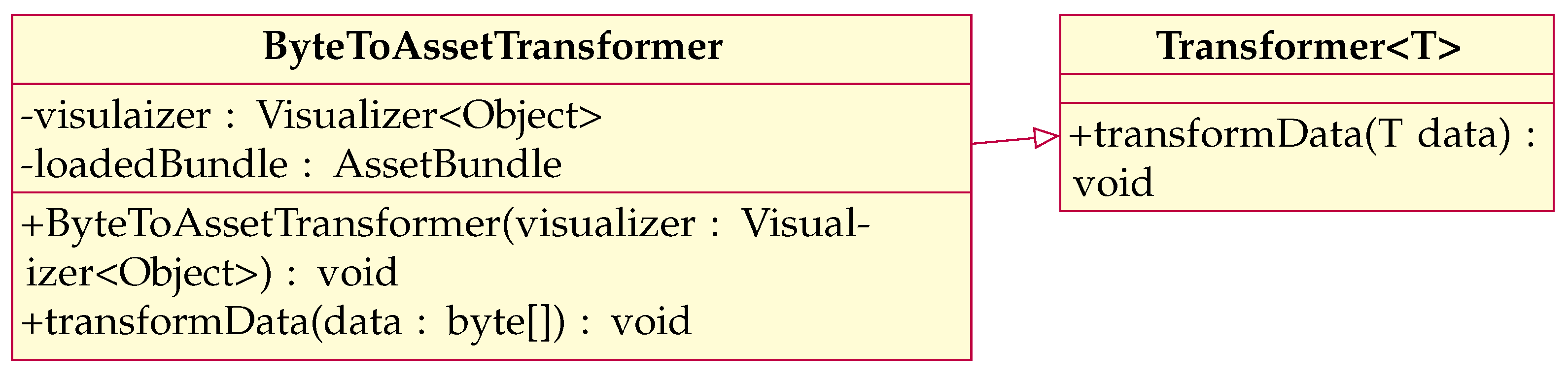
3.3.3. Transformer

Next, we take a look at the Transformer class. It is intended as a bridge between the Visualizer and DataManager, where we can take whatever data are supplied from the DataManager and convert them into whatever form the Visualizer needs. We decided to make an extra Transformer class in order to make it easier to write and add in one’s own Transformers and to keep a cleaner structure for a better overview. In the case below, we read a byte array from an REST website API, and need to convert it into a Unity object in order to visualize it using AR-Core. To this end, the Transformer was implemented as an abstract class templated to the data type it needs to receive from the DataManager. The child then implements both the templated data type as well as the transformData function which can then be called in the DataManager to start the transformation routine. This makes it easier for developers to see which Transformers already exist. At the same time, it is easier to work with a vast variety of different data types. The functions and fields of the transformer, as well as its connection to its parent, can be seen in Figure 17. How the Transformer interacts and relates to the rest of the library can be seen in Figure 15.

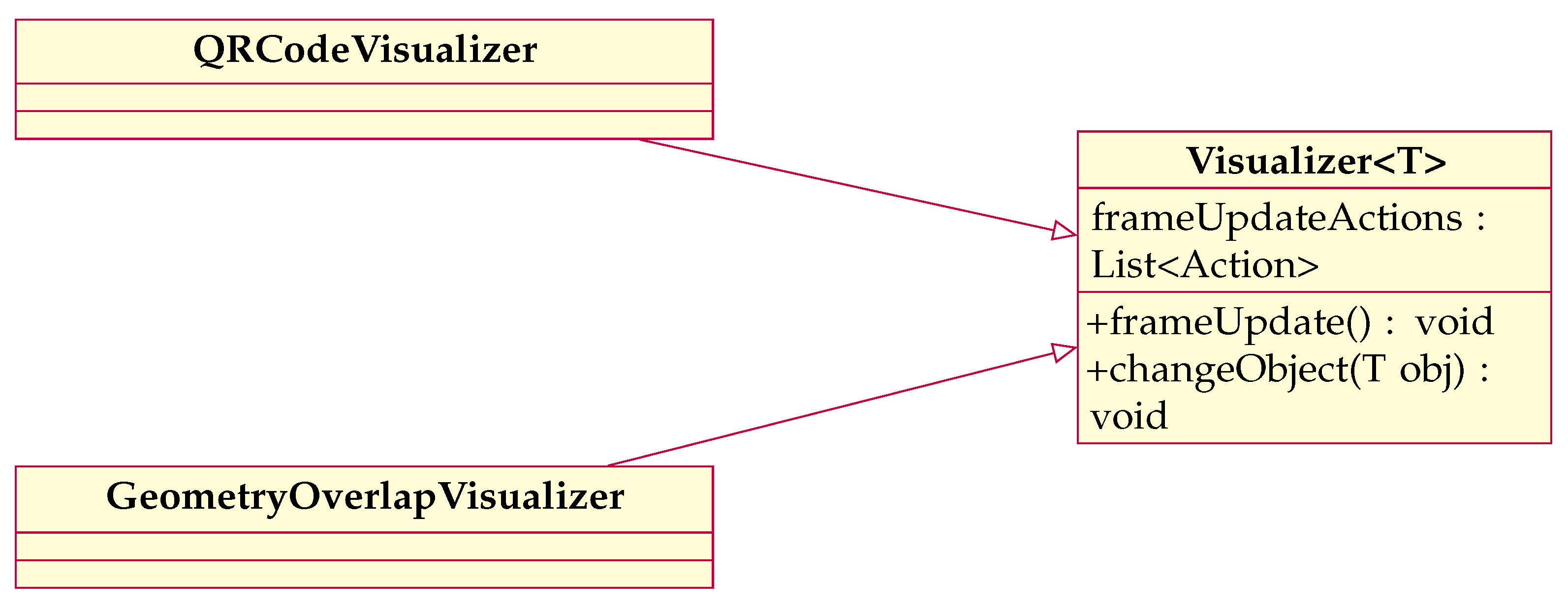
3.3.4. Visualizer

As the name suggests, the Visualizer serves to implement visualization of the data. Since the visualization methods vary widely, the Visualizer needs to be unrestricted by default so the only important decision to make is what data type to use for your visualization and template the child class to it. We only implemented two examples to visualize 3D models in AR using AR-Core, the class diagrams of which can be seen in Figure 18. In this case, we use the Unity object type as our basis for visualization. In the future, we want to implement a variety of different visualization options using VR, AR, and other technologies.

4. Results

In this section, the appearance and fluidity of the resulting animations are discussed. Furthermore, an evaluation with students was performed to determine students’ opinions concerning OpenLBar and AR/VR simulations. Finally, we look at the stability of the QR tracking as well as the accuracy of the manual geometry overlay.

4.1. Quantitative Results

In this section, the OpenLBar application created with OpenVisFlow is tested for its suitability with the help of evaluation forms. The evaluation was conducted with 13 master’s students. Most of the respondents were studying chemical and process engineering. The rest of the respondents studied either mathematics or computer science. The evaluation forms consisted of three sets of questions. The first set is primarily about the handling of the app. Since a practical application must be easy to use, and the installation process and the occurrence of errors or circumstances are mainly queried here. In addition, the first set also asks to what extent the application appeals to the user. In the second set of the survey, sense and usefulness are examined. For this purpose, the respondents were asked to indicate, for example, to what extent they see OpenLBar as a useful supplement to the lectures. In addition, they were asked whether the understanding of engineering problems, especially in the field of fluid dynamics, is simplified by the application. In the third set, exercise tasks were to be examined. For this purpose, the subjects were asked to evaluate the extent to which the exercises provided them with new insights into fluid mechanics. Below, the evaluation of the question sets is discussed.

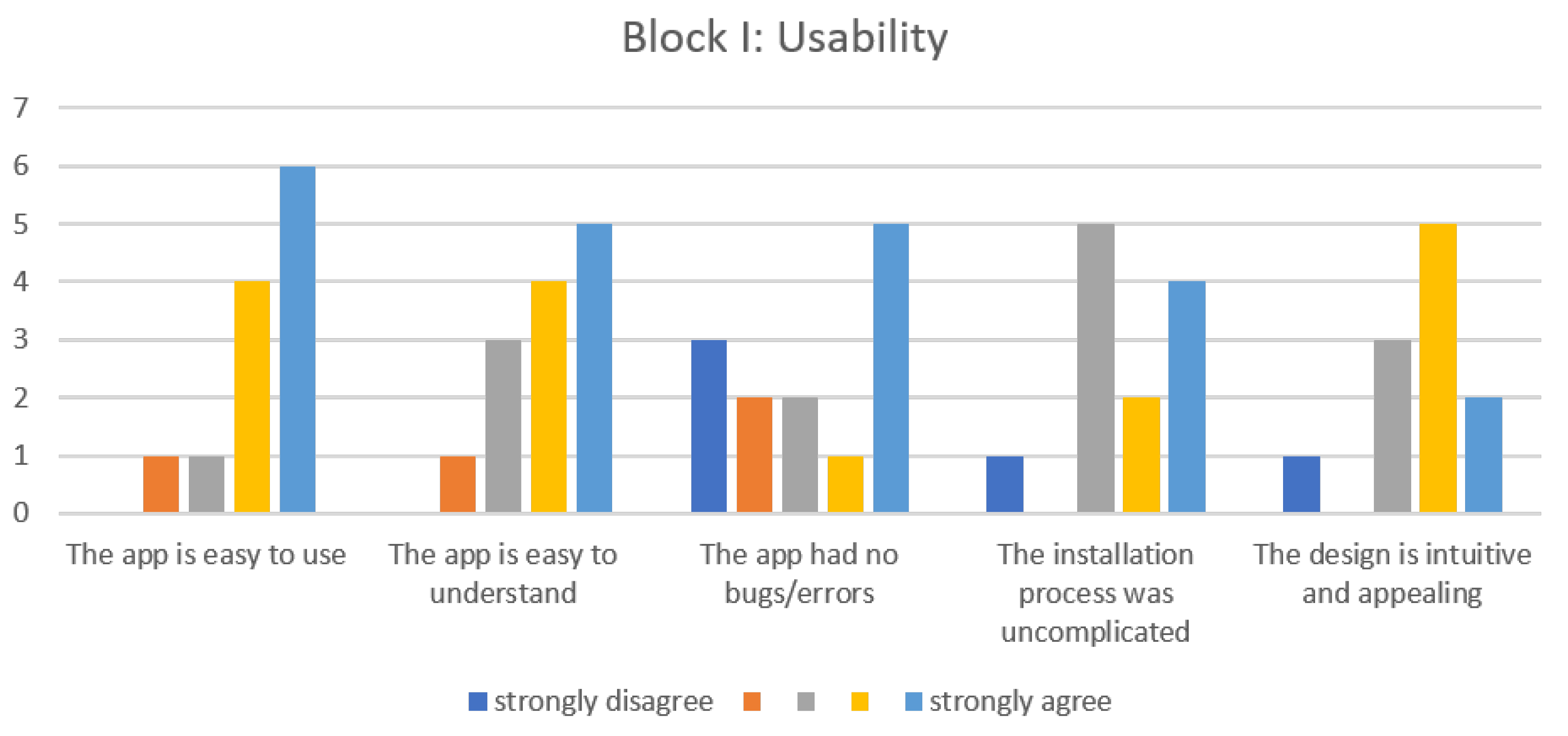
4.1.1. First Set of Questions

Figure 19 shows a diagram of the evaluated questions on usability. As can be seen, the OpenLBar application is an easy-to-use application in the eyes of the students. It is positive to see here that, overall, there is very strong agreement among the respondents. In addition, it is evident from the survey that OpenLBar is easy to understand by the majority, but a certain proportion of respondents encountered comprehension problems. Regarding the question as to whether the application had errors, a similar picture emerges: The majority of the students were of the opinion that no errors occurred; however, a large number of them expressed having encountered problems. The answer as to whether the installation process ran smoothly was answered positively or neutrally by most of the respondents in the positive sense, whereby the neutral attitude made up for the largest share of the results. The last question in the first block, as to whether the design of the application was intuitive and appealing, was answered relatively diffusely. It should be noted that there is a small tendency toward agreement, which is why we assume a positive tendency. Overall, the usability seems to be good, and the application is very easy to understand due to its design and simplicity, while there is still room for improvement in the occurrence of errors.

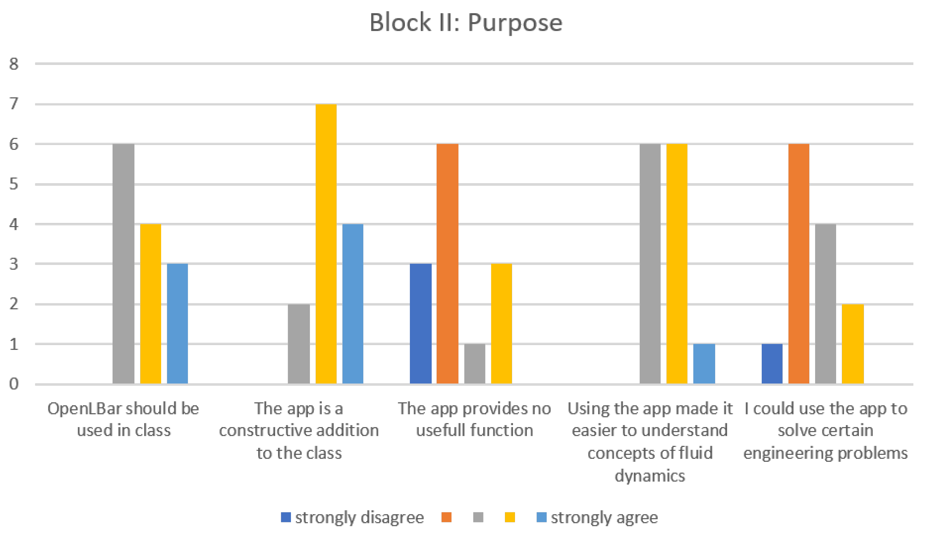
4.1.2. Second Set of Questions

The questions from the second block are used to evaluate the usefulness of the OpenLBar app. The data obtained are shown in Figure 20.

The majority of the students were of the opinion that OpenLBar should be included in the lecture course. It is noticeable that no student was negative toward this statement. At the same time, the neutral stance makes up for the majority of the survey results for the first question. Likewise, a majority of respondents believe that the application is a useful addition to the lecture. Here, too, it is positively noticeable that there are no negative evaluations and there is a strong tendency toward strong agreement. The third question, i.e., as to whether the application does not provide a useful function, was answered quite diffusely. However, it should be noted that the question was deliberately negated in order to stimulate active thinking. Despite the change in question type, it is positively noticeable that the majority of students think that OpenLBar has useful functions. In addition, responses to the question about simplifying the understanding of fluid-named concepts were diffuse as well. Although there is a tendency to agree here as well, it should be noted that there are also many neutral attitudes. One person even completely agrees with this statement. Finally, the last question evaluates the usefulness for solving engineering problems. Most of the students cannot imagine using OpenLBar to solve certain problems. For solving engineering-specific problems, as shown below, students primarily want customizable controllers and parameters. However, they assign high utility to the functionality of the application. Overall, students rate the application’s usefulness as positive. It is noteworthy that some students would like AR applications to be included in academic courses.

4.1.3. Third Set of Questions

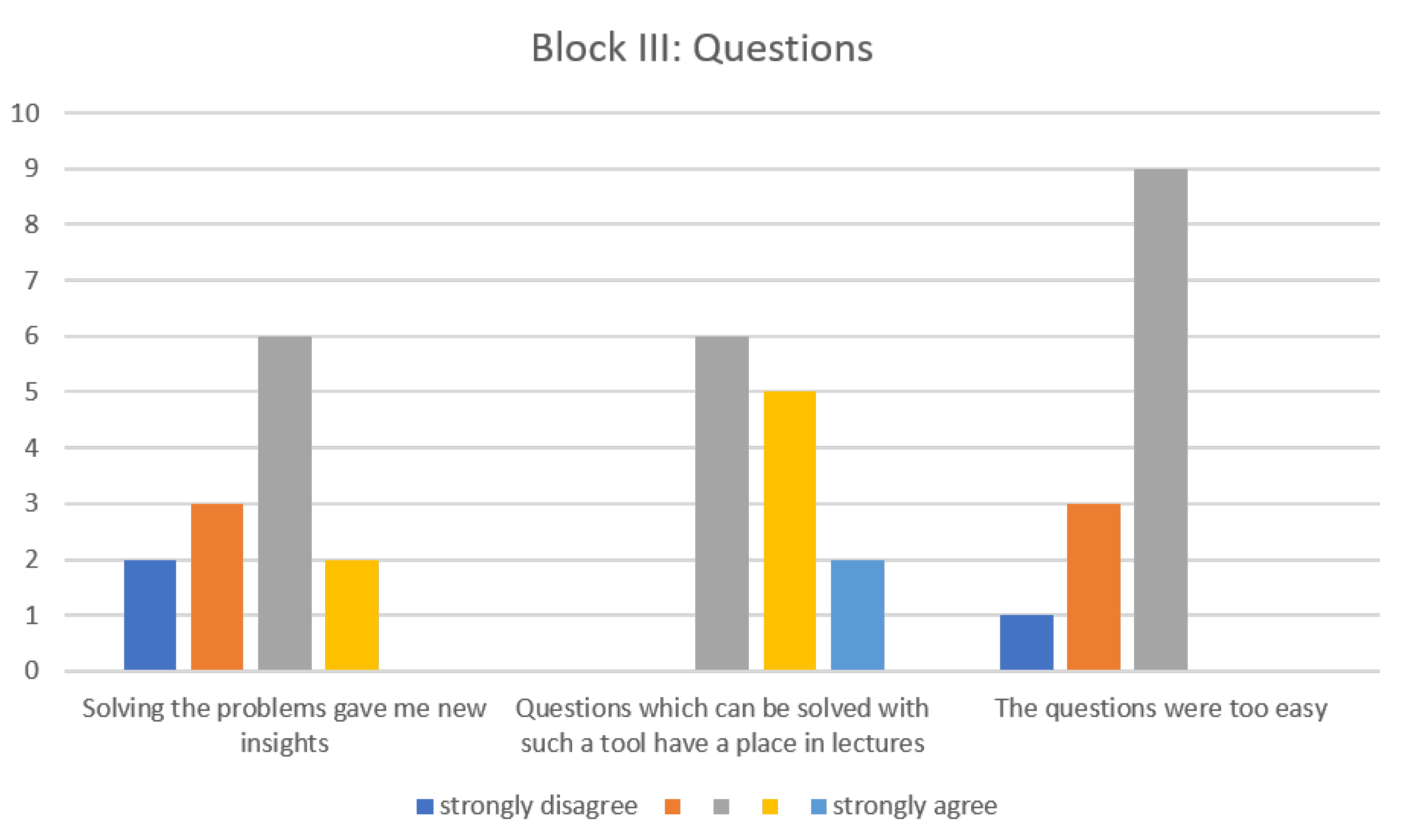
On the evaluation sheet, the students were given tasks to be answered using the application. The first task asked where the air conditioner was located in the cooling truck. The second task asked what conclusion could be drawn about the flow rate of the bee. Afterwards, questions were asked regarding the completion of the tasks. Figure 21 shows the data obtained.

As explained above, the scope of the problems is exactly two examples: on the one hand, the ”cooling truck”, and on the other hand, the ”olbee”. The first question on these tasks aims at gaining knowledge and should clarify whether the students gained new insights into fluid dynamic concepts by working out and solving the case studies. Here, it can be seen that, overall, there is a neutral to negative attitude toward the question. Next, the second question evaluates to what extent general AR applications are a good tool or aid for problem-solving. Here, it is positively noticeable that, in addition to the general tendency to agree, a small group of two people even agree very much. Lastly, the students are of the opinion that the questions were not too easy, with the note that the majority have a neutral attitude. Overall, we can conclude that the application can be useful for solving such tasks.

4.1.4. Free-Response Questions

In the last questionnaire block, students were offered free text blocks to express comments, additions, and other remarks. This was aimed at obtaining more accurate feedback. The question of whether the students encountered difficulties in general was answered by saying that there are still some bugs that need to be fixed. Furthermore, suggestions for improvement were also made. The next question asked was whether AR/VR applications should be integrated into teaching. The overall response was very positive about including modern technologies in teaching. The answers to the question of whether OpenLBar should be used in other lectures were also positive. At last, they were asked the question of what additions to the application would be desirable. Here, it is noticeable that the students would like to adapt the application more according to their needs.

4.2. Qualitative Results

In Figure 22, two example simulations are visualized. Figure 22a–d show a cooling truck, and Figure 22e–h show the simulation of a bee from different angles. It can be seen that the simulations do not have any noticeable flaws at first glance. Furthermore, with the help of the color legend, one can roughly identify the velocities of the flows. In the case of cooling trucks, for example, the velocities are fastest at the exit from the air-conditioning unit mounted on the ceiling of the cargo hold. It can also be seen that the flows slow down over time and approach a constant speed. In the case of the bee, it can be observed that the velocities are zero at the apex of the wings and fastest just beyond. Figure 23 shows the geometry overlay function of a decanter simulation on a real decanter centrifuge. It can be seen that the simulation covers the real object well and all parts of the simulation are still well recognizable.

4.3. Stability

QR code tracking and placing simulations usually do not show any stability problems. However, when viewing the marker at an angle, the position of the object to be placed may not fit exactly. This can be seen, for example, in Figure 22b. If this is ignored, the application is stable in QR mode. On the other hand, the stability of the geometry overlay highly depends on the lighting conditions. The worse the light, the fewer reference points that are detected which enable the geometry overlay. In addition, after placing the simulation, strong camera movements can cause the simulation to shift and no longer cover the real geometry.

5. Discussion

The results presented in Section 4 show that the OpenLBar application is able to visualize simulation data in a sophisticated way for the eye and allows the user to interact with it. This includes, on the one hand, the ability to view the simulations from different angles, given by AR by default. Not to be neglected, however, is the zoom function for looking at parts of the simulation more closely, the cutting plane for removing 3D data that are in the way, and the color legend that allows the user to develop an understanding of the velocities of the moving flows of the simulation. In our opinion, this application is good for the user to obtain insight into complex processes, which are usually not visible. In universities and schools, often only the theory of some topics is taught in class, as visualization is sometimes only feasible with difficulty. Thus, this is an especially useful tool for education to provide students with a representation of theory in the form of simulations. We also see the potential benefit for engineers to see the simulations from a new perspective, as well as a tool to bring the simulations and possible problems closer to the customer. However, AR visualization is not without problems. While it provides one with an easy-to-use intuitive way of viewing simulation data, it is not as well suited to actually work with. Whilst generating graphs, rendering videos, and such functions could all be implemented, they would all come with a significant drawback in usability, since the phone’s touchscreen surface is not the best tool for fine-tuning such selections. Furthermore, AR visualization is dependent on how stable the AR side of the application works. If the tracking does not work properly, the scene will shake and turn in unnatural ways, making proper AR visualization impossible. These problems were solved with the OpenVisFlow library, as it includes a stable AR implementation and provides an interface for ready-made simulations. Thus, the data to be used can be processed externally with powerful tools such as Paraview or Blender.

With this paper, the framework of this vizualization library was implemented and with this, the created application shows a stable and reliable method of visualization.The evaluations in Section 4 show that there is a demand for applications which allow users to interact with CFD simulations in AR; however, they also stated that they want customizable simulations. This cannot be achieved with pre-compiled simulations. Therefore, the main goal of this library is to implement visualization tools, including real time visualization. To achieve this, the next step in the development of this library is the implementation of cluster-oriented tools to visualize simulations just in time.