Predicting Ice Phenomena in a River Using the Artificial Neural Network and Extreme Gradient Boosting

Abstract

Forecasting ice phenomena in river systems is of great importance because these phenomena are a fundamental part of the hydrological regime. Due to the stochasticity of ice phenomena, their prediction is a difficult process, especially when data sets are sparse or incomplete. In this study, two machine learning models—Multilayer Perceptron Neural Network (MLPNN) and Extreme Gradient Boosting (XGBoost)—were developed to predict ice phenomena in the Warta River in Poland in a temperate climate zone. Observational data from eight river gauges during the period 1983–2013 were used. The performance of the model was evaluated using four model fit measures. The results showed that the choice of input variables influenced the accuracy of the developed models. The most important predictors were the nature of phenomena on the day before an observation, as well as water and air temperatures; river flow and water level were less important for predicting the formation of ice phenomena. The modeling results showed that both MLPNN and XGBoost provided promising results for the prediction of ice phenomena. The research results of the present study could also be useful for predicting ice phenomena in other regions.

1. Introduction

Prediction of ice phenomena in rivers is an important element of hydrological regime analysis [1] and the assessment of the risk of ice jam type floods [2]. The changing thermal conditions of river waters during the winter season and the nature of river ice may significantly change the hydro-ecological and socio-economic aspects of the functioning of the river ecosystem.

Due to the stochastic nature of ice phenomena, their prediction is difficult, especially when data sets for rivers are sparse or incomplete. An additional complication is the scale of the event (local and regional scales) and the influence of numerous factors on the process of river freezing, e.g., meteorological (e.g., air temperature, solar radiation, wind velocity) [3,4], hydrological (e.g., flow rate, inflow and outflow conditions) [5,6], the complexity of interactions between hydroclimatic factors [7,8], hydraulic (e.g., trough cross-section geometry, river bathymetry, water table drop) [9] and thermodynamic factors (e.g., water temperature and thermal conductivity) [10,11]. Relations between river freezing and features of the hydrological regime, including flow, water state, and water temperature, are usually complex and non-linear, and are also spatially heterogeneous due to the variability of environmental conditions. In addition to the process that determines the number of occurrences of a given phenomenon, there is also a dichotomous process determining whether it has a chance of occurring in a given period [12]. This task is further complicated by the fact that ice phenomena occur in three phases: freezing of the river (first symptom of ice), permanent ice cover, and the disappearance phase when an ice floe is formed and related phenomena appear, such as ice jams, which often lead to winter floods. However, the full freezing cycle is not always recorded for rivers.

The analysis of time series relating to ice phenomena allows for the determination of the frequency and duration of their occurrence and the tendency of changes over time, and also for an assessment of the ice phases, which provides a good background for the characteristics of the freezing process in many regions. However, it is not sufficient for their prediction and forecasting [13]. Although Shulyakovskii [14] has developed a manual for forecasting the freezing of inland rivers and lakes, there are few studies related to this topic, especially works dealing with the prediction of ice phenomena at various stages of their occurrence. The problem most frequently discussed is the prediction of ice jams on rivers and their consequences in the form of ice jam floods. The theoretical model of river ice jams was developed by Uzuner and Kennedy [15]. Existing forecasts of ice extent are most often based on the location of the 0 °C isotherm [16]. Good results in this regard have also been obtained from observations of river ice ranges carried out with the use of satellites. Remote sensing is useful for the monitoring of ice characteristics, such as different types and thicknesses of ice or ice cover, and for tracking the progress of the breakup of ice jams, which can help predict the location and timing of ice blockages [17,18]. However, the results of field studies and analyses of satellite images do not always provide accurate data for forecasting ice and scenarios of changes in ice dynamics [19].

Prediction models for ice phenomena are usually limited to the empirical or the stochastic due to the difficulties in applying deterministic models. The methods used to predict ice phenomena (e.g., ice jams) include empirical single-variable threshold analyses, logistic regression [2,20], and discriminant function analysis [21]. Many numerical models have been developed to simulate ice formation on rivers [22,23]. According to Wang et al. [24] and Beltaos [25], a better understanding of physical processes has increased the possibility of developing more accurate numerical models of ice jams and ice jam floods in rivers, e.g., the public-domain river-ice RIVICE model [10], the DynaRice model, a two-dimensional coupled hydrodynamic and ice dynamic model [23], and hydraulic models [19]. An interesting ice jam flood forecasting system that considers requirements for the real-time predictions of water, ice, and sediment transport, was developed for the lower Odra River [26]. The prediction of ice phenomena was also carried out using teleconnection indices, as presented by Sutyrina [27] in relation to spring ice phenomena in lakes and reservoirs (including for Lake Baikal).

In the prediction of ice phenomena, machine learning methods are used less frequently, although they have already been utilized widely in forecasting time series of hydrometeorological data [28,29,30]. Artificial neural networks (ANNs) have been used to forecast freezing conditions in rivers [31,32] and predict ice jams [4,33]. For example, Chokmani et al. [34] estimated the thickness of ice using artificial neural networks (ANNs), while Hu et al. [35] predicted the disappearance of ice phenomena using hybrid artificial neural networks. Furthermore, fuzzy logic systems have provided favorable results as regards ice phenomena forecasting and its effects [20,36]. For example, Zhao [3] predicted the breakup date of flood ice using a wavelet neural network (WNN) model. Whereas Yan and Ding [37] proposed a predictive model of ice formation based on a dynamic fuzzy neural network (D-FNN) in combination with a particle swarm optimization (PSO) algorithm. The significant advantages of artificial neural networks over standard statistical classification methods consist in their ability to adapt to data of different formats and configurations [32,34]. Ensemble machine learning methodologies, including resampling methods (bagging, boosting, and dagging), model averaging, and stacking, are used in the solving of problems related to simulation and prediction in hydrology [38,39].

The increase in the amount of hydrological and meteorological data makes it more difficult not only to select the methods for their analysis but also to choose predictive and prognostic models so as to maintain both their legibility and accuracy [40]. For the integrated management of an aquatic ecosystem, it is necessary to determine how the thermal–ice regime of the river will develop and change in the future, considering global climate change and local conditions in particular [41]. The identification of the most important hydrological and thermal variables influencing the course of ice phenomena in a river may result in more accurate forecasts of the freezing process.

The main goal of the present study is to predict ice phenomena in a river with the use of the Multilayer Perceptron Neural Network (MLPNN) and Extreme Gradient Boosting (XGBoost) algorithms, which belong to the group of machine learning methods. MLPNN is one of the most widely used ANN models in the field of hydrology [4,7,8]. According to Zounemat-Kermani et al. [42], the boosting methods (e.g., boosting, AdaBoost, and Extreme Gradient Boosting) are becoming more and more effective for modeling and forecasting water quality, runoff, sediment transport, groundwater, flooding, and drought. One of the advantages of XGBoost compared to neural networks is the ability to assess the importance of predictors in the model, and in this study, by employing the XGBoost model, we can assess the dominant factors controlling the dynamics of ice phenomena in the studied river. The objective of the present research was to show the predictability of the selected models and explain spatial differences in terms of the predictors: air temperature (Ta), water temperature (Tw), water level (H), and river flow (Q), as well as the ice phenomenon of the previous day and of the month of occurrence of the phenomenon. The predictions will be carried out using the example of the Warta River in Poland (Central Europe), which is a river of great economic significance and considerable natural value. The results of the study are important for determining the range of intensification of thermal and hydrological ice phenomena variables and the conditions under which their reduction will occur.

2. Study Area

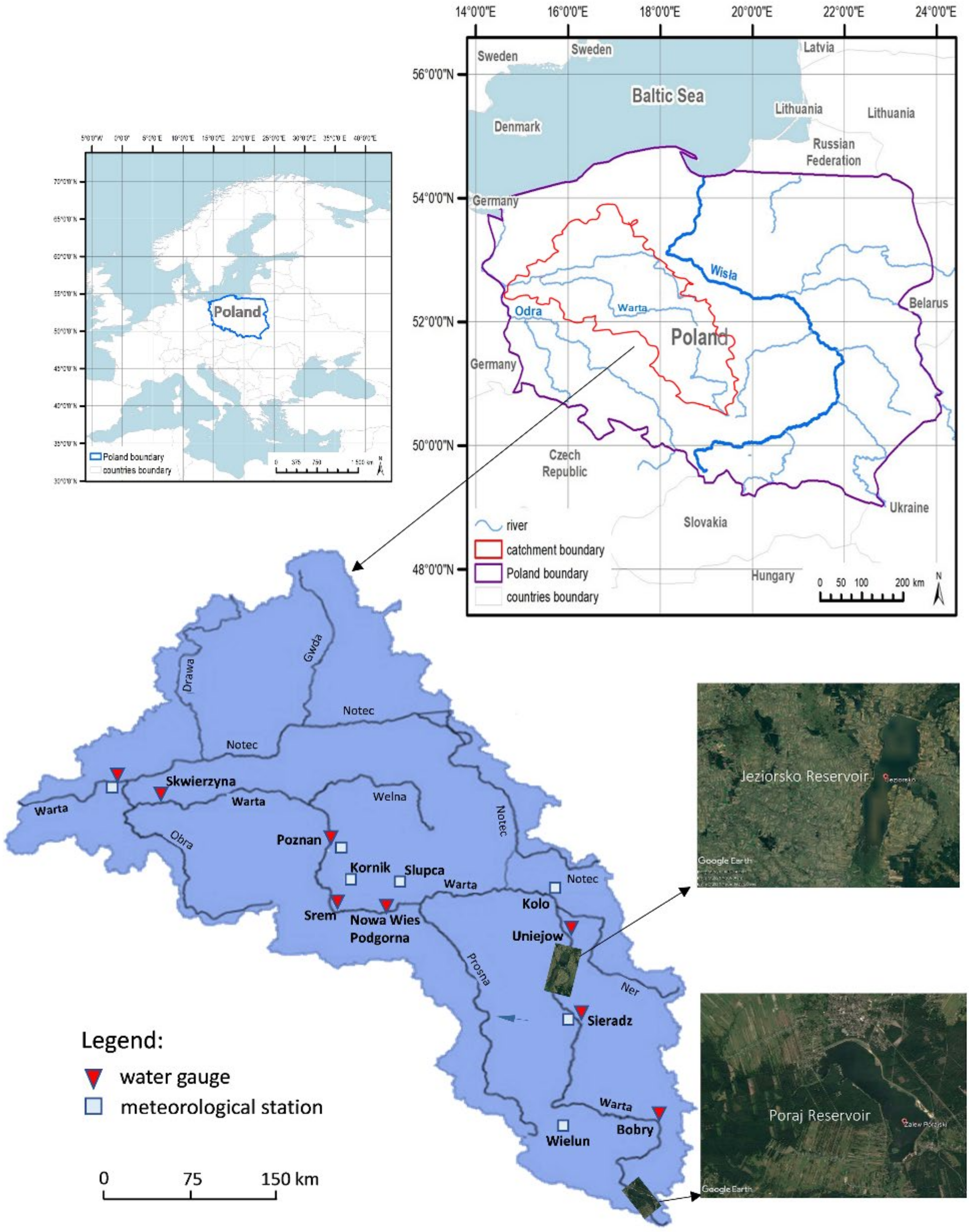
The Warta River is a tributary of the Odra River and the third longest (808 km) river in Poland (Figure 1). Its catchment area (area 54,500 km²) is characterized by a significant diversity of topography and terrain and climatic and hydrological conditions [43]. Within the Warta Water Region there are three main types of relief: old-glacial in the southern part, young-glacial in the northern and central parts, and upland, south of Wielun.

The catchment belongs to nine out of 28 climatic regions designated in Poland by Woś [44]. The average annual air temperature ranges from 7.5 °C in the north to 8.5 °C in the west. In the coldest month—January—the average temperature ranges from −1.2 °C (in the west) to −2.5 °C (in the southeast). Annual rainfall totals in the study area are diverse and range from 520 mm in the Kujawy region (in the northeast) to 675 mm in the south. A regional differentiation of features of the hydrological regime has been observed along the analyzed section of the Warta [45]—from a medium-developed (the upper and lower course of the river) to a highly-developed (along the section from Nowa Wies (Nowa Wieś Podgórna to Poznan) nival regime (Figure 1). The average dates of appearance of ice phenomena on the Warta River, as well as the dates of their disappearance, vary. Research by Graf et al. [46] for the 1991–2010 observation series showed that the earliest ice phenomena occurred in the third decade of December (about 45% of the total number of observations) and the latest in the first decade of January. The disappearance of ice phenomena is usually observed from the end of January to the end of March [47], while about 30% of observations are made in the third decade of February. Most days with ice phenomena on the Warta River are in January (41% of observations), and the most common form of ice is frazil ice (46% of phenomena) and ice cover (30%).

3. Materials and Methods

Predictions of ice phenomena and their numerical descriptions were performed based on daily data on the number of occurrences (the number of days on which the phenomena were observed) and the nature of ice phenomena, and on air temperature (Ta), water temperature (Tw), water levels (H), and river flow (Q) for the years 1983–2013 from the Central Database of Historical Data of the Institute of Meteorology and Water Management—National Research Institute (IMGW-PIB) in Warsaw, Poland (Figure 1). The observation series includes data for the period after 1980, when changes in water temperature in rivers and further consequences, including the lower incidence of ice phenomena, were revealed in response to the sudden climate change associated with changes in CRS (climate regime shift). The regime shift of the late 1980s is a well-documented example of CRS in Poland [48].

Use was made of data from eight water gauges on the Warta River (Bobry, Sieradz, Uniejow, Nowa Wies (Nowa Wieś Podgórna), Srem, Poznan, Skwierzyna, and Gorzow Wielkopolski) and seven meteorological stations (Wielun, Sieradz, Koło, Słupca, Kornik, Poznan, and Gorzow Wielkopolski). Data have been presented in relation to the hydrological year, which in Poland lasts from 1 November until 31 October.

3.1. Classification of Ice Phenomena

The full ice cycle of the river includes forms of ice phenomena observed within the IMGW-PIB water gauge network: frazil ice, border ice, border ice and frazil ice, frazil ice jam, ice cover, ice floes, ice floes and border ice, ice floes and frazil ice, and ice jams. For modeling and predicting ice phenomena, these were grouped into three basic categories: (1) river freeze-up, (2) stable ice cover, and (3) breakup of ice cover—the disappearance of ice (

Table 1. Classification and grouping of ice phenomena.

Class	Ice Phenomena	Ice Phase of the River
	Frazil ice	I phase— Freeze-up
1 class	Border ice
	Border ice and frazil ice Frazil ice jam
2 class	Ice cover	II phase—Ice cover
	Ice floe	III phase— Breakup and ice deterioration
3 class	Ice floe and border ice
	Ice floe and frazil ice
	Ice jam

). The joining into classes is not random, and indeed follows from the order in which ice phenomena appear on the river depending on the thermal and hydrological conditions of the winter season. Each observed ice phenomenon was assigned to the date of occurrence (month and year).

In each of the mentioned phases, characteristic fluvial processes occur as a result of the appearance of various forms of ice. Strictly defined forms, such as frazil ice jams or ice jams, are ephemeral forms. According to data from the IMGW-PIB, in the analyzed period, the Warta River had only several days with frazil ice jams and ice jams, which accounted for 0.1% of all observed ice phenomena. Frazil ice jam embolism occurred on the Warta River in Skwierzyna (three days with jams) and Poznan (one day with jams). Ice jams on the Warta occurred in Srem (three days with jams) and Uniejow (two days with jams).

It should be emphasized that ice jams are not a common event in the Warta River. They are among the characteristic features of the river’s morphology, which makes the reaches of the river susceptible to the formation of frazil ice [46]. In addition, climatic change serves to significantly decrease the intensity of ice jams by increasing the temperature in the vicinity of supercooled water and thereby prohibiting the formation of ice jams. Furthermore, the Warta River is strongly impacted by anthropogenic activity. Regarding the features of its morphology, the Warta River consists of various bed slopes, from mild to steep, which follow each other in a way that affects the pattern of ice formation. Surface ice is observed mainly over the milder sloped beds. Less surface ice is observed over the steeper slopes, while more suspended frazil particles are present. These ice particles may accumulate under the cover of the following flat sections, forming hanging dams at the inlet of the low-sloped sector. There is no specific data for the Warta River regarding hanging dams that would allow us to distinguish between the ice cover itself and frazil depositions with a greater degree of certainty.

3.2. Data Preparation

Predictions of ice phenomena were performed based on daily data on the number of occurrences (number of days with the phenomena) and the nature of ice phenomena and on air temperature (Ta), water temperature (Tw), water levels (H), and river flow (Q), as well as ice phenomena of the previous day (the day before occurrences of ice phenomena from classes 1, 2, or 3, or from class “none”) and the month of individual phenomena (six months of the hydrological winter half-year XI-IV). The choice of input variables was not accidental. The hydroclimatic factors and thermal conditions are important predictors for the process of ice phenomena formation.

To improve the predictability of the tested models and accelerate the process of simulation convergence (in particular as regards artificial neural networks (ANNs)), before inputting the data into Multilayer Perceptron Neural Network (MLPNN) the variables were normalized by converting their values into standardized values (so-called Z-scores) [29]:

$$z_i=\frac{x_i-\underset{\_}{x}}{s{d}_x}$$

(1)

where $x_i$ is the i-th value of x, $\underset{\_}{x}$ is the mean of x, and $s{d}_x$ is the standard deviation of x. The resulting variable z has a mean of zero and a standard deviation of one while retaining all the properties of the original variable. The following variables were transformed: Ta, Tw, H, Q, the day of the month (mon.), and the year (Y).

Additionally, ice phenomena of the previous day, encoded in four columns with the one-hot method (zero for the absence of a given phenomenon, and one when it occurred), and the month of individual phenomena, also encoded with the one-hot method, were introduced into the models. Encoding ice phenomena using the one-hot method with the addition of labels allows the assignment of your own characteristics to specific phenomena, showing the similarities between phenomena or the features that make them different. The ice phenomena data used are treated as categorical variables (also called nominal variables), that is, they represent the types of data that can be broken down into groups. In the tested example, three classes were distinguished (Table 1). However, the categories cannot be ordered from highest to lowest. In the classification methods these variables—as target variables (the ones we want to predict)—are usually converted to numerical form using one-hot coding.

3.3. Descriptive Statistics of the Frequency of Ice Phenomena

The research methodology included several stages. The development of predictive models for ice phenomena on the river was preceded by a statistical description of ice phenomena and their changes in the studied period.

The statistical description of ice phenomena included an analysis of the frequency of ice phenomena in the set of analyzed data, which was determined separately for each measuring station and assuming the classification of ice phenomena into three classes, as presented in Table 1. The next stage concerned the analysis of ice phenomena as sequential phenomena. For this purpose, cross-tables were made comparing ice phenomena from the current day with phenomena from the previous day. In the last step, the relationships between the classes of ice phenomena and air temperature, as well as water temperature, water level, and river flow, were analyzed. For this purpose, box and violin plots were made for the distribution of these parameters for each class of ice phenomenon. The violin plot is a combination of a box plot and a density plot, thus showing more details of data distribution, especially the kernel density distribution [49]. As a result, the problem of overlapping the traditional density plot, which is difficult to identify, is eliminated. Wider sections of the graph signify the higher probability of occurrence of certain values, while narrower sections denote lesser probability. According to Hintze and Nelson [50], the violin plot is used to visualize quantitative and qualitative data, including those that do not conform to the normal distribution, and to define the data structure. Like box plots, violin plots are used to present a comparison of variable distribution (or sample distribution) across different categories.

3.4. Prediction Models

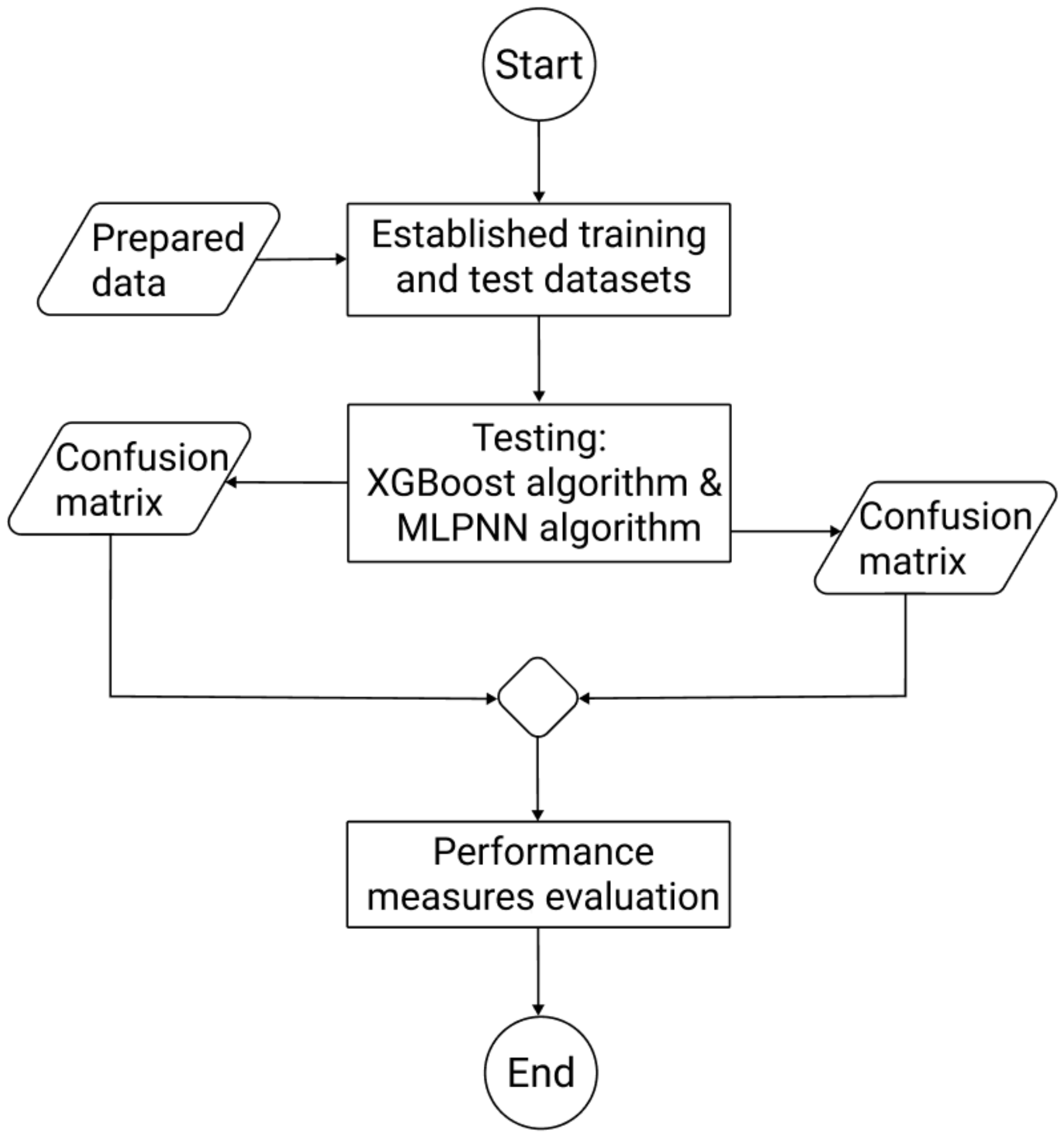
Figure 2 depicts the stages of research activities in brief. The current research was carried out in three stages in total. To begin with, the data that had been cleaned, standardized, and adapted to the needs was referred to as prepared data. The second step was to use the R tools to test model predictions using both XGBoost and MLPNN methods. In the prediction of ice phenomena, the following formula was used (according to the choice of the MLPNN and XGboost algorithms):

ice_0 + ice_1 + ice_2 + ice_3 ~
Ta + Tw + Q + H + D + Y +
day_before0 + day_before1 + day_before2 + day_before3 +
mo1 + mo2 + mo3 + mo4 + mo5 + mo6

(2)

where ice_0 means no ice phenomena, ice_1–3 is the classes of ice phenomena (classes 1–3 adopted on the basis of the classification and grouping of ice phenomena presented in Table 1), Ta is air temperature, Tw is water temperature, Q is river flow, H is water level, D is day of the month, Y is day of the year, day_before0 is day before the day with no ice phenomena (class “none”), day_before1–3 means the day before occurrences of ice phenomena from classes 1, 2, 3 and mo1–6 means months in the winter half-year (November– April, according to the hydrological year).

The training and test sets were created using the stratified sampling algorithm, with the year and month variables functioning as layers. The process of determining datasets is detailed in the description Evaluating the Predictions. The confusion matrices were formed on the basis of the second stage of the activity and were then used as inputs for the third stage, which involved evaluating the performance of the XGBoost and MLPNN methods.

3.4.1. The Multilayer Perceptron Neural Network (MLPNN)

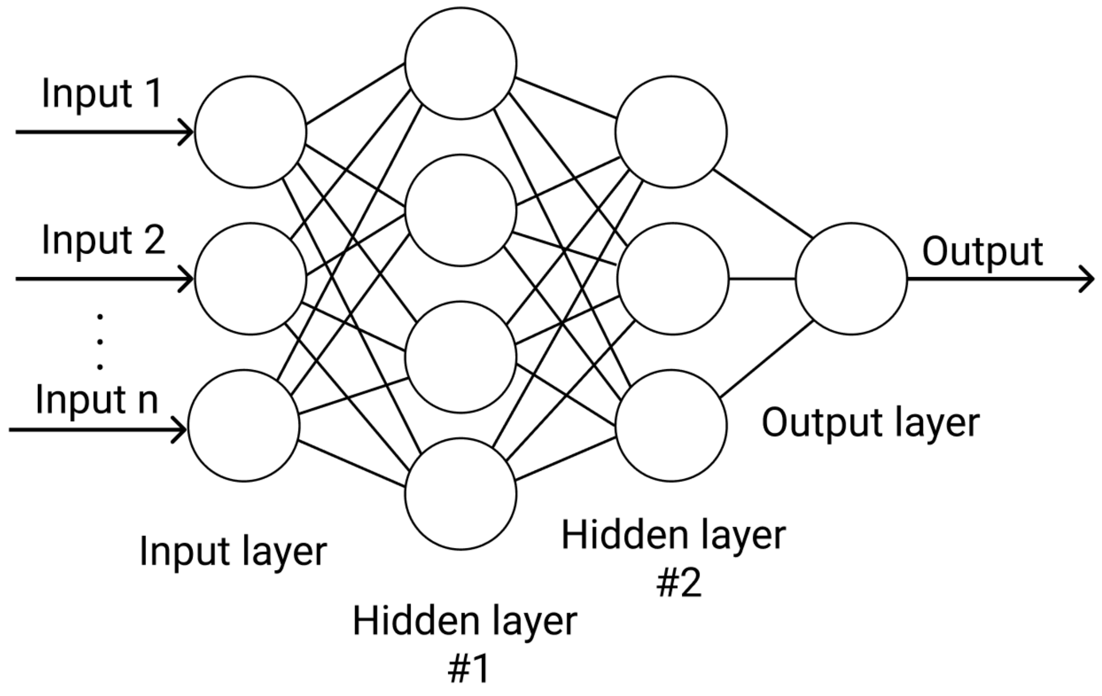
The most commonly used type of neural network method is the multi-layered perception method. In this method, the signal is passed to a one-way loop-free input-to-output network. Neither neuron acts on itself. This architecture is referred to as feed-forward, and consists of multiple inputs, hidden layers, and an output, as shown in Figure 3.

The first model used to predict ice phenomena was the Multilayer Perceptron Neural Network (MLPNN), which included an input layer, one hidden layer, and an output layer, and is one of the most widely used ANN models in the field of hydrology [4,7,8]. The input layer, which comprises the predictors, does not perform any calculations. The hidden layer is made of artificial neurons. A single hidden neuron ‘collects’ activations from each neuron of the input layer and calculates the weighted sum of the input variables. Each hidden layer neuron is connected to each input layer neuron. The hidden layer neurons then perform a non-linear transformation of the weighted sums using an activating function and pass the results to the output layer, which in this application is represented by ice phenomena. A neural network of this type with an output variable Y and containing n neurons in the hidden layer can be expressed as follows [51]:

$$Y=f_2\left[{\displaystyle {\displaystyle \sum }_{j=1}^n}{w}_{jk}\left[f_1\left({\displaystyle {\displaystyle \sum }_{j=1}^n}{x}_i{w}_{ij}+{\delta }_j\right)\right]+{\delta }_0\right]$$

(3)

where $x_i$ is the value of the input variable i, $w_{ij}$ is the weight (synapse) between the input variable i and the hidden neuron j, ${\delta }_j$ is the bias of the hidden neuron j, $f_1$ is the sigmoidal function constituting the activation function for hidden neurons, $w_{jk}$ is the synapse between the hidden neuron j and the output neuron k (here k = 4), $f_2$ is also the activation sigmoid function, and ${\delta }_0$ is the bias of the output layer neuron. The use of the sigmoidal function as an activation function for neurons of the output layer ensured that the predictions would be obtained from the model.

To estimate the weights and biases, the neural net package [52] and implemented elastic back propagation [53] were used. Cross entropy was used as a function of cost. Models with three, four, five, and six neurons in the hidden layer were calculated for each station.

3.4.2. The Extreme Gradient Boosting (XGBoost) Model

The second model tested was the Extreme Gradient Boosting (XGBoost) implemented by Chen et al. [54]—also in the form of the XGBoost library for the R platform. The gradient boosting machine is a team learning technique based on decision trees. A decision tree generates an output variable estimate based on optimized predictor thresholds that divide the data into multiple groups. The gradient boosting algorithm in each subsequent step aims to reduce the prediction error of the previous step. Technically, in each subsequent step the algorithm estimates the parameters of the model whose purpose is to predict the residuals (prediction errors) of the model estimated in the previous step. The objective function (J) in round t (step t) is given by Equation (4) [54]:

$$J^{\left(t\right)}={\displaystyle \sum }_{i=1}^{n}l(y_{i, } {\widehat{y}}_{\begin{array}{c}i\\ \end{array}})+{\displaystyle \sum }_{k=1}^K\mathsf{\Omega }\left(f_k\right)$$

(4)

where: l is the training loss, Ω is regulations, f_k is the function of the K–tree. In this study, $y_i$ is the observed ice phenomena and ${\widehat{y}}_i$ is the obtained final prediction value.

In the present study, decision trees with a maximum depth of five nodes were used. Formally, a tree is any consistent acyclic graph, i.e., a graph that does not contain cycles. The multi-class log loss function was used as the cost function. Predictions of $Y^{\left(t\right)}$ from the model for iteration t are obtained from Equation (5) [39,54]:

$$Y^{\left(t\right)}={\displaystyle {\displaystyle \sum }_{k=1}^t}{f}_k\left(X\right)=Y^{\left(t-1\right)}+f_t\left(X\right)$$

(5)

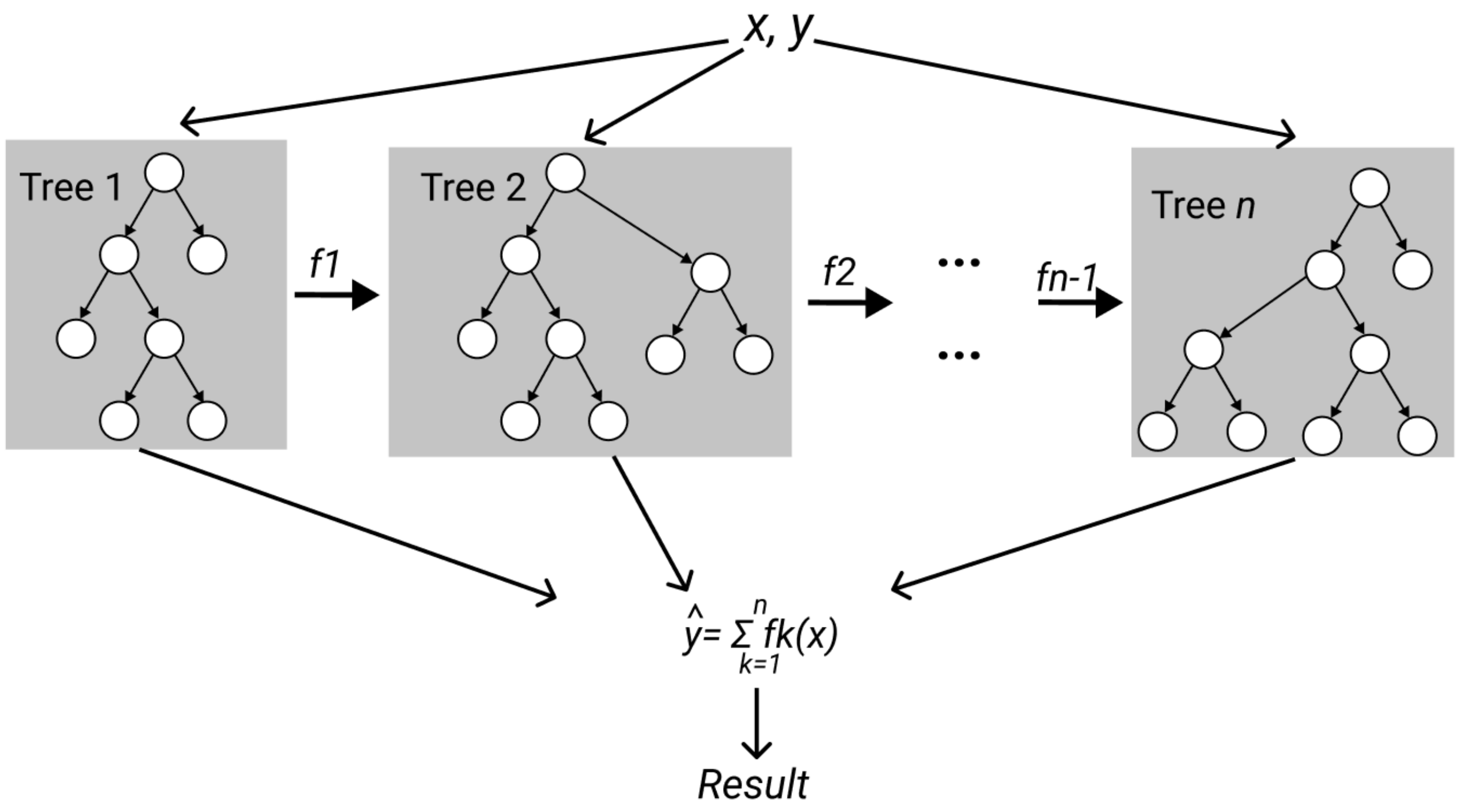
where $X$ is the predictor or set of predictors and $f_k$ is the function that returns the predicted values of the predictors. The second part of the equation shows explicitly that the algorithm prediction in the iteration t is the sum of predictions from the t − 1 iteration and the new predictions from the t iteration. In XGBoost, the function $f_k$ consists of classification and regression trees that enable the modeling of arbitrary nonlinear relations and the prediction of variables of any nature (Figure 4).

One of the advantages of XGBoost compared to neural networks is the ability to assess the importance of predictors in the model. The importance of a predictor for regression and classification trees in the gradient boosting algorithm is defined as the profit that the predictor contributes to the entire model by using it to create successive branches of the tree. In this study, by employing the XGBoost model, we can assess the dominant factors controlling the dynamics of ice phenomena in the studied river.

3.5. Evaluating the Predictions

To assess the predictive power of the tested models, cross-validation and four goodness-of-fit metrics were used. Cross-validation was performed by training the models on the available data (training data) and then calculating predictions and goodness-of-fit metrics for the data on which the algorithms were not trained (test data). The XGBoost model was taught on 70% of the training set, and the prediction model was tested on 30% of the test set. The ANN model was taught on the first 50% of the sample, and the prediction model was tested on the remaining 50%. The test and training sets were created using the stratified sampling algorithm. The year and month variables were used in the form of layers. This was done specifically so that the training and test sets had a comparable number of observations within each year and month included in the analysis. Such divisions are in line with the general practice of evaluating machine learning algorithms [51].

The test and training sets were created using the stratified sampling algorithm, with the year and month variables functioning as layers. As a result, the test and random sets had a comparable number of observations within each year and month.

Four metrics were used as goodness-of-fit metrics, calculated separately for each class of ice phenomena: sensitivity, specificity, precision, and weighted validity [55]. For ease of interpretation of these statistics, consider the following cross tables (

Table 2. Goodness-of-fit metrics.

Prediction	Observation
	Phenomenon	No Phenomenon
Phenomenon	A (TP)	B (FP)
No phenomenon	C (FN)	D (TN)

Explanation: A—TP (True-Positive), the number of true positive predictions, i.e., correctly classified examples from the selected class, B—FP (False-Positive), the number of false-positive predictions, i.e., examples incorrectly assigned to the selected class when in fact they do not belong to it, the so-called false alarm, C—FN (False-Negative), the number of false-negative predictions, i.e., misclassified examples from this class, i.e., a negative decision while the example is positive (the so-called error of miss), D—TN (True-Negative), the number of truly negative predictions, i.e., examples correctly not assigned to the selected class (correct rejection).

), where the letters A–D represent the counts:

The statistics used are defined by the formulas:

Sensitivity = A/(A + C)

(6)

Specificity = D/(D + B)

(7)

Precision = A/(A + B)

(8)

Balanced Accuracy = (Sensitivity + Specificity)/2

(9)

Sensitivity TPR (True-Positive Rate) is a measure of “reach” (coverage, “reaching”) that indicates the percentage of the positive class that has been covered by a positive prediction [56]. Specificity TNR (True-Negative Rate) is a measure of “coverage” that indicates the percentage of the negative class being covered by the negative prediction. Theoretically, Sensitivity (TPR) and Specificity (TNR) are independent measures, however. in practice increasing sensitivity often leads to a decrease in specificity [55]. Precision, referred to as the Positive Predictive Value (PPV), is a measure of precision that indicates how confidently we can trust positive predictions, i.e., the percentage of positive predictions that are positive. The confidence interval for the three distinguished measures is built based on the Clopper–Pearson method for a single proportion. Accuracy is the proportion of correct predictions with a set of test data. It is the ratio of the number of correct predictions to the total number of input samples. In turn, Balanced Accuracy is the arithmetic mean of the recall for each class. The closer the value is to 1, the better the prediction. However, exactly 1 indicates a problem that may be typically labeled as over-fitting. For highly unbalanced classification problems, as in the case of the analyzed data, balanced accuracy is particularly useful, because this statistic depends on both the level of correct prediction of a phenomenon and the level of prediction of the absence of a phenomenon.

Data analyses and operations were performed using the R 4.02 statistical environment [57]. The analyses and the necessary data restructuring, as well as the visualization of the data and the results of the analyses, were performed using the basic functions of the R environment and dedicated libraries for a given type of algorithm. The libraries used are cited in the corresponding analysis.

4. Results

4.1. Probability of Occurrence of Ice Phenomena

The frequency of ice phenomena on the Warta River in the analyzed period has been presented in

Table 3. The frequency of ice phenomena.

Class of Ice Phenomena		Bobry	Sieradz	Uniejow	Nowa Wies	Srem	Poznan	Skwierzyna	Gorzow Wlkp.
1	Nr. of days	518	275	287	417	404	735	449	626
	(%)	10.99	5.8	12.18	10.00	11.73	15.60	10.33	13.29
2	Nr. of days	82	393	130	309	259	69	354	278
	(%)	1.74	8.34	5.52	7.41	7.52	1.46	8.14	5.90
3	Nr. of days	2	45	4	12	4	45	42	15
	(%)	0.04	0.96	0.17	0.29	0.1	0.95	0.97	0.32
No *	Nr. of days	4110	3997	1935	3431	2777	3864	3503	3793
	(%)	87.22	84.86	82.13	82.30	80.63	81.99	80.57	80.50

* No—no ice phenomena.

. At the majority of measuring stations, ice phenomena from class 1 were observed on slightly more than 10% of days, while the frequency of occurrence of phenomena from class 2 varies from about 1.5% to over 8%. Ice phenomena from class 3 (breakup of ice cover—disappearance of freezing) were the least frequently observed. At each measuring station, this class was observed on less than 1% of days.

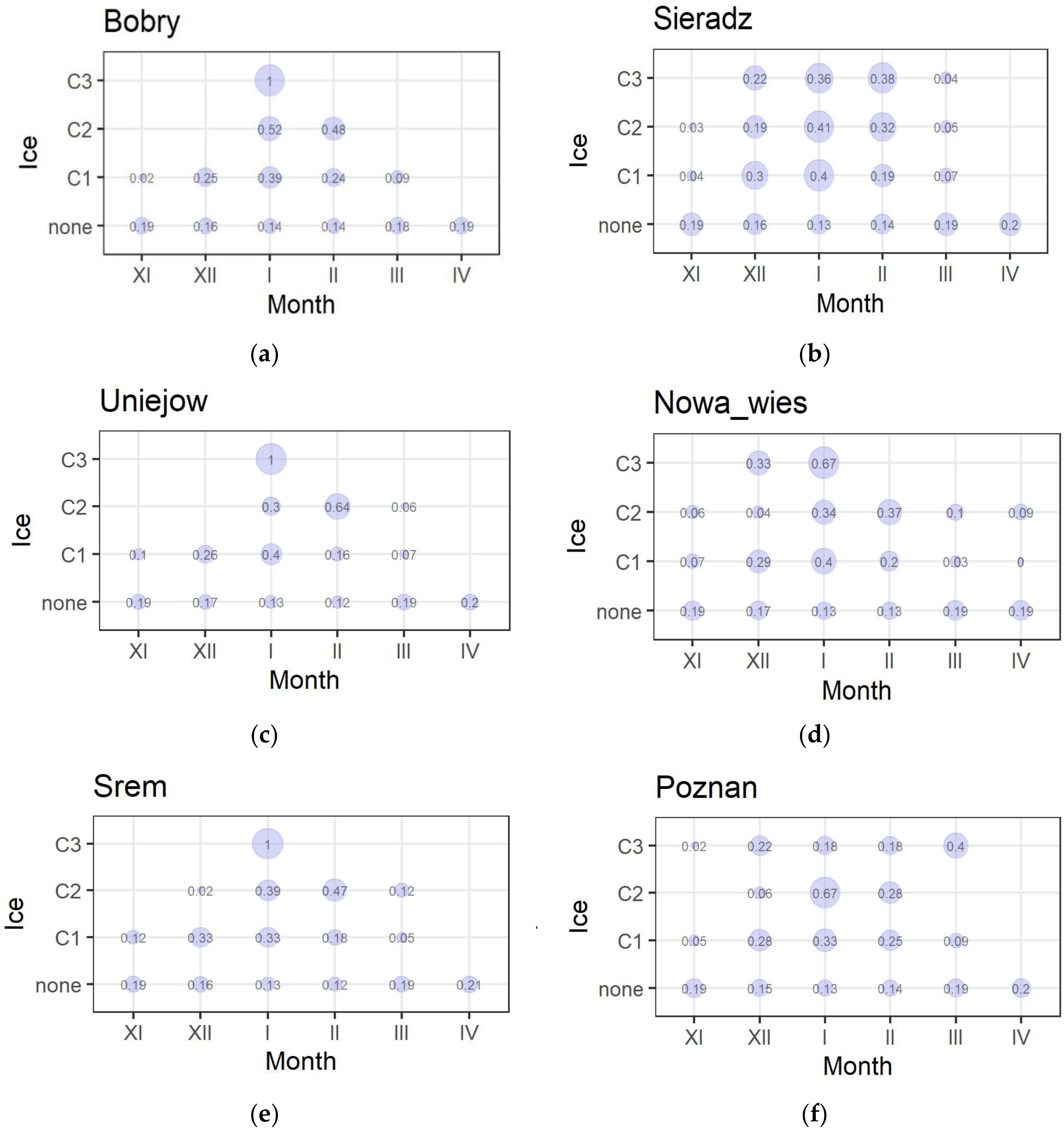
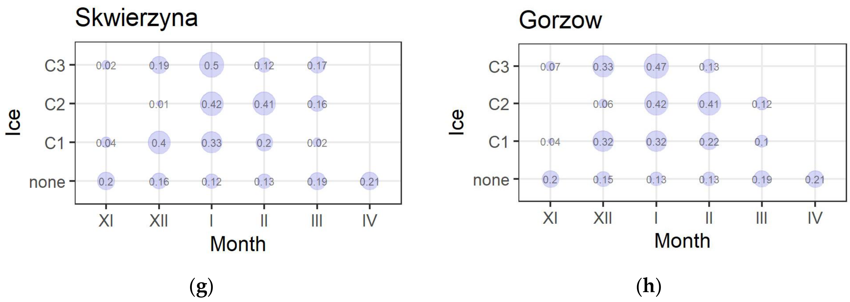
The probability of occurrence of ice phenomena in specific months of the year (in the cold semester of the hydrological year) has been presented in Figure 5. The probability of occurrence of ice phenomena from class 1 is highest in the months of December and January. Class 2 events are most likely to occur in January and February, whereas the greatest probability of the breakup of ice cover and disappearance of freezing (class 3) is associated with the month of January; with February in Sieradz, and with March in Poznan.

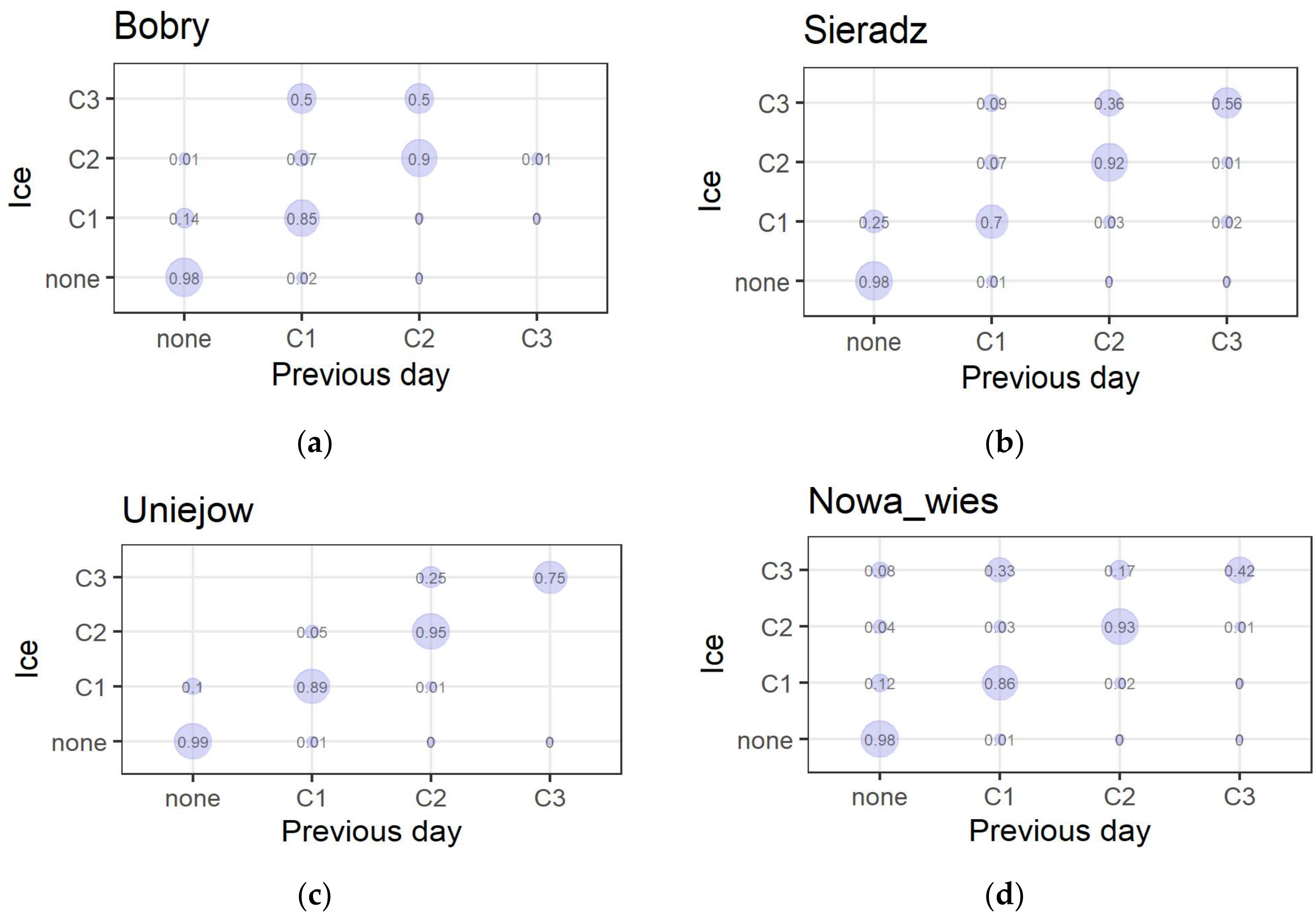
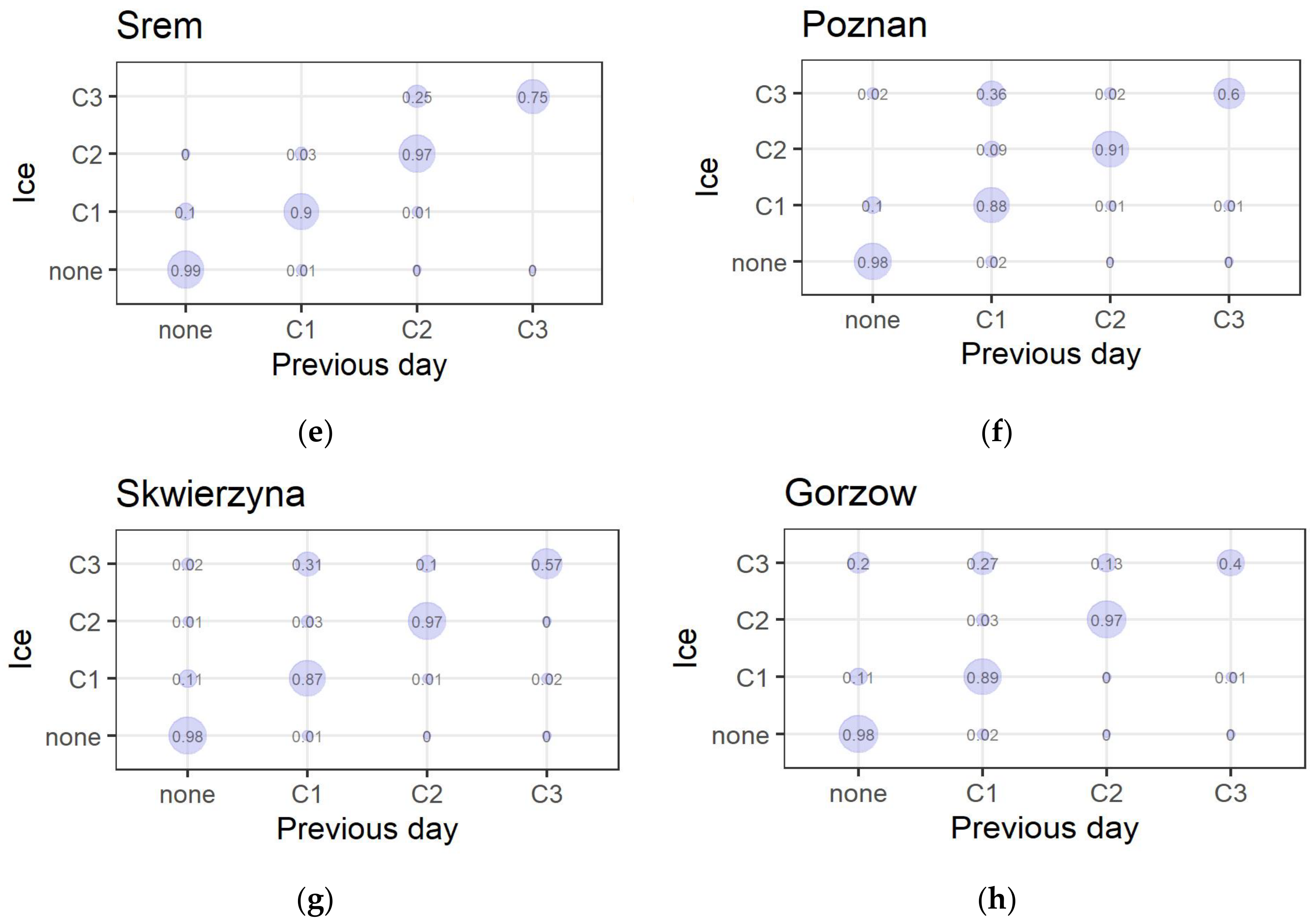
The results of the analysis of ice phenomena as sequential phenomena have been presented in Figure 6. The cross tables compare ice phenomena from the current day with the phenomena of the previous day. It was noted that each class was most often preceded by a phenomenon from its class. Additionally, there was often no ice at all at the river stations the day before the occurrence of ice phenomena from class 1. In a small percentage of days, ice phenomena from class 1 preceded class 2 events. Class 3 occurrences were regularly preceded by phenomena from classes 1 and 2 (Figure 6).

4.2. The Relationship between Ice Phenomena and Hydrological Conditions and Thermal Variables

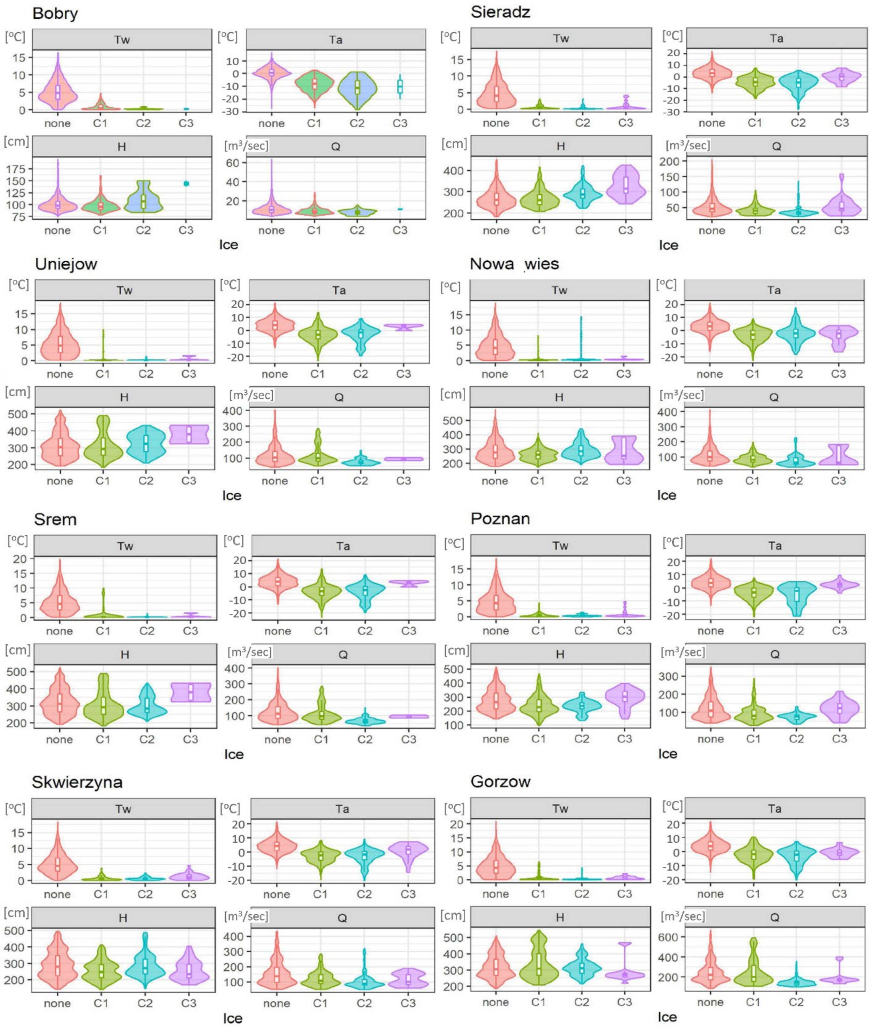
The assessment of the relationship between various classes of ice phenomena and thermal conditions and hydrological factors has been presented in the form of violin plots of the distribution of these parameters for each class of the phenomenon. Figure 7 shows the differentiation of the variables with respect to the water gauges. For each water gauge station on the Warta River, the differentiation of the occurrence of ice phenomena in relation to air (Ta) and water (Tw) temperatures as well as water level (H) and flow (Q) was presented. As drawn, the graphs indicate certain regularities of occurrence of ice phenomena on the river.

The phenomena from the first stage of ice (border ice, frazil ice) are characteristic of the conditions of poor cooling of the water and mild flow, i.e., for the months of November and December. Although frazil ice requires a significant subcooling of the water and an effective dissipation of the heat of solidification, it can form particularly abundantly during strong, cold winds, even if the air temperature drop is insignificant (even at a few degrees below 0 °C). The analysis of the data showed that the ice phenomena from the first phase occur even at a water temperature of the Warta River of 0.2–0.8 °C, and ice cover is maintained at a water temperature of 0.2 °C and at negative air temperatures, which is understandable. In the case of lowland rivers, which also include the Warta River, the ice cover expansion phase, due to low flows and falls, lasts the longest, and its formation is favored by the persistence of negative air temperatures for a long time [46]. The period of ice cover disappearance as a result of an increase in air temperature occurs on the river in stages, as a result of which an ice floe is created that moves downstream (ice procession). The flow of ice floes in the river usually accelerates the cracking of the ice cover caused by the rise in the water level in the spring.

The distribution of ice phenomena concerning water temperature has a distinct character. In this case, the distribution for phenomena classes 1–3 is unimodal and has one high “peak” at very low water temperatures, which indicates the typical regularity of the occurrence of the first ice on the river. Considering the ice cover, the distribution partly takes the form of a slanting distribution with a long tail, which can be seen in the graph for the water gauges of Uniejow, Nowa Wies, and Srem (Figure 7).

As regards the relationship between ice phenomena and air temperature, distribution becomes more diverse depending on the class of the phenomenon and the location of the observation post. For class 1, the distribution is predominantly unimodal. For the majority of measuring stations, distribution is asymmetric and has features of skewed distribution. At the Sieradz and Skwierzyna stations, this distribution shows a tendency to bimodality, which would suggest the presence of two characteristic periods of air temperature and thus favor an increase in the probability of occurrence of ice phenomena from the first phase in these locations. In the case of class 2 (permanent ice cover), distributions at almost all stations are unimodal with a clear skew towards very low air temperatures, which strongly suggests that the probability of ice cover is related to the accumulation of days with negative air temperature. The exception is the Poznan water gauge, for which distribution has features similar to the bimodal distribution (Figure 7). For class 3 (breakdown of the ice cover), the distribution has features typical of unimodal distribution and is focused on an air temperature ranging from 0 °C to a few degrees above zero. This form of relationship is typical of most water gauges on the Warta River. Finally, as regards the water gauges in Nowa Wies and Skwierzyna, the skewness of the distribution increases, and this points to an increase in outliers.

The distribution of ice phenomena from class 1 (formation of ice phenomena) concerning the water level displayed predominantly bimodal features (Figure 7). In the case of the Bobry and Sieradz stations, the distribution shows features of asymmetry and develops as a skewed distribution. In the case of distributions with two or more mods, the widest sections of the violin diagram indicate the greatest probability of observing ice phenomena on the river at a low and medium water level. However, additional periods with a specific water level on the Warta River (states above the average) at which ice phenomena will occur under favorable river thermal conditions are not excluded. The bimodal distribution indicates that the distribution of ice phenomena in this relationship is unstable or very variable. Distribution displays similar features in the case of the relation of the ice cover (class 2) to the state of the water, which is also bimodal at most stations (Figure 7). The distribution shows similar features as regards the relation between the ice cover (class 2) and the state of the water, which, too, is bimodal at the majority of water gauges. The exceptions here are Sieradz and Poznan, for which a unimodal distribution with a specific skewness has been identified. For ice phenomena from class 3, the relationship with the water level shows different types of distributions: unimodal (Poznan and Gorzow Wlkp.) and biomodal (Nowa Wies and Skwierzyna). In the case of Sieradz, the distribution is flat, while in Gorzow Wlkp. it is strongly skewed.

The distribution of the relationship between ice phenomena from class 1 and river flow is bimodal at Nowa Wies, Poznan, and Skwierzyna and unimodal at other stations (Figure 7). In the case of Uniejow, Srem, and Gorzow Wlkp., distribution is also strongly skewed. The greatest probability of occurrence of ice phenomena in the initial period of the Warta River’s freezing is associated with the low flow of the river. In the case of permanent ice cover (class 2), the distribution is unimodal at all water gauges, except for Nowa Wies, where it exhibits features of bimodality. This means that the distribution of ice in this relationship is relatively stable along the entire river. However, as regards ice phenomena from class 3, the distribution at certain stations has unimodal (Uniejow, Srem, and Gorzow Wlkp.) or bimodal (Sieradz, Nowa Wies, and Skwierzyna) features.

4.3. Predicting Ice Phenomena

The results of predictive modeling have been presented for three sections of the Warta River: the upper course (Bobry, Sieradz, and Uniejow water gauges)—

Table 4. Results of predictive modeling of ice phenomena for the Warta River (upper course).

Water Gauge	Model	Class	Training Set				Test Set
			Sensitivity	Specificity	Precision	Balanced Accuracy	Sensitivity	Specificity	Precision	Balanced Accuracy
Bobry	XGBoost	* No	0.986	0.892	0.985	0.939	0.984	0.852	0.978	0.918
		1	0.87	0.987	0.888	0.928	0.83	0.982	0.852	0.906
		2	0.93	0.997	0.87	0.964	0.872	1	0.971	0.936
		3	-	1	-	-	0	1	-	0.5
	NN3	No	0.988	0.907	0.987	0.947	0.982	0.861	0.979	0.922
		1	0.874	0.987	0.892	0.931	0.811	0.983	0.863	0.897
		2	0.978	0.998	0.917	0.988	0.919	0.994	0.723	0.957
		3	1	1	1	1	0	1	0	0.5
	NN4	No	0.988	0.928	0.989	0.958	0.98	0.886	0.984	0.933
		1	0.905	0.988	0.905	0.947	0.844	0.982	0.844	0.913
		2	0.933	0.998	0.913	0.966	0.946	0.995	0.761	0.971
		3	1	1	1	1	0	1	-	0.5
	NN5	No	0.988	0.921	0.988	0.954	0.98	0.876	0.982	0.928
		1	0.909	0.987	0.898	0.948	0.863	0.979	0.833	0.921
		2	1	1	1	1	0.791	0.998	0.872	0.894
		3	0	1	-	0.5	0	1	-	0.5
	NN6	No	0.998	0.934	0.99	0.966	0.982	0.855	0.979	0.918
		1	0.928	0.997	0.972	0.962	0.831	0.981	0.844	0.906
		2	0.927	1	1	0.963	0.829	0.997	0.829	0.913
		3	-	1	-	-	0	1	-	0.5
Sieradz	XGBoost	No	0.992	0.919	0.985	0.955	0.983	0.936	0.989	0.96
		1	0.765	0.987	0.807	0.876	0.869	0.977	0.675	0.923
		2	0.934	0.989	0.895	0.962	0.912	0.995	0.943	0.954
		3	0.2	1	0.8	0.6	0.28	1	0.875	0.64
	NN3	No	0.983	0.965	0.993	0.974	0.973	0.917	0.986	0.945
		1	0.88	0.983	0.767	0.932	0.774	0.974	0.644	0.874
		2	0.961	0.992	0.917	0.977	0.957	0.993	0.922	0.975
		3	0.37	0.997	0.556	0.683	0.444	0.999	0.8	0.722
	NN4	No	0.991	0.928	0.987	0.959	0.98	0.915	0.985	0.948
		1	0.739	0.991	0.836	0.865	0.686	0.982	0.701	0.834
		2	0.99	0.994	0.934	0.992	0.959	0.987	0.869	0.973
		3	0.591	0.997	0.684	0.794	0.522	0.999	0.8	0.76
	NN5	No	0.997	0.929	0.987	0.963	0.984	0.852	0.976	0.918
		1	0.77	0.996	0.919	0.883	0.559	0.986	0.696	0.772
		2	0.976	0.992	0.917	0.984	0.952	0.991	0.904	0.972
		3	0.643	1	1	0.821	0.412	0.997	0.467	0.704
	NN6	No	0.992	0.947	0.991	0.969	0.982	0.888	0.98	0.935
		1	0.871	0.993	0.89	0.932	0.684	0.983	0.715	0.833
		2	0.99	0.992	0.919	0.991	0.954	0.984	0.851	0.969
		3	0.273	0.999	0.75	0.636	0	1	-	0.5
Uniejów	XGBoost	No	0.986	0.922	0.983	0.954	0.993	0.941	0.988	0.967
		1	0.873	0.983	0.879	0.928	0.912	0.99	0.926	0.951
		2	0.938	0.996	0.938	0.967	0.969	0.999	0.984	0.984
		3	0	1		0.5	0	1	-	0.5
	NN3	No	0.994	0.971	0.994	0.983	0.981	0.892	0.976	0.936
		1	0.951	0.992	0.945	0.972	0.818	0.98	0.854	0.899
		2	0.969	0.999	0.984	0.984	0.97	0.995	0.914	0.982
		3	1	1	1	1	0	1	-	0.5
	NN4	No	0.993	0.977	0.995	0.985	0.979	0.927	0.984	0.953
		1	0.974	0.989	0.931	0.982	0.881	0.978	0.838	0.93
		2	0.919	1	1	0.96	0.956	0.996	0.942	0.976
		3	1	1	1	1	0	1	-	0.5
	NN5	No	0.998	0.958	0.991	0.978	0.98	0.835	0.965	0.908
		1	0.954	0.997	0.98	0.976	0.756	0.978	0.816	0.867
		2	0.951	1	1	0.975	0.855	0.999	0.983	0.927
		3	1	1	1	1	1	0.997	0.333	0.998
	NN6	No	0.999	0.986	0.997	0.993	0.99	0.888	0.976	0.939
		1	0.98	0.999	0.993	0.989	0.804	0.989	0.91	0.897
		2	1	1	1	1	0.938	0.993	0.884	0.966
		3	1	1	1	1	0	0.999	0	0.5

* No means no ice phenomena.

; the middle course (Nowa Wies, Srem, and Poznan water gauges)—

Table 5. Results of predictive modeling of ice phenomena for the Warta River (middle course).

Water Gauge	Model	Class	Training Set				Test Set
			Sensitivity	Specificity	Precision	Balanced Accuracy	Sensitivity	Specificity	Precision	Balanced Accuracy
Nowa Wies	XGBoost	* No	0.988	0.904	0.979	0.946	0.984	0.91	0.981	0.947
		1	0.855	0.988	0.896	0.922	0.867	0.983	0.846	0.925
		2	0.948	0.995	0.936	0.972	0.896	0.994	0.926	0.945
		3	0	1	-	0.5	0	1	-	0.5
	NN3	No	0.989	0.917	0.982	0.953	0.98	0.89	0.976	0.935
		1	0.86	0.99	0.899	0.925	0.819	0.985	0.864	0.902
		2	0.956	0.994	0.933	0.975	0.94	0.991	0.887	0.965
		3	0	1		0.5	0	1	-	0.5
	NN4	No	0.984	0.933	0.986	0.958	0.986	0.842	0.966	0.914
		1	0.901	0.985	0.872	0.943	0.805	0.986	0.868	0.896
		2	0.929	0.997	0.96	0.963	0.838	0.994	0.921	0.916
		3	0.4	0.998	0.333	0.699	0.143	1	0.5	0.571
	NN5	No	0.979	0.95	0.989	0.965	0.981	0.91	0.981	0.946
		1	0.93	0.981	0.844	0.955	0.827	0.985	0.861	0.906
		2	0.956	0.997	0.968	0.977	0.906	0.991	0.888	0.949
		3	0.625	1	1	0.812	0.25	0.996	0.111	0.623
	NN6	No	0.987	0.966	0.992	0.976	0.972	0.919	0.983	0.946
		1	0.967	0.989	0.911	0.978	0.898	0.973	0.791	0.936
		2	0.957	0.998	0.975	0.977	0.865	0.994	0.921	0.93
		3	1	1	1	1	0.167	0.998	0.2	0.582
Srem	XGBoost	No	0.99	0.936	0.984	0.963	0.991	0.935	0.985	0.963
		1	0.895	0.99	0.921	0.942	0.903	0.989	0.917	0.946
		2	0.969	0.997	0.962	0.983	0.945	0.999	0.984	0.972
		3	0	1		0.5	0	1	-	0.5
	NN3	No	0.992	0.982	0.996	0.987	0.976	0.927	0.982	0.951
		1	0.967	0.993	0.949	0.98	0.876	0.977	0.829	0.926
		2	0.984	0.998	0.969	0.991	0.955	0.998	0.977	0.977
		3	0.667	1	1	0.833	0	0.999	0	0.499
	NN4	No	0.997	0.962	0.991	0.98	0.99	0.894	0.976	0.942
		1	0.94	0.997	0.981	0.968	0.82	0.99	0.912	0.905
		2	1	1	1	1	0.931	0.996	0.945	0.963
		3	1	1	1	1	0.333	0.998	0.25	0.666
	NN5	No	0.999	0.957	0.99	0.978	0.988	0.905	0.977	0.947
		1	0.929	0.997	0.979	0.963	0.874	0.986	0.896	0.93
		2	0.977	1	1	0.988	0.877	0.998	0.974	0.938
		3	1	1	1	1	0.5	0.998	0.25	0.749
	NN6	No	0.997	0.976	0.994	0.987	0.98	0.912	0.979	0.946
		1	0.95	0.997	0.975	0.974	0.822	0.983	0.869	0.903
		2	0.993	0.999	0.985	0.996	0.992	0.994	0.925	0.993
		3	1	1	1	1	0.333	0.999	0.333	0.666
Poznan	XGBoost	No	0.987	0.922	0.983	0.955	0.984	0.889	0.975	0.937
		1	0.906	0.983	0.906	0.945	0.874	0.98	0.893	0.927
		2	0.935	0.999	0.906	0.967	0.895	0.999	0.919	0.947
		3	0.567	0.998	0.81	0.782	0.267	0.998	0.5	0.632
	NN3	No	0.985	0.935	0.986	0.96	0.981	0.919	0.981	0.95
		1	0.914	0.985	0.914	0.949	0.89	0.976	0.876	0.933
		2	0.909	0.998	0.882	0.954	0.917	0.999	0.943	0.958
		3	0.81	0.998	0.773	0.904	0.417	0.996	0.5	0.706
	NN4	No	0.984	0.93	0.983	0.957	0.98	0.956	0.991	0.968
		1	0.919	0.981	0.905	0.95	0.918	0.974	0.86	0.946
		2	0.829	0.999	0.935	0.914	0.853	1	0.967	0.926
		3	0.867	1	1	0.933	0.4	0.995	0.333	0.697
	NN5	No	0.989	0.962	0.992	0.976	0.981	0.903	0.978	0.942
		1	0.946	0.989	0.941	0.967	0.864	0.976	0.871	0.92
		2	0.97	0.999	0.941	0.984	0.806	0.999	0.906	0.902
		3	0.833	0.997	0.741	0.915	0.524	0.995	0.478	0.759
	NN6	No	0.99	0.956	0.99	0.973	0.98	0.901	0.979	0.94
		1	0.949	0.988	0.937	0.969	0.886	0.976	0.869	0.931
		2	0.912	0.999	0.939	0.955	0.857	1	1	0.929
		3	0.75	0.999	0.9	0.875	0.429	0.997	0.529	0.713

* No means no ice phenomena.

; and the lower course (Skwierzyna and Gorzow Wlkp. water gauges)—

Table 6. Results of predictive modeling of ice phenomena for the Warta River (lower course).

Water Gauge	Model	Class	Training Set				Test Set
			Sensitivity	Specificity	Precision	Balanced Accuracy	Sensitivity	Specificity	Precision	Balanced Accuracy
Skwierzyna	XGBoost	* No	0.987	0.941	0.985	0.964	0.987	0.908	0.979	0.948
		1	0.891	0.985	0.872	0.938	0.863	0.982	0.844	0.922
		2	0.969	0.996	0.959	0.982	0.963	0.998	0.975	0.98
		3	0.381	0.999	0.727	0.69	0.143	1	1	0.571
	NN3	No	0.983	0.956	0.989	0.97	0.983	0.964	0.991	0.973
		1	0.913	0.98	0.84	0.946	0.936	0.98	0.84	0.958
		2	0.95	0.999	0.983	0.974	0.931	0.998	0.982	0.965
		3	0.542	0.996	0.619	0.769	0.389	0.996	0.438	0.692
	NN4	No	0.99	0.977	0.994	0.984	0.983	0.917	0.98	0.95
		1	0.952	0.99	0.92	0.971	0.832	0.978	0.813	0.905
		2	0.979	1	0.995	0.989	0.952	0.997	0.963	0.974
		3	0.842	0.998	0.762	0.92	0.391	0.997	0.562	0.694
	NN5	No	0.993	0.968	0.993	0.981	0.99	0.887	0.972	0.938
		1	0.925	0.991	0.921	0.958	0.796	0.987	0.882	0.891
		2	0.984	0.999	0.989	0.991	0.942	0.995	0.947	0.969
		3	0.625	0.997	0.625	0.811	0.385	0.996	0.556	0.69
	NN6	No	0.995	0.986	0.997	0.99	0.98	0.934	0.984	0.957
		1	0.981	0.991	0.925	0.986	0.903	0.979	0.842	0.941
		2	0.995	1	1	0.997	0.97	0.995	0.941	0.982
		3	0.55	1	1	0.775	0.182	0.999	0.571	0.59
Gorzow Wlkp.	XGBoost	No	0.984	0.938	0.985	0.961	0.982	0.9	0.976	0.941
		1	0.911	0.981	0.877	0.946	0.866	0.982	0.883	0.924
		2	0.973	0.999	0.986	0.986	0.977	0.998	0.963	0.987
		3	0	1	-	0.5	0	1	-	0.5
	NN3	No	0.986	0.929	0.982	0.958	0.982	0.907	0.978	0.944
		1	0.907	0.985	0.904	0.946	0.875	0.98	0.869	0.927
		2	0.98	1	0.993	0.99	0.969	0.998	0.969	0.983
		3	0	1	-	0.5	0	1	-	0.5
	NN4	No	0.981	0.946	0.987	0.963	0.98	0.926	0.982	0.953
		1	0.92	0.978	0.865	0.949	0.885	0.978	0.863	0.932
		2	0.986	1	0.993	0.993	0.964	0.996	0.937	0.98
		3	0	1	-	0.5	0	1	-	0.5
	NN5	No	0.987	0.959	0.989	0.973	0.972	0.908	0.979	0.94
		1	0.937	0.986	0.914	0.961	0.858	0.974	0.83	0.916
		2	0.986	1	0.993	0.993	0.912	0.995	0.912	0.953
		3	0.444	0.999	0.571	0.722	0.333	0.997	0.222	0.665
	NN6	No	0.989	0.947	0.987	0.968	0.973	0.913	0.979	0.943
		1	0.929	0.986	0.914	0.958	0.882	0.974	0.838	0.928
		2	0.986	1	1	0.993	0.949	0.998	0.97	0.974
		3	0.333	1	1	0.667	0.167	0.999	0.25	0.583

* No means no ice phenomena.

. In most of the analyzed instances, the predictive power of the tested models was comparable, and the differences in metrics between models were inconsiderable.

In the upper section of the Warta River (Bobry station), the MLPNN with four hidden units (NN4) was the best among the models, as indicated by the highest values of “bal-anced accuracy” (BA) statistics for ice phenomena from class 2 (BA = 0.971), and for the “no ice phenomena” class (BA = 0.933), and the second-highest value of statistics for class 1 (BA = 0.913) in the test set (Table 4). The XGBoost model predicted ice phenomena to a comparable extent. It exhibited a similar “balanced accuracy” profile, but one slightly infe-rior to NN models. Class 3 was too small in terms of abundance for the model to success-fully learn the relationship between the class and the predictors in this dataset. For the Sieradz station, it is difficult to identify the model with the highest predictive power (Table 4). The XGBoost model and the NN3–NN5 models successfully predicted each class of ice phenomena. From the NN models, the model with four hidden units was the most sensitive to the rarely occurring class 3 (balanced accuracy BA = 0.76), while predictions for class 1 were less accurate (BA = 0.834). Among all the models used in the work, the XGBoost model best predicted ice phenomena from class 1 (BA = 0.923) but demonstrated the weakest prediction of phenomena from classes 2 (BA = 0.954) and 3 (BA = 0.64) (Table 4). The predictive power of the tested models for the Uniejów station was different depending on the class of phenomena (Table 3). At this location, the XGBoost model achieved the highest values of balanced accuracy in the test set for ice phenomena from classes 1 (BA = 0.951) and 2 (BA = 0.984). At the same time, the NN5 model was the only one to correctly predict ice phenomena from class 3 (BA = 0.998).

In the middle course of the Warta River, for the Nowa Wies water gauge, the NN5 model turned out to be the best at predicting ice phenomena (Table 5). This model performed well for ice phenomena from classes 1 (BA = 0.906) and 2 (BA = 0.949), comparable with other models, while at the same time being the most sensitive for class 3 (BA = 0.623). However, the best performance in predicting class 1 events was achieved by the NN6 model (BA = 0.936), and the best performance for class 2 by the NN3 model (BA = 0.965). The XGBoost model achieved similar performance to the NN5 model as regards the prediction of phenomena from class 2 (BA = 0.945). In the case of the Srem water gauge, it is difficult to indicate the best model (Table 5). A neural network model NN5 best predicted the ice phenomena from class 3 (BA = 0.749). The NN6 model showed the best prediction for class 2 (BA = 0.993), and class 1 events were best predicted by XGBoost (BA = 0.946). Nevertheless, it is the neural network model with five hidden units (NN5) that seems to have the most balanced prediction profile for all classes of ice phenomena. For the Poznan water gauge (Table 5), the predictive power of the tested models was comparable. The NN3 model can be viewed as the best for predicting ice phenomena at this location because it predicted classes 1 (BA = 0.933) and 2 (BA = 0.958) best and was the third most effective in predicting the level of class 3 events (BA = 0.706). At the same time, the NN5 model turned out to be the best for ice phenomena from class 3 (BA = 0.759).

For the lower course of the Warta River, in the Skwierzyna profile, the predictive power of the tested models was comparable (Table 6). The NN3 model appears to present the most balanced predictive profile. This model best predicted the occurrence of ice phenomena from class 1 (BA = 0.958) and also the absence of river freezing (BA = 0.973). The best prediction of ice phenomena from class 2 was achieved by the NN6 model (BA = 0.982), with the results of the XGBoost model being comparable (BA = 0.98). The NN3 model also displayed good predictability of phenomena from classes 2 (BA = 0.965) and 3 (BA = 0.692). Its class 3 prediction performance is comparable to that of the NN4 model, for which BA = 0.694 was determined. For the Gorzow Wlkp. water gauge, one of the better predictive models for ice phenomena was the NN4 model (BA = 0.932 for class 1, BA = 0.98 for class 2) (Table 6). The NN5 model predicted classes 1 and 2 comparably to the other models, and at the same time was the most sensitive in terms of predicting ice phenomena from class 3 (BA = 0.665). The XGBoost model predicted the phenomena from group 2 best (BA = 0.987), similarly to the NN3 model (BA = 0.983).

4.3.1. Spatial Differences in Model Performance

Among the NN models used, the best predictions were given by the NN5 (eight-fold confirmation of the best prediction) and NN4 models (seven-fold) (

Table 7. Models with the best prediction of ice phenomena on the Warta River.

Water Gauge	No Ice	Class 1	Class 2	Class 3
Bobry	NN4	NN5	NN4	* No results
			XGBoost
Sieradz	XGBoost	XGBoost	NN3	NN4
Uniejow	XGBoost	XGBoost	XGBoost	NN5
Nowa Wies	XGBoost	NN5	NN5	NN5
			XGBoost
Srem	XGBoost	XGBoost	NN6	NN5
Poznan	NN4	NN3	NN3	NN5
Skwierzyna	NN3	NN3	NN6	NN4
			XGBoos
Gorzow Wlkp.	NN4	NN4	XGBoost	NN5

* No results—no results from the learned relations between the class of the phenomenon and predictors.

). The XGBoost model also has high predictive power, and the model turned out to be the best in predicting ice phenomena from classes 1 and 2. In three cases, its performance was comparable with those of the NN models. The phenomena from the initial stage of freezing (class 1) were best predicted by the XGBoost model. On the other hand, the disintegration of the ice cover and accompanying ice phenomena were best predicted by the NN5 model (at five water gauge stations). No dependence of the models’ performance on the location of water gauges (Table 7) was observed, although as regards predictions of ice phenomena in the upper section of the Warta River (Bobry, Sieradz, Uniejow stations), the XGBoost model and the NN4 and NN5 models proved to be superior.

Ice phenomena predictions for the river along its middle section (stations in Nowa Wies, Srem, and Poznan) were made most reliably by the XGBoost and NN5 models (Nowa Wies and Srem) and the NN3–NN5 models (Poznan) (Table 7). For the prediction of ice phenomena along the lower section of the Warta, superior performance was demonstrated by the NN models, taking into account the lower efficiency of the XGBoost model.

The most difficult prediction was that for ice phenomena in the decay phase and the formation of ice floes and, consequently, ice jams. Due to the lowest frequency of observations, there were problems with their prediction in the case of the Bobry station. In this case, no results were obtained from the relations determined between the class of ice phenomena and the predictors.

4.3.2. Evaluation of the Importance of Predictors in the Models

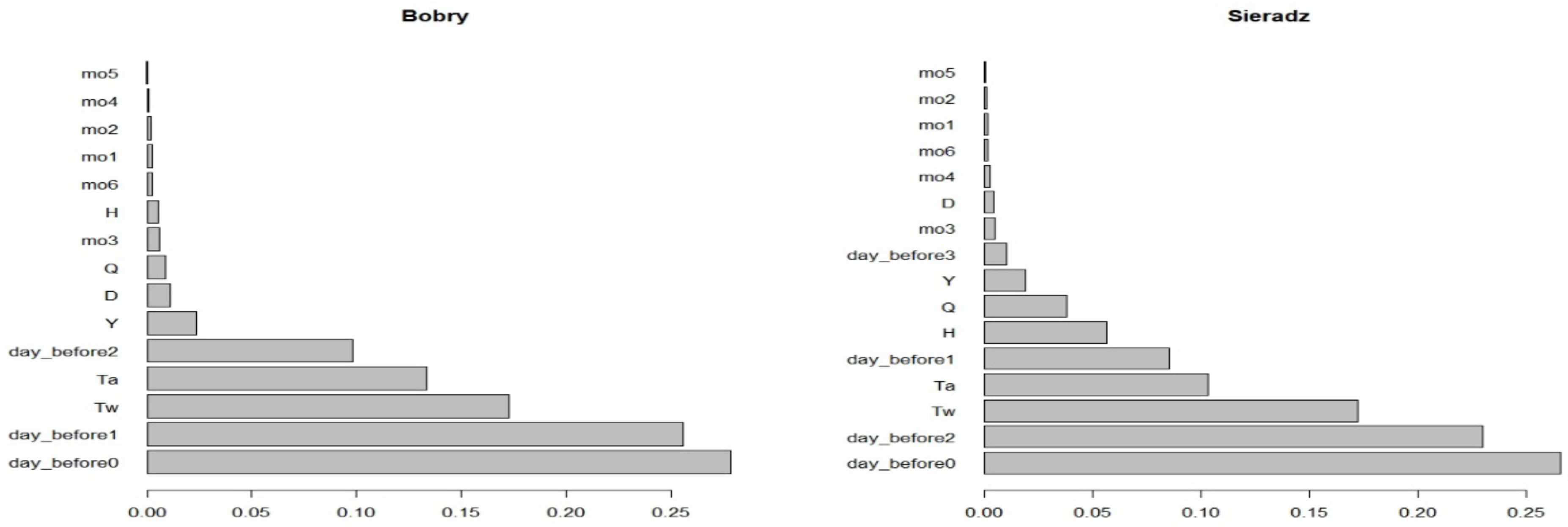
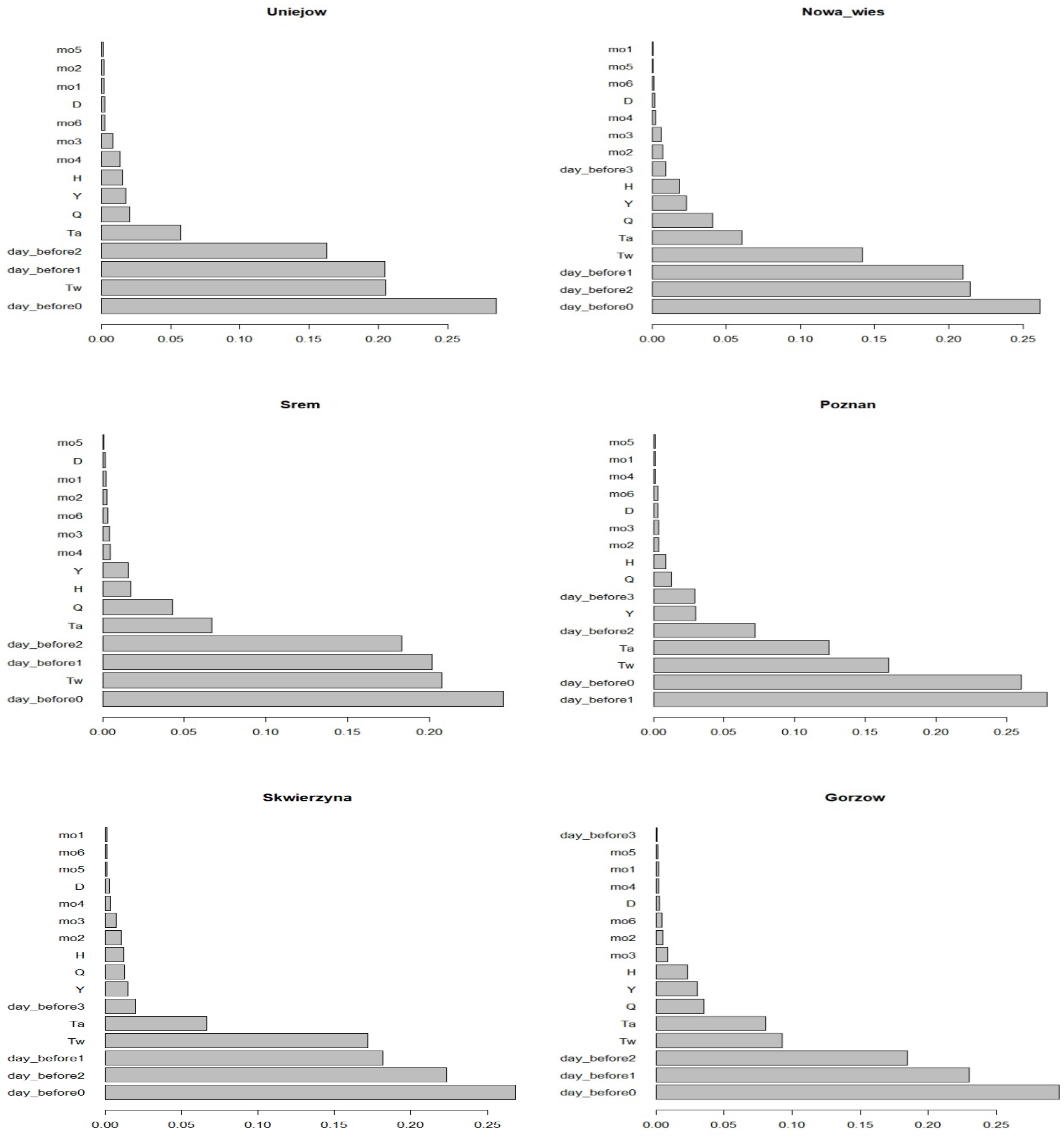
The use of XGBoost, as opposed to ANNs, made it possible to assess the importance of predictors in the model. The selected predictor variables were ranked according to the normalized reduction in model error, also known as “variable importance”. Figure 8 shows the most important predictor variables in the final model: water and air temperature, hydrological conditions (water level and river flow), and data for the “day before”, month, and year. The results of this analysis indicate that for each measuring station the most important predictor of ice phenomena is the type of ice phenomenon the day before the identification of a given event, with water temperature and air temperature coming next. In the case of the stations in Uniejow and Srem, water temperature is the second most important predictor of the occurrence of ice phenomena.

These results suggest that when looking for a balance between the complexity of the model and its predictive power, the two most important predictors for the occurrence of ice phenomena on the Warta River should be taken into account, i.e., the nature of the ice phenomenon on the day preceding the observation (especially for class 2 or class 1 events), and water temperature.

5. Discussion

5.1. Selection of Predictors as Input Variables

The predictive modeling of ice phenomena carried out on the example of the Warta River showed that the prediction of their occurrence in different phases and spatial locations gives different results. In this case, the prediction was a difficult process, mainly due to the complexity of interactions between hydroclimatic factors and thermal conditions that contribute to the occurrence of freezing.

In the research conducted on the Warta River, an important assumption was the selection of input variables that affect the accuracy of predictions in the neural network models and XGBoost. A set of daily data were used, these including thermal and hydrological variables, the type of ice phenomenon (group of phenomena) on the day preceding water gauge observations, and the month of their occurrence. The premises confirming the correctness of their choice are the results of studies of the ice regimes of rivers in Poland, including those conducted on the Vistula River [13,58], Oder River [59], on the rivers of the Baltic coastal zone [60,61], Bug River [62], and Warta River [46,63,64]. The selection of input variables significantly affects the performance of ANN models [7], however, it is often arbitrary [8].

5.2. The Most Important Predictor Variables in the Final Model

The results of the predictive models that we developed for the Warta River showed that all the input parameters (predictors) that were taken into account had some significance for the formation of ice phenomena from different classification groups. However, under the thermal conditions established for the reference period (research period 1984–2013), hydrological parameters—river flow and water level—were less important for the process of ice phenomena formation. The research established that ice phenomena occurred irregularly and periodically in the studied period and that the structure of freezing along the river course was diversified. The phenomena from class 1 were predominant, i.e., from the freezing phase of the river, represented by frazil ice and border ice, which is now a typical feature of the ice regime of most rivers in Poland [47].

The results of modeling confirmed that the most important predictors in the analyzed case were the nature of the phenomenon on the day preceding the observation (most often class 2 or class 1), as well as water temperature, and then air temperature (Figure 8). Graf [12] examined the dependencies of the trends of ice phenomena in the Noteć River, in western Poland (a tributary of the Warta River), on air and water temperature using regression models for count data and the Zero-Inflated Negative Binomial Model; results showed that the temperature values are the best predictors. In some locations, however, the model predicting the number of ice phenomena—taking into account the relationship with temperature—turned out to be statistically insignificant. Graf and Tomczyk [11] determined that for the Noteć River, a faster increase in accumulated sequences of negative air temperature contributes to an increase in the probability of a permanent ice cover, and the average degree day increase by one degree increases the chance of ice cover on the river in the range of 1.5–6.0% in different water gauges.

The period of intense changes in thermal conditions in the Warta catchment area, e.g., the cold period or sudden spring river supply, can be represented by changes in the models. However, it is also visible in the types of distributions illustrating the relationship between the classes of ice phenomena on the Warta River and hydrological factors and thermal conditions, which has been presented in the violin plots. The violin plots show diverse and complicated relations resulting from the differing variability of hydroclimatic factors and thermal conditions, which determines the nature of the distribution (Figure 5). Conditions conducive to the emergence of ice phenomena are not always the same in every location on the river, which is the result of local conditions, including, e.g., channel morphology and the influence of anthropic pressure.

5.3. The Performance of Predictive Models

The models performed promisingly in predicting the occurrence of ice phenomena on the Warta River, and this—in addition to their low demand for computational data resources, speed of operation, and ease of use—makes them particularly attractive. Further, it was found that the ANN approach served its purpose. By using more advanced and specialized network architectures (NN5, NN6), the ability to learn and predict the non-linear behavior of ice phenomena was increased for classes 2 and 3, which were characterized by a lower frequency of occurrence in the Warta River.

In ANN predictive modeling, the use of the sigmoidal function as an activation function for output layer neurons ensured that predictions obtained with the model would be the probabilities of occurrence of a given class, since this function maps real values to the range 0–1. As a result, models with 3, 4, 5, and 6 neurons in the hidden layer were developed, and this made it possible to compare their performance in predicting ice phenomena. Guo et al. [4], basing their work on the ANN theory, used the sigmoidal function as the activation function in the hidden layer for the forecasting of ice jams during river ice breakup. Their results were promising, as they predicted the annual occurrence of ice blockages with an accuracy of 85%, while the projected decay date with the projected ten-day period showed a maximum error of two days.

Concerning the prediction of class 1 and class 2 phenomena in the Warta River (permanent ice cover) and their non-occurrence, ANNs require further improvement, although present results indicate that they are comparable to the XGboost algorithm for predicting group 2 phenomena, i.e., permanent ice cover. The performance of the NN models and the XGBoost algorithm is also comparable for the different water gauge locations on the Warta River, although an overall better fit of XGBoost and NN4/NN5 models was observed for the upper course of the river; XGBoost and NN5/NN3 were most successful for the middle course, while NN models predominated for the lower course. The results of a comparison of both types of models in terms of their suitability for predicting ice phenomena on the Warta River showed a high accuracy of prediction for the XGBoost method, which has not been used on a larger scale in this regard so far.

XGBoost models variable interactions and handles the multi-linearity common to ecological datasets seamlessly [65]. Moreover, XGBoost works faster than many other gradient-increasing algorithms due to the regularization factor and the parallel computing functionality. One of the advantages of this method is its resistance to outliers, which eliminates the need to supplement missing data, and thus, in the case of the Warta River, it allows an increase in the efficiency of the prediction of a given phenomenon, even when eliminating outliers. The obtained results were considered satisfactory, which was confirmed by four model fit measures.

The comparison of results obtained for the Warta River with the ANN models used to predict ice phenomena on other rivers shows their considerable similarity. Most of the predictive and prognostic models developed confirm that the results of ice condition forecasts made with the use of ANNs are satisfactory and consistent with the measured data [37,66,67]. Moreover, the high accuracy of forecasts is indicated, which takes into account factors influencing the formation and disappearance of ice phenomena. Too many simplifications, as made in some models, may lower their prognostic accuracy and limit their usefulness for other rivers [36]. According to Massie [33], neural network classifiers, just like in the case of empirical methods, are most likely location-specific, but it is possible to transfer ANN models to other locations with minimal modifications. However, there are still no solutions for the prediction of phenomena in individual phases of their occurrence using the XGBoost algorithm. In Poland to date, models from the ANN group and the XGBoost algorithm have not been used to predict ice phenomena.

A review of the literature shows that numerous parameters are needed to support models developed for forecasting ice phenomena, most commonly ice jams and the resultant floods, but obtaining this data is sometimes difficult or even impossible. Despite the progress made in forecasting ice processes on rivers, this field still has great research potential; however, it also requires comprehensive observations, the collection and testing of data from stationary measurement networks, and direct field studies [8].

6. Conclusions

In the present study, MLPNN and XGBoost models were developed to forecast ice phenomena on the Warta River in Poland. The results obtained lead to the following conclusions:

(1)

Both the MLPNN and XGBoost models produced promising results for the forecasting of ice phenomena, which are presented using the four model fit measures.

(2)

For highly unbalanced classification problems, as in the case of the analyzed data, the “Balanced Accuracy” is particularly useful, since this statistic depends on both the level of correct prediction of a phenomenon and the level of prediction of the absence of a phenomenon.

(3)

The XGBoost turned out to be the best for predicting freeze-up (class 1) and ice cover (class 2 of ice phenomena), and at three water gauges its performance was comparable with that of the NN models, whereas breakup and ice deterioration (class 3) were best predicted by the NN5 model (at five water gauge stations). No dependence of the performance of individual models on the location of water gauges was observed.

(4)

The choice of input variables impacts the accuracy of the models developed. The nature of ice phenomenon on the day preceding the observation, as well as water and air temperature values, are important predictors, while river flow and water level were less important for the process of ice phenomena formation. This information was provided by the XGBoost algorithm.

(5)

The forecasting of ice phenomena is complicated due to the complex interactions between their determinants. This is confirmed by the types of distribution (unimodal, bimodal), illustrating the relationship between classes of phenomena on the river and hydroclimatic factors and thermal conditions.

The results of the research conducted here have important implications for forecasting ice phenomena, specifically as regards the application of XGBoost. Preliminary results seem to indicate that XGBoost, as an ensemble machine learning model, works well as a forecasting tool in hydrological research. Though the MLPNN and XGBoost models performed competently, there is still scope for further improvement through additional studies and the construction of hybrid models. Other factors influencing the occurrence of ice phenomena on rivers that would additionally help to improve the accuracy of these models should also be looked at (e.g., channel morphology, the accumulated degree days of frost and thaw, and the rates of change in water level and flow during the freeze-up and breakup periods). Since the present results concern only one river, future research will focus on applying models to rivers in different geographic locations and hydrological regimes to more accurately test the suitability and effectiveness of models.

References

- Magnuson, J.J.; Robertson, D.; Benson, B.; Wynne, R.; Livingstone, D.; Arai, T.; Assel, R.; Barry, R.; Card, V.; Kuusisto, E.; et al. Historical trends in lake and river ice cover in the northern hemisphere. Science 2000, 289, 1743–1746. [Google Scholar] [CrossRef] [PubMed] [Green Version]
- Hicks, F.; Beltaos, S. River Ice. In Cold Region Atmospheric and Hydrologic Studies. The Mackenzie GEWEX Experience; Woo, M., Ed.; Springer: Berlin/Heidelberg, Germany, 2008. [Google Scholar]
- Zhao, L. River Ice Breakup Forecasting Using Artificial Neural Networks and Fuzzy Logic Systems. Ph.D. Thesis, Department of Civil and Environmental Engineering, University of Alberta, Edmonton, AB, Canada, 2012. [Google Scholar]
- Guo, X.; Wang, T.; Fu, H.; Guo, Y.; Li, J. Ice-jam forecasting during river breakup based on neural network theory. J. Cold Reg. Eng. 2018, 32, 04018010. [Google Scholar] [CrossRef]
- Beltaos, S.; Prowse, T. River-ice hydrology in a shrinking cryosphere. Hydrol. Proc. 2009, 23, 122–144. [Google Scholar] [CrossRef]
- Lindenschmidt, K.-E.; Huokuna, M.; Burrell, B.C.; Beltaos, S. Lessons learned from past ice-jam floods concerning the challenges of flood mapping. Int. J. River Basin Manag. 2018, 16, 457–468. [Google Scholar] [CrossRef]
- Massie, D.D.; White, K.D.; Daly, S.F. Application of neural networks to predict ice jam occurrence. Cold Reg. Sci. Technol. 2002, 35, 115–122. [Google Scholar] [CrossRef]
- Madaeni, F.; Lhissou, R.; Chokmani, K.; Raymond, S.; Gauthier, Y. Ice jam formation, breakup and prediction methods based on hydroclimatic data using artificial intelligence: A review. Cold Reg. Sci. Technol. 2020, 174, 103032. [Google Scholar] [CrossRef]
- Nafziger, J.; She, Y.; Hicks, F. Anchor ice formation and release in small regulated and unregulated streams. J. Cold Reg. Sci. Technol. 2017, 141, 66–77. [Google Scholar] [CrossRef]
- Lindenschmidt, K.-E. RIVICE—A non-proprietary, open-source, one-dimensional river-ice and water-quality model. Water 2017, 9, 314. [Google Scholar] [CrossRef]
- Graf, R.; Tomczyk, A.M. The Impact of cumulative negative air temperature degree-days on the appearance of ice cover on a river in relation to atmospheric circulation. Atmosphere 2018, 9, 204. [Google Scholar] [CrossRef] [Green Version]
- Graf, R. Estimation of the dependence of ice phenomena trends on air and water temperature in river. Water 2020, 12, 3494. [Google Scholar] [CrossRef]
- Kolerski, T. Modeling of ice phenomena in the mouth of the Vistula River. Acta Geophys. 2014, 62, 893–914. [Google Scholar] [CrossRef]
- Shulyakovskii, L.G. Manual of Forecasting Ice-Formation for Rivers and Inland Lakes. Manual of Hydrological Forecasting No. 4; Translated from Russian, Israel Program for Scientific Translations; Central Forecasting Institute of USSR: Jerusalem, Israel, 1963. [Google Scholar]
- Uzuner, M.S.; Kennedy, J.F. Theoretical model of river ice jams. J. Hydraul. Eng. Div. 1976, 102, 1365–1383. [Google Scholar] [CrossRef]
- Yang, X.; Pavelsky, T.M.; Allen, G.H. The past and future of global river ice. Nature 2020, 577, 69–73. [Google Scholar] [CrossRef] [PubMed]
- Weber, F.; Nixon, D.; Hurley, J. Semi-automated classification of river ice types on the Peace River using RADARSAT-1 synthetic aperture radar (SAR) imagery. Can. J. Civil Eng. 2003, 30, 11–27. [Google Scholar] [CrossRef]
- Lindenschmidt, K.; Syrenne, G.; Harrison, R. Measuring ice thicknesses along the Red River in Canada using RADARSAT-2 satellite imagery. J. Water Resour. Prot. 2010, 2, 923–933. [Google Scholar] [CrossRef] [Green Version]
- Kolerski, T. Mathematical modeling of ice dynamics as a decision support tool in river engineering. Water 2018, 10, 1241. [Google Scholar] [CrossRef] [Green Version]
- Mahabir, C.; Hicks, F.; Fayek, A.R. Transferability of a neuro-fuzzy river ice jam flood forecasting model. Cold Reg. Sci. Technol. 2007, 48, 188–201. [Google Scholar] [CrossRef]
- White, K.D.; Daly, S.F. Predicting Ice Jams with Discriminant Function Analysis. In Proceedings of the ASME 2002 21st International Conference on Offshore Mechanics and Arctic Engineering, Oslo, Norway, 23–28 June 2002; Volume 3, pp. 683–690. [Google Scholar]
- Beltaos, S. Numerical modelling of ice-jam flooding on the Peace-Athabasca Delta. Hydrol. Proc. 2003, 17, 3685–3702. [Google Scholar] [CrossRef]
- Shen, H.T. Mathematical modelling of river ice processes. Cold Reg. Sci. Technol. 2010, 621, 3–13. [Google Scholar] [CrossRef]
- Wang, J.; Sui, J.; Guo, L.; Karney, B.W.; Jüpner, R. Forecast of water level and ice jam thickness using the back propagation neural network and support vector machine methods. Int. J. Environ. Sci. Technol. 2010, 7, 215–224. [Google Scholar] [CrossRef] [Green Version]
- Beltaos, S. Progress in the study and management of river ice jams. Cold Reg. Sci. Technol. 2008, 51, 2–19. [Google Scholar] [CrossRef]
- Lindenschmidt, K.-E.; Carstensen, D.; Fröhlich, W.; Hentschel, B.; Iwicki, S.; Kögel, K.; Kubicki, M.; Kundzewicz, Z.W.; Lauschke, C.; Łazarów, A.; et al. Development of an ice-jam flood forecasting system for the lower Oder River—Requirements for real-time predictions of water, ice and sediment transport. Water 2019, 11, 95. [Google Scholar] [CrossRef] [Green Version]
- Sutyrina, E.N. Prediction of spring ice phenomena on lakes and reservoirs using teleconnection indices. Limnol. Freshw. Biol. 2020, 4, 946–947. [Google Scholar] [CrossRef]
- Piotrowski, A.P.; Napiórkowski, M.J.; Napiórkowski, J.J.; Osuch, M. Comparing various artificial neural network types for water temperature prediction in rivers. J. Hydrol. 2015, 529, 302–315. [Google Scholar] [CrossRef]
- Graf, R.; Zhu, S.; Sivakumar, B. Forecasting river water temperature time series using a wavelet–neural network hybrid modelling approach. J. Hydrol. 2019, 578, 124115. [Google Scholar] [CrossRef]
- Zhu, S.; Heddam, S.; Nyarko, E.K.; Hadzima-Nyarko, M.; Piccolroaz, S.; Wu, S. Modeling daily water temperature for rivers: Comparison between adaptive neurofuzzy inference systems and artificial neural networks models. Environ. Sci. Pollut. Res. 2019, 26, 402–420. [Google Scholar] [CrossRef]
- Morse, B.; Hessami, M.; Bourel, C. Mapping environmental conditions in the St. Lawrence River onto ice parameters using artificial neural networks to predict ice jams. Can. J. Civ. Eng. 2003, 30, 758–765. [Google Scholar] [CrossRef]
- Wang, T.; Yang, K.L.; Guo, Y.X. Application of artificial neural networks to forecasting ice conditions of the Yellow River in the Inner Mongolia reach. J. Hydrol. Eng. 2008, 13, 811–816. [Google Scholar]
- Massie, D.D. Neural-Network Fundamentals for Scientists and Engineers. In Proceedings of the Conference on Efficiency, Costs, Optimization, Simulation and Environmental Impact of Energy Systems (ECOS 01), Istanbul, Turkey, 4–6 July 2001. [Google Scholar]
- Chokmani, K.; Khalil, B.; Ouarda, T.B.M.J.; Bourdages, R. Estimation of river ice thickness using artificial neural networks. In Proceedings of the 14th Workshop Hydraulics Ice Covered Rivers, Quebec, QC, Canada, 19–22 June 2007; CGU HS/CRIPE: Quebec, QC, Canada, 2007. [Google Scholar]
- Hu, J.; Liu, L.; Huang, Z.; You, Y.; Rao, S. Ice Breakup Date Forecast with Hybrid Artificial Neural Networks. In Proceedings of the 4th International Conference on Natural Computation, ICNC, Jinan, China, 25–27 August 2007; Volume 2, pp. 414–418. [Google Scholar]
- Chen, S.Y.; Ji, H.L. Fuzzy optimization neural network approach for ice forecast in the Inner Mongolia reach of the Yellow River. Hydrol. Sci. J. 2005, 50, 319–330. [Google Scholar]
- Yan, Q.; Ding, M. Using Dynamic Fuzzy Neural Networks Approach to Predict Ice Formation. In Proceedings of the 2011 MSEC International Conference on Multimedia, Software Engineering and Computing, Wuhan, China, 26–27 November 2011; Jin, D., Lin, S., Eds.; Advances in Multimedia, Software Engineering and Computing Vol.1. Springer: Berlin/Heidelberg, Germany, 2011; Volume 128. [Google Scholar]
- Liu, H.; Jiang, Q.; Ma, Y.; Yang, Q.; Shi, P.; Zhang, S.; Tan, Y.; Xi, J.; Zhang, Y.; Liu, B.; et al. Object-Based Multigrained Cascade Forest Method For Wetland Classification Using Sentinel-2 and radarsat-2 imagery. Water 2022, 14, 82. [Google Scholar] [CrossRef]
- Shin, Y.; Kim, T.; Hong, S.; Lee, S.; Lee, E.; Hong, S.; Lee, C.; Kim, T.; Park, M.S.; Park, J.; et al. Prediction of chlorophyll-a concentrations in the Nakdong River using machine learning methods. Water 2020, 12, 1822. [Google Scholar] [CrossRef]
- Flach, P.A. Machine Learning: The Art and Science of Algorithms that Make Sense of Data; Cambridge University Press: Cambridge, UK, 2012. [Google Scholar]
- Prowse, T.D.; Bonsal, B.R. Historical trends in river-ice break-up: A review. Nordic Hydrol. 2004, 35, 281–293. [Google Scholar] [CrossRef]
- Zounemat-Kermani, M.; Batelaan, O.; Fadaee, M.; Hinkelmann, R. Ensemble machine learning paradigms in hydrology: A review. J. Hydrol. 2021, 598, 126266. [Google Scholar] [CrossRef]
- Graf, R.; Aghelpour, P. Daily river water temperature prediction: A comparison between neural network and stochastic techniques. Atmosphere 2021, 12, 1154. [Google Scholar] [CrossRef]
- Woś, A. The Climate of Poland in the Second Half of the 20th Century; Scientific Publishing House UAM: Poznan, Poland, 2010; 490p. (In Polish) [Google Scholar]
- Wrzesiński, D.; Perz, A. The features of the runoff regime in the basin of the Warta River. Bad. Fizjogr. R. VII Ser. A Geogr. Fiz. 2016, A67, 289–304. (In Polish) [Google Scholar]
- Graf, R.; Łukaszewicz, J.T.; Jawgiel, K. The analysis of the structure and duration of ice phenomena on the Warta River in relation to thermic conditions in the years 1991–2010. Woda-Sr.-Obsz. Wiej. 2018, 18, 5–28. (In Polish) [Google Scholar]
- Pawłowski, B.; Gorączko, M.; Szczerbińska, A. Ice Phenomena on the Rivers of Poland. In Hydrology of the Poland; Jokiel, P., Marszelewski, W., Pociask-Karteczka, J., Eds.; PWN: Warsaw, Poland, 2017; pp. 195–200. (In Polish) [Google Scholar]
- Graf, R.; Wrzesiński, D. Detecting patterns of changes in river water temperature in Poland. Water 2020, 12, 1327. [Google Scholar] [CrossRef]
- Lan, T.; Lin, K.; Tan, X.; Xu, C.-Y.; Chen, X. Dynamics of hydrological model parameters: Calibration and Reliability. Hydrol. Earth Syst. Sci. 2020, 24, 1347–1366. [Google Scholar] [CrossRef] [Green Version]
- Hintze, J.L.; Nelson, R.D. Violin plots: A box plot-density trace synergism. Am. Stat. 1998, 52, 181–184. [Google Scholar]
- Brownlee, J. Train-Test Split for Evaluating Machine Learning Algorithms. 2020. Available online: https://machinelearningmastery.com/train-test-split-for-evaluating-machine-learning-algorithms (accessed on 15 September 2021).
- Fritsch, S.; Guenther, F.; Wright, M.N. “Neuralnet: Training of Neural Networks.” R package version 1.44.2. 2019. Available online: https://CRAN.R-project.org/package=neuralnet (accessed on 22 November 2021).
- Riedmiller, M. Advanced supervised learning in multi-layer perceptrons—From backpropagation to adaptive learning algorithms. Comput. Stand. Interfaces 1994, 16, 265–278. [Google Scholar] [CrossRef]
- Chen, T.; He, T.; Benesty, M.; Khotilovich, V.; Tang, Y.; Cho, H.; Chen, K.; Mitchell, R.; Cano, I.; Zhou, T.; et al. Xgboost: Extreme Gradient Boosting. 2020. Available online: https://cran.r-project.org/package=xgboost (accessed on 10 July 2021).
- Loong, T.W. Understanding sensitivity and specificity with the right side of the brain. BMJ 2003, 327, 716–719. [Google Scholar] [CrossRef] [PubMed]
- Parikh, R.; Mathai, A.; Parikh, S.; Chandra Sekhar, G.; Thomas, R. Understanding and using sensitivity, specificity and predictive values. Indian J. Ophthalmol. 2008, 56, 45–50. [Google Scholar] [CrossRef] [PubMed]
- R Core Team, R. A Language and Environment for Statistical Computing; R Foundation for Statistical Computing: Vienna, Austria, 2019; Available online: http://www.R-project.org (accessed on 15 July 2021).
- Pawłowski, B. Course of Ice Phenomena on the Lower Vistula River in 1960–2014; Nicholas Copernicus University Toruń: Torun, Poland, 2017. (In Polish) [Google Scholar]
- Marszelewski, W.; Pawłowski, W. Long-term changes in the course of ice phenomena on the oder river along the Polish–German border. Water Resour. Manag. 2019, 33, 5107–5120. [Google Scholar] [CrossRef]
- Ptak, M.; Choiński, A. Ice phenomena in rivers of the coastal zone (southern Baltic) in the years 1956–2015. Baltic Coastal Zone. J. Ecol. Prot. Coastline 2016, 20, 73–83. [Google Scholar]
- Łukaszewicz, J.T.; Graf, R. The variability of ice phenomena on the rivers of the Baltic coastal zone in the Northern Poland. J. Hydrol. Hydromech. 2020, 68, 38–50. [Google Scholar] [CrossRef] [Green Version]
- Bączyk, A.; Suchożebrski, J. Variability of ice phenomena on the Bug River (1903–2012). Inżynieria Ekol. 2018, 49, 136–142. (In Polish) [Google Scholar] [CrossRef] [Green Version]
- Gorączko, M.; Pawłowski, B. Changing of ice phenomena on Warta River in vicinity of Uniejów. Biul. Uniejowski 2014, 3, 23–33. (In Polish) [Google Scholar]
- Kornaś, M. Ice phenomena in the Warta River in Poznań in 1961–2010. Quaest. Geogr. 2014, 33, 51–59. [Google Scholar] [CrossRef] [Green Version]
- Smith, E.H. Using extreme gradient boosting (XGBoost) to evaluate the importance of a suite of environmental variables and to predict recruitment of young-of-the-year spotted seatrout in Florida. bioRxiv 2019, 543181. [Google Scholar] [CrossRef]
- Wang, Z.; Li, C. River Ice Forecasting Based on Genetic Neural Network. In Proceedings of the International Conference on Information Engineering and Computer Science (ICIECS2009), Wuhan, China, 19–20 December 2009; pp. 1–4. [Google Scholar]
- Li, S.; Qin, J.; He, M.; Paoli, R. Fast evaluation of aircraft icing severity using machine learning based on XGBoost. Aerospace 2020, 7, 36. [Google Scholar] [CrossRef] [Green Version]
Figure 1.
Study area and the locations of water gauges and meteorological stations of the Institute of Meteorology and Water Management—National Research Institute (IMGW-PIB, Warsaw, Poland).
Figure 2.
Stages of research activities.
Figure 3.
Feed-forward multilayer perceptron architecture.
Figure 4.
A general architecture for XGBoost.
Figure 5.
Probability of occurrence of ice phenomena (classes 1–3 and none) as a function of the month for the water gauge stations on the Warta River. Note: Water gauge stations are labeled in the order (a–h), according to their location on the river (from upper to lower course).
Figure 6.
Probability of the order of occurrence of ice phenomena classes (none, C1, C2, C3) as a function of the ice phenomenon of the previous day for the water gauge stations on the Warta River. Note: Water gauge stations are labeled in the order (a–h), according to their location on the river (from upper to lower course).
Figure 7.
Distributions of the relationship between classes of ice phenomena (none, C1, C2, C3) and air and water temperatures (Ta, Tw), the water level (H), and river flow (Q).
Figure 8.
Relative importance of predictors in the XGBoost model (profit values).