Flood Extent Mapping from Time-Series SAR Images Based on Texture Analysis and Data Fusion


1
Imaging, Vision and Artificial Intelligence Laboratory, Automated Manufacturing Engineering Department, École de Technologie Supérieure, Université du Québec, 1100 Rue Notre-Dame Ouest, Montreal, H3C 1K3 QC, Canada
2
Computer Science Department, Faculty of Mathematical, Physical and Natural Sciences of Tunis, University of Tunis El Manar, 1068 Tunis, Tunisia
3
Computer Research Institute of Montreal, Montreal, H3N 1M3 QC, Canada
*
Author to whom correspondence should be addressed.
Remote Sens. 2018, 10(2), 237; https://0-doi-org.brum.beds.ac.uk/10.3390/rs10020237
Submission received: 7 November 2017
/
Revised: 26 January 2018
/
Accepted: 30 January 2018
/
Published: 4 February 2018
(This article belongs to the Special Issue Analysis of Multi-temporal Remote Sensing Images)
Abstract
:Nowadays, satellite images are considered as one of the most relevant sources of information in the context of major disasters management. Their availability in extreme weather conditions and their ability to cover wide geographic areas make them an indispensable tool toward an effective disaster response. Among the various available sensors, Synthetic Aperture Radar (SAR) is distinguished in the context of flood management by its ability to penetrate cloud cover and its robustness to unfavourable weather conditions. This work aims at developing a new technique for flooded areas extraction from high resolution time-series SAR images. The proposed approach is mainly based on three steps: first, homogeneous regions characterizing water surfaces are extracted from each SAR image using a local texture descriptor. Then, mathematical morphology is applied to filter tiny artifacts and small homogeneous areas present in the image. And finally, spatial and radiometric information embedded in each pixel are extracted and are fused with the same pixel information but from another image to decide if the current pixel belongs to a flooded region. In order to assess the performance of the proposed algorithm, our methodology was applied to time-series images acquired before and during three different flooding events: (1) Richelieu River and lake Champlain floods, Quebec, Canada in 2011; (2) Evros River floods, Greece in 2014 and (3) Western and southwestern of Iran floods in 2016. Experiments show that our approach gives very promising results compared to existing techniques.

1. Introduction
Regardless of whether they originate from the overflow of water bodies such as lakes or rivers, or from the melting snow during spring, floods share in common their devastating impact on human lives, environment and infrastructure. And despite various efforts to reduce their socio-economic and financial impacts, these initiatives remain insufficient given the constant increase in the frequency of these phenomena due to climate changes affecting our planet. In this context, remote sensing data has repeatedly shown its interest and usefulness during the various phases of flood management process [1,2,3] by providing an overview of the situation on the ground without direct contact with the flooded area and by allowing the decision makers to follow the water extent during the disaster. Hence the interest of developing new techniques to precisely delimit the extent of flooded areas based on high-resolution satellite images made increasingly available. In the literature, both SAR and optical images have been used to identify pixels associated with the flooded areas. It is obvious that identifying floods from optical images is easier than extracting them from SAR images because of the particular radiometric response that characterizes water surfaces. Techniques such as classification [4], segmentation [5] and fusion [6] have been successfully applied to extract floods from optical images. However, the use of this type of data is conditioned by the absence of a cloud cover during the flooding which can occlude the mapped scene and complicates the analysis of the collected data. Unlike optical data, SAR data have been widely used to extract floods as it has the advantages of penetrating through the cloud cover and the possibility of mapping the affected region at any time of the day and night [7]. The availability of these images has prompted worldwide researchers to propose new approaches allowing better exploitation of these data and minimizing the execution time of existing algorithms so that they meet the requirements in terms of rapid response and effective management.
Based on the thresholding of SAR backscattering value, several works have been proposed to solve the problem of flood extraction. They were mainly based on the assumption that the backscatter values of the flooded area in SAR images are very low, and therefore, it is sufficient to select pixels that are below a given threshold value to identify the affected areas. While it’s a simple technique and one of the first used in computer vision, it remains the most common and efficient way to identify flooded areas [8]. In [9], an automatic near-real time flood detection approach combining histogram thresholding and segmentation-based classification is described. The proposed technique apply a global thresholding integrated into a split-based approach in order to achieve a multiscale analysis of the input SAR image and extract flooded areas. Nakmuenwai et al. [8] use multi-temporal dual-polarized RADARSAT-2 images to classify water areas by means of a clustering-based thresholding technique. Their idea consists of selecting specific water references throughout the study area to estimate local threshold values and then averages them by an area weight to obtain the threshold value for the entire area. Obtained results are very promising, nevertheless non-water objects characterized by smooth surfaces such as roads and runways are classified as water surfaces. Other works have also been based on SAR backscatter value thresholding in order to delimit the flooding extent [10,11,12], however, the choice of the appropriate value of the flood separating threshold is very challenging and depends on many factors such as wavelength, incidence angle and dielectric properties of the target surface.
Change detection techniques have been widely applied in the literature to solve the problem of flooded areas extraction from SAR images [13,14,15,16,17]. The use of these families of approaches was mainly motivated by the availability of archive images that serve as a reference to identify changes that affect the area of interest. An enhanced version of M1 and M1a change detection algorithms described in [9] termed M2b is introduced in [13]. While M1 only considers a single SAR flood image to extract pixels corresponding to open water via image thresholding and region growing algorithm, M2b adds change detection information with respect to a non-flood reference image to improve the algorithm’s performance. This enables the identification of non-target areas such as shadow that systematically behave as specular reflectors from images acquired during dry conditions. Traditional change detection methods such as log-ratio were applied to identify changed regions from flood images. In [14], multi-temporal SAR data are employed to compute a polarimetric log-ratio used to highlight changes in terms of magnitude and direction. This information is, thereafter, analyzed in order to separate non-changed and changed samples. An extension of the curvelet-based change detection approach to polarimetric SAR data for monitoring flooded vegetation is proposed in [15]. First, the Freeman–Durden decomposition is used to classify the SAR backscatter into double bounce, surface scattering and volume scattering. Then, a change detection algorithm is applied to all three channels separately based on the following hypothesis: the presence of water due to flooding is reflected by an equal increase in all three channels, whereas the change of a special scattering event only appears in the dedicated scattering mechanism intensity. Image rationing is also used in [16] combined with Bayesian unsupervised minimum-error thresholding algorithm to extract changes generated by floods from medium and high-resolution X-band SAR images. In this work, a Generalized Gamma distribution (GD) is chosen to accurately model the statistics of SAR amplitudes at moderate to high-resolution images. One of the major drawbacks of these change detection-based techniques is that it is complex to precisely determine the nature of the change in SAR image and to decide whether it is due to the disaster impact or originates from other events. This problem becomes more complicated if we are comparing images acquired using different polarimetric configuration where the backscatter response of the same object can appear very different from one image to another without a real change on the ground [17].
Some known classifiers such as Support Vector Machine (SVM) and Artificiel Neural Network (ANN) were used in [18,19,20] to classify the input image into flooded and non-flooded areas based on features reflecting radiometric, textural and spatial properties of SAR images. These classifiers aim at estimating the class of a region contained in the input image based on its characteristics and backscatter properties. Sakakun [18] propose a neural network-based approach to map floods from ERS-2 and RADARSAT-1 satellite images. He applies a self organized Kohonen’s maps (SOMs) as it can be trained using unsupervised learning to produce a map that preserves the topological properties of the input space. SVM and particle filter (PF) were combined in [19] to identify the extent of the 2001 Thailand flood. The proposed technique is mainly based on estimating SVM training model parameters using the observation system of the PF in order to define an appropriate value for these latter. Pradhan et al. [20] apply an iterative self-organizing data analysis technique (ISODATA) to classify flooded areas from TerraSAR-X satellite images acquired during a flood event and compare the obtained result with water bodies detected from Multispectrale Landsat images. The described method works well in open areas but the accuracy is dramatically reduced in urban areas. Several classifiers such as SVMs have shown their effectiveness in flooded image classification compared to neural networks especially if applied to a small database, however, the performance of these classifiers highly rely on the quality of the extracted features.
Several works in the literature have shown the potential of object-based image analysis (OBIA) applied to SAR image [21,22,23]. They concluded that speckle noise characterizing SAR images reinforces the choice of an OBIA approach since single pixel value do not only represent backscattering value but also correspond to the coherent interference of waves reflected from many elementary scatterers within a resolution cell. This is particularly true if we are dealing with the problem of flood extent analysis where it is extremely difficult to decide, based on information contained in a single pixel, whether or not it belongs to a flooded area. In [21], a novel hybrid change detection (HCD) combining object-based change detection (OBCD) and pixel-based change detection (PBCD) is introduced. The proposed technique benefits from the complementary information provided by an OBCD and a PBCD approaches to improve the performance of flood detection from multitemporal SAR images. Arnesen et al. [22] introduce a hierarchical object-based classification approach to monitor the Amazon River large seasonal variations in water level and flood extent. Implemented by means of a data mining algorithm, the proposed technique includes auxiliary information such as water level records, field photography, optical satellite images and topographic data. They demonstrate the potential of applying their technique to wide swath L-band SAR images for monitoring flood extent. A comparative study conducted by the German Remote Sensing Data Center (DFD) of the German Aerospace Center (DLR) and including four operational SAR-based water and flood detection approaches is described in [23]. One of the introduced techniques termed Rapid Mapping of Flooding (RaMaFlood) gives very promising results compared to the other approaches but the need for the intervention of a human interpreter makes it unsuitable for major flooding events.
Our approach differs from existing techniques by its low sensitivity to speckle noise characterizing SAR images due to the use of kernel-based texture measurement robust to local texture variation. Also, to the best of our knowledge, a texture measurement is applied for the first time to extract floods extent from high resolution radar images. Another contribution of this work consists of introducing a novel fusion method based on the combination of spatial and radiometric information contained in each pixel and also the management of their uncertainty and contradiction using Dempster-Shafer theory applied to time-series SAR images.
The remainder of this paper is organized as follows: Section 2 describes the study areas and the SAR data used in this work to validate the proposed approach. Section 3 introduces our flood extent extraction algorithm and recalls the main concepts of the applied Structural Feature Set texture measurement, morphological path openings and Dempster-Shafer based fusion theory. Section 4 and Section 5 discuss the results obtained by applying our technique to three different sites and compares them with existing approach dealing with the same problematic. And finally, Section 6 concludes.
2. Study Areas and Available Data
2.1. Study Areas
In order to evaluate the robustness and the effectiveness of our approach dedicated to flood damage extraction from time-series SAR images, flood events that hit three different sites were chosen in this study as shown in Figure 1. The first site described in Figure 1a covers a part of the Richelieu River located south of the province of Quebec, Canada. This river rises at Lake Champlain, from which it flows to the north of the province and empties into the St. Lawrence River. We are particularly interested in floods that have occurred from April to June 2011 because it was considered as one of the most devastating weather events that hit Canada in 2011 as they had caused significant damage to 6000 hectares of farmland and affected nearly 3000 homes and cottages [24]. The second site shown in Figure 1b refers to the Evros River located in Greece and marks its eastern border with Turkey. It is the second largest river in Eastern Europe after the Danube and it has its origin in the Rila Mountains in Western Bulgaria, flowing southeast between the Balkan and Rhodope Mountains, past Plovdiv and Parvomay to Edirne, Turkey. East of Svilengrad, Bulgaria, the river flows eastwards, forming the border between Bulgaria and Greece, and then between Turkey and Greece [25]. Through the years, catastrophic flood events have occurred along this river, however, in this work we are focusing on floods that have occurred from November to December 2014 because of the event extent, the devastating impact and the availability of Sentinel-1 images before and during the disaster. The last site associated to Figure 1c covers a part of the Dez River located in the southwestern part of Iran and formed by the joining of the Caesar and Bakhtiary Rivers [26]. This river is very important for the province of Khuzestan as it supplies the water demands of 16 cities, several villages, thousands hectares of agricultural lands, and several hydropower plants [27]. We are particularly interested in floods that have occurred from March to April 2016 mainly caused by heavy rain and hit at least four provinces of Kermanshah, Ilam, Lorestan and Khuzestan. This disaster quickly spread to reach 126 cities in western and southwestern Iran causing serious damage to their infrastructure and historical sites. These events can be considered as extreme disasters given the magnitude of the disaster and for the large amount of satellite data made available during the floods.
2.2. Available Data
The RADARSAT-2 and Sentinel-1 SAR images collected over the three study sites are listed in Table 1. Images used to assess the extent of Richelieu River flooding were obtained as part of the initiative Science and Operational Applications Research - Education (SOAR-E) (http://www.asc-csa.gc.ca/eng/ao/2008-soar-e.asp) supported by the Canadian Space Agency (CSA) and Canada Centre for Remote Sensing which aims at developing innovative RADARSAT-2-based techniques and promoting the use of synthetic aperture radar (SAR) remote sensing. All available RADARSAT-2 images are 8 m of resolution using the fine quad-polarization mode in single-look complex form (SLC). Sentinel-1 images of sites 2 and 3 are used to study the two other flooding events. These images were freely available through the Copernicus Open Access Hub (https://scihub.copernicus.eu/) which acts as access point for all Sentinel missions with access to the interactive graphical user interface. Sentinel-1 Interferometric Wide swath mode (IW) was used to create images characterized by a large swath width (250 km) and a moderate resolution of 12 m.
The SAR images available in this study have already been pre-processed to provide usable high-level products from raw satellite data, however, other radiometric and geometric corrections such as radiometric calibration, range doppler terrain correction based on the Shuttle Radar Topography Mission and images coregistration are necessary in order to reduce distortion effects and prepare the data for the application of our technique. Also, the Sentinel-1 IW mode used to acquire images from sites 2 and 3 captures for each image three sub-swaths using Terrain Observation with Progressive Scans SAR (TOPSAR) technique [28]. In order to join all burst data into a single image of the scene of interest, TOPSAR deburst operator is applied.
3. Proposed Approach
3.1. Overview
We propose a new technique capable of extracting flooded areas and monitoring their extent from time-series SAR images. The proposed approach should also be able to identify the initial surface of the studied water body in order to delimit the flooded area that has emerged as a result of the disaster impact. In case of calm water bodies, specular reflection is expected to be dominant because most of the incident radar energy is reflected away which explains their dark radiometry and homogeneous texture. This is generally true unless the water surface becomes rough due to local winds as is the case of floods. In such situations, it is rather the multiplicative model that becomes valid for an L look intensity image, where the intensity standard deviation is proportional to the mean , however, these variations remain local and the overall texture can still be considered as homogeneous. In light of these findings, we based our reasoning on the analysis of homogeneity as a discriminant feature to characterize water bodies and to distinguish them from other objects in SAR images. Many homogeneity measurements were proposed in the literature mainly based on standard deviation computation or co-occurrence matrix analysis, however, these techniques remain very sensitive to the presence of small artifacts and noises in the analyzed region. In this work, an original application of texture analysis to extract water bodies and flooded areas from SAR images is introduced. Our texture measurement provides the degree of homogeneity associated to each pixel of the analyzed window, which allows to distinguish the target classes from the rest of the image.
As shown in Figure 2, the proposed approach is mainly based on three phases. First, the Structural Feature Set (SFS) texture measurement is applied to extract homogeneous areas characterizing not only water bodies but also other objects such as roads, agricultural fields and highways. As our objects of interest can have different shapes, we opted for the standard deviation (SD) variant of this measurement able to identify different patterns including narrow and elongated ones. We recall that at this level of the methodology our goal is not to extract water bodies in particular, but all the homogeneous areas contained in the input SAR images. This texture measurement is a pixel-wise descriptor, therefore it provides a homogeneity value associated to each pixel of the image. However, its computation from an analysis window adds more robustness to this descriptor and decreases the influence of speckle and local winds on the homogeneity computation. A morphological opening path operator is used, thereafter, with the aim to remove small homogeneous objects and noise resulting from the application of the previous step. The idea consists in filtering more information from the pre-flooding image, as it contains only the surface of a river or a lake, and filter less information from the post-flooding images as it contains objects of the pre-flooding image, in addition to flooded areas characterized by a smaller size. Regarding the choice of the structuring element, we were mainly guided by the shape of our objects of interest. Therefore, as we seek to retain both linear structures such as rivers and arbitrary ones such as lakes and flooded areas, a structuring element in the form of a path is applied. The last step consists in fusing the resulting images in pairs to determine the flooding extent as a function of time. This operation is quite difficult in our case because unlike traditional change detection problems where binary images are processed, values of our homogeneity measurement are in the range [0, 255]. To overcome this problem, we used the Dempster Shafer theory which represents a very powerful mathematical tool for combining imprecise, uncertain and conflicting sources of information. This theory was applied in this work at two levels: first, to combine a spatial-based and a radiometric-based sources of information resulting from the application of morphological profile and evidential C-means and second, to fuse mass function obtained from each image using the multidimensional evidential reasoning. The initial surface of the river or of the lake can be identified directly by applying the first two steps on the pre-flooding image, as we have already demonstrated in previous works [29,30].
For the sake of simplification, we will, in what follows, present the intermediate results obtained by applying each step of our algorithm to the two input images shown in Figure 3a,b corresponding to Richelieu River pre- and post flooding SAR images. However, the proposed method was mainly designed to process time-series SAR images and can be easily generalized to handle multiple input images.
3.2. Texture Extraction Using a Structural Feature Set (SFS)
In previous works, we successfully applied the SFS texture measurement to extract homogeneous areas such as road networks from optical images [31,32], and water bodies from SAR images [29,30]. This descriptor has shown very promising results applied to optical images characterized by the presence of various artifacts arising from the use of high spatial resolution and SAR images affected by speckle noise. In general, whether for the extraction of water bodies or the identification of other structures in SAR imagery, the application of a pre-processing step is generally required. Most of the methods proposed for thresholding, contour extraction or texture analysis are very sensitive to noise in SAR images. In this work, a pre-processing step is not necessary, as our image analysis technique is mainly based on the search for homogeneous objects (homogeneous in the sense of a stationnary texture and reflectivity) in the flood extent identification process. In SAR images, the water surfaces are characterized by a high degree of homogeneity, which distinguishes them from the other land use classes in the image. This characteristic has been taken into account in the choice of the first step of our algorithm, which consists in applying the texture measurement of all structural characteristics (SFS) to extract homogeneous and elongated zones. The idea consists in using local statistics to decide whether a pixel belongs to a homogeneous zone while minimizing the influence of outlier pixels representing in our case local winds.
The so-called structural feature set (SFS) is a set of measurements used to extract the statistical features of a direction-lines histogram [33,34]. We introduce some concepts to define these measurements: we first define direction lines as a set of equally-spaced lines through a central pixel. For a given direction, the radiometric difference between a pixel and its central pixel is measured to determine whether this pixel lies in a homogeneous area around the central pixel. The homogeneity measurement is defined as:
where is the homogeneity measurement of the ith direction between the central pixel and its surrounding pixel, and , which represent the radiometric values of the surrounding pixel and the central pixel, respectively. The ith direction line is extended if the following conditions are met:
- is less than a predefined threshold .
- The total number of pixels in this direction line is less than another threshold .
Next, we define the length of all of the direction lines for a given pixel:
in which represent the row and the column of the pixel at one end, and the row and the column, respectively, of the pixel at the other end. We can thus define the direction-line histogram associated with a central pixel as:
where I represents the image, c the central pixel and D the set of all of the direction lines. The SFS was associated with six texture measurements calculated from a histogram in [34]. In our work, the ratio and the standard deviation (SD) measurements can be used to characterize the arbitrary shapes of flooded areas, however, it is preferable to apply the SD variant able to identify different patterns including narrow and elongated ones such as rivers and roads contained in the pre-flooding image. The SFS-SD is illustrated as follows:
where denotes the standard deviation calculated from the direction-line histogram, and represents the mean value of the histogram, defined as:
The aim of this step is to identify all potential candidates, consequently, not only target objects such as lakes, rivers and flooded areas will be retained, but also roads, agricultural areas and some small artifacts. Distinguishing target objects from among these structures will be addressed in the next phase. Also the choice of the two parameters and will be examined in the discussion.
Results obtained by applying the SFS-SD on the two input images are shown in Figure 4. As we can notice, the used descriptor provides relevant information on the degree of homogeneity of each pixel of the image based on the analysis of its immediate neighbours. Therefore, a pixel belonging to a water body will appear brighter than a pixel associated to a flooded area, which in turn will appear brighter than speckle and small artifacts. The next step will be dedicated to the removal of non-target pixels by means of mathematical morphology.
3.3. Non-Target Objects Removal
The application of the previous step allowed to retain objects presenting homogeneous texture response such as rivers, lakes and flooded areas. However, other structures such as agricultural fields, small artifacts and noise have also been retained because of their very similar texture. Indeed, it is very difficult to decide based only on local information if an object is of sufficient size to be considered as an object of interest or not. In order to remedy this problem, we apply an efficient image denoising approach mainly based on mathematical morphology that allows irrelevant information to be filtered out while keeping desired object’s structure. The main challenge in the application of this family of approaches resides in the choice of the structuring element’s shape and size which depend on the target application and the dimensions of the object of interest. In our case, this choice is very complicated because our objects of interest are very varied and do not have a unique shape. If we take the example of rivers, these structures are characterized by a very small width compared to their length, therefore a structuring element with dimensions greater than the river’s width will remove it completely. On the other hand, choosing a too-small structuring element will have no effect on the noise present in the image. This leads us to use structural elements in the form of paths, as described in [35,36,37], able to extract arbitrary shapes including linear structures and objects that present local linearity. We will briefly introduce the theory behind path opening and closing. For simplicity, the concept of binary image is employed in the following definitions, but the theory can be generalized to cover grayscale images as well.
Let be a binary image, in which we first define the following relationship: , where x and y are two pixels of and the symbol ‘↦’ denotes the adjacency relationship between those two pixels and means that there is an edge going from x to y. This also means that x is a predecessor of y and y is a successor of x. Based on this notation, we define the dilation by:
In other words, the dilation of a subset comprises all those points that have a predecessor in X. The L-tuple is called a -path of length L if , or equivalently, if:
Given a path a in , the set of its elements is denoted with . The set of all -paths of length L is denoted as . The set of -paths of length L contained in a subset X of is denoted by :
Finally, we define the opening or the path-opening as the union of all paths of length L in X such that:
In the same way, we define the path-closing by simply exchanging the foreground and background. However, in this work, we will only use the path-opening operator as our object of interest is brighter than the rest of the image. This operator is mainly dependent on one parameter, termed and is used to remove objects with lengths above this predefined threshold. In order to choose its appropriate values, we were based on the following heuristics: (1) From the pre-flooding image, we want to keep only large water bodies, thus, a high value of the threshold is necessary to retain only objects of considerable size. This threshold is fixed experimentally as pixels; (2) Regarding the images acquired during the floods, water bodies are still present to which are added flooded areas characterized by a small size. In order to avoid eliminating them, we define a small value of the threshold set as , to only filter small artifacts.
Figure 5 illustrates the result of the path-opening operator applied to site 1. As expected, small objects and noise have been completely removed and only homogeneous structures with significant dimensions remain in the pre-flooding image. The content of the images acquired during the floods was also filtered in order to suppress the speckle noise, while preserving homogeneous structures of medium and large size considered as our objects of confidence. We would also like to mention that our approach is able to remove areas corresponding to agricultural fields in the image despite their considerable size because of the discontinuity between the small portions that form the field surface, which makes it impossible to find a continuous path that connects them.
3.4. Dempster–Shafer Theory Application
The last step of the algorithm is dedicated to fuse the images resulting from the application of the two previous steps two by two in order to extract the flood extent at each instant t. This can be achieved using many fusion techniques such as possibility theory [38] or Bayesian theory [39] which provides a natural way to combine multiple sources of information, however, they cannot model imprecision about uncertainty measurement. It is for this reason that we apply a powerful mathematical tool for fusing incomplete and uncertain knowledge based on Dempster-Shafer theory (DST), also known as evidence theory, first introduced by Dempster [40] and later extended by Shafer [41]. This choice is justified by the imprecise nature of our sources of information and the uncertainty that results from the application of our texture measurement. The basic concepts of this theory are introduced in what follows.
3.4.1. Basic Concepts
Let be the frame of discernment and the power set composed of all possible subsets of :
A function m(·) defined from the power set to is called a mass function if:
where expresses the degree of belief committed specifically to A and that cannot be assigned to any strict subset of A. Each subset A of verifying is called focal element of m. It should be noted that if ∅ is a focal element, the mass is used for representing the conflict with and corresponds to a total conflict. If the condition is met, the mass function m is called a basic belief assignment (BBA).
One of the difficulties usually faced when applying DST is how to estimate mass functions. The accuracy of this estimation and the choice of the used sources of information can have a major impact on the fusion performance. In this work, we have chosen two sources of information of complementary nature which reflect not only the information provided by our texture measurement, but also the spatial information defined by the superposition of several homogeneous pixels in order to decide whether they belong to the floods class.
3.4.2. Mass Function Estimation from Radiometric Information
The first source of information is based on the radiometric information contained in the image. In our case, this information is given by the image resulting from the application of the texture measurement and the path opening operator and indicates homogeneous pixels of considerable size. From this image we can distinguish three different classes based on their gray levels: (1) contains pixels that are not detected by the texture measurement or by the path opening operator. These pixels are characterized by a dark radiometry in the image; (2) contains pixels that are detected by the texture measurement but not by the path opening operator. These pixels are characterized by a gray radiometry in the image; (3) contains pixels that are detected by the texture measurement and by the path opening operator. These pixels are characterized by a clear radiometry in the image. If we reformulate our problem within the framework of DST, our three classes of interest constitute our frame of discernment . Thereafter, we apply the evidential c-means clustering method defined in [42] to estimate our mass functions and model all possible situations ranging from complete ignorance to full certainty concerning the class of each pixel. The smaller distance between the pixel gray level and the clustering center, the bigger degree of belief affected to the corresponding cluster.
3.4.3. Mass Function Estimation from Spatial Information
From the result obtained by applying the second step of our algorithm, we noticed that it is difficult to identify a single filter parameter suitable to handle all the objects contained in an image. Therefore, our second source of information is mainly based on spatial information obtained using several values of the paths-opening parameter in order to build a stack of images with different degrees of filtering as illustrated in Figure 6. A pixel belonging to the class will keep a dark radiometry compared to the rest of the images pixels, while a pixel belonging to the class will be characterized by a clear radiometry along the different images. Let be a vector containing the gray levels associated to the pixel of coordinates and the images ranging from 1 to N. Based on the previous hypothesis, we first define two prototype vectors and associated to the classes and , respectively. After that, we use the evidential K nearest neighbours (EKNN) approach [43], which extends the classical K-nearest neighbour (K-NN) rule within the framework of DST, to estimate our mass functions from spatial information.
These reference vectors are considered as a source of information for the vector to be classified. The associated mass functions are then given by:
where is a discounting coefficient, the Euclidean distance between the vectors x and , and a decreasing function given by:
where is a positive real. The final belief function is obtained by applying Dempster’s combination operator to all the partial sources of information .
where ⊕ denotes Dempster’s conjunctive rule given by:
3.4.4. Dempster Shafer-Based Fusion
The next step consists in fusing the estimated mass functions in order to synthesize a more reliable global knowledge. Rules such as the conjunctive or Dempster’s combination rule [44] can be used to combine these mass functions, however, these latter do not provide an effective way to manage conflict. Other studies have shown the benefit of using other combination rules such as the proportional conflict redistribution rule (PCR5) in [45] which allows to exceed the limitations of traditional fusion rules and combines highly conflicting sources of evidence by redistributing the conflicting mass only to those elements that are involved in the conflict and proportionally to their individual masses. The PCR5 rule is given by:
where corresponds to the conjunctive consensus defined as:
3.4.5. Multidimensional Evidential Reasoning
The first level of fusion, applied in the previous step, allowed to obtain mass functions reflecting the degree of belief allocated to each hypothesis of the frame of discernment . We still have to fuse these mass functions computed from each image to determine the most probable change and to decide for each pixel whether it belongs to the floods class or not. In order to achieve this objective, we have based our analysis on the multidimensional evidential reasoning (MDER) approach [46] that allows to combine multidimensional sources of information. This technique is inspired from the usual mass functions with a difference in the frame of discernment that change from and to . From this frame of discernment, we deduce the power set associated to the two images . The mass associated to the hypothesis is defined as:
A decision step is introduced thereafter to keep the most likely change using the maximum of the pignistic probability [47] calculated by:
where represents the cardinal of the set . This rule allows the passage from a mass function to a probability function so that standard decision methods used in the context of probability theory can be applied. In our case, if the most probable hypothesis is of the form , this pixel is assigned to floods class, otherwise it is assigned to non-floods class.
4. Experimentation
This research represents a continuation of the RADARSAT-2 Technology for Canvec Hydrological Information Management (RS2CHIM) and the CANGEO (http://cangeo.crim.ca/) projects financed by Canadian Space Agency (EOADP program) and CANARIE which aim at updating and mapping inland water surfaces across Canada. It was realized by the Vision and Imagery team from the Computer Research Institute of Montreal (CRIM), Quebec, Canada and aims at developing novel approaches for mapping flood extent and assessing their damages from high spatial resolution SAR images. We would also like to specify that this project falls within the framework of the international Charter Space and Major Disasters which provides an operational framework for responding to major disasters by promoting the use of satellite data. The algorithms developed at CRIM were implemented using the Orfeo ToolBox (OTB) [48] open-source C++ library and were subsequently incorporated in the Quantum GIS (Qgis) software. SAR images used as input for these algorithms were pre-processed using the Sentinel Application Platform (SNAP) software. In order to lighten the experimental part of this paper, we have chosen from the database the most representative sub-images where changes resulting from the flooding appear clearly.
4.1. Results
Figure 7 represents the results of our algorithm application on three different flooding events. As our input SAR images are very large in both memory size and dimensions, we cropped three subimages sized 1750 × 3250 from orthorectified high-resolution RADARSAT-2 images of site 1. These images were acquired on 14 June 2009, 5 and 7 May 2011 and are associated to Figure 7a–c, respectively. The initial surface of the Richelieu River extracted from the pre-flooding image is indicated in light blue in Figure 7d. We can notice that despite the presence of some occlusions on the river surface caused by bridges and waves, most of our object of interest surface was properly extracted except a small portion located in an urban area where the river width is very tiny. Although several objects have a radiometric response similar to that of flooded areas, only these on the riverside and belonging to flood class have been identified. By comparing the two images acquired at two different dates during the disaster, we find that only a small agricultural area has been added to the list of flooded areas. Our approach was able to retain the surface already extracted and to identify only the new area appearing at . We would like to specify that the small island in the middle of the river and close to Lake Champlain named “Île aux Noix” was detected as a non-water region in the binary image resulting from the application of our technique, however, its conversion into a vector layer tends to fill holes present in the extracted areas. We also cropped three subimages sized 1080 × 1830 from orthorectified high-resolution Sentinel-1 images of site 2. These images were acquired on 4 July 2013, 13 November and 12 December 2014 and are associated to Figure 7e–g, respectively. From the first image shown in Figure 7e, we were able to extract a river despite its very tiny width and a lake thanks to the application of the mathematical morphology based on structural elements in the form of paths that allows to extract arbitrary shapes including linear structures and objects that present local linearity. The result of our approach applied to Figure 7f,g indicated in medium and dark blue on Figure 7h show some small areas successfully retained as floods by reducing the size of our structuring element when applied to the images acquired during the floods. Finally, we cropped three subimages sized 690 × 1470 from orthorectified high-resolution Sentinel-1 images of site 3. These images were acquired on 14 February 2015, 16 and 21 April 2016 and are associated to Figure 7i–k, respectively. As we can clearly deduce from Figure 7k, water that overflowed from the river covers a large geographic area which reflects the extent of this event. If we compare the two images representing the flooded area associated to the study site 3 at and , we notice the presence of a large water surface in the first image which represents the maximum flood extent at . This region has partially disappeared in the second image as a result of the decrease of the water level and gave way to the vegetation cover which is at the origin of the double bounce effect. The second phenomenon that appears in the same scene is the appearance of a small flooded area in the bottom left corner of the image acquired at despite the fact that the water level has dropped in the main river. This is probably due to the presence of another river that appears very small in the bottom left corner of the image. By visual inspection of Figure 7d,h,l, we conclude that our approach accurately extracted water surfaces and floods extent from SAR images acquired during the event independently of the incidence angle.
4.2. Overall Evaluation
In order to evaluate the results obtained by applying our approach dedicated to flood extent extraction, we compared binary images resulting from the application of our technique to vectors representing floods extent obtained by visual inspection of optical images acquired during these events. Precisely, images acquired using the Advanced Land Imager (ALI) on NASA’s Earth Observing-1 (EO-1) satellite were used to assess the results of our method applied to site 1, Landsat-8 images have been employed to identify flooded areas from site 2 and Sentinel-2 images were used to extract floods from site 3. We would also point out that our metrics were computed from the result of each comparison, then the average of the time series images is considered to create Table 2.
Specifically for site 1, daily and 15 min historical gauge flow data collected from different operational limnimetric stations (see Figure 8) has been also used to evaluate the performance and the accuracy of the proposed technique applied to the Richelieu study site (site 1). Detailed water elevation data for each of the US and Canadian lake/stream gauges, benchmarks, and hydro-sensitive areas was combined with other auxiliary data to create maps showing the flood extent with a metric and sub-metric resolution available online on the IJC website (http://ijc.org/en_/LCRRTWG). The added data sets include:
- -
- National Elevation Data set seamless DEM for the Lake Champlain basin:
- -
- Data source: USGS
- -
- Acquisition year: 2008
- -
- Resolution: 10 m horizontal; 1.55 m vertical
- -
- LiDAR data for Vermont portions of the Lake Champlain basin:
- -
- Data source: USGS
- -
- Acquisition year: 2008, 2010, 2012, 2014
- -
- Resolution: range 0.7–1.6 m (horizontal)
- -
- Bridge/Causeway as-built plans for bridges and causeways crossing Lake Champlain:
- -
- Data source: Vermont Agency of Transportation
- -
- Acquisition year: 2010
- -
- Stream gauge hydrology for all tributary and Lake Champlain gauges within the US portion of the Lake Champlain basin:
- -
- Data source: USGS
- -
- Resolution: 15 min and daily mean
- -
- Acquisition year: 2007–2015
- -
- Hydro-Quebec stream gauge hydrology data for gauges on the Richelieu River:
- -
- Data source: Hydro-Quebec
- -
- Resolution: 15 min and daily mean
- -
- Acquisition year: 2007–2015
Flood inundation maps provided as part of the Richelieu River flood management project served as ground truth to validate the accuracy of our technique. A meticulous inspection of the available high resolution optical images provides the ground truth for sites 2 and 3 shown in Figure 9.
4.2.1. Evaluation Metric
Our evaluation metric used to compare floods vectors (converted to binary images) and the obtained results is mainly inspired from the metrics described in [49,50]. Let and I be two binary images, where denotes the reference image and I denotes the input image. A given pixel can be considered as true positive (TP) if its value in the reference and in the actual image is equal to 1; as false positive (FP) if its value in the reference image is equal to 0 and in the actual image I is equal to 1; as true negative (TN) if its value in the reference image and in the actual image is equal to 0; and as false negative (FN) if its value in the reference image is equal to 1 and in the actual image is equal to 0. Let P be the total positive instance equal to TP + FN, and N be the total negative instance equal to FP + TN. From those four definitions, we can define the following metrics:
- -
- Accuracy (Acc): represents the ratio of correctly predicted observations. This measure is defined in , where 1 is the optimal value. We can express the accuracy using the following formula:
- -
- Precision (Pre): indicates the ratio of correct positive observations. This measure is defined in , with 1 being the optimal value. We can express the precision using the following formula:
- -
- Recall (Rec): also known as the sensitivity or the true positive rate, this is the ratio of the correctly predicted positive events. This measurement is defined in ; 1 is the optimal value. We can express the recall using the following formula:
Table 2 describes the results obtained by applying these quality measures to the resulting images obtained at , and for each site and computing their average.
The first remark that we can draw from Table 2 is that the performance of the three algorithms decreased from site 1 to site 3 although it remains very acceptable. This is mainly due to the difference in the resolution of the input images (8 m for site 1 compared to 12 m for sites 2 and 3) which determines the dimensions of our objects of interest. Indeed, extracting rivers or flooded areas using our approach from high resolution images is easier than identifying them from low resolution images where the river width is very small. The second point concerns the use of Bayesian-based fusion [51] and fuzzy logic-based fusion [52] in order to evaluate the performance of our approach. We would like to clarify that these two techniques were chosen to evaluate the DST-based fusion in order to justify our fusion technique choice. A more elaborate comparison with techniques proposed in the literature dedicated to flood extraction will be addressed in the next section.
We can notice from Table 2 that in terms of accuracy the three algorithms obtain high-accuracy values with for our approach compared to and for the two other fusion techniques applied to site 1, compared to and applied to site 2 and compared to and applied to site 3. Regarding our algorithm, this high-accuracy value is maintained for the different steps, as the application of our texture measurement allows to extract all the homogeneous areas from the beginning. The purpose of the second step is to filter false alarms and the last phase is dedicated to delete regions already extracted from previous images. The precision measurement is improved by comparing the first step applied to site 1 with the second step and the final result of our algorithm , the same observation remains true for the other two study sites. This can be explained by the decrease in the false alarms rate due to the application of the filtering operator and the comparison step which have been effective on eliminating non-target areas. The two fusion techniques used for comparison have yielded satisfactory results, however, our DST-based approach has surpassed them in terms of precision with compared to and for site 1, compared to and for site 2 and compared to and for site 3. These findings are explained by the ability of DST to manage the conflict originating from uncertain sources combination, unlike the other two fusion frameworks.
Finally, the recall measurement has not undergone a large variation for the three sites, as it is directly related to the correctly extracted areas. Particularly for sites 2 and 3, this value is maintained with , and for site 2 and , and for site 3. Compared to the other two fusion methods, our approach obtains the best results in terms of recall with compared to and applied to site 3 for example.
4.2.2. Our Algorithm’s Complexity
Major disasters management is a particular framework that requires providing an accurate response within a reasonable time. A quick response allows authorities to have a global view of the situation on the ground and helps them in urgent decision making. In the field of algorithmic, these constraints are expressed by a low false alarms rate and an optimization of the execution time of the algorithms used in generating damage maps.
Figure 10 show the execution time of our approach expressed in seconds as a function of the number of input images. The horizontal axis denotes the number of input images and the vertical axis describes the execution time in seconds. The curve associated with the sequential version of our algorithm is shown in red, while the curve referring to the parallel version of our algorithm is plotted in blue, unlike the sequential implementation, this version allows to launch several processors at the same time in order to minimize the execution temp and to take advantage of available computing resources. The parallel implementation of our approach is discussed in more detail in the first point of the discussion.
From Figure 10, we notice a small slope at the beginning of the curve associated to the sequential version of our algorithm which designates the execution of the first two images, then a constant increase in the execution time corresponding to the processing of one image at a time which does not reach the linearity () as a function of the number of input images. The same curvature but with a slight slope is recorded for the parallel version, then its curve retains an almost constant value which represents the time necessary to execute the different steps of our approach by a processor.
4.3. Comparison with Existing Techniques
In this section, we will compare our approach with two techniques proposed in the literature to solve the same problem. The first method was proposed by Clement et al. in [53] to determine the extent of flooding for 13 Sentinel-1 SAR images captured during the floods of winter 2015–2016 in Yorkshire, UK. Their approach is mainly based on the combination of change detection and thresholding techniques to identify floods from time-series SAR images: (1) first, both the flood and reference images are filtered using a median filter sized 5 × 5 pixels to remove speckles; (2) then, a thresholding technique is applied to the difference image to extract the largest negative change in backscatter using the following equation:
where are the pixels identified as flooded, and the mean and the standard deviation of D the difference image, and is a coefficient of optimal value equal to ; and (3) finally, a global threshold based on histogram thresholding is applied to the extracted flooding extent to reduce the effects of seasonal changes in land cover producing decreases in backscatter similar to that of floods. The second approach is based on InSAR (SAR interferometry) coherence, which is said to be a viable means to solve ambiguities arising when dealing with vegetated areas exhibiting double bounce. In [54], radar intensity and InSAR coherence were combined to estimate the change in water level during floods based on the analysis of the degree of similarity between two radar images. The produced coherence image shows the degree of similarity between two images and acquired on two different dates and . As a result, regions characterized by a low coherence will appear dark compared to regions with high coherence which will appear brighter. The proposed technique is tested on a time series of COSMO-SkyMed data of the flooding that occurred in the Basilicata region (Italy) in December 2013.
Six parameters are needed to get the same results. These parameters have been used on our test images and have given good results, but it has sometimes been necessary to vary them a little to take into account the number of available time series images and other factors:
- -
- Size of the analysis window used in the interferogram generation and fixed empirically to 9 × 9 pixels.
- -
- number of clusters defined by the intensity SAR image using the K-means algorithm fixed in [54] to 32 (determined by a trial-and-error procedure but overclustering is not a problem).
- -
- The flood probability regarding the SAR intensity image is equal to for clusters showing negligible intensity variations on the flood dates or characterized by either constantly high or constantly low backscatter values and for the other clusters presenting controversial signatures.
- -
- number of clusters defined by the InSAR coherence image using the K-means algorithm fixed in [54] to 8 (determined by a trial-and-error procedure).
- -
- The flood probability regarding the InSAR coherence image is equal to for clusters showing negligible intensity variations on the flood dates or characterized by either constantly high or constantly low coherence values and for the other clusters presenting controversial signatures.
- -
- The flood map is generated by applying a threshold of to the discrete variable F.
We would like to mention that, in our case, it was possible to generate the InSAR coherence images and to reproduce the results obtained in the reference [54] thanks to the temporal baselines of the derived interferograms which were between 3 and 5 days. Also, the pre-filtering of both intensity and coherence images was performed in an adaptive way using a nonlocal filter [55,56], which mostly conserves spatial resolution. Figure 11 illustrates the results obtained by applying the two techniques described in [53,54] to solve the problem of floods extraction from time-series SAR images. From Figure 11g,k , we can clearly notice that the first approach introduced by Clement et al. is able to accurately extract the water extent from the pre- and post-disaster images. However, we can also observe the presence of some pixels on the extracted areas that have not been correctly identified because of their high backscatter response, these pixels represent waves in the image. This is due to the use of a thresholding technique that allows to determine the membership of a given pixel to a flooded area at local level without taking into consideration its spatial context. The technique described in [54] shows very good results applied to sites 1 and 2 (see Figure 11d,h). On the other hand, some regions belonging to the flooded area in site 3 have not been identified by D’Addabbo et al. approach despite the use of the interferometric SAR (InSAR) coherence information which, on several occasions, has shown its usefulness in detecting flooded areas. This can be justified by the difficulty of planning SAR acquisitions suitable for producing InSAR information coinciding with the flood event. Table 3 presents the results obtained by applying Clement et al. and D’Addabbo et al. approaches and those obtained by our proposed method.
As shown in Table 3, the accuracy achieved by Clement et al. and D’Addabbo et al. is very similar with compared to for site 1 and compared to for site 2. Based on the same measurement, our method achieves better performance compared to these two approaches with for site 1 and for site 2. Regarding the precision, Clement et al. algorithm slightly surpasses our approach with compared to for site 2. This can be explained based on visual interpretation of the input images by the presence of a road in the flooded area that has been correctly detected by Clement et al. approach, extracted in part using our technique and completely missed by D’Addabbo et al. approach. In terms of Recall, the performances of the two approaches used in the comparison have remarkably decreased from site 2 to site 3 with compared to and compared to for Clement et al. and D’Addabbo et al., respectively. Furthermore, our approach has maintained an almost constant recall value with for site 1, for site 2 and for site 3.
5. Discussion
Regarding the choice of the algorithm parameters, our approach for flooded areas extraction from SAR images is mainly based on the choice of the following parameters:
- the radiometric threshold and the spatial threshold used in the SFS-SD application;
- the minimum length of the structural element associated to the pre- and post-flooding SAR images;
The parameter indicates the maximum radiometric distance between the central pixel and its surrounding pixels. Xin et al. [34] propose a heuristic to estimate the value of this threshold as a function of the class means. They set this value between and times the average SD of the Euclidean distance of the training pixel data from the class means. In this work, we set the first parameter of the direction lines to 30 given the complexity of radar images and our methodological choice to favour a low rate of false alarms. The second parameter is associated to the maximum spatial distance between the central pixel and its surrounding pixels. It is a scale factor in the algorithm related to the image resolution and the size of the interesting objects. The value of this parameter was set in [34] as to times the number of rows or columns of the image. In our case, this parameter is set to 100, a value that gives satisfactory results for most of the tested images. As mentioned in Section 3.3, we chose two different values for the parameter in order to keep only large water bodies from the pre-flooding image and small regions associated to flooded areas in the images acquired during the floods. is set to 10 in the pre-flooding image and 100 in the post-flooding images, respectively.
The last point in this discussion is dedicated to analyze the benefit of integrating other types of radar data such as fully polarimetric and different wavelengths SAR to improve flooded areas mapping. Our technique is designed to extract flooded areas and open water from SAR images and its application on several sites show its effectiveness. However, we noticed, based on our experimental study, that our algorithm performs less in flooded vegetation. This is due to the relation between wavelength and penetration: the longer the wavelength, the deeper the penetration through the vegetation. Long wavelengths such as P-band radar signals (30–100 cm wavelengths) and L-band signals (15–30 cm) are able to penetrate vegetation canopies and to map wetland vegetation via double-bounce backscatter. In our case, we have images acquired using RADARSAT-2 and Senitnel-1 satellites which emit C-band (3.75–7.5 cm) signals, thus, they only penetrate open canopies or denser canopies during leaf-off conditions. We strongly recommend the use of the most appropriate wavelength depending on the characteristics of the mapped scene. Also, fully polarimetric SAR can be used to distinguish flooded vegetation based on polarimetric decompositions such as Cloude-Pottier [57], Freeman-Durden [58] or m- [59], unlike single polarization SAR satellites which provide only amplitude data.
Image fusion can be performed at different levels: pixel, feature and decision-making levels. Each of these families of approaches has its advantages and disadvantages. Fusion as defined in reference [54] is applied directly at pixels level, this pixel-wise fusion is the most intuitive way to combine information. However, this family of approaches is generally time-consuming. Our method and the one in [53] apply first a preliminary step for potential candidates selection, but they all end up using a fusion technique to combine this information. We think that all these techniques share in common the use of information fusion to identify flood extent from SAR images. Therefore, the technique proposed in [54] can be adapted to accept the binary image obtained using our method as input for the general Bayesian framework. On the other hand, our method can be easily modified so that the two input SAR images are processed to produce the InSAR coherence image (if available), which will be considered as an auxiliary information.
6. Conclusions
This paper addresses the problem of flood damage extraction from time-series SAR images. The proposed methodology consists in applying a pixel-wise texture measurement in order to extract homogeneous pixels. Mathematical morphology is introduced, thereafter, to filter tiny artifacts representing small homogeneous areas using a structural element in the form of paths able to extract arbitrary shapes and objects that present local linearity. And finally, Dempster-Shafer theory is used at two levels, first to combine the information resulting from the application of a spatial and a radiometric sources of information, and second to fuse multitemporal mass functions based on the multidimensional evidential reasoning. Experiments performed on images acquired using RADARSAT-2 and Sentinel-1 satellites before and during three different flooding events show the precision and the robustness of our technique. A quantitative and qualitative study was also conducted in order to highlight the strengths of our approach and to compare it with existing approaches. Many interesting research tracks appear to be interesting as a result of this work, among them we cite: explore the benefits of adding other sources of information to the fusion process such as optical images, digital elevation models, topographic slope information, and reference water masks to improve the overall performance of our technique and validate already identified flooded areas. Also, we are working on improving the second step of our approach by replacing the mathematical morphology based filter by connected filters. This family of filters allows enhancement and extraction of features from the input image without distorting their borders or introducing new edges. They are more general than structuring elements as they can transform the image according to other attributes rather than shape and size. Finally, we think that it will be useful to consider the result of our algorithm application at when extracting the flood extent at t. This additional information can validate and add more confidence to the obtained result by analyzing dynamic water propagation during the event.
Acknowledgments
This research is supported in part by NSERC (Natural Sciences and Engineering Research Council of Canada) and by the MESI of the Quebec Government. The authors want to express their thanks to the Canadian spatial agency (CSA), Natural Resources Canada and the MacDonald, Dettwiler and Associates (MDA) company for providing the SAR images used in this work.
Author Contributions
Moslem Ouled Sghaier and Imen Hammami proposed the algorithm and performed the experiments under the supervision of Samuel Foucher and Richard Lepage. Samuel Foucher provided necessary data and significantly contributed to discussions. Richard Lepage revised the manuscript, gave comments and suggestions. All authors read and approved the final manuscript.
Conflicts of Interest
The authors declare no conflict of interest.
References
- Rahman, M.S.; Di, L. The state of the art of spaceborne remote sensing in flood management. Nat. Hazards 2017, 85, 1223–1248. [Google Scholar] [CrossRef]
- Malinowski, R.; Groom, G.B.; Heckrath, G.; Schwanghart, W. Do Remote Sensing Mapping Practices Adequately Address Localized Flooding? A Critical Overview. Springer Sci. Rev. 2017, 5, 1–17. [Google Scholar] [CrossRef]
- Li, Y.; Grimaldi, S.; Walker, J.P.; Pauwels, V.R.N. Application of Remote Sensing Data to Constrain Operational Rainfall-Driven Flood Forecasting: A Review. Remote Sens. 2016, 8, 456. [Google Scholar] [CrossRef]
- Liu, X.; Sahli, H.; Meng, Y.; Huang, Q.; Lin, L. Flood Inundation Mapping from Optical Satellite Images Using Spatiotemporal Context Learning and Modest AdaBoost. Remote Sens. 2017, 9, 617. [Google Scholar] [CrossRef]
- Van der Sande, C.; de Jong, S.; de Roo, A. A segmentation and classification approach of IKONOS-2 imagery for land cover mapping to assist flood risk and flood damage assessment. Int. J. Appl. Earth Obs. Geoinf. 2003, 4, 217–229. [Google Scholar] [CrossRef]
- Nandi, I.; Srivastava, P.K.; Shah, K. Floodplain Mapping through Support Vector Machine and Optical/Infrared Images from Landsat 8 OLI/TIRS Sensors: Case Study from Varanasi. Water Resour. Manag. 2017, 31, 1157–1171. [Google Scholar] [CrossRef]
- Argenti, F.; Lapini, A.; Bianchi, T.; Alparone, L. A Tutorial on Speckle Reduction in Synthetic Aperture Radar Images. IEEE Geosci. Remote Sens. Mag. 2013, 1, 6–35. [Google Scholar] [CrossRef]
- Nakmuenwai, P.; Yamazaki, F.; Liu, W. Automated Extraction of Inundated Areas from Multi-Temporal Dual-Polarization RADARSAT-2 Images of the 2011 Central Thailand Flood. Remote Sens. 2017, 9, 78. [Google Scholar] [CrossRef]
- Martinis, S.; Twele, A.; Voigt, S. Towards operational near real-time flood detection using a split-based automatic thresholding procedure on high resolution TerraSAR-X data. Nat. Hazards Earth Syst. Sci. 2009, 9, 303–314. [Google Scholar] [CrossRef]
- Long, S.; Fatoyinbo, T.E.; Policelli, F. Flood extent mapping for Namibia using change detection and thresholding with SAR. Environ. Res. Lett. 2014, 9, 35002–35010. [Google Scholar] [CrossRef]
- Hong, S.; Jang, H.; Kim, N.; Sohn, H.G. Water Area Extraction Using RADARSAT SAR Imagery Combined with Landsat Imagery and Terrain Information. Sensors 2015, 15, 6652–6667. [Google Scholar] [CrossRef] [PubMed]
- Manjusree, P.; Prasanna Kumar, L.; Bhatt, C.M.; Rao, G.S.; Bhanumurthy, V. Optimization of threshold ranges for rapid flood inundation mapping by evaluating backscatter profiles of high incidence angle SAR images. Int. J. Disaster Risk Sci. 2012, 3, 113–122. [Google Scholar] [CrossRef]
- Giustarini, L.; Hostache, R.; Matgen, P.; Schumann, G.J.P.; Bates, P.D.; Mason, D.C. A Change Detection Approach to Flood Mapping in Urban Areas Using TerraSAR-X. IEEE Trans. Geosci. Remote Sens. 2013, 51, 2417–2430. [Google Scholar] [CrossRef]
- Pirrone, D.; Bovolo, F.; Bruzzone, L. A novel framework for change detection in bi-temporal polarimetric SAR images. In Proceedings of the Image and Signal Processing for Remote Sensing XXII. International Society for Optics and Photonics, Scotland, UK, 26–29 September 2016; Volume 10004. [Google Scholar]
- Brisco, B.; Schmitt, A.; Murnaghan, K.; Kaya, S.; Roth, A. SAR polarimetric change detection for flooded vegetation. Int. J. Digit. Earth 2013, 6, 103–114. [Google Scholar] [CrossRef]
- Crismer, F.; Moser, G.; Krylov, V.A.; Serpico, S.B. Unsupervised change detection on synthetic aperture radar images with generalized gamma distribution. In Proceedings of the IEEE International Geoscience and Remote Sensing Symposium (IGARSS), Beijing, China, 10–15 July 2016; pp. 3350–3353. [Google Scholar]
- Akbari, V. Multitemporal Analysis of Multipolarization Synthetic Aperture Radar Images for Robust Surface Change Detection. Ph.D. Thesis, Universitetet i Tromsø, Tromsø, Norge, 2013. [Google Scholar]
- Skakun, S. A neural network approach to flood mapping using satellite imagery. Comput. Inform. 2012, 29, 1013–1024. [Google Scholar]
- Insom, P.; Cao, C.; Boonsrimuang, P.; Liu, D.; Saokarn, A.; Yomwan, P.; Xu, Y. A Support Vector Machine-Based Particle Filter Method for Improved Flooding Classification. IEEE Geosci. Remote Sens. Lett. 2015, 12, 1943–1947. [Google Scholar] [CrossRef]
- Pradhan, B.; Tehrany, M.S.; Jebur, M.N. A New Semiautomated Detection Mapping of Flood Extent from TerraSAR-X Satellite Image Using Rule-Based Classification and Taguchi Optimization Techniques. IEEE Trans. Geosci. Remote Sens. 2016, 54, 4331–4342. [Google Scholar] [CrossRef]
- Lu, J.; Li, J.; Chen, G.; Zhao, L.; Xiong, B.; Kuang, G. Improving Pixel-Based Change Detection Accuracy Using an Object-Based Approach in Multitemporal SAR Flood Images. IEEE J. Sel. Top. Appl. Earth Obs. Remote Sens. 2015, 8, 3486–3496. [Google Scholar] [CrossRef]
- Arnesen, A.S.; Silva, T.S.; Hess, L.L.; Novo, E.M.; Rudorff, C.M.; Chapman, B.D.; McDonald, K.C. Monitoring flood extent in the lower Amazon River floodplain using ALOS/PALSAR ScanSAR images. Remote Sens. Environ. 2013, 130, 51–61. [Google Scholar] [CrossRef]
- Martinis, S.; Kuenzer, C.; Wendleder, A.; Huth, J.; Twele, A.; Roth, A.; Dech, S. Comparing four operational SAR-based water and flood detection approaches. Int. J. Remote Sens. 2015, 36, 3519–3543. [Google Scholar] [CrossRef]
- Riboust, P.; Brissette, F. Climate Change Impacts and Uncertainties on Spring Flooding of Lake Champlain and the Richelieu River. JAWRA 2015, 51, 776–793. [Google Scholar] [CrossRef]
- Ireland, G.; Volpi, M.; Petropoulos, G.P. Examining the Capability of Supervised Machine Learning Classifiers in Extracting Flooded Areas from Landsat TM Imagery: A Case Study from a Mediterranean Flood. Remote Sens. 2015, 7, 3372–3399. [Google Scholar] [CrossRef] [Green Version]
- Felfelani, F.; Movahed, A.J.; Zarghami, M. Simulating hedging rules for effective reservoir operation by using system dynamics: A case study of Dez Reservoir, Iran. Lake Reserv. Manag. 2013, 29, 126–140. [Google Scholar] [CrossRef]
- Karamouz, M.; Mahjouri, N.; Kerachian, R. River water quality zoning: A case study of Karoon and Dez River system. J. Environ. Health Sci. Eng. 2004, 1, 1–2. [Google Scholar]
- Zan, F.D.; Guarnieri, A.M.M. TOPSAR: Terrain Observation by Progressive Scans. IEEE Trans. Geosci. Remote Sens. 2006, 44, 2352–2360. [Google Scholar] [CrossRef]
- Sghaier, M.O.; Foucher, S.; Lepage, R. River Extraction From High-Resolution SAR Images Combining a Structural Feature Set and Mathematical Morphology. IEEE J. Sel. Top. Appl. Earth Obs. Remote Sens. 2017, 10, 1025–1038. [Google Scholar] [CrossRef]
- Sghaier, M.O.; Foucher, S.; Lepage, R.; Dahmane, M. Combination of texture and shape analysis for a rapid rivers extraction from high resolution SAR images. In Proceedings of the IEEE International Geoscience and Remote Sensing Symposium (IGARSS), Beijing, China, 10–15 July 2016; pp. 673–676. [Google Scholar]
- Sghaier, M.; Lepage, R. Road Extraction from Very High Resolution Remote Sensing Optical Images Based on Texture Analysis and Beamlet Transform. IEEE J. Sel. Top. Appl. Earth Obs. Remote Sens. 2016, 9, 1946–1958. [Google Scholar] [CrossRef]
- Sghaier, M.; Coulibaly, I.; Lepage, R. A novel approach toward rapid road mapping based on beamlet transform. In Proceedings of the IEEE International Geoscience and Remote Sensing Symposium (IGARSS), Quebec City, QC, Canada, 13–18 July 2014; pp. 2351–2354. [Google Scholar]
- Liangpei, Z.; Xin, H.; Bo, H.; Pingxiang, L. A pixel shape index coupled with spectral information for classification of high spatial resolution remotely sensed imagery. IEEE Trans. Geosci. Remote Sens. 2006, 44, 2950–2961. [Google Scholar] [CrossRef]
- Xin, H.; Liangpei, Z.; Pingxiang, L. Classification and Extraction of Spatial Features in Urban Areas Using High-Resolution Multispectral Imagery. IEEE Geosci. Remote Sens. Lett. 2007, 4, 260–264. [Google Scholar]
- Klemenjak, S.; Waske, B.; Valero, S.; Chanussot, J. Automatic Detection of Rivers in High-Resolution SAR Data. IEEE J. Sel. Top. Appl. Earth Obs. Remote Sens. 2012, 5, 1364–1372. [Google Scholar] [CrossRef]
- Heijmans, H.; Buckley, M.; Talbot, H. Path Openings and Closings. J. Math. Imaging Vis. 2005, 22, 107–119. [Google Scholar] [CrossRef]
- Valero, S.; Chanussot, J.; Benediktsson, J.; Talbot, H.; Waske, B. Advanced directional mathematical morphology for the detection of the road network in very high resolution remote sensing images. Pattern Recognit. Lett. 2010, 31, 1120–1127. [Google Scholar] [CrossRef] [Green Version]
- Zadeh, L. Fuzzy sets. Inf. Control 1965, 8, 338–353. [Google Scholar] [CrossRef]
- Bolstad, W.M.; Curran, J.M. Introduction to Bayesian Statistics; John Wiley & Sons: Hoboken, NJ, USA, 2016. [Google Scholar]
- Dempster, A.P. Upper and Lower Probabilities Induced by a Multivalued Mapping. Ann. Math. Stat. 1967, 38, 325–339. [Google Scholar] [CrossRef]
- Shafer, G. A Mathematical Theory of Evidence; Princeton University Press: Princeton, NJ, USA, 1976. [Google Scholar]
- Masson, M.H.; Denœux, T. ECM: An evidential version of the fuzzy c-means algorithm. Pattern Recognit. 2008, 41, 1384–1397. [Google Scholar] [CrossRef]
- Denoeux, T. A k-nearest neighbor classification rule based on Dempster-Shafer theory. IEEE Trans. Syst. Man Cybern. 1995, 25, 804–813. [Google Scholar] [CrossRef]
- Dubois, D.; Prade, H. Representation and combination of uncertainty with belief functions and possibility measures. Comput. Intell. 1988, 4, 244–264. [Google Scholar] [CrossRef]
- Smarandache, F.; Dezert, J. Advances and Applications of DSmT for Information Fusion (Collected Works); American Research Press: Rehoboth, DE, USA, 2004. [Google Scholar]
- Liu, Z.; Mercier, G.; Dezert, J.; Pan, Q. Change Detection in Heterogeneous Remote Sensing Images Based on Multidimensional Evidential Reasoning. IEEE Geosci. Remote Sens. Lett. 2014, 11, 168–172. [Google Scholar] [CrossRef]
- Smets, P. Constructing the Pignistic Probability Function in a Context of Uncertainty. In Proceedings of the Fifth Annual Conference on Uncertainty in Artificial Intelligence, Windsor, ON, Canada, 18–20 August 1989; North-Holland Publishing Co.: Amsterdam, The Netherlands, 1990; pp. 29–40. [Google Scholar]
- Christophe, E.; Inglada, J. Open Source Remote Sensing: Increasing the Usability of Cutting-Edge Algorithms. IEEE Geosci. Remote Sens. Soc. Newslett. 2009, 35, 9–15. [Google Scholar]
- Wiedemann, C. External Evaluation of Road Networks. Int. Arch. Photogramm. Remote Sens. Spat. Inf. Sci. 2003, 34, 93–98. [Google Scholar]
- Heipke, C.; Mayer, H.; Wiedemann, C.; Jamet, O. Evaluation of automatic road extraction. Int. Arch. Photogramm. Remote Sens. 1997, 32, 151–160. [Google Scholar]
- Fasbender, D.; Radoux, J.; Bogaert, P. Bayesian data fusion for adaptable image pansharpening. IEEE Trans. Geosci. Remote Sens. 2008, 46, 1847–1857. [Google Scholar] [CrossRef]
- Sánchez, T.C.; Torrens-Sastre, J. Fuzzy Logic and Information Fusion. Studies in Fuzziness and Soft Computing; Springer: New York, NY, USA, 2016; Volume 339. [Google Scholar]
- Clement, M.; Kilsby, C.; Moore, P. Multi-temporal synthetic aperture radar flood mapping using change detection. J. Flood Risk Manag. 2017. [Google Scholar] [CrossRef]
- D’Addabbo, A.; Refice, A.; Pasquariello, G.; Lovergine, F.P.; Capolongo, D.; Manfreda, S. A Bayesian Network for Flood Detection Combining SAR Imagery and Ancillary Data. IEEE Trans. Geosci. Remote Sens. 2016, 54, 3612–3625. [Google Scholar] [CrossRef]
- Deledalle, C.A.; Denis, L.; Tupin, F.; Reigber, A.; Jäger, M. NL-SAR: A Unified Nonlocal Framework for Resolution-Preserving (Pol)(In)SAR Denoising. IEEE Trans. Geosci. Remote Sens. 2015, 53, 2021–2038. [Google Scholar] [CrossRef]
- Deledalle, C.A.; Denis, L.; Tupin, F. NL-InSAR: Nonlocal Interferogram Estimation. IEEE Trans. Geosci. Remote Sens. 2011, 49, 1441–1452. [Google Scholar] [CrossRef]
- Cloude, S.R.; Pottier, E. An entropy based classification scheme for land applications of polarimetric SAR. IEEE Trans. Geosci. Remote Sens. 1997, 35, 68–78. [Google Scholar] [CrossRef]
- Freeman, A.; Durden, S.L. A three-component scattering model for polarimetric SAR data. IEEE Trans. Geosci. Remote Sens. 1998, 36, 963–973. [Google Scholar] [CrossRef]
- Raney, R.K. Radar fundamentals: Technical perspective. Princ. Appl. Imaging Radar 1998, 2, 9–130. [Google Scholar]
Figure 1.
Study areas. (a) Site 1: Richelieu River, Quebec, Canada; (b) Site 2: Evros River, Evros, Greece; (c) Site 3: Dez River, Khuzestan, Iran.
Figure 1.
Study areas. (a) Site 1: Richelieu River, Quebec, Canada; (b) Site 2: Evros River, Evros, Greece; (c) Site 3: Dez River, Khuzestan, Iran.


Figure 2.
Flowchart of the proposed method.

Figure 3.
Pre- and post flooding SAR images (approximate scale of the figure is 1:100,000 and the size of the area is 14 × 26 km): (a) Pre-flooding image (site 1); (b) Post-flooding image (site 1).
Figure 3.
Pre- and post flooding SAR images (approximate scale of the figure is 1:100,000 and the size of the area is 14 × 26 km): (a) Pre-flooding image (site 1); (b) Post-flooding image (site 1).

Figure 4.
Result of the SFS-SD texture measurement application (site 1). (a) Result of the SFS-SD texture measurement applied to the pre-flooding image; (b) Result of the SFS-SD texture measurement applied to the post-flooding image.
Figure 4.
Result of the SFS-SD texture measurement application (site 1). (a) Result of the SFS-SD texture measurement applied to the pre-flooding image; (b) Result of the SFS-SD texture measurement applied to the post-flooding image.

Figure 5.
Result of the path-opening application (site 1). (a) Result of the path-opening applied to the pre-flooding image (); (b) Result of the path-opening applied to the post-flooding image ().
Figure 5.
Result of the path-opening application (site 1). (a) Result of the path-opening applied to the pre-flooding image (); (b) Result of the path-opening applied to the post-flooding image ().

Figure 6.
Results of the paths-opening operator with increasing structuring element applied to the post-flooding image (we added some contrast to improve the display). (a) Original input image; (b) ; (c) ; (d) ; (e) .
Figure 6.
Results of the paths-opening operator with increasing structuring element applied to the post-flooding image (we added some contrast to improve the display). (a) Original input image; (b) ; (c) ; (d) ; (e) .

Figure 7.
Our approach applied to three different sites (clear blue indicates water bodies, medium blue illustrates flood extent at t1 and dark blue denotes the difference between the two flood extents extracted at t1 and t2). (a) Pre-disaster image (site 1); (b) Post-disaster image t1 (site 1); (c) Post-disaster image t2 (site 1); (d) Obtained result; (e) Pre-disaster image (site 2); (f) Post-disaster image t1 (site 2); (g) Post-disaster image t2 (site 2); (h) Obtained result; (i) Pre-disaster image (site 3); (j) Post-disaster image t1 (site 3); (k) Post-disaster image t2 (site 3); (l) Obtained result.


Figure 8.
Limnimetric stations installed at (A) and (B) on Lake Champlain (site 1) (© The International Joint Commission (IJC)). (A) Port Henry site; (B) Grand Isle site.
Figure 8.
Limnimetric stations installed at (A) and (B) on Lake Champlain (site 1) (© The International Joint Commission (IJC)). (A) Port Henry site; (B) Grand Isle site.

Figure 9.
Binary images used as a reference in the three study areas. (a) Pre-disaster image (site 1); (b) Post-disaster image (site 1); (c) Post-disaster image (site 1); (d) Pre-disaster image (site 2); (e) Post-disaster image (site 2); (f) Post-disaster image (site 2); (g) Pre-disaster image (site 3); (h) Post-disaster image (site 3); (i) Post-disaster image (site 3).

Figure 10.
Execution time as a function of the number of input images.

Figure 11.
Results of Clement et al. [53] and D’Addabbo et al. [54] methods application. (a) Pre-disaster image (site 1); (b) Post-disaster image (site 1); (c) Results obtained using Clement et al. [53]; (d) Results obtained using D’Addabbo et al. [54]; (e) Pre-disaster image (site 2); (f) Post-disaster image (site 2); (g) Results obtained using Clement et al. [53]; (h) Results obtained using D’Addabbo et al. [54]; (i) Pre-disaster image (site 3); (j) Post-disaster image (site 3); (k) Results obtained using Clement et al. [53]; (l) Results obtained using D’Addabbo et al. [54].


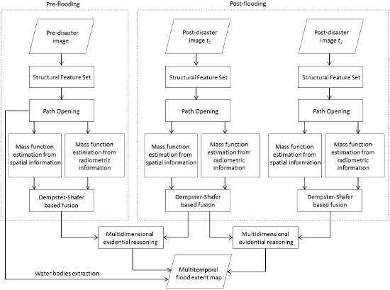
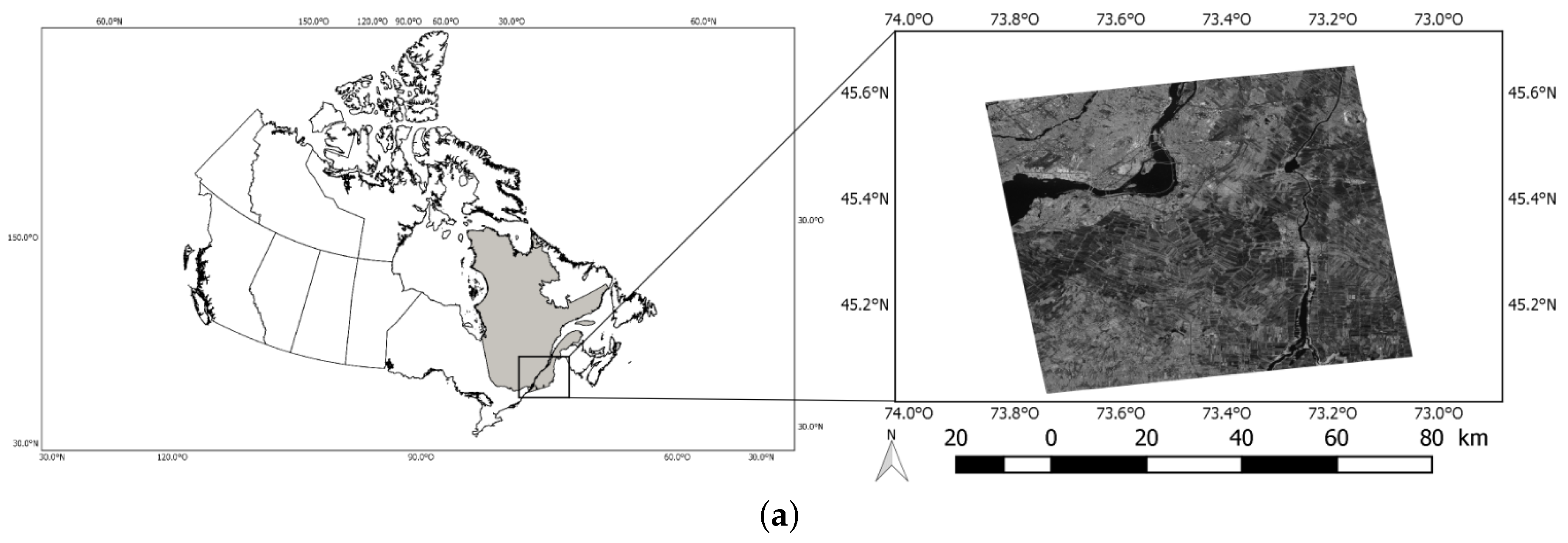
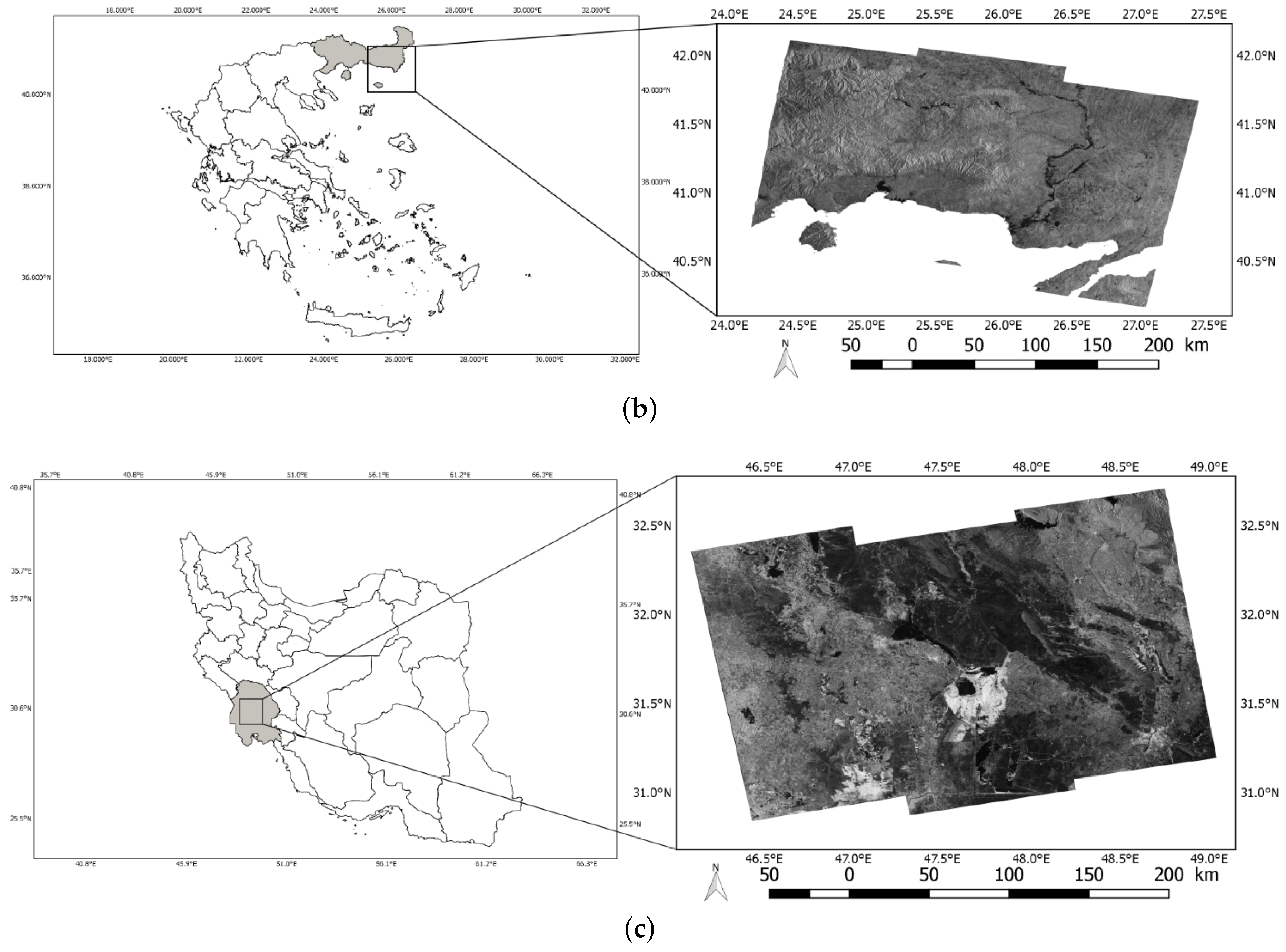
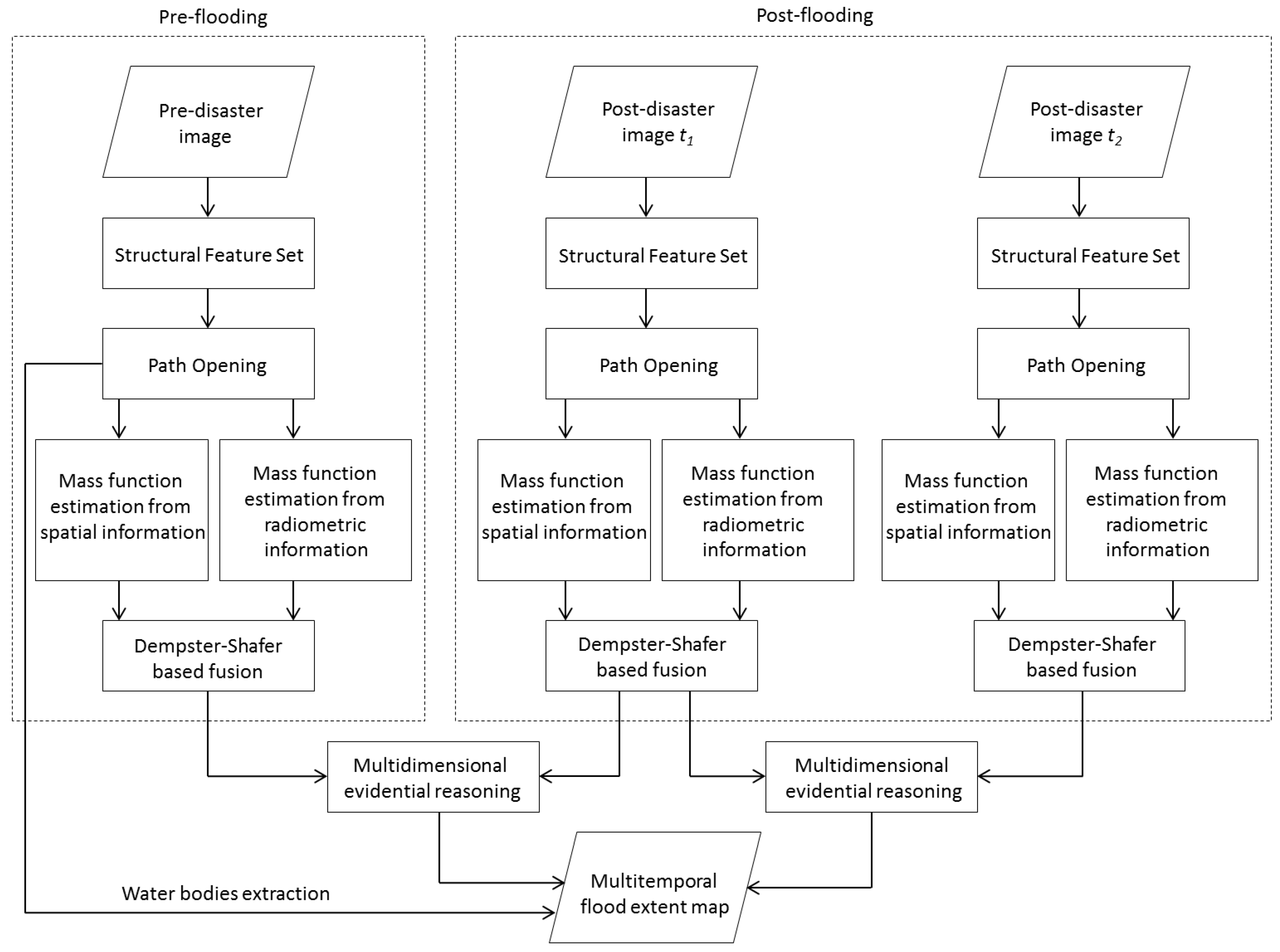
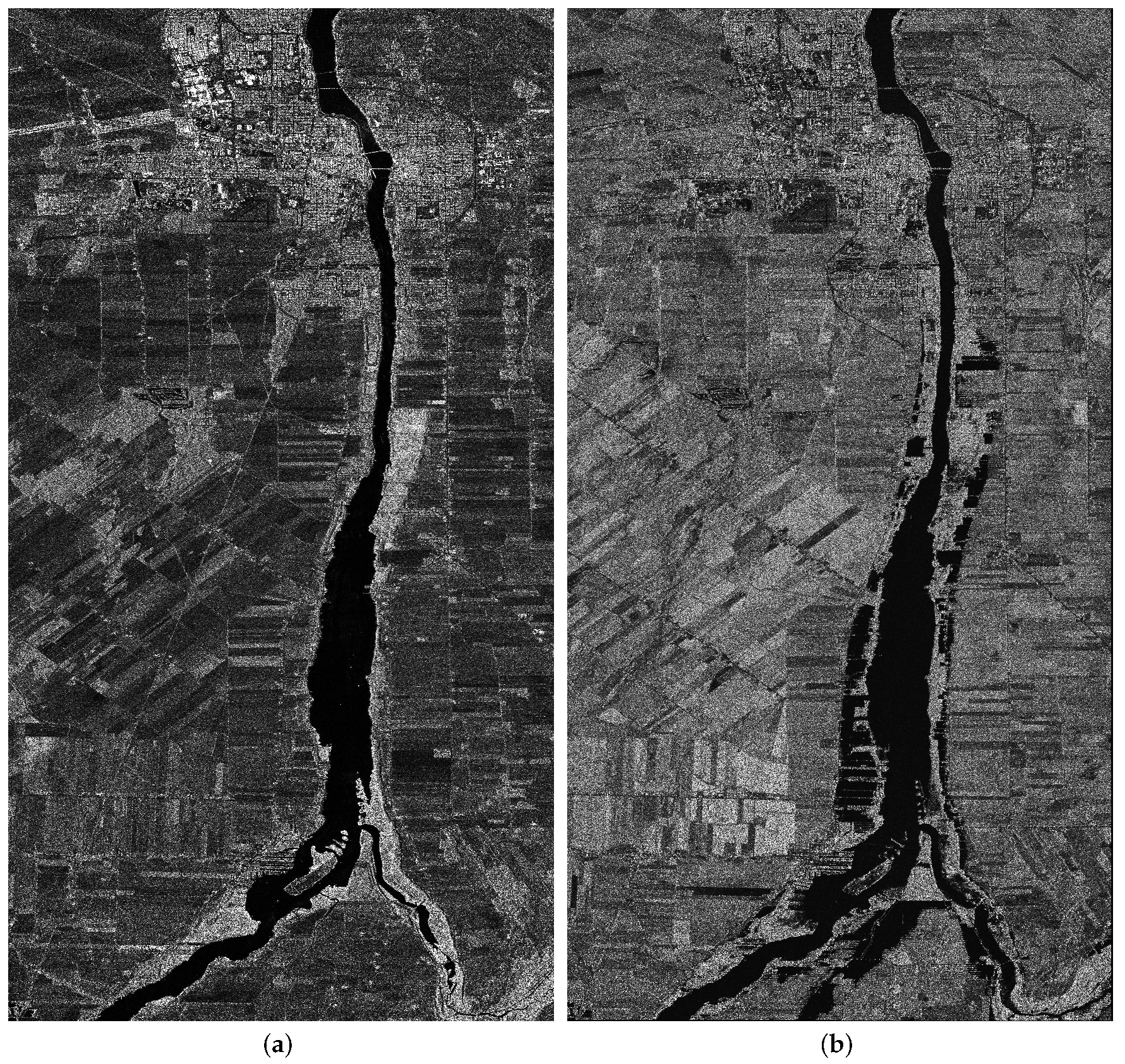
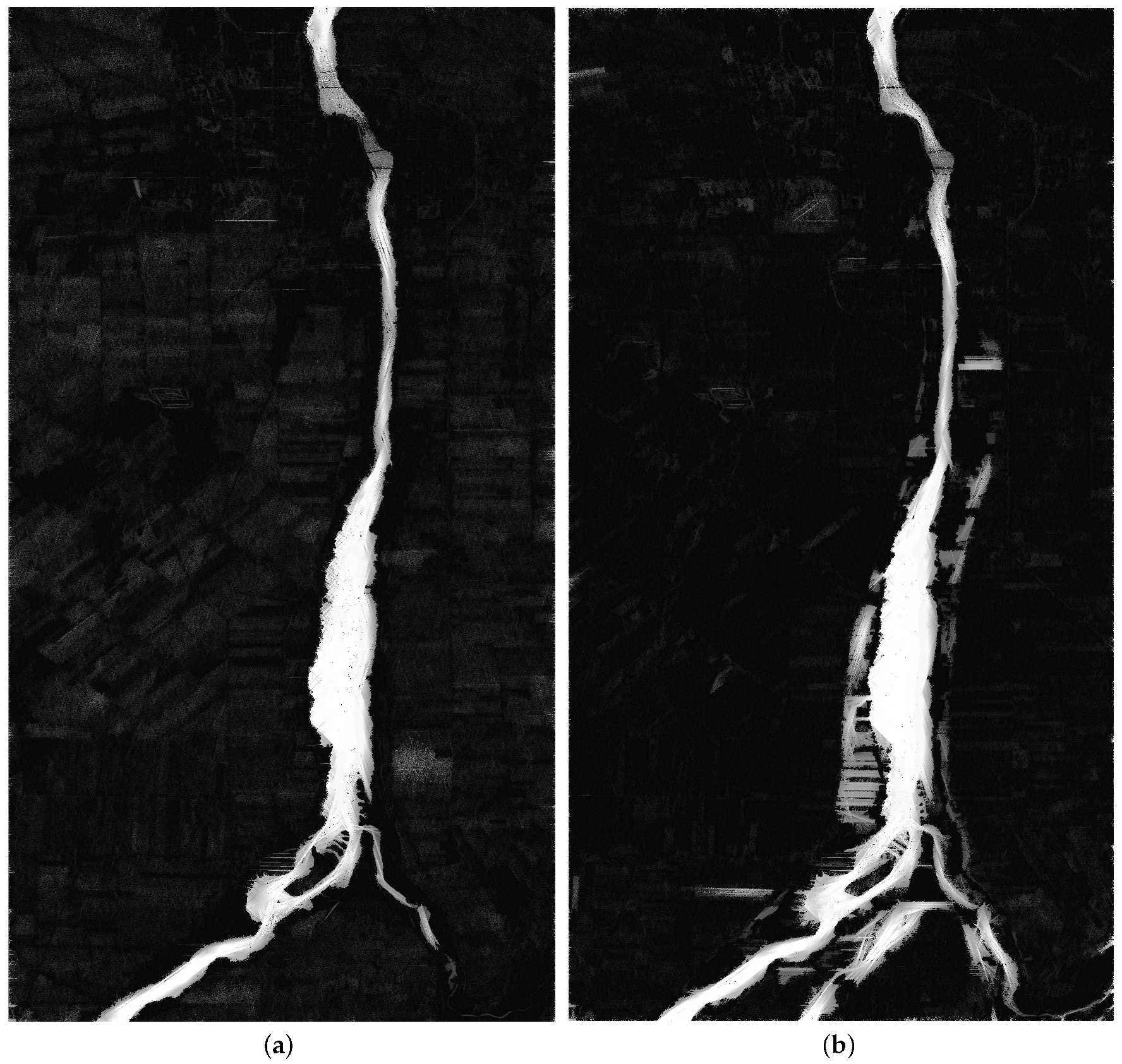
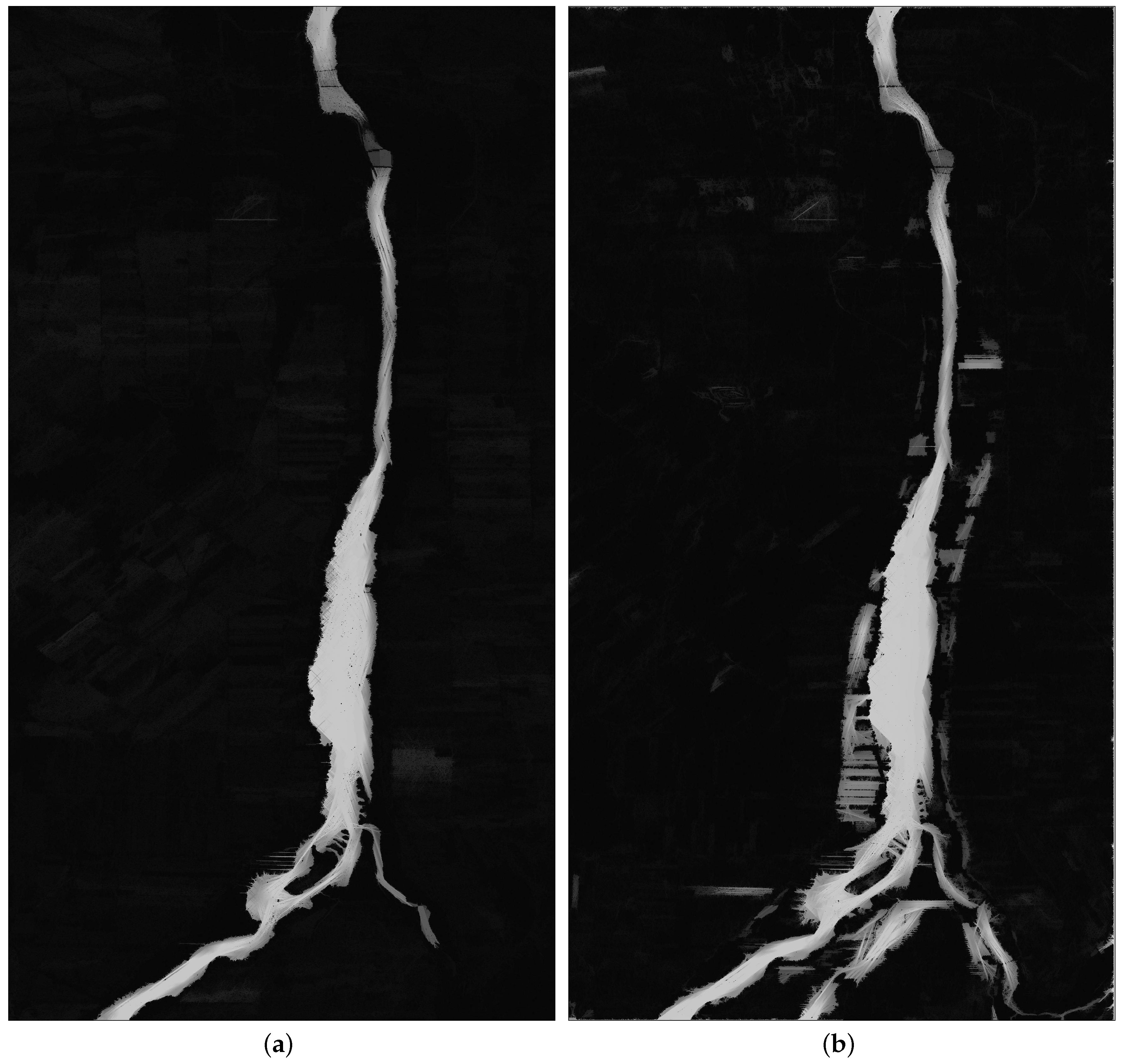
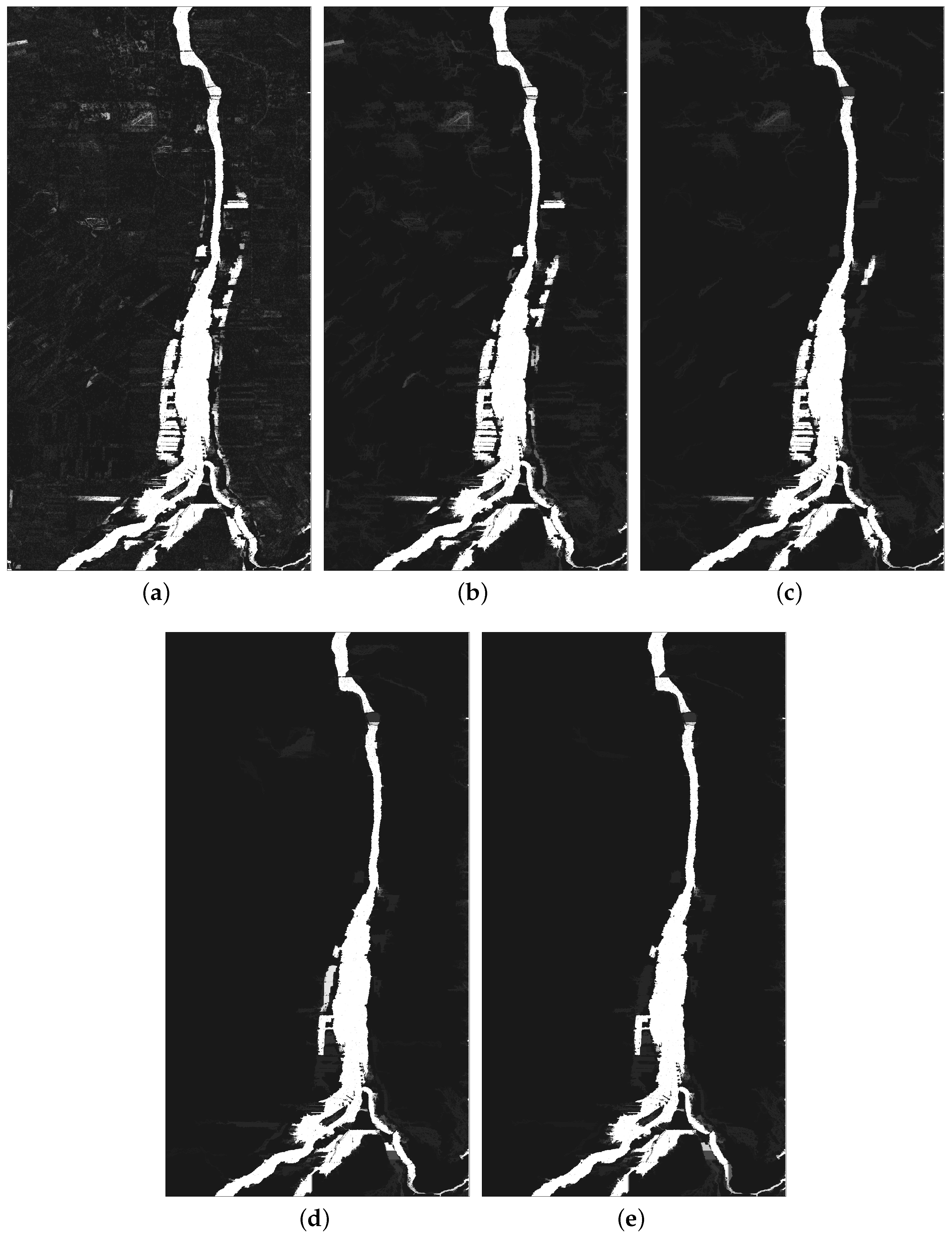
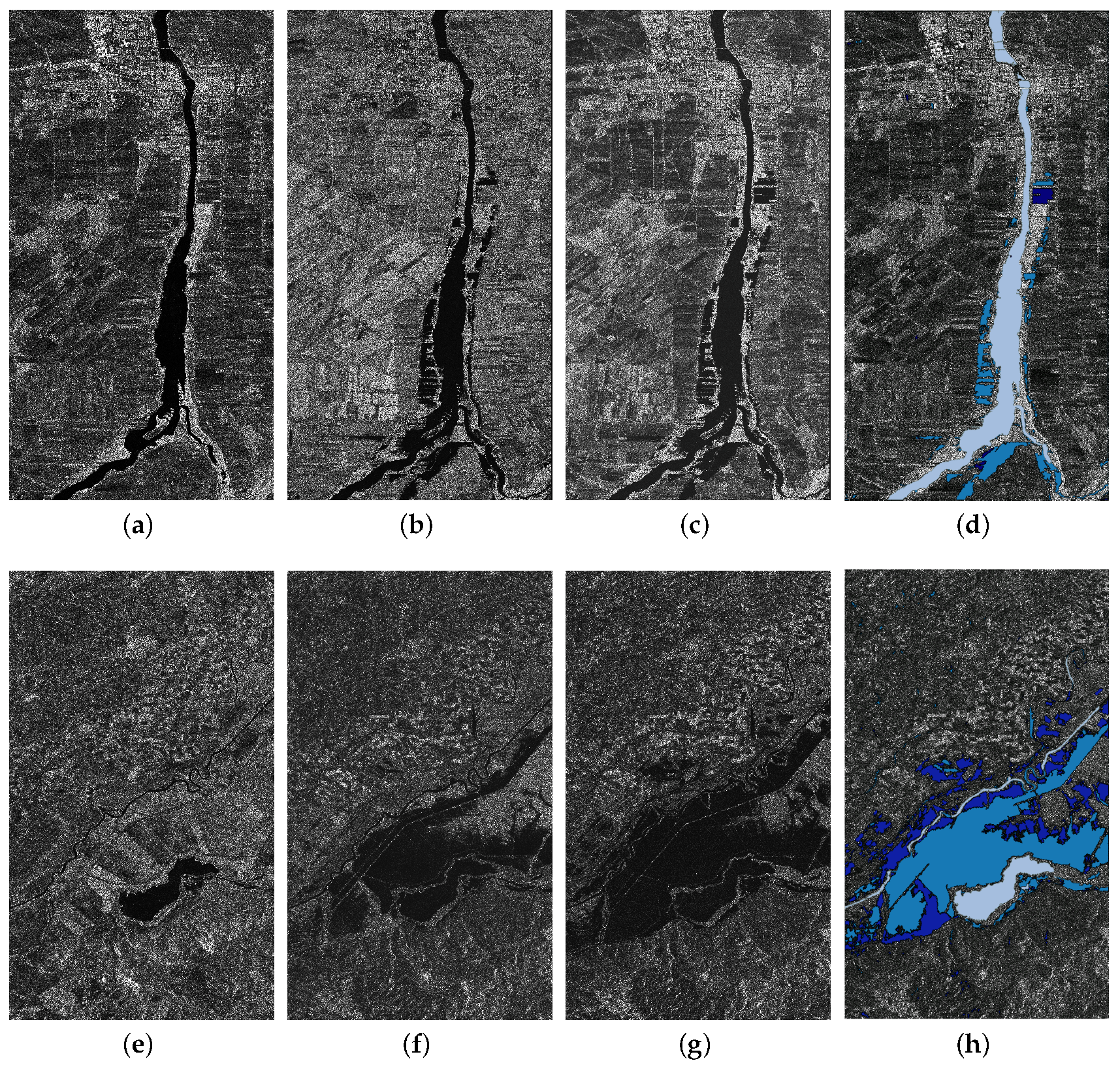
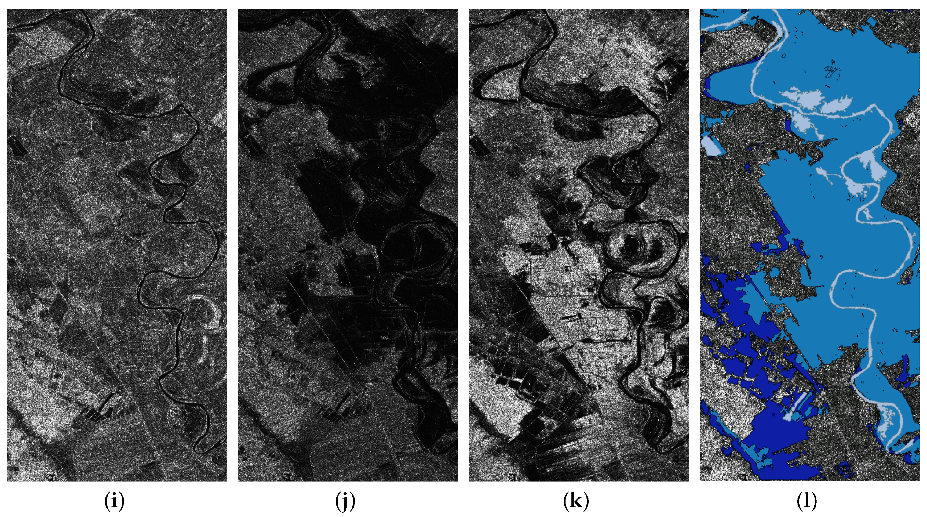
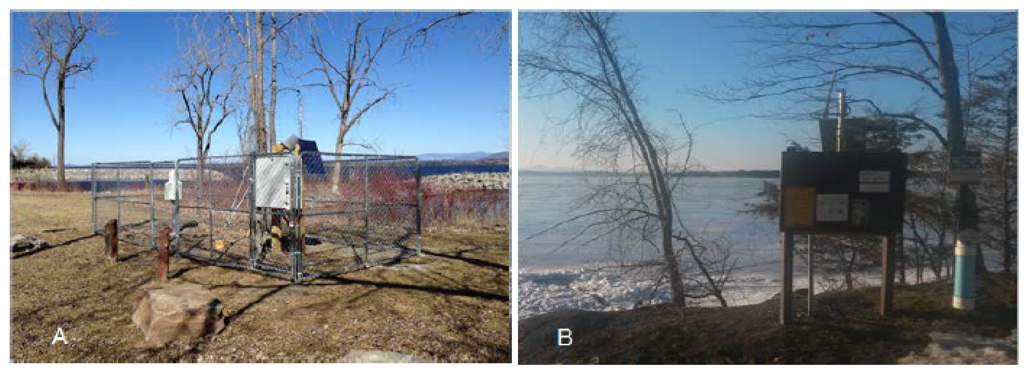
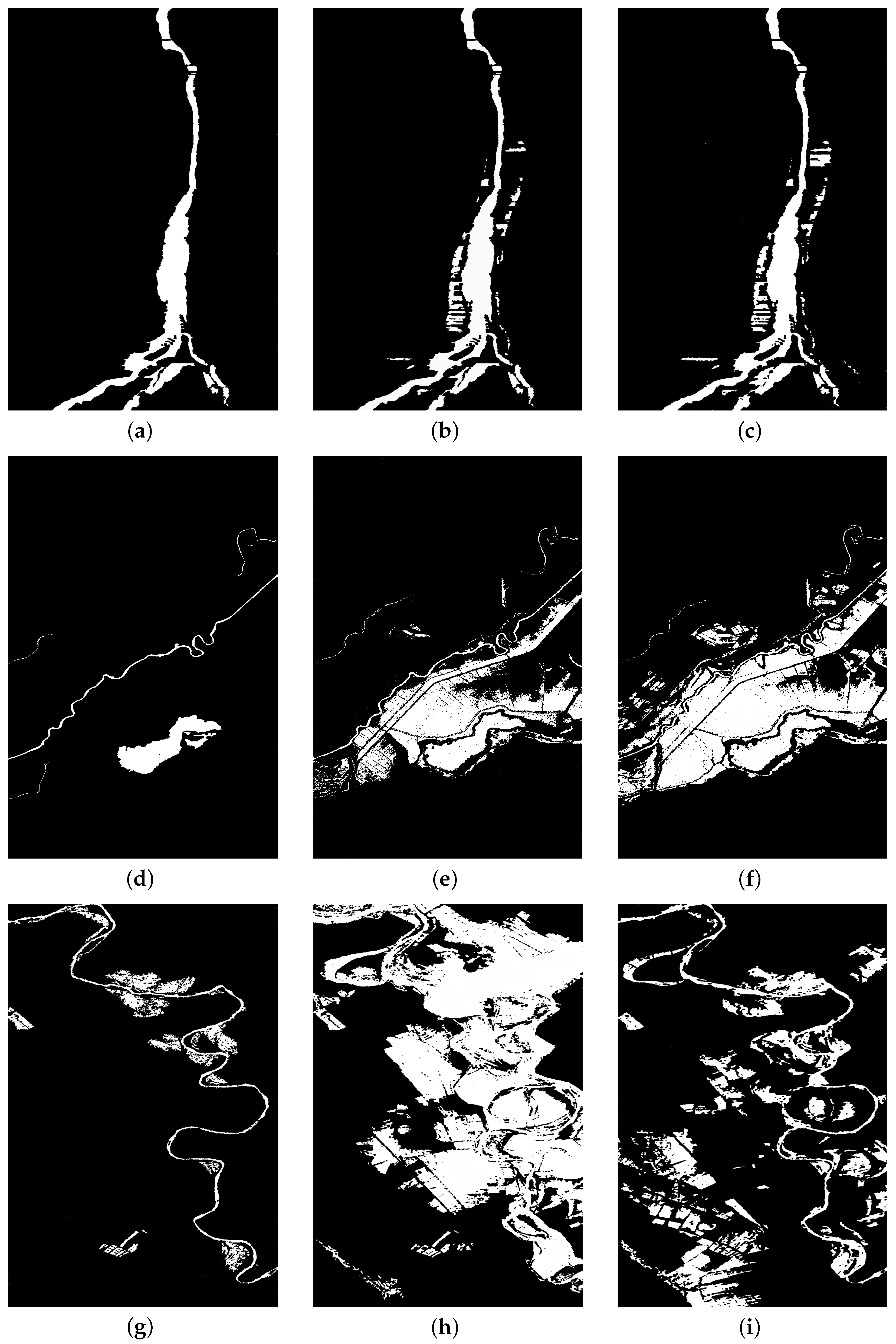
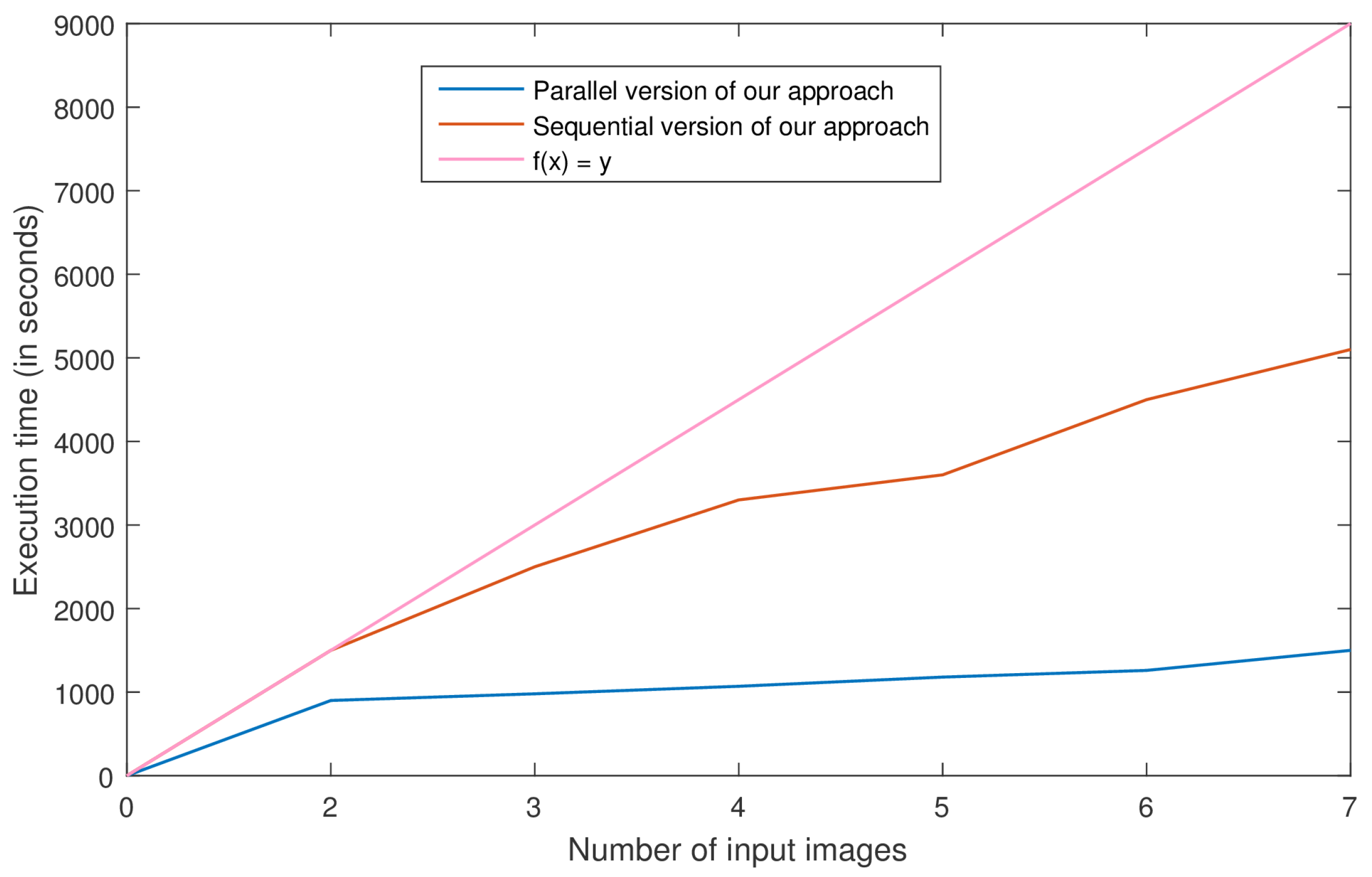
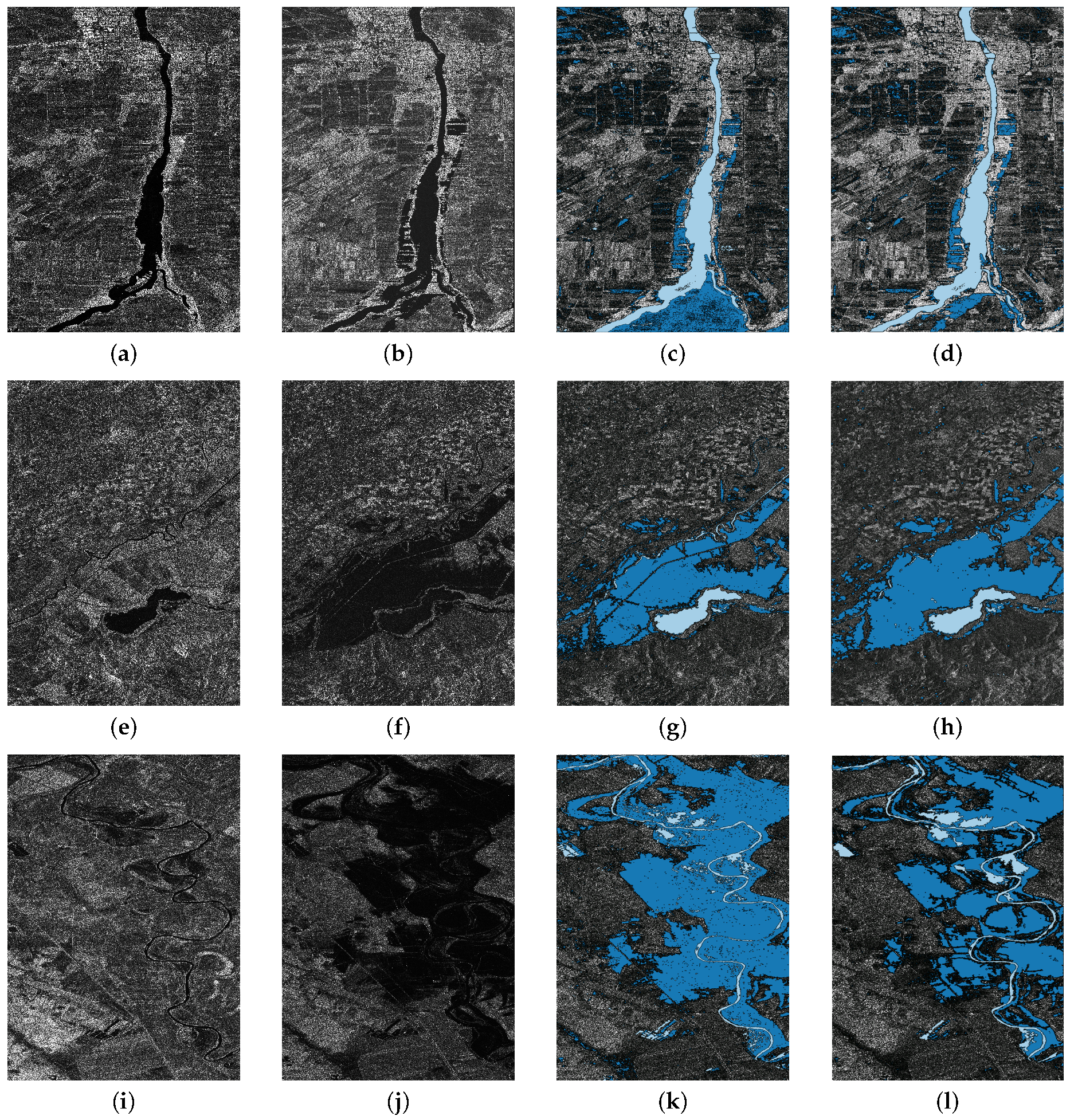
Table 1.
Summary of the SAR data properties used in this study.
| Event | Satellite | Beam | Resolution (m) | Swath Wide (km) | Incidence Angle (deg) | Number of Scenes | ||
|---|---|---|---|---|---|---|---|---|
| Near | Far | Asc. | Des. | |||||
| 1 | RADARSAT-2 | F23 | 8 | 45 | 30 | 33.4 | 4 | 1 |
| F22 | 8 | 45 | 32.4 | 35.7 | 1 | 0 | ||
| F2 | 8 | 45 | 39.3 | 42.1 | 1 | 0 | ||
| F3 | 8 | 45 | 41.4 | 44.1 | 1 | 1 | ||
| F5 | 8 | 45 | 45.2 | 47.7 | 1 | 4 | ||
| F6 | 8 | 45 | 46.9 | 49.3 | 2 | 3 | ||
| 2 | Sentinel-1 | IW | 12 | 250 | 29.1 | 46.0 | 2 | 3 |
| 3 | Sentinel-1 | IW | 12 | 250 | 29.1 | 46.0 | 4 | 1 |
| Total | 16 | 13 | ||||||
| 29 | ||||||||
Table 2.
Results obtained using our evaluation metric.
| Site 1 | Site 2 | Site 3 | |||||||
|---|---|---|---|---|---|---|---|---|---|
| Acc | Pre | Rec | Acc | Pre | Rec | Acc | Pre | Rec | |
| SFS-SD | 0.93 | 0.13 | 0.53 | 0.83 | 0.1 | 0.88 | 0.72 | 0.1 | 0.7 |
| SFS-SD + Path opening | 0.97 | 0.48 | 0.8 | 0.88 | 0.35 | 0.9 | 0.83 | 0.3 | 0.79 |
| SFS-SD + Path opening + Bayesian-based fusion [51] | 0.96 | 0.79 | 0.81 | 0.87 | 0.71 | 0.8 | 0.7 | 0.76 | 0.69 |
| SFS-SD + Path opening + Fuzzy logic-based fusion [52] | 0.98 | 0.82 | 0.85 | 0.9 | 0.73 | 0.83 | 0.73 | 0.8 | 0.72 |
| Our approach | 0.993 | 0.92 | 0.9 | 0.93 | 0.89 | 0.91 | 0.88 | 0.86 | 0.85 |
© 2018 by the authors. Licensee MDPI, Basel, Switzerland. This article is an open access article distributed under the terms and conditions of the Creative Commons Attribution (CC BY) license (http://creativecommons.org/licenses/by/4.0/).
Share and Cite
MDPI and ACS Style
Ouled Sghaier, M.; Hammami, I.; Foucher, S.; Lepage, R. Flood Extent Mapping from Time-Series SAR Images Based on Texture Analysis and Data Fusion. Remote Sens. 2018, 10, 237. https://0-doi-org.brum.beds.ac.uk/10.3390/rs10020237
AMA Style
Ouled Sghaier M, Hammami I, Foucher S, Lepage R. Flood Extent Mapping from Time-Series SAR Images Based on Texture Analysis and Data Fusion. Remote Sensing. 2018; 10(2):237. https://0-doi-org.brum.beds.ac.uk/10.3390/rs10020237
Chicago/Turabian StyleOuled Sghaier, Moslem, Imen Hammami, Samuel Foucher, and Richard Lepage. 2018. "Flood Extent Mapping from Time-Series SAR Images Based on Texture Analysis and Data Fusion" Remote Sensing 10, no. 2: 237. https://0-doi-org.brum.beds.ac.uk/10.3390/rs10020237
Note that from the first issue of 2016, this journal uses article numbers instead of page numbers. See further details here.