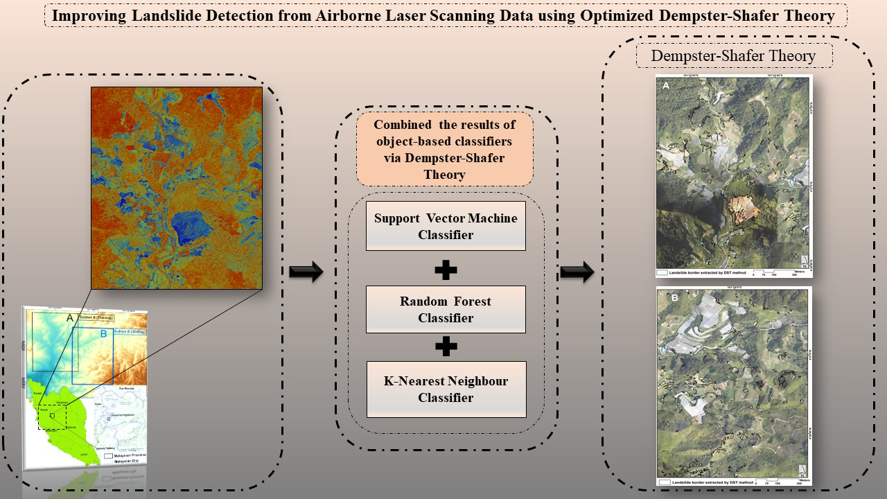
Improving Landslide Detection from Airborne Laser Scanning Data Using Optimized Dempster–Shafer


1
School of Systems, Management and Leadership, Faculty of Engineering and IT, University of Technology Sydney, CB11.06.106, 81 Broadway, Ultimo, NSW 2007, Australia
2
Department of Energy and Mineral Resources Engineering, Choongmu-gwan, Sejong University, 209 Neungdong-ro, Gwangjin-gu, Seoul 05006, Korea
*
Author to whom correspondence should be addressed.
Remote Sens. 2018, 10(7), 1029; https://0-doi-org.brum.beds.ac.uk/10.3390/rs10071029
Submission received: 28 April 2018
/
Revised: 26 June 2018
/
Accepted: 26 June 2018
/
Published: 29 June 2018
(This article belongs to the Special Issue Landslide Hazard and Risk Assessment)
Abstract
:A detailed and state-of-the-art landslide inventory map including precise landslide location is greatly required for landslide susceptibility, hazard, and risk assessments. Traditional techniques employed for landslide detection in tropical regions include field surveys, synthetic aperture radar techniques, and optical remote sensing. However, these techniques are time consuming and costly. Furthermore, complications arise for the generation of accurate landslide location maps in these regions due to dense vegetation in tropical forests. Given its ability to penetrate vegetation cover, high-resolution airborne light detection and ranging (LiDAR) is typically employed to generate accurate landslide maps. The object-based technique generally consists of many homogeneous pixels grouped together in a meaningful way through image segmentation. In this paper, in order to address the limitations of this approach, the final decision is executed using Dempster–Shafer theory (DST) rule combination based on probabilistic output from object-based support vector machine (SVM), random forest (RF), and K-nearest neighbor (KNN) classifiers. Therefore, this research proposes an efficient framework by combining three object-based classifiers using the DST method. Consequently, an existing supervised approach (i.e., fuzzy-based segmentation parameter optimizer) was adopted to optimize multiresolution segmentation parameters such as scale, shape, and compactness. Subsequently, a correlation-based feature selection (CFS) algorithm was employed to select the relevant features. Two study sites were selected to implement the method of landslide detection and evaluation of the proposed method (subset “A” for implementation and subset “B” for the transferrable). The DST method performed well in detecting landslide locations in tropical regions such as Malaysia, with potential applications in other similarly vegetated regions.
Keywords:
DST; object-based approach; landslide detection; LiDAR; GIS; remote sensing; Dempster-Shafer theory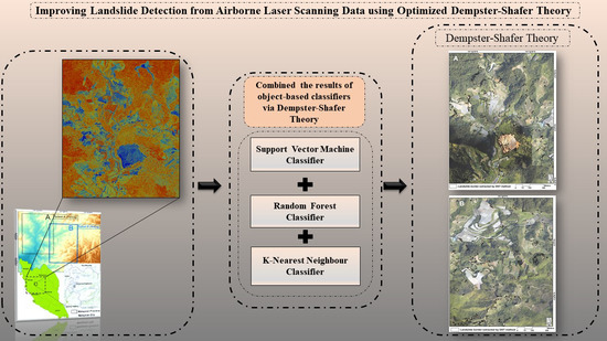
1. Introduction
Landslide inventory maps may provide baseline information about landslide types, distribution, location, and boundaries in landslide-prone areas. Information pertaining to slope and displacement measurements affecting failure may be deduced from landslide inventories [1]. Furthermore, landslide inventories could be deployed for various purposes, such as implementation of landslide susceptibility, hazard assessment, risk assessment, and landslide magnitude recording. It is a quite challenging task to map landslide inventory in tropical areas due to densely vegetative cover which obscures the underlying landforms [2]. However, most of the available traditional landslide detection methods, such as optical and aerial photographs, high spatial resolution multispectral images, synthetic aperture radar (SAR) images, very high resolution (VHR) satellite images, and moderate-resolution digital terrain models (DTM) [3,4,5,6] are not sufficiently quick and accurate enough to map landslide inventory due to rapid vegetation growth in tropical areas. Thus, a fast and accurate approach is required in landslide inventory mapping. Therefore, high-resolution light detection and ranging (LiDAR)-derived digital elevation models (DEMs) may provide highly valuable information on landslide-prone terrain shielded by densely vegetative cover [7]. High-resolution DEM may be employed to detect landforms and provide useful information about densely vegetated and rocky areas; consequently, minimal changes in topographic features may be easily detected [8,9,10]. Generally, LiDAR data could propose significant benefits, owing to their ability to penetrate dense vegetation and provide valuable information on topographic conditions [2]. These benefits make LiDAR data unique and different from other data sources, such as aerial photographs for slope failure detection under dense vegetation [4,6].
Pixel-based approaches often exhibit a “salt and pepper” appearance when very high spatial resolution images are employed [11]. However, an object-based method is widely utilized in landslide mapping to resolve the aforementioned pixel-based limitations [12]. According to Moosavi et al. [13], it is usually assumed that a pixel is very likely to belong to the same class as its neighboring pixels. In contrast to the information obtained from individual pixels, object-based image analysis offers additional geometric and contextual information that can be derived from image objects [5,12]. In an object-based approach, one of the most challenging issues is selecting the optimum combination of segmentation parameters [13]. According to Zeng et al. [14], the Dempster–Shafer theory (DST) is a precise fusion algorithm utilizing belief uncertainty intervals to present the belief of assumptions based on evidence of multiple observations. The algorithm utilizes reasoning, weight, and probability-driven evidences contained within the dataset [14]. The ability to handle incomplete data and an associated degree of uncertainty gives DST the strength to exploit data from many sensors in a processing train [15]. The reasoning-based system [16] and the empirical determination of parameters in DST make the concept generally applicable without depending on satellite imagery [15]. Furthermore, it is an economical and time-effective alternative, as it decreases the time required to select training sites [17]. From the literature, it is apparent that the DST method has previously been employed for multisensor images [18]. In the current study, the DST method was applied to fuse three object-based classified maps at the feature level. This approach (DST) has been tested in many other applications, such as fingerprint verification, forensics, ontologies, and the military [19,20,21]. Also, the model has been used in remote sensing applications such as mapping landslide susceptibility [22,23,24,25], groundwater assessment and potentials [26], and risk assessment of groundwater pollution [27]. In 2017, Mezaal et al. [28] applied the DST method for automatic detection of landslide locations using very high LiDAR-derived data and orthophoto imagery.
Landslides have the capability to display heterogeneous sizes that require information with higher spatial resolutions in order to produce complete event inventories [29]. Effective feature selection, such as texture, image band information, and geometric features, are needed to improve the quality of landslide inventory mapping. However, handling huge amount of irrelevant features can lead to overfitting [3]. Landslide identification in a particular area may be improved by selecting the most significant features [3,6,7,8,9]. According to Van Westen et al. [8], selection of the most significant features may aid in distinguishing between landslides and non-landslides. Researchers such as Stumpf and Kerle [30] have attempted to improve the efficiency of feature selection in detecting the location of landslides. Some object-based investigations have taken care of feature selection to detect landslides using LiDAR data [3,31]. Recently, Pradhan and Mezaal [2] effectively utilized a correlation-based selection method (CFS) to optimize the feature selection for detecting landslides in tropical areas.
Therefore, the present study proposes an improved approach to detect landslide locations by employing a Dempster–Shafer theory (DST) fusion technique. In this technique, three object-based classified outputs are fused together (in contrast to multisensor data) to achieve more efficient and accurate results.
2. Materials and Methods
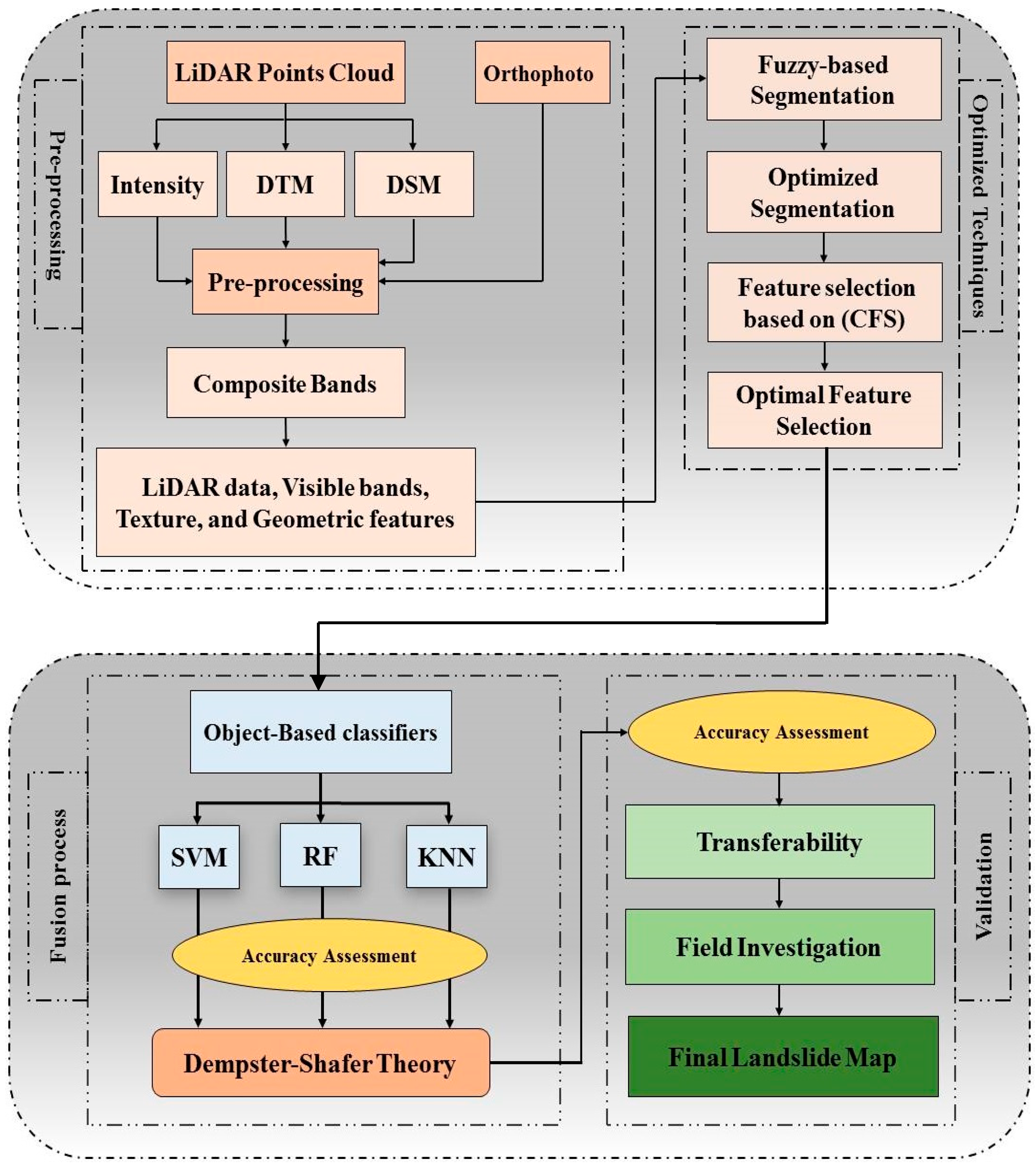
The investigation started with the preprocessing of LiDAR data and landslide inventories, an essential step typically taken before the commencement of subsequent steps to eliminate the noise and outliers from data. Subsequently, a high-resolution DEM (0.5 m) was derived from LiDAR point clouds and utilized to produce other LiDAR-derived products and landslide conditioning factors (i.e., aspect, slope, height, normalized digital surface model (nDSM), intensity, and hillshade). The LiDAR-derived products and orthophotos were combined by correcting their geometric distortions and were projected in one coordinate system. Lastly, they were prepared in GIS for feature extraction. Thereafter, a fuzzy-based segmentation parameter optimizer (FbSP optimizer), developed by Zhang et al. [32], was employed to acquire suitable parameters (i.e., shape, scale, and compactness) in differing levels of segmentation. Next, three object-based approaches—support vector machine (SVM), random forest (RF), and K-nearest neighbor (KNN) classifiers—were applied for both analysis and test areas. Subsequently, DST was employed to combine the outputs of the aforementioned classifiers in MATLAB R2015b. Model transferability was applied to another part of the study area (i.e., test site). The results were then validated and compared based on quantitative and qualitative methods (i.e., confusion matrix and precision/recall). Figure 1 illustrates a detailed flowchart of the methodology and the overall framework.
2.1. Study Area
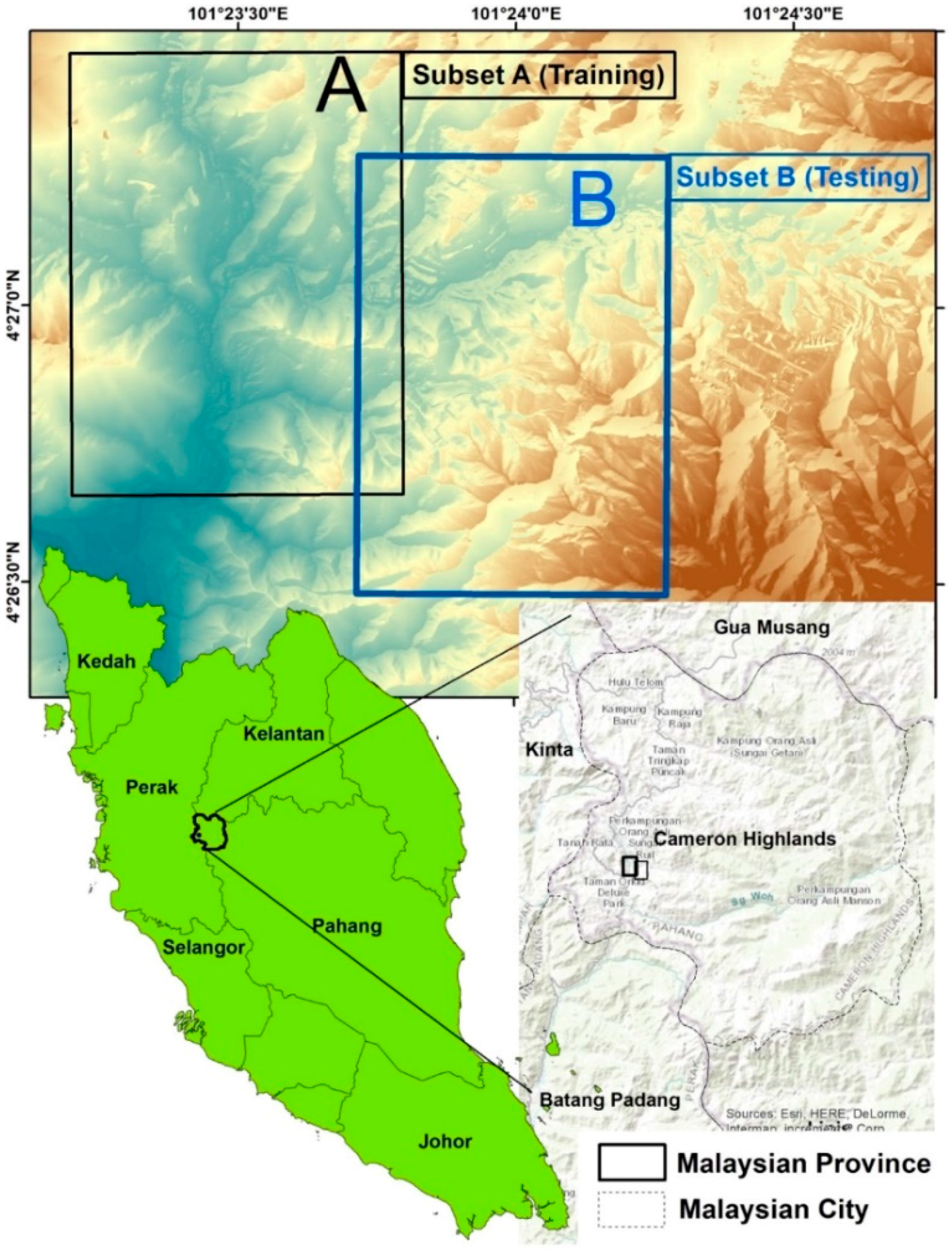
The present investigation was carried out in the tropical, densely vegetated rainforest of Cameron Highlands, Malaysia. The rationality for choosing this study area was the frequent occurrence of landslides there. Geographically, the area under consideration is located in the north of peninsular Malaysia (latitude 4°26′09″N–4°27′30″N and longitude 101°23′02″E–101°23′47″E), covering an area of 26.7 km2. The study area records an annual average rainfall of about 2660 mm and average temperatures of 24 °C and 14 °C during day and night times, respectively. A significant portion of the study area (80%) is forested landform, ranging from flat terrain (0°) to hilly area (80°).
In the present investigation, two subsets were selected to implement the proposed method, shown in Figure 2. A training area was employed to enhance the methodology for detecting the location of landslides. Similarly, a testing site was employed for testing purposes. Meticulous care was taken in selecting the test site to avoid deficiencies in the number of classes. Moreover, the training sample size was assessed using stratified random sampling method in order to enhance the accuracy of the subsets under consideration (i.e., training and test sites).
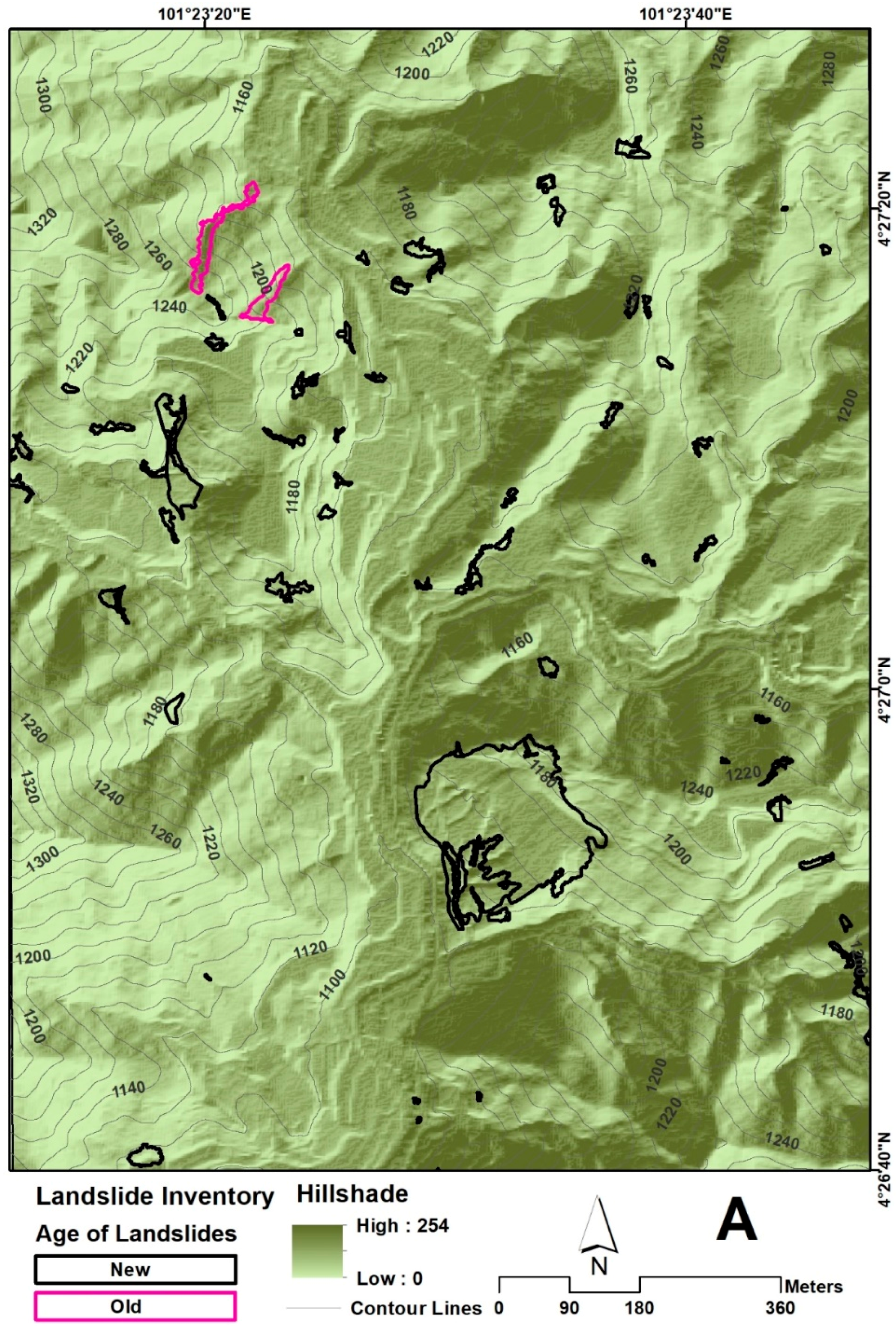
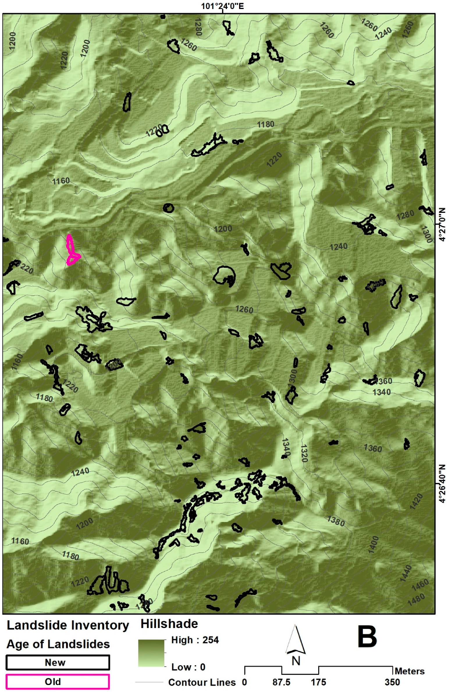
Generally speaking, landslide history is an important aspect of landslide detection. It gives an idea of its occurrences in a particular region. In this regard, landslide history was collected from many sources such as newspapers, national reports, technical papers, etc. The preliminary classification was based on age for landslide inventory mapping in accordance with visible morphologic criteria captured on aerial photographs. Landslide deposits and scars are disequilibrium landforms that evolve through morphologic stages with age [33]. Specifically, relevant information from previous investigations and landslide inventory information spanning over a decade was prepared for the whole Cameron Highlands. In an earlier paper by Pradhan and Lee [34], a database of 324 landslide incidents was prepared for 293 km2 of the Cameron Highlands to assess the number of landslides and their corresponding surface area. It was observed that the landslides are shallow rotational and a few translational types. The data was put together based on historical landslide records. In March 2011, AIRSAR data was deployed to prepare the landslide inventory map. In 2014, Samy and Marghany [35] presented the landslide history of 273 landslides of different sizes collected from the archive data of the Department of Mineral and Geosciences, Malaysia. In the same year, Murakmi et al. [36] prepared a database of historical landslide occurrences in the Malaysian Peninsula. In 2015, Shahab and Hashim [37] reported a landslide history prepared from different sources, such as field surveys, published reports, and digital aerial photographs (DAP) covering a 25-year period. Therefore, landslides can be characterized as old and new events using visual inspection and overlaying the last landslides events on the Cameron Highlands. Due to vegetation cover, landslides which have occurred between 2008 and 2010 are considered old landslides. On the other hand, new landslides are those which have occurred after 2010. New landslides less than 5-years old are apparently barren in nature and can be observed by red, green, and blue (RGB) sensors. However, the ones older than 5 years are usually covered by vegetation and thus cannot be recognized in visible bands. Figure 3 and Figure 4 show the landslide inventory map for both subsets (training and test sites), respectively.
2.2. Data Used
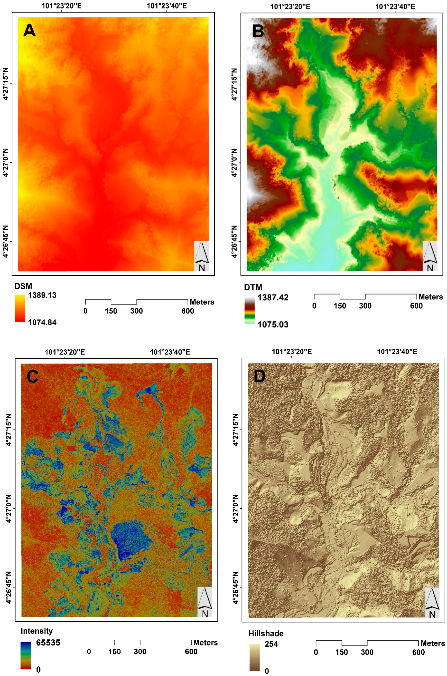
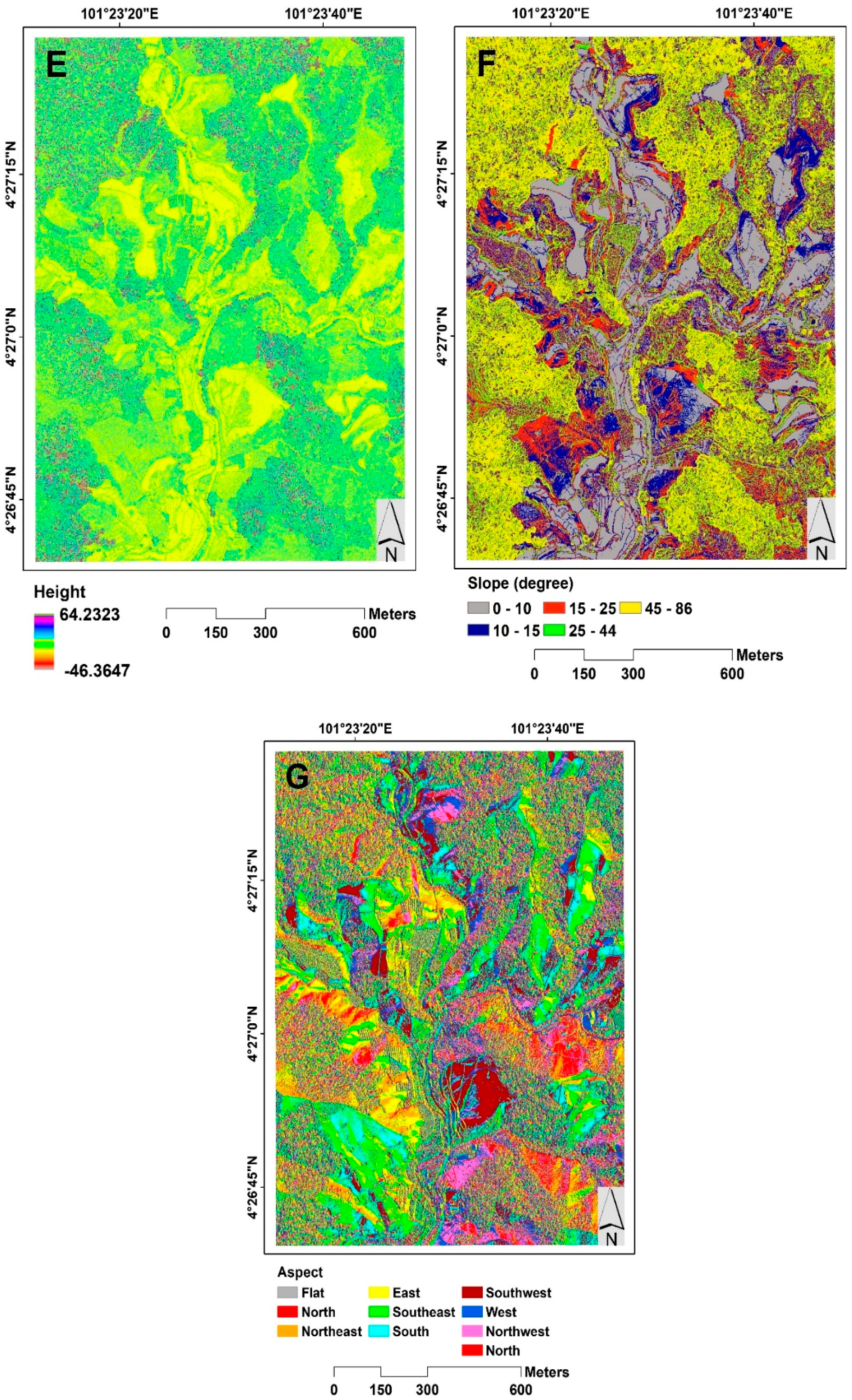
The LiDAR point cloud data was captured for the Cameron Highlands region on January 15, 2015. The land area spans 26.7 km2 of the Ringlet at an altitude of 1510 m. The point density is approximately 8 points per square meter, with a 25,000-Hz pulse rate frequency. The accuracy of the LiDAR data was restricted to conform to the root-mean-square errors of 0.15 m and 0.3 m in the vertical and horizontal axes, respectively, as standardized by the Department of Survey and Mapping Malaysia (JUPEM). A high-resolution camera (visible bands) used in the acquisition of LiDAR point cloud data in the study area was deployed to collect the orthophotos. A DSM was generated by interpolating LiDAR point clouds using inverse distance weighting method (IDW) using the ArcGIS 10.3 software (Figure 5A). A DEM of spatial resolution of 0.5 m was interpolated from the LiDAR point clouds after removing the nonground points using inverse distance weighting, with GDM2000 as the spatial reference (Figure 5B). Next, the height feature, i.e., normalized DSM (nDSM), was derived by subtracting DSM from DEM (Figure 5E). Subsequently, the LiDAR-based DEM was used to generate the derived layers in identifying the location of landslides and their features [38]. Slope is a major determinant of land stability due to its role in landslide phenomenology [39]. Hillshade refers to a map showing sufficient images of terrain movement which aid in landslide mapping [40]. The intensity image obtained from LiDAR data also play a significant role in differentiating between landslides and non-landslides [2]. Moreover, the quality of the landslide inventory map may be significantly improved by using texture features [2,6]. These data provide extensive information on landslide detection [28]. The accuracy and ability of DEM to represent the surface are affected by terrain morphology, sampling density, and the interpolation algorithm [41]. In the present study, various LiDAR-derived data were employed as follows: DEM, DSM, intensity, height (nDSM), slope, and aspect (shown in Figure 5). Additionally, orthophoto images (i.e., visible bands) and texture features were used to detect the landslides.
2.3. Multiresolution Segmentation Algorithm
A multiresolution segmentation (MRS) is a bottom-up approach used in a segmentation algorithm and is based on the pairwise region-merging technique [12]. In algorithms, image pixels that possess homogeneous spectral and textural characteristics are usually grouped [42]. The smaller objects are substituted in the larger ones based on certain criteria obtainable from three parameters: color, scale, and shape (i.e., smoothness and compactness). The aforementioned three parameters may be determined in this algorithm using the traditional trial-and-error method; however, this is a time-consuming and laborious task [4]. Hence, many semiautomatic and automatic approaches have attempted to optimize parameter segmentation [43,44,45]. Optimization techniques consider only the scale, without taking into consideration the combination of the parameters [4]. A few powerful optimization techniques currently exist, such as the Taguchi optimization method [4] and the fuzzy-based segmentation parameter optimizer (FbSP optimizer) [32]. These techniques represent advanced methods employed for automatic combination of segmentation parameters (i.e., scale, shape, and compactness). However, differentiating among image objects at various scales is still a challenge and not all feature selection methods are fully utilized in a particular segmentation scale. Thus, it is suggested that an automatic method should be directly implemented.
2.4. Calculation of the Relevant Feature Selection
Classification schemes implemented on segments are more significant than single pixels in an object-based approach. This occurs by incorporating a multitude of additional information such as the texture, shape, and context associated with image objects [46]. However, both objective and subjective methods may be used to select important object features in object-based classification. The subjective methods depend on user knowledge and past experience, while the employment of feature selection algorithms is relatively objective [47].
According to Stumpf and Kerle [30], several remote sensing applications are able to measure rotation invariance. However, they cannot capture directional patterns in the grey-value distribution. Landslide-affected areas regularly appear in a downslope direction with texture patterns. Stumpf and Kerle [30] reported that patterns are potential features for detecting and differentiating landslide surfaces and texture patterns oriented at the strike of the slope [30]. Gray-level co-occurrence matrix (GLCM) texture features can be calculated with airborne laser scanning data by using eCognition software and the measured texture co-occurrence can be calculated for individual landslide objects in the software. This result comprises Dissimilarity, Contrast, Homogeneity, and Standard Deviation co-occurrence texture measured based on all bands.
In the present study, a correlation-based feature selection algorithm (CFS) was used to select the most important features in detecting the landslide locations. The best search was utilized for determining the feature space, and the five consecutive, fully expanded, nonimproving subsets were set to a stopping criterion in order to avoid searching the entire feature subset space. In this study, the Weka 3.8 package was used to implement this feature selection algorithm. Furthermore, three employed object features resulted in 82 total features—Mean and StdDev LiDAR data, Mean and StdDev visible band, and texture (see Table 1). Mean and StdDev data were extracted from airborne laser scanning data with the use of eCognition software.
The correlation coefficient between Mean Intensity and GLCM Dissimilarity, GLCM Angular second moment, had a positive and moderate relationship at (p < 0.01), and it had a negative moderate relationship at (p < 0.01) with StdDev Blue as indicated in Table 2. The relationship between GLCM Homogeneity and GLCM Contrast and GLCM Dissimilarity were negatively correlated at (p < 0.01). However, there was positive significant relationship at (p < 0.01) with GLCM Angular second moment and StdDev Blue. The Mean Slope had a positive significant relationship at (p < 0.01) with Mean DTM and StdDev Blue, however it had a negative significant relationship at (p < 0.05) with StdDe DTM. The Mean Red showed a strong relationship at (p < 0.01) with GLCM Contrast and GLCM Dissimilarity, and it showed a negative relationship at (p < 0.05) with StdDe DTM. The correlation coefficient between Mean DTM and StdDe DTM was negatively significant at (p < 0.05). GLCM Contrast had a strong significant relationship at (p < 0.01) with GLCM Dissimilarity. The relationship between GLCM Dissimilarity and StdDev Blue was negatively significant at (p < 0.05).
2.5. Support Vector Machine (SVM)
The dataset was categorized into groups using a supervised nonparametric statistical learning technique consistent with training examples. SVMs are gaining huge popularity in various applications of remote sensing, especially in landslide mapping [13,29,48,49,50], due to their capability in handling small training datasets and unknown statistical distribution data obtained in the field [51]. Huang et al. [52] observed that SVMs containing fewer training dataset yielded more stable results compared to those of decision tree, maximum belief, and artificial neural network classifiers with large training datasets. SVMs are regarded as binary classifiers designed to determine the boundary of the decision region that separates the dataset features or characteristics into two regions in the feature space. In SVM, boundary optimal hyperplanes exhibiting maximum safety margins are chosen closest to the training features. These are called support vectors, which take full advantage of the margin between the classes [29]. Kernel functions have been used in the linearization of the decision boundary and were achieved by using the maps of the training data in the higher-dimensional space that have the capacity to linearly separate two classes of hyperplanes [52]. A nonlinear transformation of covariates was also conducted, transferring into high-dimensional feature space [53].
In the present study, SVM e1071 package [54] for the R statistical computing software was implemented [55]. It was observed that hyperparameters determined the performance of the SVM classifier. Therefore, the selection of these parameters was optimized and their sensitivity analyzed. Three parameters were assessed in the case of SVM, namely, the penalty parameter (C), kernel function, and gamma parameter (ɤ). The most accurate prediction was attained in the radial basis function (RBF), using gamma parameter (ɤ) 0.9 and penalty parameter of 300. This was carried out rapidly by visual inspection of the match between results and reference data. Seventy percent (70%) of the inventory map, along with all the features, were selected as training sets to train the RF model.
2.6. Random Forest (RF)
The RF classifier method has been implemented for detecting landslides using many types of remote sensing data [3,30,56,57,58,59]. The algorithm builds upon multiple decision trees that depend on randomly selected subsets of the training dataset. The RF makes use of the high variance among individual trees in a classification problem by assigning the respective classes based on majority votes. The merit of this approach lies in its performance on complex datasets, with fewer attempts for fine-tuning [30]. RF is defined as a random subset of the original set of features, whereas a classification and regression tree considers all variables in each node. Users can estimate the number of variables per node by using the square root of the total variable number. Various mechanisms, such as sampling and usage of random variables, in each node may produce entirely different uncorrelated trees. Moreover, large numbers of trees are absolutely required to obtain variability in the training data and attain accurate classification. A total vote of all the trees in the forest is used to determine a feature and the class will then be assigned on the basis of the majority vote.
RF package [54], an open-source statistical language R, was used in this research. The parameters used in the analysis were the number of variables in the random subset at each node and the number of trees in the forest. The number (500) of trees was chosen, which is a typical value for the RF classifier [30]. A single randomly split variable was employed to grow the trees. The inventory map (70%) together with other features and feature subsets were chosen as training sets to train the RF model. The remaining 30% of the inventory was used to evaluate the accuracy of the classification. The mean and standard deviation (stdev) values of the classification accuracies were then obtained from 50 random runs.
2.7. K-Nearest Neighbour (KNN)
KNN is a powerful tool utilized in many object-based workflows due to its flexibility and simplicity [60,61]. It is used most often for classification in object-based software frameworks, i.e., eCognition (Trimble Geospatial, Munich, Germany). In comparison to model-based learning, KNN allocates the object to the class based on proximity or neighborhood in the feature space, rather than learning from a model [62]. The closest K neighbors are obtained from the training set and then used to vote for the final predicted new object. K is usually a tunable parameter, typically assuming a small and positive integer value [5]. In this study, an optimal K parameter was used based on cross-validation and bootstrap samples which were used to search for the best K value, where K ranges from 1 to 10 in steps of 1 and the best value is applied to the KNN algorithm implemented in the R package “class”. The inventory map (70%) together with all the features were selected as training sets to train the KNN model.
2.8. Dempster–Shafer Theory
The DST is built on a frame of discernment, formally defined as the set of mutually exclusive and collectively exhaustive hypotheses, represented by Θ [62,63]. By defining two functions (Plausibility and Belief ), this theory seeks to model imprecision and uncertainty. The two functions are essentially derived from a mass function , with the latter function being applicable to every element of in lieu of exclusively to elements of θ. Thus, a rich and flexible modeling behavior is achieved which may potentially address numerous remote sensing applications. Thus, a mass function allocates belief for each proposition, shown in the following equation:
where is the empty set. Two common evidential measures within the mass function are belief and plausibility , both defined in equations:
where for every , is a measure of the total amount of beliefs committed exactly to every subset of by . signifies the degree to which the evidence remains plausible. These two functions, which are regarded as the lower and upper probabilities, respectively, contain following properties:
The rule of combination in the proposed DST builds on the mathematical theory substantiating the combination of the mass functions obtained from sources of information given in Equations (6) and (7):
where denotes the degree of conflict given in Equation (8):
Various methods exist for taking a final decision using the DST decision technique as found in the literature: the maximum mass, plausibility, or belief [28]. From the probabilistic SVM, RF, and KNN classifiers, the posterior probabilities are converted in the form of mass function . These, in turn, are then combined using the DST method. The combination output may be considered a belief function, which defines a posterior probability measure for each thematic.
2.9. Fusion of Three Object-Based Classifiers via Dempster–Shafer Theory (DST)
The fusion level analysis (FLA) method groups different classified features together and fuses them into a new class based on the belief confusion matrix [14]. In the present study, the DST algorithm was employed to perform the feature-based data fusion. This method comprises well-defined combination rules that are capable of combining several belief functions in the same frame. The theory is built on the formulated basis of harmonizing the information from many sources [64]. The evidence is then integrated in a reliable approach to complete the evaluation of the entire body of evidence. DST may serve both uncertainty and imprecision from belief and plausibility functions, while also possessing the ability to compute compound hypotheses [65].
Consequently, the results of three object-based approaches (i.e., SVM, KNN, and RF) were combined by fusing the DST with LiDAR data. The method employed the fused class label contained within each pixel with the maximal belief function. The produced fused pixels were set as an unclassified value in the case of multiple class labels [64]. For all classified landslide and non-landslide (frame of discernment), the belief functions were estimated using a precision function, which processes the confidence of a classifier probability. DST considers the majority of classified labels and then assigns that label to the segment. The belief masses for labelled features resulting from the classifiers were calculated using a confusion matrix, which is a text file that fuses the most probable feature label. Fundamentally, belief measurements are divided into four types, namely, precision, accuracy, Kappa, and recall. Due to its high performance in previous works, the precision belief function was selected in the present study to label the belief classes from standalone classifiers.
3. Results and Discussion
3.1. Optimization of Segmentation Parameters
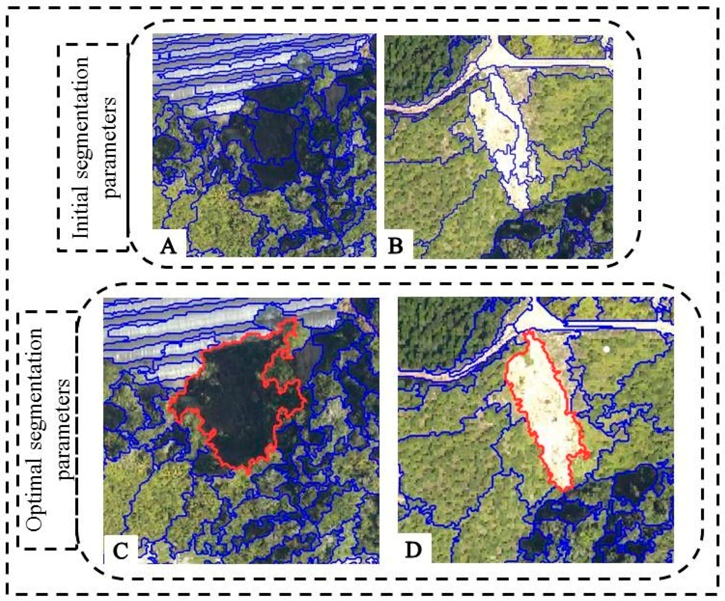
Various parameters were optimized with the FbSP optimizer, namely, the scale, shape, and compactness of the multiresolution segmentation (MRS) algorithm. This FbSP optimizer has the capability to delineate the boundaries of landslides and non-landslides, such as bare soil, vegetation, and cut slope, respectively. In this study, the values 50, 0.1, and 0.1 were used in the analysis area as the initial segmentation parameters trained in the FbSP optimizer for scale, shape, and compactness, respectively. After three iterations, the optimum values achieved in the optimizer were 75.52, 0.4, and 0.5, standing for scale, shape, and compactness, respectively (shown in Table 3). The initial and optimal segmentation processes are further illustrated in Figure 6.
Table 3 illustrates the results of segmentation parameters obtained using the FbSP optimizer. Furthermore, the segmentation of each landslide class is also highlighted. The use of the optimal segmentation parameters yielded accurate results based on the image objects produced in most classes, the results of which are depicted in Figure 6. For accurate detection of landslides, identifying and defining the parameters are extremely crucial. However, the accuracy of the result may affect the final classification map due to a certain degree of under-segmentation in some landslide locations. In case over-segmentation or under-segmentation issues arise, it becomes difficult to use the contextual and spatial features in feature identification, mainly due to the improper definition of target features. Therefore, misclassifications of the spatial and contextual features may occur with other similar features. In order to achieve result-oriented classification, it is necessary to eliminate these errors in segmentation by employing robust approaches. Therefore, combination methods could be viable alternatives to improve the accuracy of landslide classification.
3.2. Feature Subset Selection
In an attempt to obtain the optimum algorithm, CFS was used to select the most relevant feature in order to detect landslide locations. The feature input, used in the experiment, consisted of 82 LiDAR data (height, slope, and intensity), texture features (GLCM homogeneity and GLCM StdDev), and the visible band. These features were deduced using the eCognition software (see Table 4). High classification accuracy was obtained when 10 of the features indicated that visible bands, LiDAR-derived data, and textural features were applied. The values of these features contributed to separate landslides from other land cover classes such as manmade, bare land, and vegetation. It can be attributed to the landslide characteristics in the area under consideration. This illustrates the fact that visible bands, LiDAR-derived data, and textural features are effective in revealing landslide locations. Table 4 presents the most significant features selected using the CFS algorithm, showing highly important features such as Mean Intensity, GLCM Homogeneity, Mean Slope, and GLCM Angular Second Moment. Mean Red and Texture features are also significant for improving the classification accuracy. The results of the feature selection demonstrated the importance of relevant features in improving the accuracy of classification. The results of the relevant features revealed that the best combination was achieved by CFS, which improved the detection between landslide class and other land cover classes in both areas (training area and test area). Generally, selection of the most relevant feature can decrease computation time, avoid the subjective requirement of expert knowledge, and improve the classifier process.
3.3. Results of Object-Based SVM, RF, and KNN Classifiers in Training Area
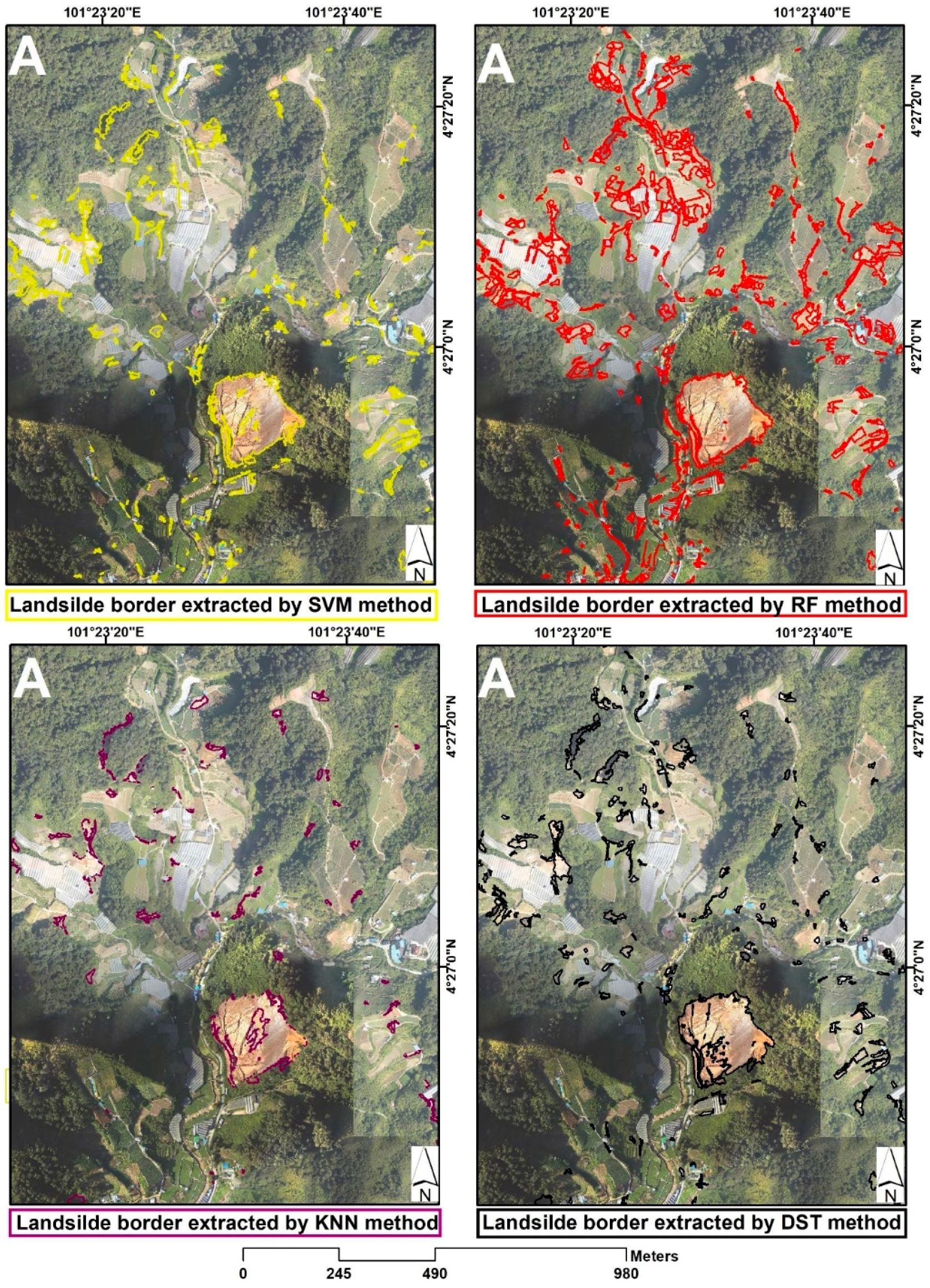
Figure 7 shows the results of RF, SVM, and KNN, which are the three object-based classifiers used in the present study. The results indicate that landslides and non-landslides were accurately classified. The results further indicate that the SVM performed excellently by creating an accurate landslide inventory map with only limited undetected landslides. Furthermore, visual assessment was found to be more reliable in SVM than in KNN and RF. Most of the landslides in the study area were identified with the aid of SVM rather than RF and KNN. The performance recorded in the SVM is a result of the two optimization techniques used to optimize the parameters of segmentation and the most relevant features selected in the classification process. Furthermore, the improvement recorded could be attributed to the parameters used in the classifiers that resulted in the classification quality. It is highly imperative to take the required measures in order to avoid landslide separation from other land cover classes, such as manmade and bare soil. This is due to the fact that the morphology features of the landslide are quite different from other types of land cover classes. For instance, the slope, shape, and other features such as depth, width, dip direction, and length of surface terrain could change after the occurrence of a landslide. Optimized landslide segments can be exploited in analysis to select the significant features. According to Van Westen et al. [8] and Mezaal et al. [64], selecting relevant features is highly imperative in distinguishing between landslides and non-landslides. Improved classification accuracy has been observed when the segments are well-fitted into landslide shapes [66,67,68]. After optimization of the feature selection in this study, it was observed that Intensity, GLCM Homogeneity, and Slope features are very significant to detect landslide locations. Hence, those features contribute to the object-based classifiers (i.e., SVM, RF, and KNN) as ancillary data in order to improve the classification results and compare with the standalone LiDAR RGB-orthophoto image. Basically, the nature of various non-landslides (e.g., cut slope and bare soil) is different in term of shape, slope, size, and texture from landslide classes. Thus, the value of the relevant features such as Intensity, GLCM Homogeneity, and Slope help to improve the classification accuracy for proper separation of the landslide classes from the bare soil or manmade classes. The OBIA classifiers were trained using the landslide inventory. Overall, all the training samples exhibited Slope values much higher than the bare soil (above 25 degrees) and the GLCM Homogeneity values are less than the manmade areas such as bright roofs (less than 0.06). Additionally, the Mean Intensity feature contributes greatly in identifying the old landslides from those that have been covered by vegetation canopy after some years. Considering the fact that all forest areas reflect similar intensity pulses, the covered old landslides under forest have higher intensity values in comparison with the surrounding areas [69]. Since a historical inventory was used to train the applied OBIA classifiers, it was observed that the Intensity value above 30,000 in forest areas reflects the old landslide location where it cannot be seen by RGB-visible bands of the orthophoto image. Then, all three classifiers expanded the trained examples to the rest of images using their own algorithms to detect the recent or old landslides out of similar non-landslide objects with different accuracy. Thus, by employing the most appropriate features derived from high-resolution LiDAR data and the texture feature could aid in distinguishing between landslides and non-landslides. However, it was observed that there exist misclassifications in identifying landslide and non-landslide classes, such as the aforementioned manmade and bare soil with other classifiers, which may affect further analysis. This would cause over-segmentation in some objects, where the structural and spatial features of landslide areas are not discriminated. In addition, this confusion is due to the degree of similarity of spatial characteristics among the aforementioned classes.
The DST method was used in the present work to combine the results of each classifier, landslide class, and belief functions. These were projected using a precision algorithm that measures the confidence of probable classifier on the bases of the resulting feature labels. The belief’s masses for feature labels, obtained from each classifier, were computed using a confusion matrix, a text file used to fuse the most probable feature label. The feature fusion of classifiers produced a single and precise landslide inventory map which combines the extracted information from the inputs’ object-based classifications and the results of the DST method, as shown in Figure 5. The validated results and maps developed substantiates the notion that the proposed method is reliable for the recognition and mapping of landslide locations.
3.4. Transferability to Test Site
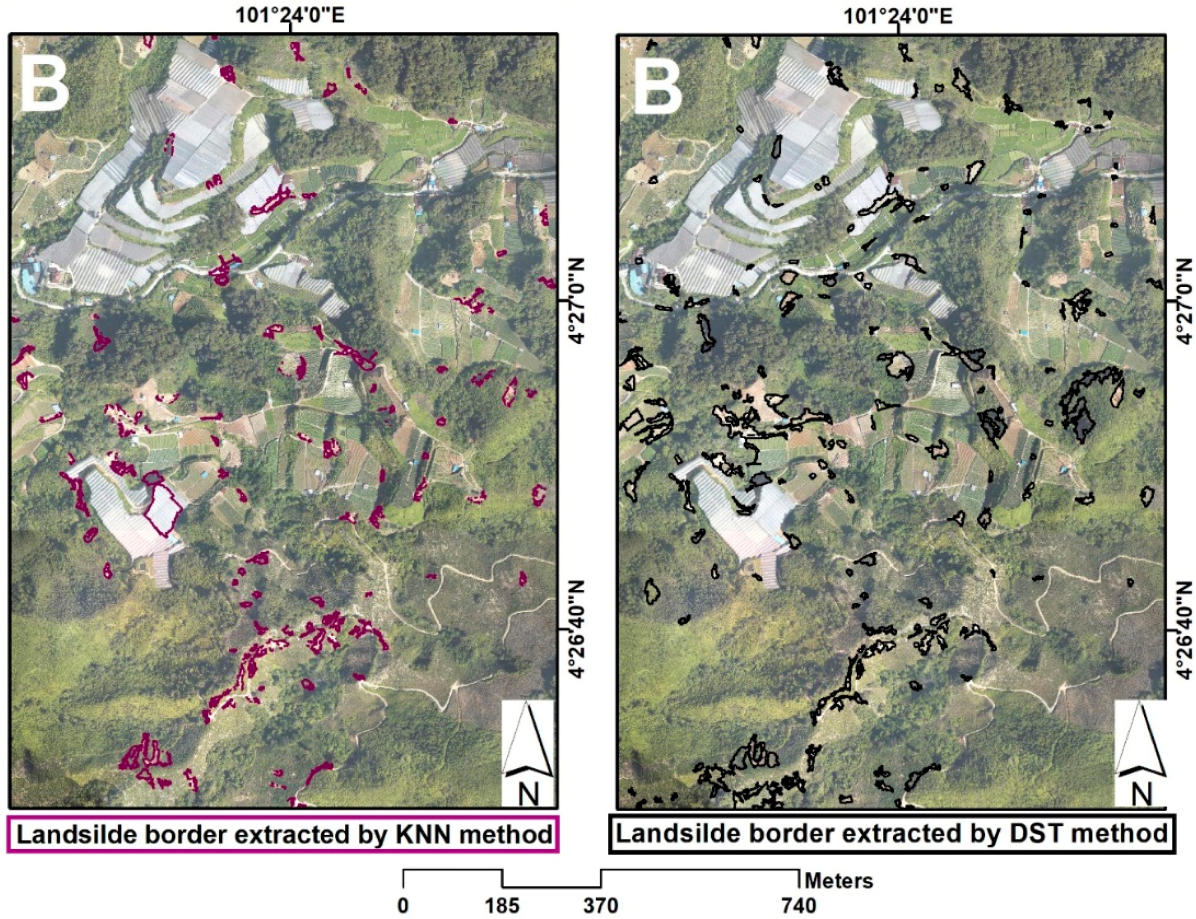
It is necessary to test the transferability of the model developed to other landslide-affected, dense vegetation-cover areas, especially around regions with less anthropogenic activities. In densely vegetated areas such as the Cameron Highlands, landslides are generally covered by a much higher scarp compared to the landslide-free areas. Furthermore, there is a similarity in the characteristics with other land cover classes such as bare soil, cut slope, and manmade classes which pose difficulty in separation among the former classes. Consequently, the results of transferability to validate the proposed method were tested in another part of the study area (testing area), as shown in Figure 6. The results of the consistency in transferability indicate that SVM achieved a consistent accuracy compared with KNN and RF, while the transferability accuracy of RF was better than that of the SVM classifier. Lowered results accuracy shows a decline in results accuracy given the many disadvantages due to similarities in their characteristics as well as the combination of landslide, shape, area, complex topography, and so on [6]. Therefore, this study presented a combination of object-based approaches for landslide mapping. The DST process combined the power of each classifier to derive a more powerful classifier, as shown in Figure 6. DST showed more improvement than SVM, RF, and KNN classifiers separately. Moreover, it is worth observing that the improvement margin of DST is better than that of each classifier. As a result, Figure 6 shows the results of fusion DST, indicating a satisfactory result for landslide identification and delineation between landslides and non-landslides. The results show that the fusion of object-based classifiers in the DST method aided in the identification process of landslides and provided complementary information. The DST decision rule played a great role in resolving the conflicts generated from object-based classifiers. It fuses the benefits of classifiers by adding each classifiers’ information to the other classifiers. It may be inferred that DST offered an improved, high-resolution LiDAR as well as orthophoto images with an acceptable accuracy. In addition, the transferability results show the importance of features from high-resolution LiDAR data, visible bands, and textures features for landslide mapping, shown in Figure 8. In addition, airborne LiDAR data contributed to the detection of the landslide location due to its capability to obtain differences in size and volume of the landslides [70,71].
3.5. Field Investigation
Landslides were identified with the aid of a handheld GPS device in the field investigation, which was carried out to validate the proposed method (GeoExplorer 6000), as illustrated in Figure 9. The information on the pattern, deposition, source area, landslide extent, run out, and volume was obtained from the field measurements, which validated the reliability of the produced landslide map. Based on the field investigation studies, the landslides identified in the proposed method are consistent and accurate. Therefore, this method has the potential to accurately identify landslide locations, differentiate between landslides and non-landslides, as well as yield a reasonable and acceptable landslide inventory map for the Cameron Highlands in Malaysia. In addition, government agencies and land use planners can use the produced results of this study to identify safe regions for inhabitants and update urban planning strategies. Such data can decrease the requirements for performing field surveys by agencies such as departments of surveying.
3.6. Assessing Accuracy
Many established methods of assessing the accuracy of remote sensing products are available in the research domain [72]. In this study, the accuracy assessment was conducted based on quantitative and qualitative (i.e., confusion matrix and precision/recall methods) for the determination of classification accuracy of one or all categories. Firstly, the confusion matrix was derived from comparison between reference image pixels and the classified image pixels. The Kappa coefficient was extracted from the confusion matrix. Thus, this coefficient is calculated as shown in Equation (9):
where denotes the ratio of correctly classified areas, while represents the proportion of agreement expected by chance.
The results of the confusion matrix model were used to evaluate the pixel coverage for detecting landslides in a qualitative assessment approach. In this model, the landslide areas were compared with real landslide areas in the field. This indicates that the degree of precision in delineated landslide segments were resolved. Based on the results, it was observed that out of all the standalone object-based classifiers, the SVM classifier achieved user accuracy up to 80.57% and delineated the exact border of the individual landslide. This result was followed by RF and KNN classifiers with 78.57% and 75.96%, respectively, for training area (A), in addition to 79.89%, 77.27%, and 72.68% for testing area (B), respectively (see Table 5 and Table 6). However, the DST fusion method improved the qualitative accuracy of the standalone classifier with 84.6% and 83.16% for subsets A and B, respectively, as shown in Table 5 and Table 6. Therefore, based on the accuracy assessment measurements, it was observed that fusion DST enhanced the landslide detection analysis quantitatively and qualitatively by 10% and 4%, respectively.
In order to obtain the results for evaluation of pixel coverage for quantitatively detecting landslides, the confusion matrix was employed to validate the performance of classifiers for both subsets (i.e., training area and testing area). The findings of SVM, RF, and KNN for both subsets showed 86.98%, 87.69%, and 88.70%, respectively, for training area (A) and 86.83%, 88.53%, and 89.58% for testing area (B), respectively (see Table 5 and Table 6). On the other hand, the quantitative assessment of the standalone classifier derived from the DST fusion method was enhanced, with results of 90.02% and 91.1% for subsets A and B, respectively (shown in Table 5 and Table 6). The accuracy assessment measurements showed that the fusion DST improved the detection of landslides. Therefore, the proposed method was shown to be effective and may be applied to other regions exhibiting similar conditions to the present study. This improvement is attributed to the proposed methodology, which includes: optimized techniques, capability of LiDAR drive data, and texture features.
Secondly, the precision/recall method is one of the renowned methods for quantitative accuracy assessment. This proposed method was evaluated using field observations in each block, as shown in Equations (10)–(12) [69,70,71,72]:
where the number of correctly detected landslides is referred to as true positive (TP), while the undetected landslides are referred as the false negative (FN). Usually, an FP is identified as a pixel that is falsely recognized as a landslide. The α is a non-negative scalar set to 0.5 in this regard, as suggested by Liu et al. [70]. Furthermore, the success rate is computed using another equation to estimate the successful counted rate achievable by dividing segmented numbers over total trees.
The precision/recall method was used to measure the accuracy of landslide detection quantitatively. The real number of landslide events were recorded using field surveying as a reference. Thereafter, each classification result was compared in order to observe the inventory map. Landslides are regarded as correct if they are recognized in segments by larger or smaller sizes of segment borders. The major idea in landslide counting is in having at least one segment in an occurred landslide, whereby the area of the landslide should not be significant in the mentioned assessment.
F-measure represents the overall accuracy in counting landslide detection, showing consistency in the result of the trained area (subset A) and the tested area (subset B) for all of the classifiers applied. Table 7 represents the number of landslides detected and counted based on previous landslide occurrence. Moreover, the RF classifier recorded the lowest accuracy in landslide detection (72% and 70% for subsets A and B, respectively), followed by the KNN classifier which showed slightly higher accuracy than RF (75% and 73% for subsets A and B, respectively), as shown in Table 7. However, SVM indicated the highest accuracy among all standalone classification methods before fusion, which gained 77% for both study areas. It is apparent that fusion DST has overtaken all three applied classifiers in terms of the outstanding accuracy for landslide counting of 88% in both subsets. Basically, it has been proven that an applied fusion DST technique can quantitatively improve the accuracy of landslide detection.
The use of the DST technique guarantees significant improvement of the detection accuracies. Each of the various classification classifiers in existence has its own merits and demerits. Therefore, the proposed DST utilized in this research showed improved accuracy. Furthermore, optimized techniques for segmentation parameters and feature selection with the assistance of high-resolution LiDAR, visible bands, and texture features contributed to the simplification of the development of the current research and the improvement of the transferability model [67].
The proposed method was developed in the training area and validated in another part of the study area (test area), and as a result, better accuracy was achieved.
4. Conclusions
The optimization of segmentation parameters is an important process used to improve computational efficiency and model performance with different spatial subsets. This process was conducted in the Cameron Highlands area. An essential feature selection process was used to improve the classification accuracy and the computational efficiency in the proposed methodology. An object-based approach was applied using RF, SVM, and KNN techniques. The accuracies achieved in the classification using SVM was observed to be better than the accuracies achieved using KNN and RF, for both training and testing areas. However, the misclassifications of these results should also be taken into account. Thus, the present study demonstrates a fusion of object-based classifiers for detecting landslides using the DST method. The employed DST method fused the results of the classifiers to generate a more accurate landslide inventory map. A more accurate result was observed in the proposed DST method, which was indicated by an improvement in landslide detection over object-based SVM, RF, and KNN classifiers, respectively. This success is justified by the complementary contribution of object-based approaches. In contrast to previous approaches, the main merit of this approach lies in its simplicity and computational efficiency. It also demonstrated that the results of this method were more robust and yielded higher detection accuracy. The authors of the present study feel confident that this detection method will be immensely helpful in mapping landslide inventories and hazard assessment in landslide-prone environments.
Author Contributions
M.R.M. and B.P. performed literature research, assisted in results compiling and developed the figures and writing the manuscript. H.M.R. and B.P. assisted in results compiling. B.P. supervised the research work, field data collection with different agencies, collected field data, processed the field data and writing the entire structure of the manuscript and proofread the content.
Funding
This research is supported by UTS grant number 321740.2232335.
Acknowledgments
The authors would like to thank three anonymous reviewers and Editorial comments by Filippo Catani for their critical review, which helped us to improve the quality of the manuscript.
Conflicts of Interest
The authors declare no conflict of interest.
References
- Galli, M.; Ardizzone, F.; Cardinali, M.; Guzzetti, F.; Reichenbach, P. Comparing landslide inventory maps. Geomorphology 2008, 94, 268–289. [Google Scholar] [CrossRef]
- Pradhan, B.; Mezaal, M.R. Optimized Rule Sets for Automatic Landslide Characteristic Detection in a Highly Vegetated Forests. In Laser Scanning Applications in Landslide Assessment; Springer: New York, NY, USA, 2017; pp. 51–68. [Google Scholar]
- Chen, W.; Li, X.; Wang, Y.; Chen, G.; Liu, S. Forested landslide detection using LiDAR data and the random forest algorithm: A case study of the Three Gorges, China. Remote Sens. Environ. 2014, 152, 291–301. [Google Scholar] [CrossRef]
- Pradhan, B.; Jebur, M.N.; Shafri, H.Z.M.; Tehrany, M.S. Data fusion technique using wavelet transform and taguchi methods for automatic landslide detection from airborne laser scanning data and quick bird satellite imagery. IEEE Trans. Geosci. Remote Sens. 2016, 54, 1610–1622. [Google Scholar] [CrossRef]
- Li, M.; Ma, L.; Blaschke, T.; Cheng, L.; Tiede, D. A systematic comparison of different object-based classification techniques using high spatial resolution imagery in agricultural environments. Int. J. Appl. Earth Obs. Geoinf. 2016, 49, 87–98. [Google Scholar] [CrossRef]
- Mezaal, M.R.; Pradhan, B.; Sameen, M.I.; Mohd Shafri, H.Z.; Yusoff, Z.M. Optimized Neural Architecture for Automatic Landslide Detection from High-Resolution Airborne Laser Scanning Data. Appl. Sci. 2017, 7, 730. [Google Scholar] [CrossRef]
- McKean, J.; Roering, J. Objective landslide detection and surface morphology mapping using high-resolution airborne laser altimetry. Geomorphology 2004, 57, 331–351. [Google Scholar] [CrossRef]
- Van Westen, C.J.; Castellanos, E.; Kuriakose, S.L. Spatial data for landslide susceptibility, hazard, and vulnerability assessment, an overview. Eng. Geol. 2008, 102, 112–131. [Google Scholar] [CrossRef]
- Chen, R.-F.; Lin, C.-W.; Chen, Y.-H.; He, T.-C.; Fei, L.-Y. Detecting and characterizing active thrust fault and deep-seated landslides in dense forest areas of Southern Taiwan Using Airborne LiDAR DEM. Remote Sens. 2015, 7, 15443–15466. [Google Scholar] [CrossRef]
- Mojaddadi, H.; Pradhan, B.; Nampak, H.; Ahmad, N.; Ghazali, A.H.B. Ensemble machine-learning-based geospatial approach for flood risk assessment using multi-sensor remote-sensing data and GIS. Geomat. Nat. Hazards Risk 2017, 8, 1080–1102. [Google Scholar] [CrossRef]
- Guzzetti, F.; Mondini, A.C.; Cardinali, M.; Fiorucci, F.; Santangelo, M.; Chang, K.-T. Landslide inventory maps: New tools for an old problem. Earth-Sci. Rev. 2012, 112, 42–66. [Google Scholar] [CrossRef]
- Blaschke, T. Object based image analysis for remote sensing. ISPRS J. Photogramm. Remote Sens. 2010, 65, 2–16. [Google Scholar] [CrossRef]
- Moosavi, V.; Talebi, A.; Shirmohammadi, B. Producing a landslide inventory map using pixel-based and object-oriented approaches optimized by Taguchi method. Geomorphology 2014, 204, 646–656. [Google Scholar] [CrossRef]
- Zeng, Y.; Zhang, J.; Van Genderen, J. Comparison and analysis of remote sensing data fusion techniques at feature and decision levels. In Proceedings of the ISPRS Mid-Term Symposium 2006 Remote Sensing: From Pixels to Processes, Enschede, The Netherlands, 8–11 May 2006. [Google Scholar]
- Rottensteiner, F.; Trinder, J.; Clode, S.; Kubik, K. Using the Dempster-Shafer method for the fusion of LIDAR data and multi-spectral images for building detection. Inf. Fusion 2005, 6, 283–300. [Google Scholar] [CrossRef]
- Jiang, D.; Zhuang, D.; Fu, J.; Huang, Y. Survey of multispectral image fusion techniques in remote sensing applications. In Image Fusion and Its Applications; INTECH Open Access Publisher: New York, NY, USA, 2011. [Google Scholar]
- Kabolizade, M.; Ebadi, H.; Ahmadi, S. An improved snake model for automatic extraction of buildings from urban aerial images and LiDAR data. Comput. Environ. Urban Syst. 2010, 34, 435–441. [Google Scholar] [CrossRef]
- Bellenger, A.; Gatepaille, S. Uncertainty in ontologies, Dempster-shafer theory for data fusion applications. arXiv, 2011; arXiv:1106.3876. [Google Scholar]
- Yonghong, A.J.; Deren, B.L. Feature fusion based on Dempster-Shafer’s evidential reasoning for I mage texture classification. In Proceedings of the Remote Sensing of Atmospheric Environment: WG III/8, Istanbul, Turkey, 12–23 July 2004. [Google Scholar]
- Singh, R.; Vatsa, M.; Noore, A.; Singh, S.K. Dempster-Shafer theory based classifier fusion for improved fingerprint verification performance. In Computer Vision, Graphics and Image Processing; Lecture Notes in Computer Science; Springer: Berlin/Heidelberg, Germany, 2006; Volume 4338, pp. 941–949. [Google Scholar]
- Fontani, M.; Bianchi, T.; De Rosa, A.; Piva, A.; Barni, M. A Dempster-Shafer framework for decision fusion in image forensics. In Proceedings of the 2011 IEEE International Workshop on Information Forensics and Security (WIFS), Iguacu Falls, Brazil, 29 November–2 December 2011; pp. 1–6. [Google Scholar]
- Althuwaynee, O.F.; Pradhan, B.; Lee, S. Application of an evidential belief function model in landslide susceptibility mapping. Comput. Geosci. 2012, 44, 120–135. [Google Scholar] [CrossRef]
- Bui, D.T.; Pradhan, B.; Lofman, O.; Revhaug, I.; Dick, O.B. Spatial prediction of landslide hazards in Hoa Binh province (Vietnam), a comparative assessment of the efficacy of evidential belief functions and fuzzy logic models. CATENA 2012, 96, 28–40. [Google Scholar] [CrossRef]
- Mohammady, M.; Pourghasemi, H.R.; Pradhan, B. Landslide susceptibility mapping at Golestan Province, Iran: A comparison between frequency ratio, Dempster–Shafer, and weights-of-evidence models. J. Asian Earth Sci. 2012, 61, 221–236. [Google Scholar] [CrossRef]
- Pradhan, B.; Abokharima, M.H.; Jebur, M.N.; Tehrany, M.S. Land subsidence susceptibility mapping at Kinta Valley (Malaysia) using the evidential belief function model in GIS. Nat. Hazards 2014, 73, 1019–1042. [Google Scholar] [CrossRef]
- Nampak, H.; Pradhan, B.; Manap, M.A. Application of GIS based data driven evidential belief function model to predict groundwater potential zonation. J. Hydrol. 2014, 513, 283–300. [Google Scholar] [CrossRef]
- Neshat, A.; Pradhan, B. Risk assessment of groundwater pollution with a new methodological framework: Application of Dempster–Shafer theory and GIS. Nat. Hazards 2015, 78, 1565–1585. [Google Scholar] [CrossRef]
- Mezaal, M.R.; Pradhan, B.; Shafri, H.Z.M.; Yusoff, Z.M. Automatic landslide detection using Dempster–Shafer theory from LiDAR-derived data and orthophotos. Geomat. Nat. Hazards Risk 2017, 1–20. [Google Scholar] [CrossRef]
- Heleno, S.; Matias, M.; Pina, P.; Sousa, A.J. Semiautomated object-based classification of rain-induced landslides with VHR multispectral images on Madeira Island. Nat. Hazards Earth Syst. Sci. 2016, 16, 1035–1048. [Google Scholar] [CrossRef] [Green Version]
- Stumpf, A.; Kerle, N. Object-oriented mapping of landslides using Random Forests. Remote Sens. Environ. 2011, 115, 2564–2577. [Google Scholar] [CrossRef]
- Li, X.; Cheng, X.; Chen, W.; Chen, G.; Liu, S. Identification of forested landslides using LiDar data, object-based image analysis, and machine learning algorithms. Remote Sens. 2015, 7, 9705–9726. [Google Scholar] [CrossRef]
- Zhang, Y.; Maxwell, T.; Tong, H.; Dey, V. Development of a supervised software tool for automated determination of optimal segmentation parameters for ecognition. In SPRS TC VII Symposium—100 Years ISPRS, Vienna, Austria, 5–7 July 2010; Wagner, W., Székely, B., Eds.; IAPRS: Vienna, Austria, 2010. [Google Scholar]
- McCalpin, J. Preliminary age classification of landslides for inventory mapping. In Proceedings of the 21st Annual Engineering Geology and Soils Engineering Symposium, Moscow, Idaho, 5–6 April 1984; pp. 99–111. [Google Scholar]
- Pradhan, B.; Lee, S. Regional landslide susceptibility analysis using back-propagation neural network model at Cameron Highland, Malaysia. Landslides 2010, 7, 13–30. [Google Scholar] [CrossRef]
- Samy, I.E.; Marghany, M.M.; Mohamed, M.M. Landslide modelling and analysis using remote sensing and GIS: A case study of Cameron highland, Malaysia. J. Geomat. 2014, 8, 140–147. [Google Scholar]
- Murakmi, S.; Nishigaya, T.; Tien, T.L.; Sakai, N.; Lateh, H.H.; Azizat, N. Development of historical landslide database in Peninsular Malaysia. In Proceedings of the 2014 IEEE 2nd International Symposium on Telecommunication Technologies (ISTT), Langkawi, Malaysia, 24–26 November 2014; pp. 149–153. [Google Scholar]
- Shahabi, H.; Hashim, M. Landslide susceptibility mapping using GIS-based statistical models and Remote sensing data in tropical environment. Sci. Rep. 2015, 5, 9899. [Google Scholar] [CrossRef] [PubMed] [Green Version]
- Miner, A.; Flentje, P.; Mazengarb, C.; Windle, D. Landslide Recognition using LiDAR derived Digital Elevation Models-Lessons learnt from selected Australian examples. In Proceedings of the 11th IAEG Congress of the International Association of Engineering Geology and the Environment, Auckland, New Zealand, 5–10 September 2010. [Google Scholar]
- Martha, T.R.; Kerle, N.; Van Westen, C.J.; Jetten, V.; Kumar, K.V. Segment optimization and data-driven thresholding for knowledge-based landslide detection by object-based image analysis. IEEE Trans. Geosci. Remote Sens. 2011, 49, 4928–4943. [Google Scholar] [CrossRef]
- Olaya, V. Basic land-surface parameters. Dev. Soil Sci. 2009, 33, 141–169. [Google Scholar] [CrossRef]
- Barbarella, M.; Fiani, M.; Lugli, A. Application of LiDAR-derived DEM for detection of mass movements on a landslide. Int. Arch. Photogramm. Remote Sens. Spat. Inf. Sci. 2013, 89–98. [Google Scholar] [CrossRef]
- Dou, J.; Chang, K.-T.; Chen, S.; Yunus, A.P.; Liu, J.-K.; Xia, H.; Zhu, Z. Automatic case-based reasoning approach for landslide detection, integration of object-oriented image analysis and a genetic algorithm. Remote Sens. 2015, 7, 4318–4342. [Google Scholar] [CrossRef]
- Anders, N.S.; Seijmonsbergen, A.C.; Bouten, W. Segmentation optimization and stratified object-based analysis for semi-automated geomorphological mapping. Remote Sens. Environ. 2011, 115, 2976–2985. [Google Scholar] [CrossRef]
- Belgiu, M.; Drǎguţ, L. Comparing supervised and unsupervised multiresolution segmentation approaches for extracting buildings from very high resolution imagery. ISPRS J. Photogramm. Remote Sens. 2014, 96, 67–75. [Google Scholar] [CrossRef] [PubMed]
- Drǎguţ, L.; Tiede, D.; Levick, S.R. ESP, a tool to estimate scale parameter for multiresolution image segmentation of remotely sensed data. Int. J. Geogr. Inf. Sci. 2010, 24, 859–871. [Google Scholar] [CrossRef]
- Genuer, R.; Michel, V.; Eger, E.; Thirion, B. Random Forests based feature selection for decoding fMRI data. In Proceedings of the COMPSTAT 2010–19th International Conference on Computational Statistics, Paris, France, 22–27 August 2010; pp. 1071–1078. [Google Scholar]
- Van Den Eeckhaut, M.; Kerle, N.; Poesen, J.; Hervás, J. Object-oriented identification of forested landslides with derivatives of single pulse LiDAR data. Geomorphology 2012, 173, 30–42. [Google Scholar] [CrossRef]
- Pawłuszek, K.; Borkowski, A. Landslides identification using airborne laser scanning data derived topographic terrain attributes and support vector machine classification. Int. Arch. Photogramm. Remote Sens. Spat. Inf. Sci. 2016, XLI-B8, 145–149. [Google Scholar] [CrossRef]
- Hong, H.; Pradhan, B.; Jebur, M.N.; Bui, D.T.; Xu, C.; Akgun, A. Spatial prediction of landslide hazard at the Luxi area (China) using support vector machines. Environ. Earth Sci. 2016, 75, 40. [Google Scholar] [CrossRef]
- Ballabio, C.; Sterlacchini, S. Support vector machines for landslide susceptibility mapping: The Staffora River Basin case study, Italy. Math. Geosci. 2012, 44, 47–70. [Google Scholar] [CrossRef]
- Mountrakis, G.; Im, J.; Ogole, C. Support vector machines in remote sensing, A review. ISPRS J. Photogramm. Remote Sens. 2011, 66, 247–259. [Google Scholar] [CrossRef]
- Huang, C.; Davis, L.; Townshend, J. An assessment of support vector machines for land cover classification. Int. J. Remote Sens. 2002, 23, 725–749. [Google Scholar] [CrossRef]
- Meyer, D.; Dimitriadou, E.; Hornik, K.; Weingessel, A.; Leisch, F. e1071: Misc Functions of the Department of Statistics (e1071); R Package Version 1.6-4; TU Wien: Vienna, Austria, 2014. [Google Scholar]
- R Development Core Team. R: A Language and Environment for Statistical Computing; The R Foundation for Statistical Computing: Vienna, Austria, 2011; Available online: http://www.R-project.org (accessed on 2 February 2017).
- Liaw, A.; Wiener, M. Classification and regression by randomForest. R News 2002, 2, 18–22. [Google Scholar]
- Chen, T.; Trinder, J.C.; Niu, R. Object-oriented landslide mapping using ZY-3 satellite imagery, random forest and mathematical morphology, for the Three-Gorges Reservoir, China. Remote Sens. 2017, 9, 333. [Google Scholar] [CrossRef]
- Chen, W.; Xie, X.; Wang, J.; Pradhan, B.; Hong, H.; Bui, D.T.; Duan, Z.; Ma, J. A comparative study of logistic model tree, random forest, and classification and regression tree models for spatial prediction of landslide susceptibility. CATENA 2017, 151, 147–160. [Google Scholar] [CrossRef]
- Luque-Baena, R.M.; Elizondo, D.; López-Rubio, E.; Palomo, E.J.; Watson, T. Assessment of geometric features for individual identification and verification in biometric hand systems. Expert Syst. Appl. 2013, 40, 3580–3594. [Google Scholar] [CrossRef]
- Cheng, G.; Guo, L.; Zhao, T.; Han, J.; Li, H.; Fang, J. Automatic landslide detection from remote-sensing imagery using a scene classification method based on BoVW and pLSA. Int. J. Remote Sens. 2013, 34, 45–59. [Google Scholar] [CrossRef]
- Shafer, G. A Mathematical Theory of Evidence; Princeton University Press: Princeton, NJ, USA, 1976. [Google Scholar]
- Bobkowska, K. Analysis of the objects images on the sea using Dempster-Shafer Theory. In Proceedings of the IEEE 2016 17th International Radar Symposium (IRS), Krakow, Poland, 10–12 May 2016; pp. 1–4. [Google Scholar]
- Foley, B.G. A Dempster-Shafer Method for Multi-Sensor Fusion; Air Force Institute of Technology-Graduate School of Engineering & Management: Wright-Patterson AFB, OH, USA, 2012. [Google Scholar]
- Dempster, A.P. Upper and lower probabilities induced by a multivalued mapping. Ann. Math. Stat. 1967, 38, 325–339. [Google Scholar] [CrossRef]
- Mezaal, M.R.; Pradhan, B.; Shafri, H.Z.M.; Mojaddadi, H.; Yusoff, Z.M. Optimized Hierarchical Rule-Based Classification for Differentiating Shallow and Deep-Seated Landslide Using High-Resolution LiDAR Data. In Proceedings of the Global Civil Engineering Conference, Kuala Lumpur, Malaysia, 25–28 July 2017; Springer: Singapore, 2017; pp. 825–848. [Google Scholar]
- Rizeei, H.M.; Saharkhiz, M.A.; Pradhan, B.; Ahmad, N. Soil erosion prediction based on land cover dynamics at the Semenyih watershed in Malaysia using LTM and USLE models. Geocarto Int. 2016, 31, 1158–1177. [Google Scholar] [CrossRef]
- Borghuis, A.; Chang, K.; Lee, H. Comparison between automated and manual mapping of typhoon-triggered landslides from SPOT-5 imagery. Int. J. Remote Sens. 2007, 28, 1843–1856. [Google Scholar] [CrossRef]
- Janowski, A.; Szulwic, J.; Tysiac, P.; Wojtowicz, A. Airborne and mobile laser scanning in measurements of sea cliffs on the southern Baltic. In Proceedings of the International Multidisciplinary Scientific GeoConference Surveying Geology & mining Ecology Management (SGEM), Albena, Bulgaria, 18–24 June 2015; Volume 2, p. 17. [Google Scholar]
- Nyland, R.D. Silviculture: Concepts and Applications; Waveland Press: Long Grove, IL, USA, 2016. [Google Scholar]
- Rizeei, H.M.; Shafri, H.Z.; Mohamoud, M.A.; Pradhan, B.; Kalantar, B. Oil palm counting and age estimation from WorldView-3 imagery and LiDAR data using an integrated OBIA height model and regression analysis. J. Sens. 2017. [Google Scholar] [CrossRef]
- Liu, T.; Yuan, Z.; Sun, J.; Wang, J.; Zheng, N.; Tang, X.; Shum, H.-Y. Learning to detect a salient object. IEEE Trans. Pattern Anal. 2011, 33, 353–367. [Google Scholar] [CrossRef]
- Mezaal, M.R.; Pradhan, B. Data mining-aided automatic landslide detection using airborne laser scanning data in densely forested tropical areas. KJRS 2018, 34, 45–74. [Google Scholar]
- Mezaal, M.R.; Pradhan, B. An improved algorithm for identifying shallow and deep-seated landslides in dense tropical forest from airborne laser scanning data. CATENA 2018, 167, 147–159. [Google Scholar] [CrossRef]
Figure 1.
Proposed methodology of the current study.

Figure 2.
Study area: (A) Training area; and (B) Test site.

Figure 3.
Landslide inventory map for the training site.

Figure 4.
Landslide inventory map for the testing site.

Figure 5.
LiDAR derived data: (A) Digital Surface Model (DSM); (B) Digital Terrain Model (DTM); (C) Intensity; (D) Hillshade; (E) Height; (F) Slope; and (G) Aspect.
Figure 5.
LiDAR derived data: (A) Digital Surface Model (DSM); (B) Digital Terrain Model (DTM); (C) Intensity; (D) Hillshade; (E) Height; (F) Slope; and (G) Aspect.


Figure 6.
Segmentation process using supervised approach (fuzzy-based segmentation parameter (FbSP) optimizer) to detect landslide locations. (A,B) represent the initial segmentation, while (C,D) represent the optimized segmentation.
Figure 6.
Segmentation process using supervised approach (fuzzy-based segmentation parameter (FbSP) optimizer) to detect landslide locations. (A,B) represent the initial segmentation, while (C,D) represent the optimized segmentation.

Figure 7.
The classification results of three classifiers: (yellow polygon) represents support vector machine (SVM), (red polygon) represents random forest (RF), (purple polygon) represents K-nearest neighbor (KNN), and (black polygon) represents Dempster–Shafer theory (DST) for the training area.
Figure 7.
The classification results of three classifiers: (yellow polygon) represents support vector machine (SVM), (red polygon) represents random forest (RF), (purple polygon) represents K-nearest neighbor (KNN), and (black polygon) represents Dempster–Shafer theory (DST) for the training area.

Figure 8.
The classification results of three classifiers: (yellow polygon) represents SVM, (red polygon) represents RF, (purple polygon) represent KNN, and (black polygon) represents DST for the testing Area.
Figure 8.
The classification results of three classifiers: (yellow polygon) represents SVM, (red polygon) represents RF, (purple polygon) represent KNN, and (black polygon) represents DST for the testing Area.


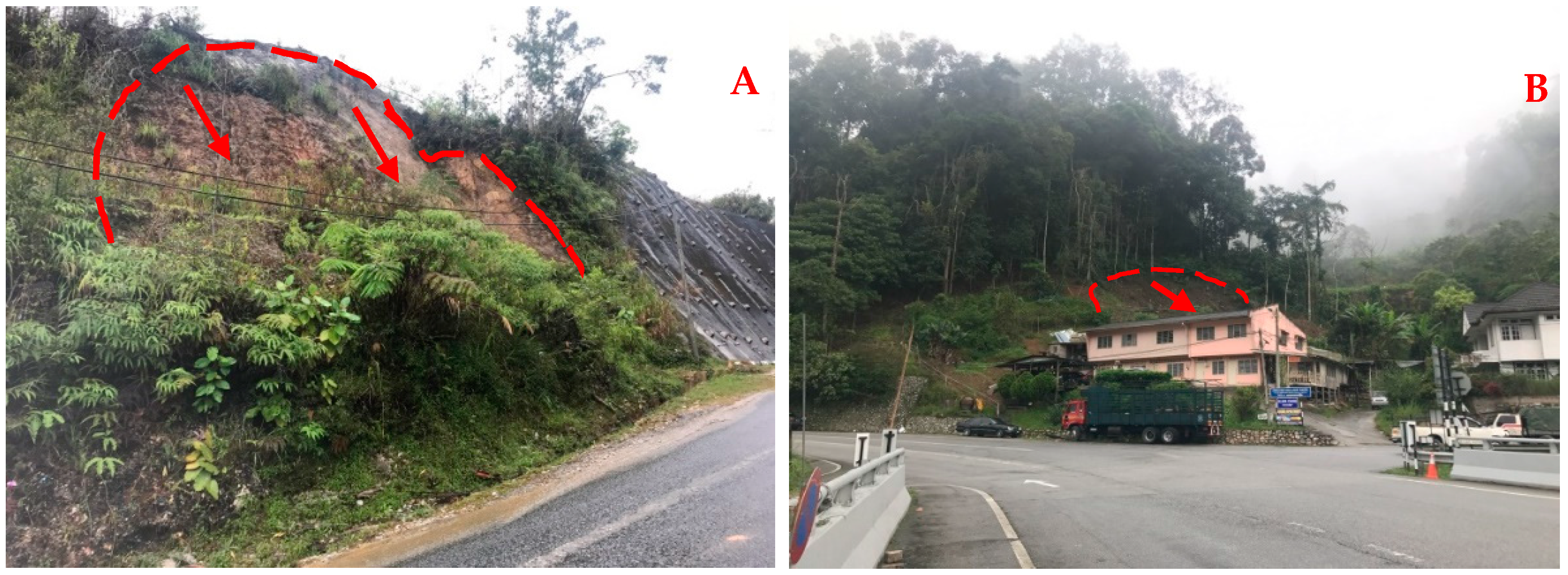
Figure 9.
Field photographs showing landslide locations in the study area: (A) Tanah Rata; and (B) Ringlet.
Figure 9.
Field photographs showing landslide locations in the study area: (A) Tanah Rata; and (B) Ringlet.


Table 1.
Feature selection used in the current research.
| Features Objects | Features Used |
|---|---|
| LiDAR data | Mean and StdDev (Intensity, DEM, DSM, Slope, Aspect, Height) |
| Visible bands | Mean and StdDev (Red, Green, and Blue, Max. diff, and Brightness) |
| Texture features | Four directions, 0°, 45°, 90°, 135° (Gray-level co-occurrence matrix (GLCM) correlation, GLCM Dissimilarity, GLCM angular second moment, GLCM StdDev, GLCM Mean, GLCM Contrast, GLCM Entropy, GLCM Homogeneity, GLDV angular second moment, Grey level difference vector (GLDV) Mean, GLDV Entropy and GLDV Contrast) |
Table 2.
Correlation coefficient between the best feature selection.
| Mean Intensity | GLCM Homogeneity | Mean Slope | Mean Red | Mean DTM | GLCM Contrast | GLCM Dissimilarity | GLCM Angular Second Moment | StdDev Blue | StdDe DTM | |
|---|---|---|---|---|---|---|---|---|---|---|
| Mean intensity | 1 | |||||||||
| GLCM Homogeneity | −0.099 | 1 | ||||||||
| Mean Slope | −0.076 | −0.058 | 1 | |||||||
| Mean Red | −0.011 | −0.103 | 0.046 | 1 | ||||||
| Mean DTM | 0.116 | −0.158 | 0.632 ** | 0.074 | 1 | |||||
| GLCM Contrast | 0.077 | −0.249 ** | 0.003 | 0.958 ** | 0.048 | 1 | ||||
| GLCM Dissimilarity | 0.292 ** | −0.453 ** | −0.060 | 0.790 ** | 0.008 | 0.922 ** | 1 | |||
| GLCM Angular second moment | 0.333 ** | 0.359 ** | −0.075 | −0.007 | −0.046 | 0.010 | 0.042 | 1 | ||
| StdDev Blue | −0.575 ** | 0.181 ** | 0.275 ** | 0.035 | 0.028 | −0.091 | −0.285 ** | −0.055 | 1 | |
| StdDe DTM | 0.139 | −0.004 | −0.129 * | −0.158 * | −0.163 ** | −0.094 | −0.008 | 0.015 | −0.122 | 1 |
** Significant at 0.01 level, * significant at 0.05 level.
Table 3.
Multiresolution segmentation parameters.
| Initial Parameters | Optimal Parameters | |||||
|---|---|---|---|---|---|---|
| No. | Scale | Shape | Compactness | Scale | Shape | Compactness |
| 1 | 50 | 0.1 | 0.1 | 75.52 | 0.4 | 0.5 |
| 2 | 80 | 0.1 | 0.1 | 100 | 0.45 | 0.74 |
Table 4.
Results of feature selection using the correlation-based feature selection (CFS) algorithm.
Table 4.
Results of feature selection using the correlation-based feature selection (CFS) algorithm.
| Feature | Iteration | Rank |
|---|---|---|
| Mean Intensity | 20 | 1 |
| GLCM Homogeneity | 18 | 2 |
| Mean Slope | 20 | 3 |
| GLCM Angular Second Moment | 20 | 4 |
| StdDe DTM | 17 | 5 |
| Mean Red | 20 | 6 |
| Mean DTM | 20 | 7 |
| GLCM Contrast | 18 | 8 |
| GLCM Dissimilarity | 15 | 9 |
| StdDev Blue | 20 | 10 |
Table 5.
Classification assessment (confusion matrices) on the training area.
| Classification Method | Class Name | Ground Truth Points | Total Samples | User Accuracy | Overall Accuracy | Kappa Index | |
|---|---|---|---|---|---|---|---|
| Landslide | Non-Landslides | ||||||
| RF classifier | Landslides | 1917 | 523 | 2440 | 78.57% | 87.69% | 0.63 |
| Non-Landslides | 1089 | 9567 | 10,656 | 89.78% | |||
| SVM classifier | Landslides | 1966 | 474 | 2440 | 80.57% | 86.98% | 0.66 |
| Non-Landslides | 1231 | 9425 | 10,656 | 88.45% | |||
| KNN classifier | Landslides | 1853 | 587 | 2440 | 75.96% | 88.70% | 0.65 |
| Non-Landslides | 891 | 9765 | 10,656 | 91.64% | |||
| DST classifier | Landslides | 2065 | 375 | 2440 | 84.64% | 90.02 | 0.70 |
| Non-Landslides | 931 | 9725 | 10,656 | 91.26% | |||
Table 6.
Classification assessment (confusion matrices) on the testing area.
| Classification Method | Class Name | Ground Truth Points | Total Samples | User Accuracy | Overall Accuracy | Kappa Index | |
|---|---|---|---|---|---|---|---|
| Landslide | Non-Landslides | ||||||
| RF classifier | Landslides | 1759 | 518 | 2277 | 77.27% | 86.83% | 0.61 |
| Non-Landslides | 1023 | 8396 | 9419 | 89.14% | |||
| SVM classifier | Landslides | 1819 | 458 | 2277 | 79.89% | 88.53% | 0.66 |
| Non-Landslides | 883 | 8536 | 9419 | 90.63% | |||
| KNN classifier | Landslides | 1655 | 622 | 2277 | 72.68% | 89.58% | 0.67 |
| Non-Landslides | 596 | 8823 | 9419 | 93.67% | |||
| DST classifier | Landslides | 1894 | 383 | 2277 | 83.18% | 91.1% | 0.73 |
| Non-Landslides | 658 | 8761 | 9419 | 93.01% | |||
Table 7.
Quantitative assessment for both areas.
| Training Area | Testing Area | |||||||
|---|---|---|---|---|---|---|---|---|
| Methods | RF | SVM | KNN | DST | RF | SVM | KNN | DST |
| Inventory | 90 | 90 | 90 | 90 | 129 | 129 | 129 | 129 |
| TP | 67 | 74 | 70 | 84 | 78 | 98 | 81 | 116 |
| FN | 12 | 14 | 35 | 7 | 18 | 12 | 25 | 9 |
| FP | 34 | 26 | 17 | 13 | 41 | 39 | 32 | 20 |
| Precision | 0.66 | 0.74 | 0.80 | 0.87 | 0.66 | 0.72 | 0.72 | 0.85 |
| Recall | 0.85 | 0.84 | 0.67 | 0.92 | 0.81 | 0.89 | 0.76 | 0.93 |
| F-measure | 0.72 | 0.77 | 0.75 | 0.88 | 0.70 | 0.77 | 0.73 | 0.88 |
© 2018 by the authors. Licensee MDPI, Basel, Switzerland. This article is an open access article distributed under the terms and conditions of the Creative Commons Attribution (CC BY) license (http://creativecommons.org/licenses/by/4.0/).
Share and Cite
MDPI and ACS Style
Mezaal, M.R.; Pradhan, B.; Rizeei, H.M. Improving Landslide Detection from Airborne Laser Scanning Data Using Optimized Dempster–Shafer. Remote Sens. 2018, 10, 1029. https://0-doi-org.brum.beds.ac.uk/10.3390/rs10071029
AMA Style
Mezaal MR, Pradhan B, Rizeei HM. Improving Landslide Detection from Airborne Laser Scanning Data Using Optimized Dempster–Shafer. Remote Sensing. 2018; 10(7):1029. https://0-doi-org.brum.beds.ac.uk/10.3390/rs10071029
Chicago/Turabian StyleMezaal, Mustafa Ridha, Biswajeet Pradhan, and Hossein Mojaddadi Rizeei. 2018. "Improving Landslide Detection from Airborne Laser Scanning Data Using Optimized Dempster–Shafer" Remote Sensing 10, no. 7: 1029. https://0-doi-org.brum.beds.ac.uk/10.3390/rs10071029
Note that from the first issue of 2016, this journal uses article numbers instead of page numbers. See further details here.