Mapping up-to-Date Paddy Rice Extent at 10 M Resolution in China through the Integration of Optical and Synthetic Aperture Radar Images

 , ,
, ,
Abstract
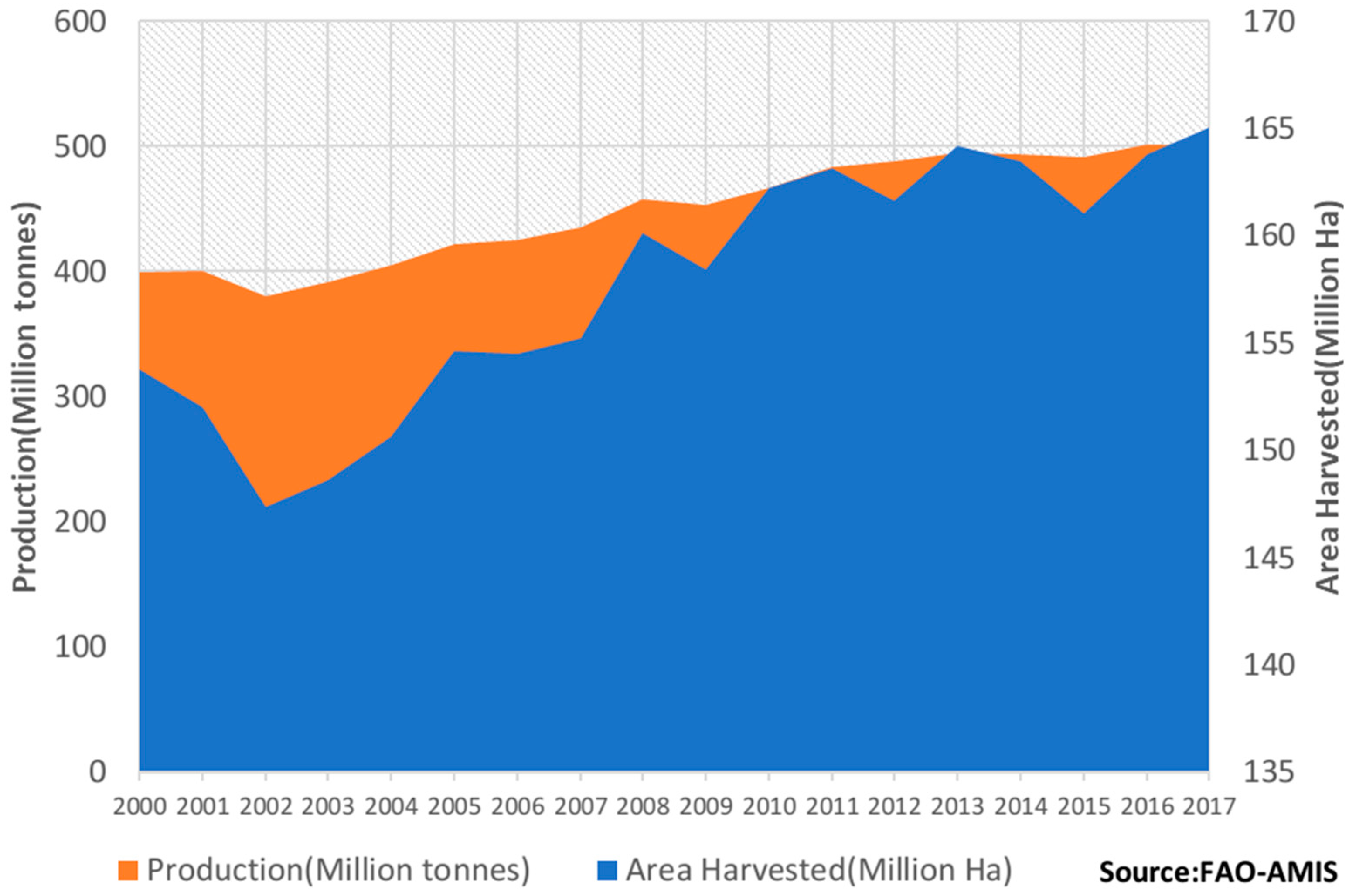
:1. Introduction
2. Materials
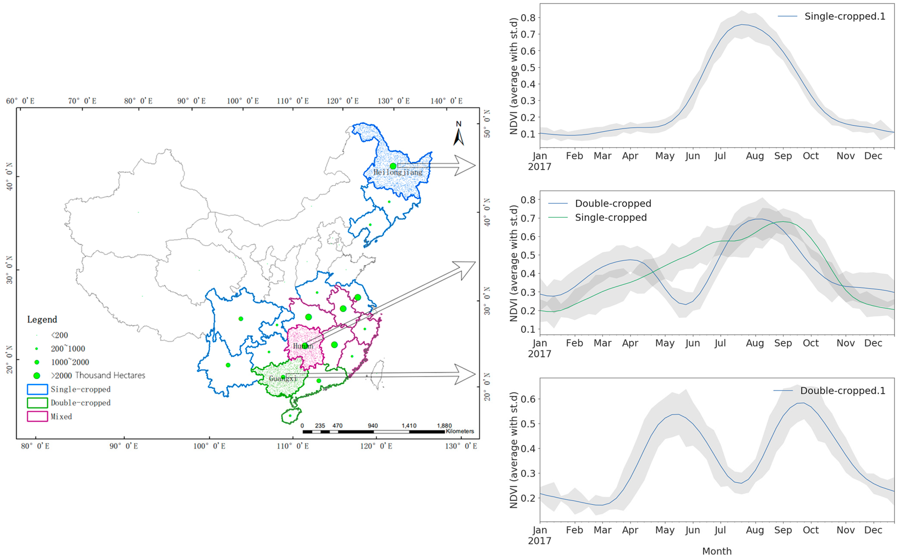
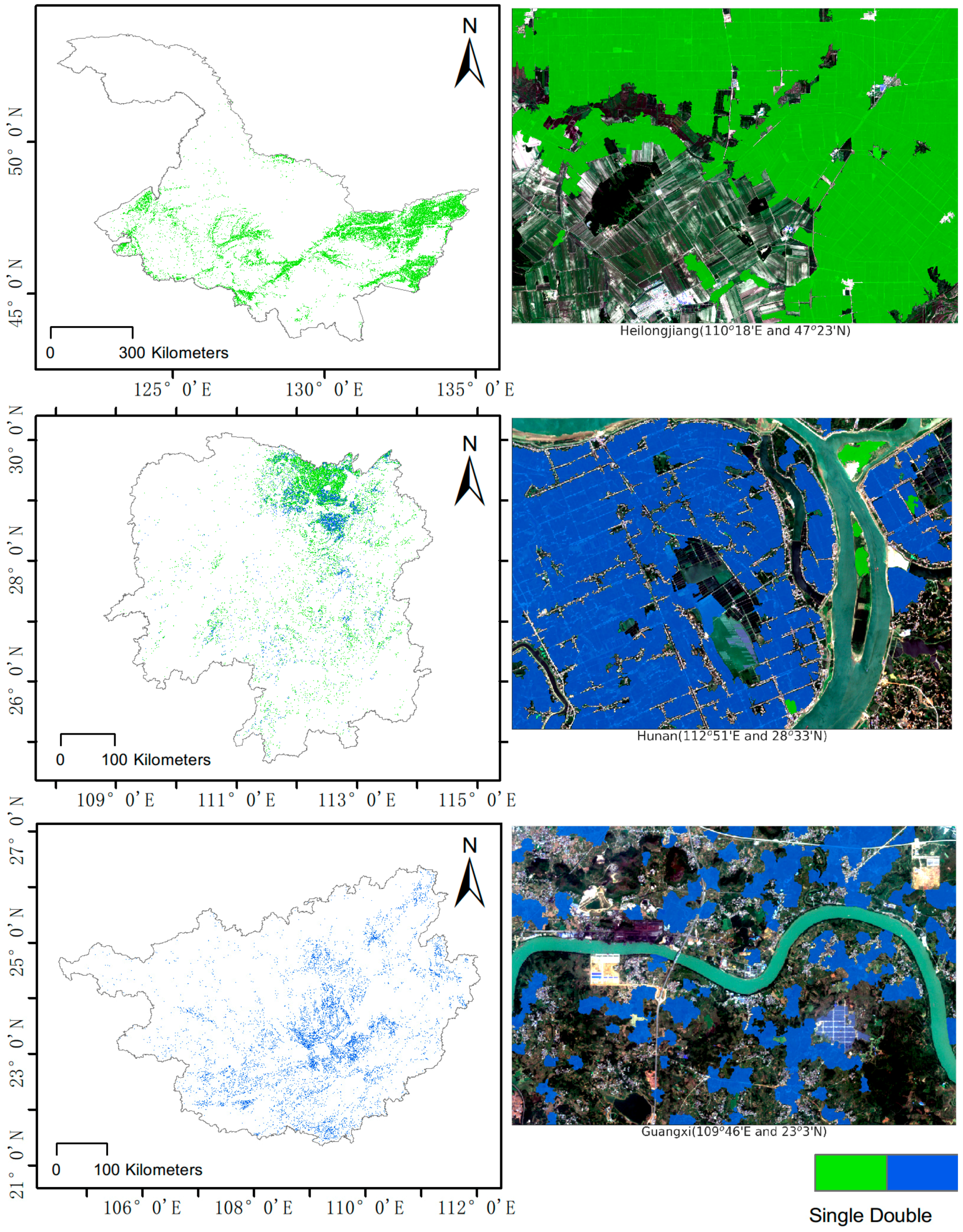
2.1. Study Area
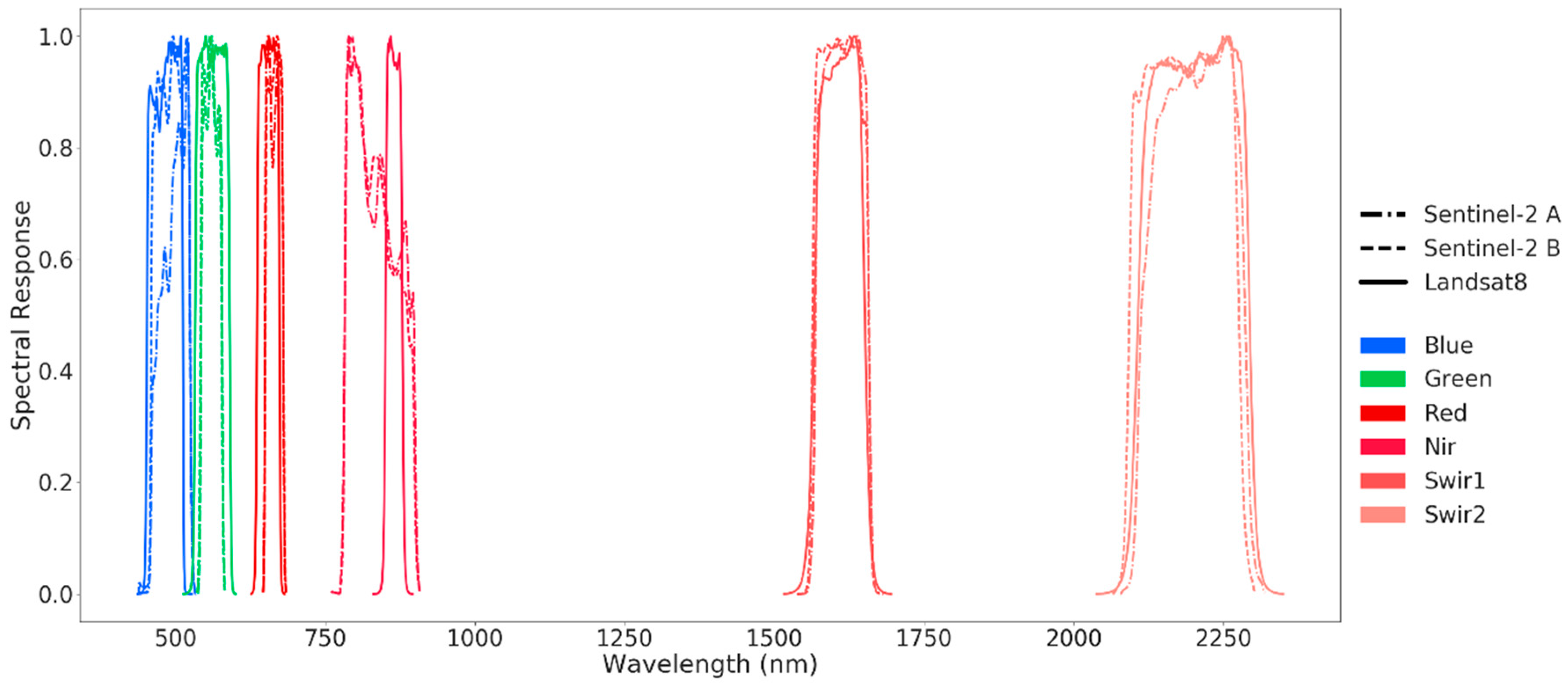
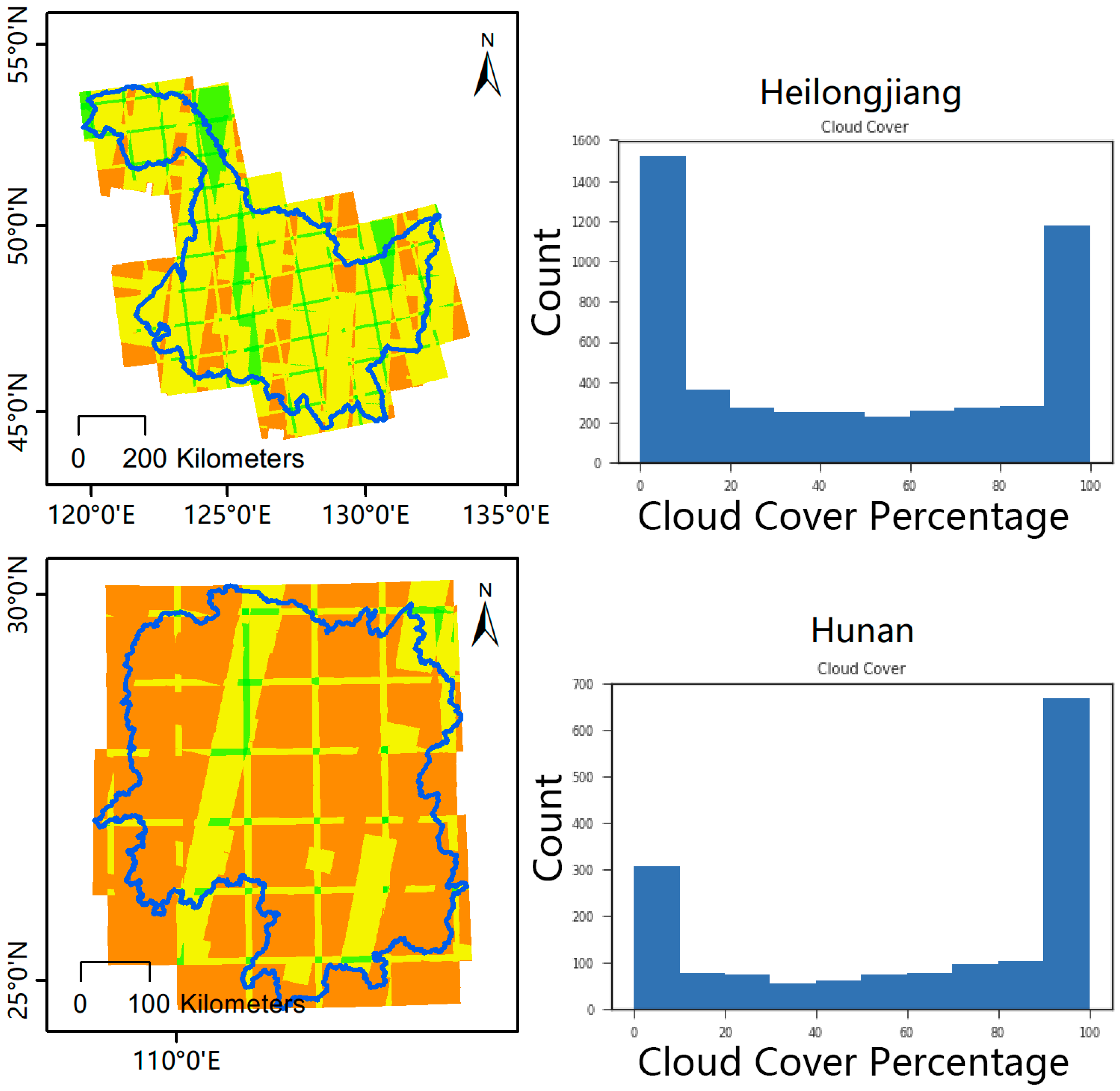
2.2. Data and Preprocessing
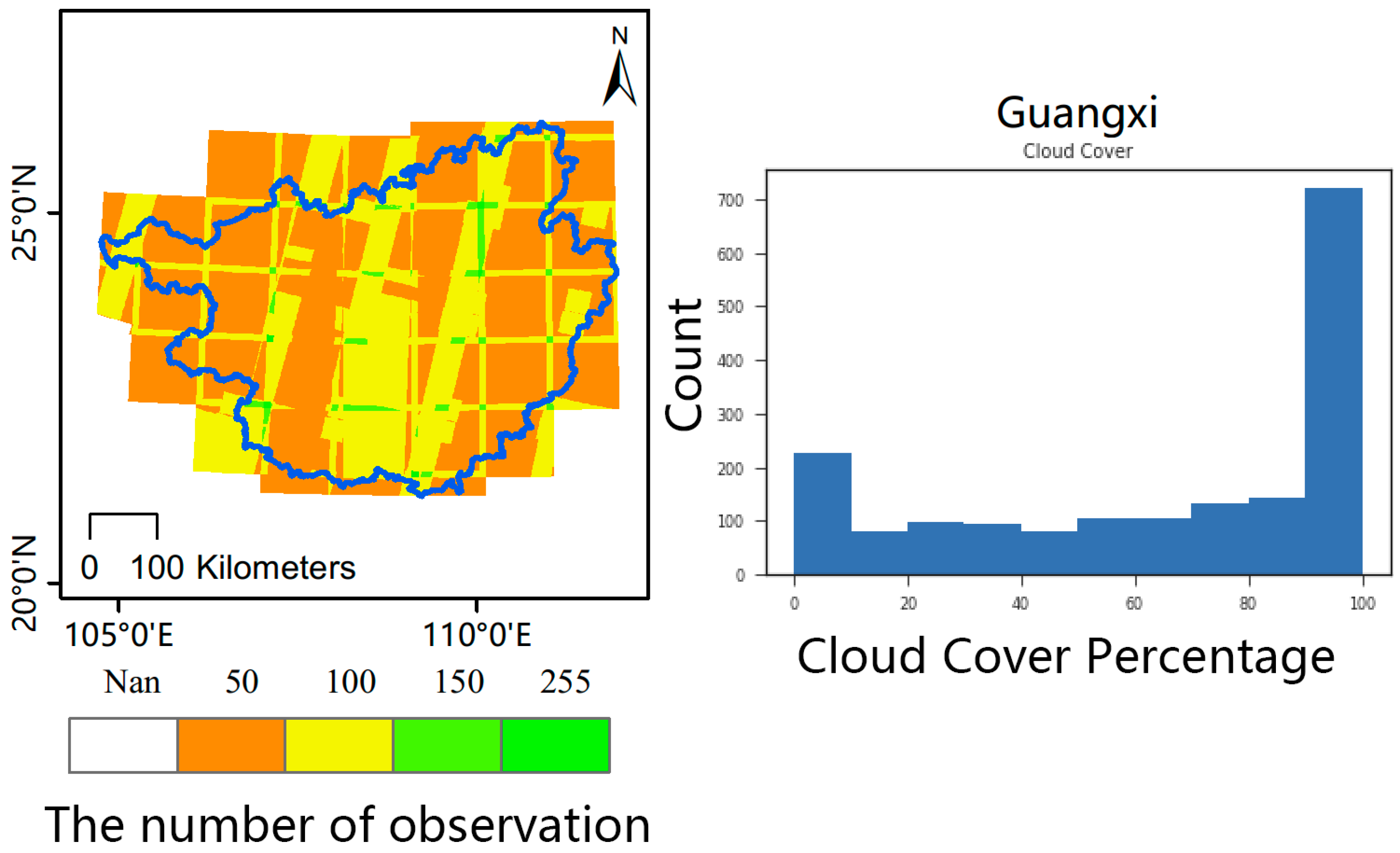
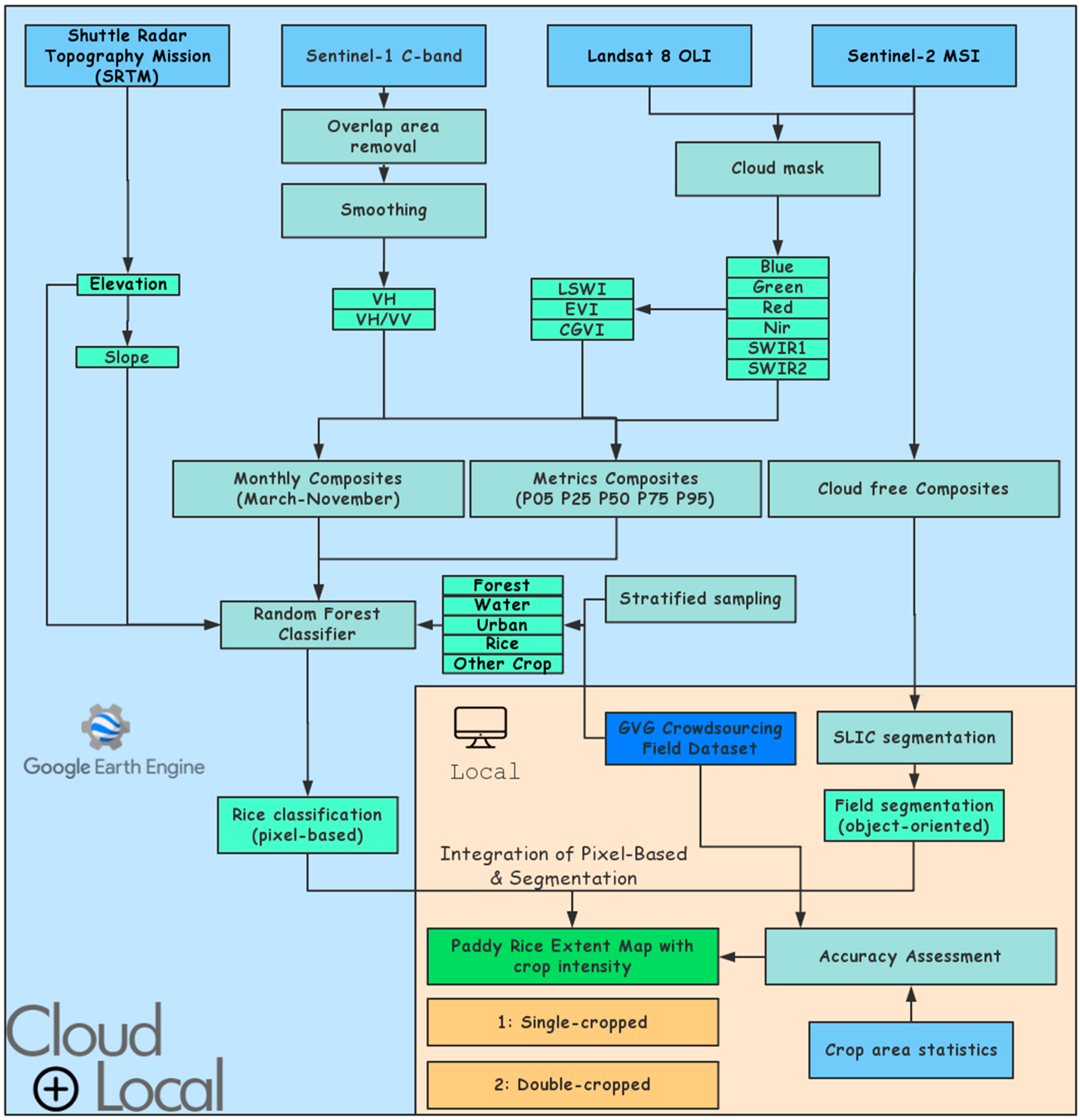
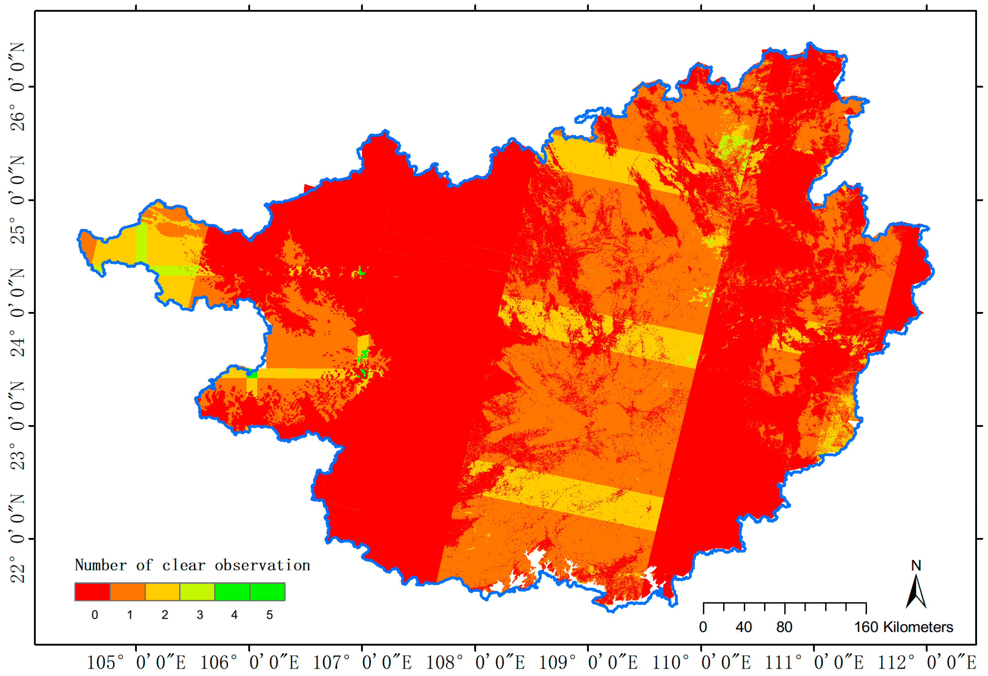
2.2.1. Cloud-Free Optical Imagery Composition
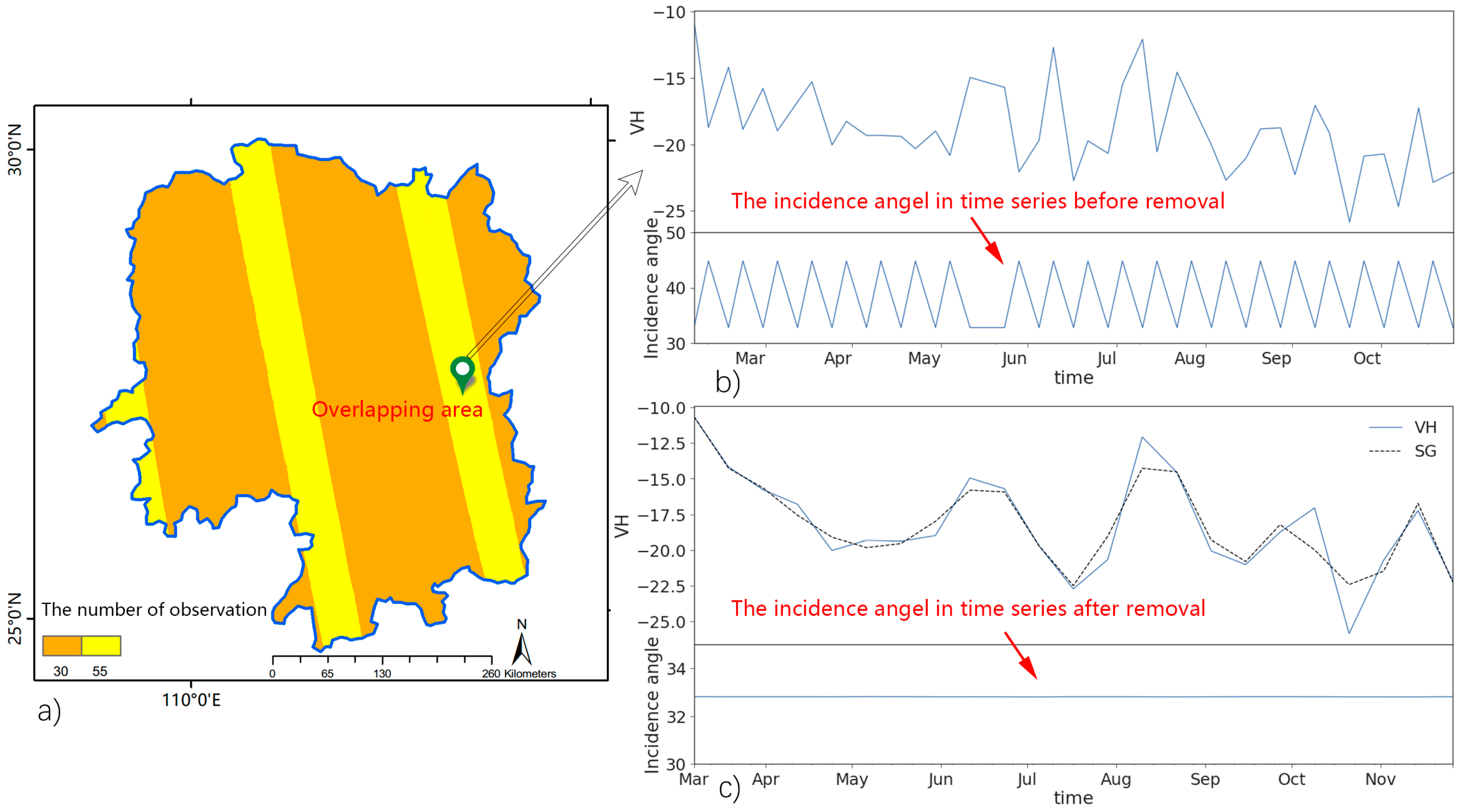
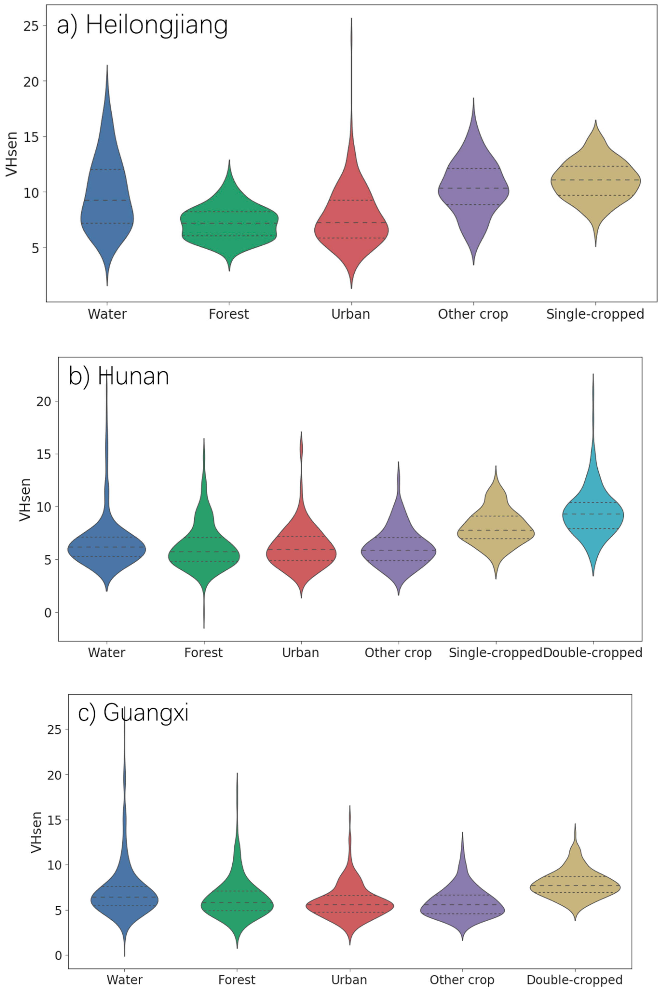
2.2.2. Synthetic Aperture Radar (SAR) Image Preprocessing
- Orbit file application (using restituted orbits)
- Thermal noise removal
- Radiometric calibration
- Terrain correction (orthorectification) using SRTM 30 or ASTER DEM for areas greater than ±60° latitude, where SRTM was not available.
2.2.3. Auxiliary Data
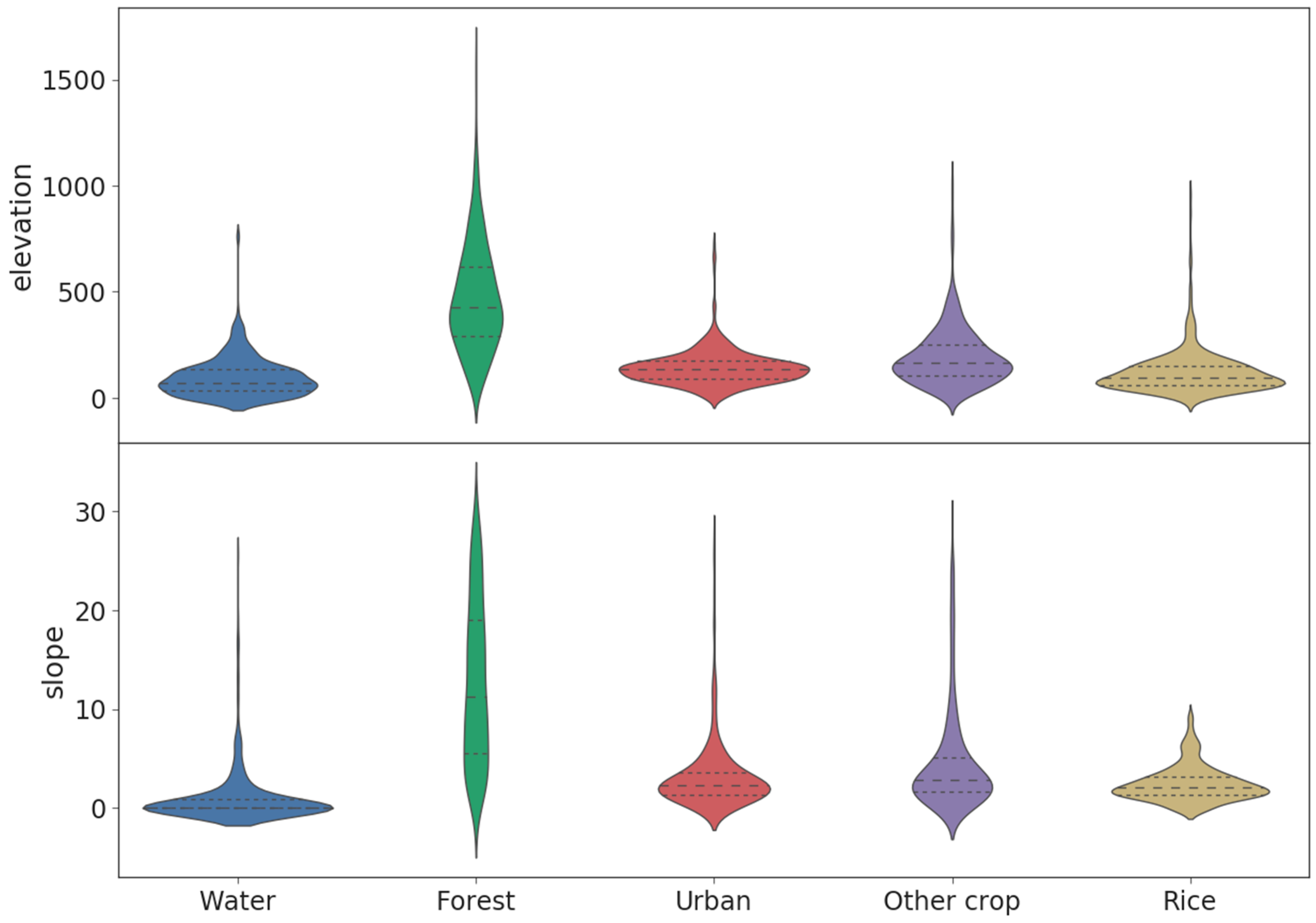
Topographic Data
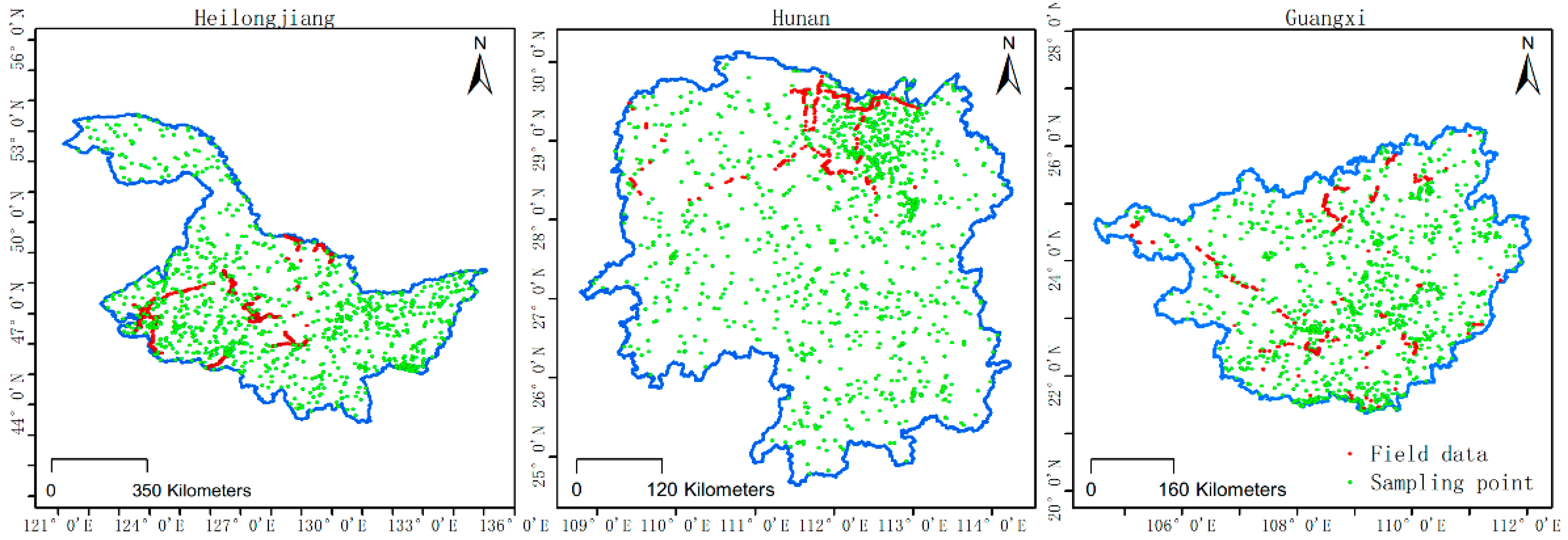
Stratified Random Sample Points
Field Data
3. Methodology
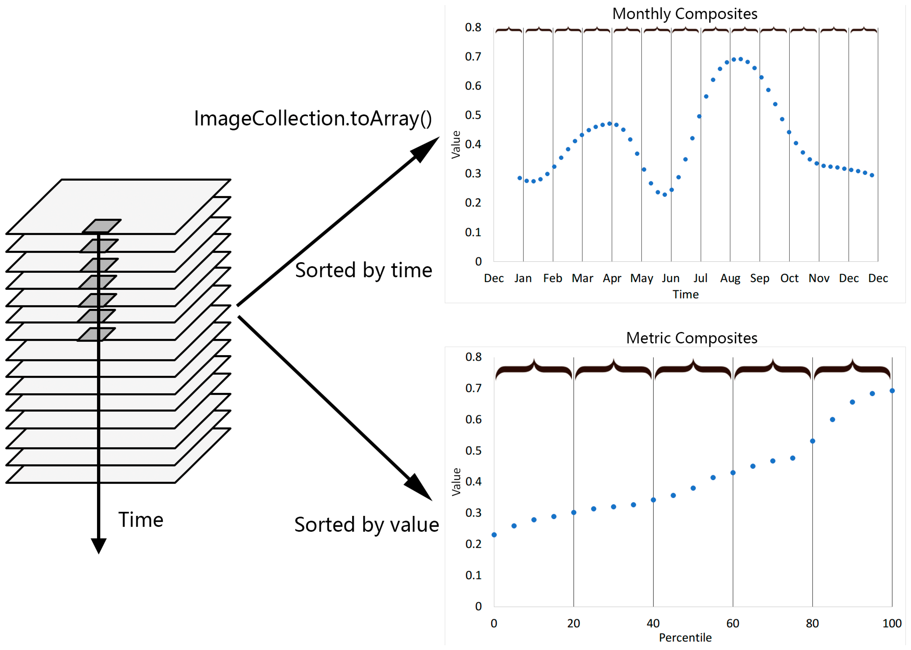
3.1. Monthly and Metric Composites
3.2. Pixel-Based Classifier: Random Forest (RF)
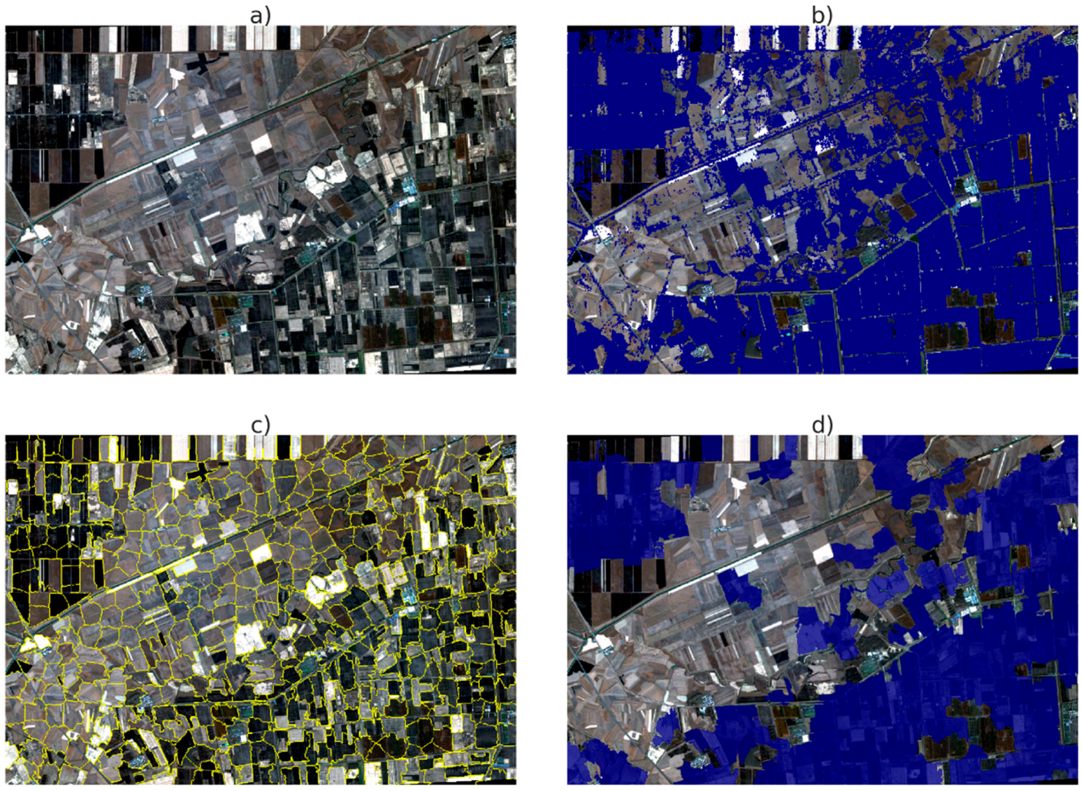
3.3. Simple Linear Iterative Clustering (SLIC) Superpixel Segmentation
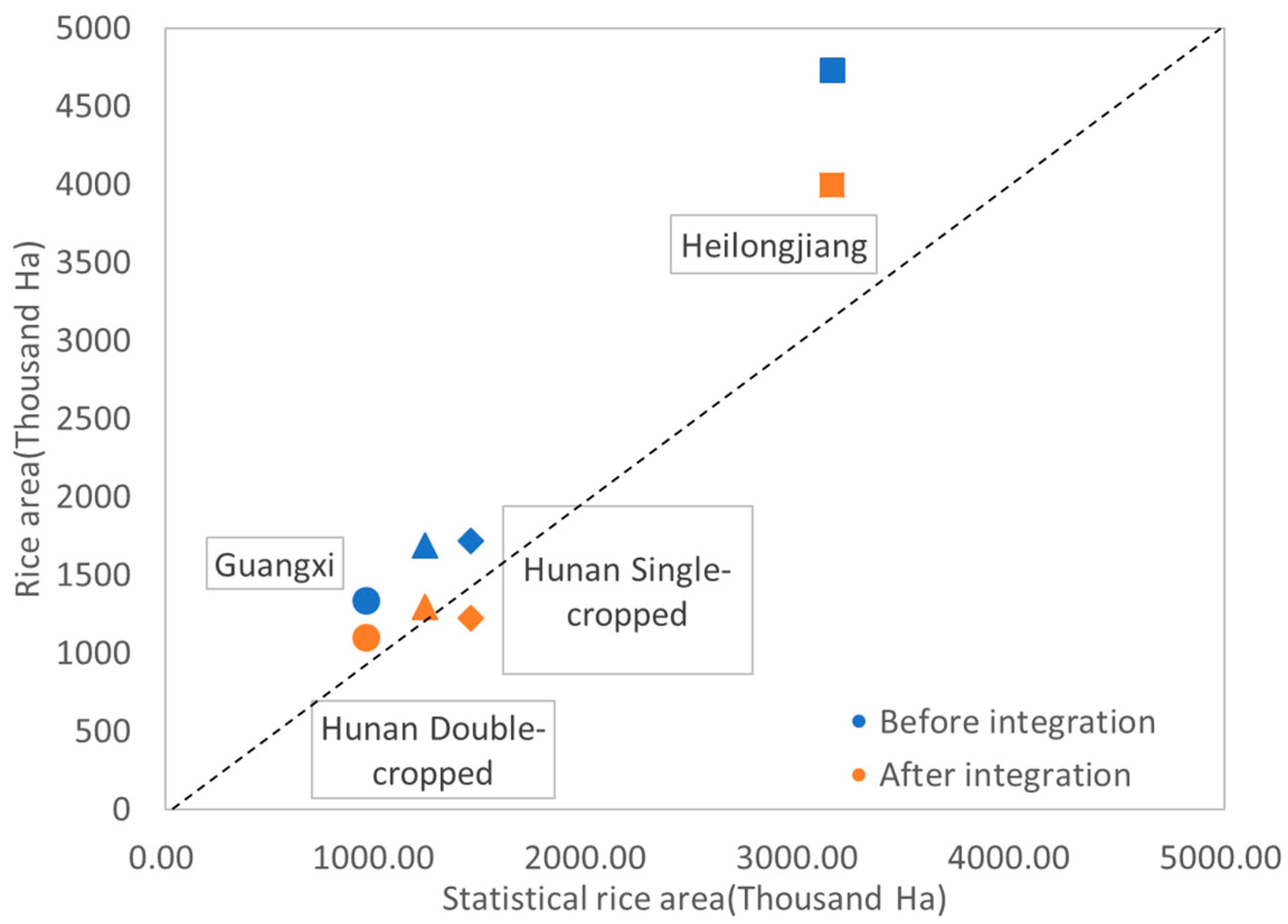
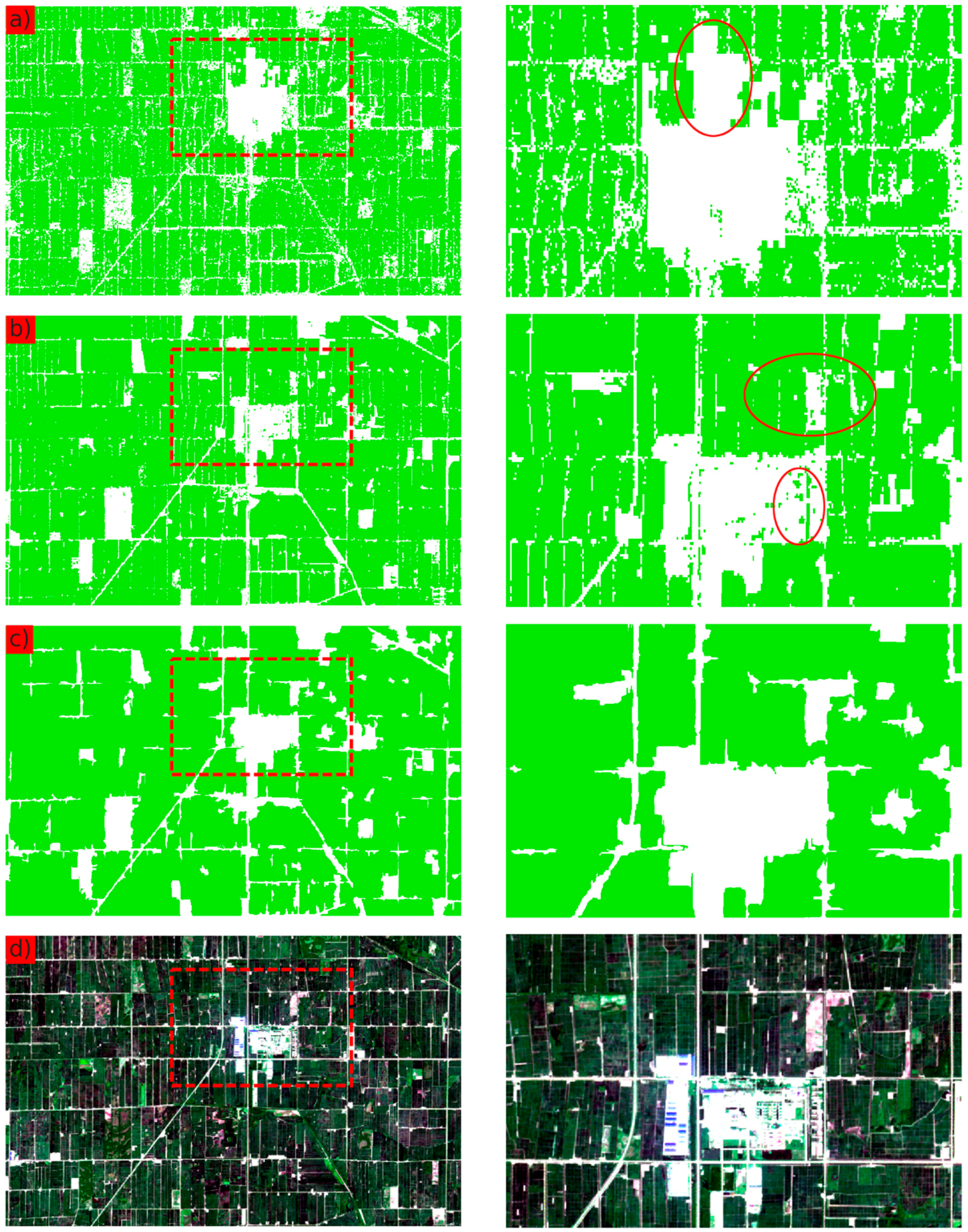
3.4. Integration of the Pixel-Based Classification and the Object-Based Segmentation
3.5. Accuracy Assessment
4. Results
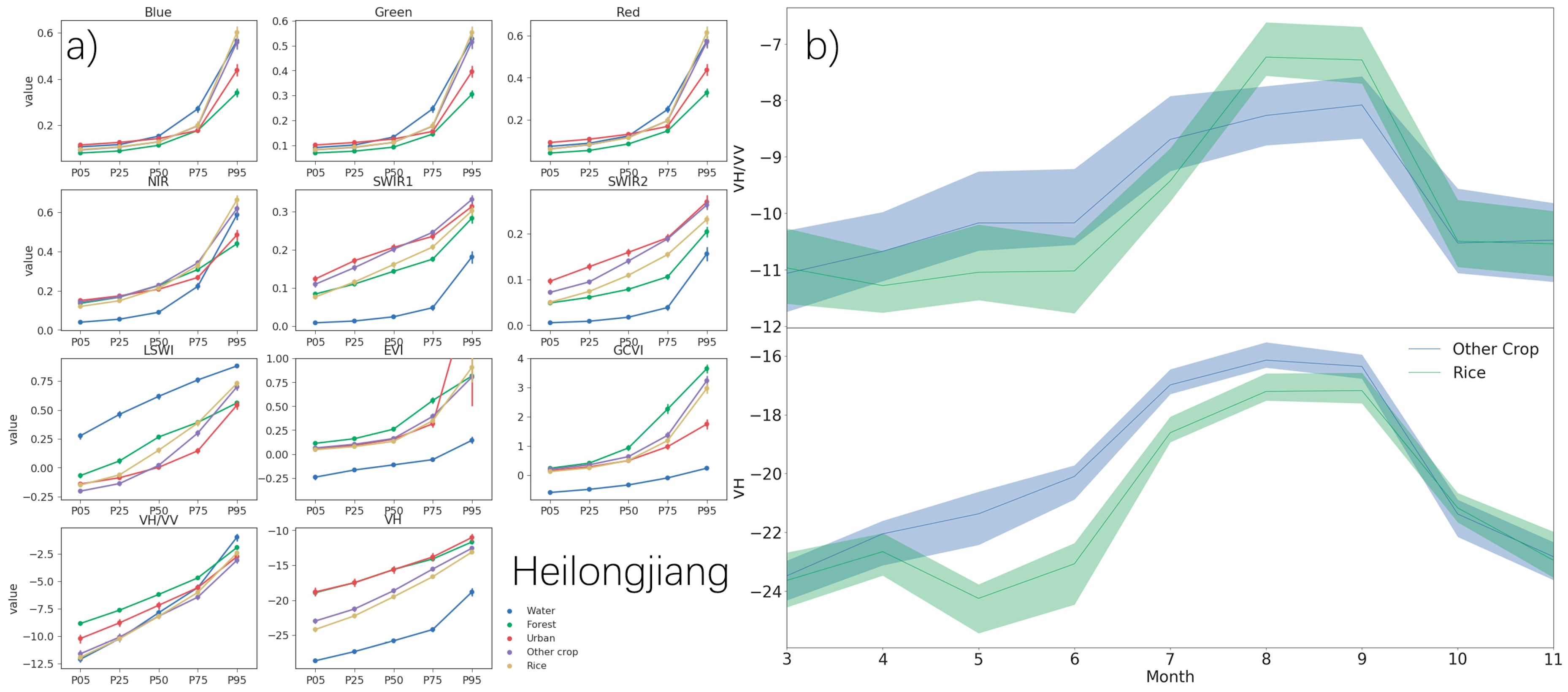
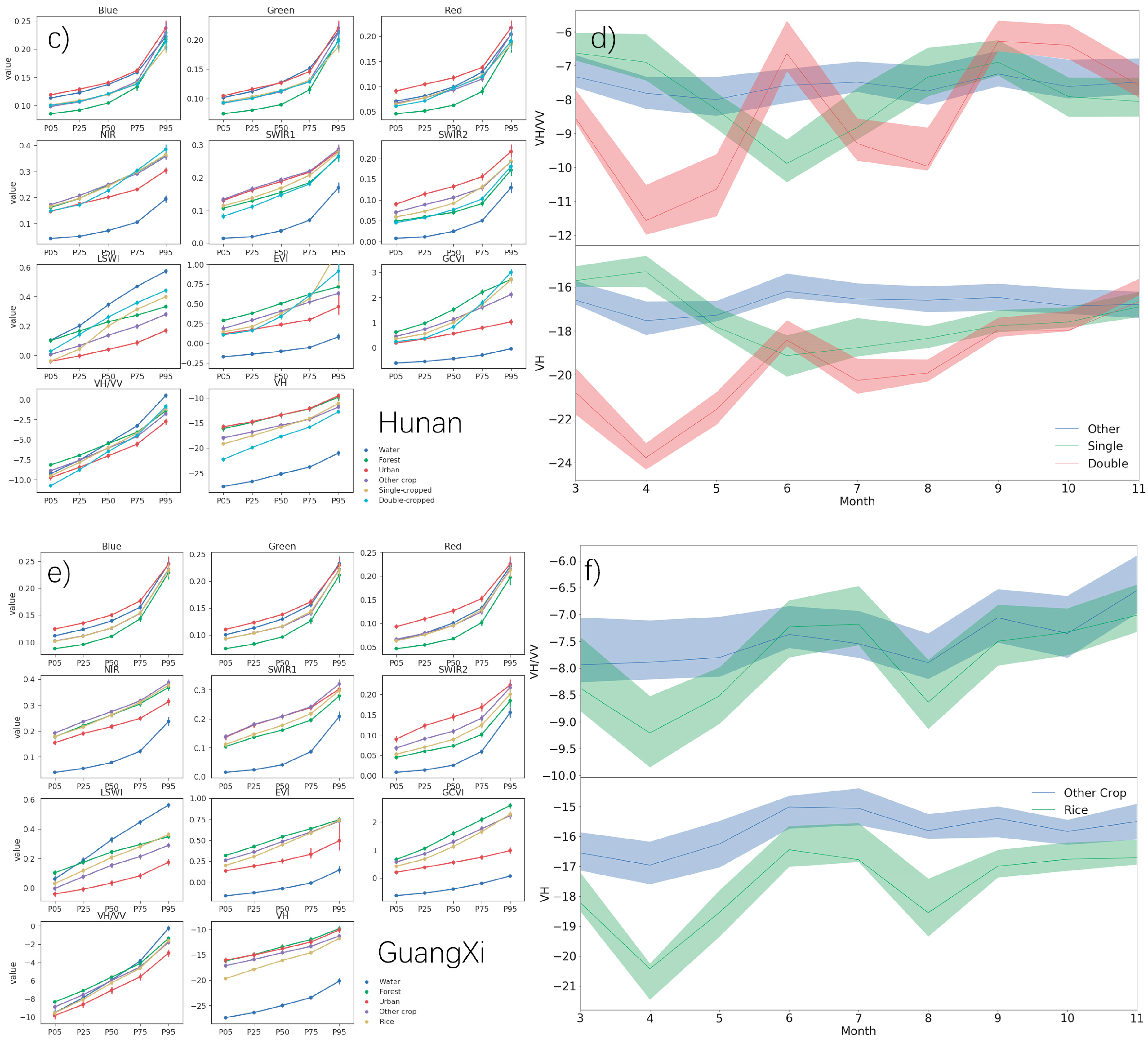
4.1. Monthly and Metric Composites for Each Province
4.2. Accuracy Assessment
5. Discussion
6. Conclusions
Author Contributions
Funding
Acknowledgments
Conflicts of Interest
References
- Kuenzer, C.; Knauer, K. Remote sensing of rice crop areas. Int. J. Remote Sens. 2013, 34, 2101–2139. [Google Scholar] [CrossRef]
- Elert, E. Rice by the numbers: A good grain. Nature 2014, 514, S50. [Google Scholar] [CrossRef] [PubMed]
- Xu, C.C.; Sun, L.J.; Zhou, X.Y.; Li, F.B.; Fang, F.P. Characteristics of Rice Production in South China and Policy Proposals for Its Steady Development. Res. Agric. Mod. 2013, 2, 001. [Google Scholar]
- Frolking, S.; Yeluripati, J.B.; Douglas, E. New district-level maps of rice cropping in India: A foundation for scientific input into policy assessment. Field Crop. Res. 2006, 98, 164–177. [Google Scholar] [CrossRef]
- Bouman, B. How much water does rice use? Management 2009, 69, 115–133. [Google Scholar]
- Tao, F.L.; Hayashi, Y.; Zhang, Z.; Sakamoto, T.; Yokozawa, M. Global warming, rice production, and water use in China: Developing a probabilistic assessment. Agric. For. Meteorol. 2008, 148, 94–110. [Google Scholar] [CrossRef]
- Khush, G.S. What it will take to feed 5.0 billion rice consumers in 2030. Plant Mol. Biol. 2005, 59, 1–6. [Google Scholar] [CrossRef] [PubMed]
- AMIS. AMIS Market Database. 2017. Available online: http://www.gmswga.org/document/amis-market-database (accessed on 27 July 2018).
- Islam, M.S.; Grönlund, Å. Agriculture Market Information Services (AMIS) in the Least Developed Countries (LDCs): Nature, Scopes, and Challenges; Springer: Berlin/Heidelberg, Germany, 2010; pp. 68–70. [Google Scholar]
- Maclean, J.L. Rice Almanac: Source Book for the Most Important Economic Activity on Earth; International Rice Research Institute (IRRI): Los Baños, Philippines, 2002. [Google Scholar]
- Zhang, Q.; Zhang, W.; Li, T.; Sun, W.; Yu, Y.; Wang, G. Projective analysis of staple food crop productivity in adaptation to future climate change in China. Int. J. Biometeorol. 2017, 61, 1445–1460. [Google Scholar] [CrossRef] [PubMed]
- Dong, J.; Xiao, X.; Menarguez, M.A.; Zhang, G.; Qin, Y.; Thau, D.; Biradar, C.; Moore, B., III. Mapping paddy rice planting area in northeastern Asia with Landsat 8 images, phenology-based algorithm and Google Earth Engine. Remote Sens. Environ. 2016, 185, 142–154. [Google Scholar] [CrossRef] [PubMed] [Green Version]
- Gong, P.; Wang, J.; Yu, L.; Zhao, Y.; Zhao, Y.; Liang, L.; Niu, Z.; Huang, X.; Fu, H.; Liu, S. Finer resolution observation and monitoring of global land cover: first mapping results with Landsat TM and ETM+ data. Int. J. Remote Sens. 2013, 34, 2607–2654. [Google Scholar] [CrossRef]
- Mora, B.; Tsendbazar, N.E.; Herold, M.; Arino, O. Global Land Cover Mapping: Current Status and Future Trends; Springer: Dordrecht, The Netherlands, 2014; pp. 250–261. [Google Scholar]
- Dong, J.; Xiao, X. Evolution of regional to global paddy rice mapping methods: A review. ISPRS J. Photogramm. Remote Sens. 2016, 119, 214–227. [Google Scholar] [CrossRef]
- Nguyen, D.B.; Wagner, W. European Rice Cropland Mapping with Sentinel-1 Data: The Mediterranean Region Case Study. Water 2017, 9, 392. [Google Scholar] [CrossRef]
- Torbick, N.; Chowdhury, D.; Salas, W.; Qi, J. Monitoring Rice Agriculture across Myanmar Using Time Series Sentinel-1 Assisted by Landsat-8 and PALSAR-2. Remote Sens. 2017, 9, 119. [Google Scholar] [CrossRef]
- Xiao, X.; Boles, S.; Frolking, S.; Salas, W.; Moore Iii, B.; Li, C.; He, L.; Zhao, R. Observation of flooding and rice transplanting of paddy rice fields at the site to landscape scales in China using VEGETATION sensor data. Int. J. Remote Sens. 2002, 23, 3009–3022. [Google Scholar] [CrossRef]
- Huete, A.; Didan, K.; Miura, T.; Rodriguez, E.P.; Gao, X.; Ferreira, L.G. Overview of the radiometric and biophysical performance of the MODIS vegetation indices. Remote Sens. Environ. 2002, 83, 195–213. [Google Scholar] [CrossRef]
- Gao, B. NDWI—A normalized difference water index for remote sensing of vegetation liquid water from space. Remote Sens. Environ. 1996, 58, 257–266. [Google Scholar] [CrossRef]
- Ramankutty, N.; Foley, J.A. Characterizing patterns of global land use: An analysis of global croplands data. Glob. Biogeochem. Cycles 1998, 12, 667–685. [Google Scholar] [CrossRef] [Green Version]
- Ramankutty, N.; Foley, J.A. Estimating historical changes in global land cover: Croplands from 1700 to 1992. Glob. Biogeochem. Cycles 1999, 13, 997–1027. [Google Scholar] [CrossRef] [Green Version]
- Li, P.; Feng, Z.; Jiang, L.; Liu, Y.; Xiao, X. Changes in rice cropping systems in the Poyang Lake Region, China during 2004–2010. J. Geog. Sci. 2012, 22, 653–668. [Google Scholar] [CrossRef] [Green Version]
- Roumenina, E.; Atzberger, C.; Vassilev, V.; Dimitrov, P.; Kamenova, I.; Banov, M.; Filchev, L.; Jelev, G. Single- and Multi-Date Crop Identification Using PROBA-V 100 and 300 m S1 Products on Zlatia Test Site, Bulgaria. Remote Sens. 2015, 7, 13843–13862. [Google Scholar] [CrossRef] [Green Version]
- Thenkabail, P.S. Mapping rice areas of South Asia using MODIS multitemporal data. J. Appl. Remote Sens. 2011, 5, 863–871. [Google Scholar]
- Zhong, L.; Gong, P.; Biging, G.S. Efficient corn and soybean mapping with temporal extendability: A multi-year experiment using Landsat imagery. Remote Sens. Environ. 2014, 140, 1–13. [Google Scholar] [CrossRef]
- Sakamoto, T.; Yokozawa, M.; Toritani, H.; Shibayama, M.; Ishitsuka, N.; Ohno, H. A crop phenology detection method using time-series MODIS data. Remote Sens. Environ. 2005, 96, 366–374. [Google Scholar] [CrossRef]
- Chen, C.F.; Huang, S.W.; Son, N.T.; Chang, L.Y. Mapping double-cropped irrigated rice fields in Taiwan using time-series Satellite Pour I’Observation de la Terre data. J. Appl. Remote Sens. 2011, 5, 3528. [Google Scholar] [CrossRef]
- Clauss, K.; Yan, H.; Kuenzer, C. Mapping paddy rice in China in 2002, 2005, 2010 and 2014 with MODIS time series. Remote Sens. 2016, 8, 434. [Google Scholar] [CrossRef]
- Zhong, L.; Hawkins, T.; Biging, G.; Gong, P. A phenology-based approach to map crop types in the San Joaquin Valley, California. Int. J. Remote Sens. 2011, 32, 7777–7804. [Google Scholar] [CrossRef]
- Michishita, R.; Jin, Z.; Chen, J.; Xu, B. Empirical comparison of noise reduction techniques for NDVI time-series based on a new measure. ISPRS J. Photogramm. Remote Sens. 2014, 91, 17–28. [Google Scholar] [CrossRef]
- Zhang, X.; Zhang, M.; Zheng, Y.; Wu, B. Crop Mapping Using PROBA-V Time Series Data at the Yucheng and Hongxing Farm in China. Remote Sens. 2016, 8, 915. [Google Scholar] [CrossRef]
- Choudhury, I.; Chakraborty, M. SAR signature investigation of rice crop using RADARSAT data. Int. J. Remote Sens. 2006, 27, 519–534. [Google Scholar] [CrossRef]
- Kurosu, T.; Fujita, M.; Chiba, K. Monitoring of rice crop growth from space using the ERS-1 C-band SAR. IEEE Trans. Geosci. Remote Sens. 1995, 33, 1092–1096. [Google Scholar] [CrossRef]
- Bouvet, A.; Toan, T.L.; Nguyen, L.D. Monitoring of the rice cropping system in the Mekong Delta using ENVISAT/ASAR dual polarization data. IEEE Trans. Geosci. Remote Sens. 2009, 47, 517–526. [Google Scholar] [CrossRef] [Green Version]
- Lam-Dao, N. Rice Crop Monitoring Using New Generation Synthetic Aperture Radar (SAR) Imagery. Ph.D. Thesis, University of Southern Queensland, Toowoomba, Australia, 2009. [Google Scholar]
- Chen, J.; Lin, H.; Pei, Z. Application of ENVISAT ASAR Data in Mapping Rice Crop Growth in Southern China. IEEE Geosci. Remote Sens. Lett. 2007, 4, 431–435. [Google Scholar] [CrossRef]
- Panigrahy, S.; Jain, V.; Patnaik, C.; Parihar, J.S. Identification of Aman Rice Crop in Bangladesh Using Temporal C-Band SAR—A Feasibility Study. J. Indian Soc. Remote Sens. 2012, 40, 599–606. [Google Scholar] [CrossRef]
- Prucker, S.; Meier, W.; Stricker, W. Evaluation of RADARSAT Standard Beam data for identification of potato and rice crops in India. ISPRS J. Photogramm. Remote Sens. 1999, 54, 254–262. [Google Scholar]
- Veloso, A.; Mermoz, S.; Bouvet, A.; Le Toan, T.; Planells, M.; Dejoux, J.F.; Ceschia, E. Understanding the temporal behavior of crops using Sentinel-1 and Sentinel-2-like data for agricultural applications. Remote Sens. Environ. 2017, 199, 415–426. [Google Scholar] [CrossRef]
- Li, J.; Roy, D.P. A Global Analysis of Sentinel-2A, Sentinel-2B and Landsat-8 Data Revisit Intervals and Implications for Terrestrial Monitoring. Remote Sens. 2017, 9, 902. [Google Scholar] [Green Version]
- Vermote, E.; Claverie, M.; Masek, J.G.; Becker-Reshef, I.; Justice, C.O. A Merged Surface Reflectance Product from the Landsat and Sentinel-2 Missions; American Geophysical Union: Washington, DC, USA, 2013. [Google Scholar]
- Claverie, M.; Masek, J.G.; Ju, J. Harmonized Landsat-8 Sentinel-2 (HLS) Product User’s Guide; National Aeronautics and Space Administration (NASA): Washington, DC, USA, 2016. [Google Scholar]
- Torres, R.; Snoeij, P.; Geudtner, D.; Bibby, D.; Davidson, M.; Attema, E.; Potin, P.; Rommen, B.; Floury, N.; Brown, M.; et al. GMES Sentinel-1 mission. Remote Sens. Environ. 2012, 120, 9–24. [Google Scholar] [CrossRef]
- Cossu, R.; Petitdidier, M.; Linford, J.; Badoux, V.; Fusco, L.; Gotab, B.; Hluchy, L.; Lecca, G.; Murgia, F.; Plevier, C.; et al. A roadmap for a dedicated Earth Science Grid platform. Earth Sci. Inform. 2010, 3, 135–148. [Google Scholar] [CrossRef] [Green Version]
- Nemani, R.; Votava, P.; Michaelis, A.; Melton, F.; Milesi, C. Collaborative Supercomputing for Global Change Science. Eos Trans. Am. Geophys. Union 2011, 92, 109–110. [Google Scholar] [CrossRef]
- Gorelick, N.; Hancher, M.; Dixon, M.; Ilyushchenko, S.; Thau, D.; Moore, R. Google Earth Engine: Planetary-scale geospatial analysis for everyone. Remote Sens. Environ. 2017, 202, 18–27. [Google Scholar] [CrossRef]
- Hansen, M.C.; Potapov, P.V.; Moore, R.; Hancher, M.; Turubanova, S.A.A.; Tyukavina, A.; Thau, D.; Stehman, S.V.; Goetz, S.J.; Loveland, T.R.; et al. High-resolution global maps of 21st-century forest cover change. Science 2013, 342, 850–853. [Google Scholar] [CrossRef] [PubMed]
- Pekel, J.F.; Cottam, A.; Gorelick, N.; Belward, A.S. High-resolution mapping of global surface water and its long-term changes. Nature 2016, 540, 418. [Google Scholar] [CrossRef] [PubMed]
- Oreopoulos, L.; Wilson, M.J.; Várnai, T. Implementation on Landsat Data of a Simple Cloud-Mask Algorithm Developed for MODIS Land Bands. IEEE Geosci. Remote Sens. Lett. 2011, 8, 597–601. [Google Scholar] [CrossRef] [Green Version]
- ESA, E.S.A. Sentinel-2 User Handbook; European Space Agency (ESA): Paris, France, 2015; p. 64. [Google Scholar]
- Huete, A.R.; Liu, H.Q.; Batchily, K.V.; Van Leeuwen, W.J.D.A. A comparison of vegetation indices over a global set of TM images for EOS-MODIS. Remote Sens. Environ. 1997, 59, 440–451. [Google Scholar] [CrossRef]
- Veci, L. SENTINEL-1 Toolbox: SAR Basics Tutorial; European Aviation Safety Agency: Cologne, Germany, 2016. [Google Scholar]
- Nelson, A.; Setiyono, T.; Rala, A.B.; Quicho, E.D.; Raviz, J.V.; Abonete, P.J.; Maunahan, A.A.; Garcia, C.A.; Bhatti, H.Z.M.; Villano, L.S.; et al. Towards an Operational SAR-Based Rice Monitoring System in Asia: Examples from 13 Demonstration Sites across Asia in the RIICE Project. Remote Sens. 2014, 6, 94–105. [Google Scholar] [CrossRef]
- Benediktsson, J.A.; Swain, P.H.; Ersoy, O.K. Neural Network Approaches Versus Statistical Methods in Classification of Multisource Remote Sensing Data. IEEE Geosci. Remote Sens. Lett. 1990, 28, 540–552. [Google Scholar] [CrossRef]
- Xiao, X.; Boles, S.; Liu, J.; Zhuang, D.; Frolking, S.; Li, C.; Salas, W.; Moore, B., III. Mapping paddy rice agriculture in southern China using multi-temporal MODIS images. Remote Sens. Environ. 2005, 95, 480–492. [Google Scholar] [CrossRef]
- Farr, T.G.; Rosen, P.A.; Caro, E.; Crippen, R.; Duren, R.; Hensley, S.; Kobrick, M.; Paller, M.; Rodriguez, E.; Roth, L.; et al. The Shuttle Radar Topography Mission. Rev. Geophys. 2007, 45, 361. [Google Scholar] [CrossRef]
- Zha, Y.; Gao, J.; Ni, S. Use of normalized difference built-up index in automatically mapping urban areas from TM imagery. Int. J. Remote Sens. 2003, 24, 583–594. [Google Scholar] [CrossRef]
- Xiao, X.; Boles, S.; Frolking, S.; Li, C.; Babu, J.Y.; Salas, W.; Moore, B., III. Mapping paddy rice agriculture in South and Southeast Asia using multi-temporal MODIS images. Remote Sens. Environ. 2006, 100, 95–113. [Google Scholar] [CrossRef]
- Zhang, M. GVG for IOS. 2017. Available online: https://itunes.apple.com/us/app/apple-store/id1244686128?mt=8 (accessed on 27 July 2018).
- Zhang, M. GVG for Android. 2017. Available online: https://play.google.com/store/apps/details?id=com.sysapk.gvg (accessed on 27 July 2018).
- Costa, H.; Caetano, M. Combining per-pixel and object-based classifications for mapping land cover over large areas. Int. J. Remote Sens. 2014, 35, 738–753. [Google Scholar] [CrossRef]
- Myint, S.W.; Gober, P.; Brazel, A.; Grossman-Clarke, S.; Weng, Q. Per-pixel vs. object-based classification of urban land cover extraction using high spatial resolution imagery. Remote Sens. Environ. 2011, 115, 1145–1161. [Google Scholar] [CrossRef]
- Breiman, L. Bagging predictors. Mach. Learn. 1996, 24, 123–140. [Google Scholar] [CrossRef] [Green Version]
- Ho, T.K. The random subspace method for constructing decision forests. IEEE Trans. Pattern Anal. Mach. Intell. 1998, 20, 832–844. [Google Scholar]
- Pelletier, C.; Valero, S.; Inglada, J.; Champion, N.; Dedieu, G. Assessing the robustness of Random Forests to map land cover with high resolution satellite image time series over large areas. Remote Sens. Environ. 2016, 187, 156–168. [Google Scholar] [CrossRef]
- Sharma, R.C.; Tateishi, R.; Hara, K.; Iizuka, K. Production of the Japan 30-m Land Cover Map of 2013–2015 Using a Random Forests-Based Feature Optimization Approach. Remote Sens. 2016, 8, 429. [Google Scholar] [CrossRef]
- Tian, S.; Zhang, X.; Tian, J.; Sun, Q. Random Forest Classification of Wetland Landcovers from Multi-Sensor Data in the Arid Region of Xinjiang, China. Remote Sens. 2016, 8, 954. [Google Scholar] [CrossRef]
- Wessels, K.J.; Van Den Bergh, F.; Roy, D.P.; Salmon, B.P.; Steenkamp, K.C.; MacAlister, B.; Swanepoel, D.; Jewitt, D. Rapid Land Cover Map Updates Using Change Detection and Robust Random Forest Classifiers. Remote Sens. 2016, 8, 888. [Google Scholar] [CrossRef]
- Benz, U.C.; Hofmann, P.; Willhauck, G.; Lingenfelder, I.; Heynen, M. Multi-resolution, object-oriented fuzzy analysis of remote sensing data for GIS-ready information. ISPRS J. Photogramm. Remote Sens. 2004, 58, 239–258. [Google Scholar] [CrossRef] [Green Version]
- Burnett, C.; Blaschke, T. A multi-scale segmentation/object relationship modelling methodology for landscape analysis. Ecol. Model. 2003, 168, 233–249. [Google Scholar] [CrossRef]
- Adams, R.; Bischof, L. Seeded Region Growing. IEEE Trans. Pattern Anal. Mach. Intell. 1994, 16, 641–647. [Google Scholar] [CrossRef]
- Tilton, J.C. Image segmentation by region growing and spectral clustering with a natural convergence criterion. In Proceedings of the IGARSS ’98, 1998 IEEE International Geoscience and Remote Sensing Symposium, Seattle, WA, USA, 6–10 July 1998. [Google Scholar]
- Baatz, M.; Schäpe, A. Multi-resolution Segmentation-an optimization approach for high quality multi-scale image segmentation. In Proceedings of the Beiträge zum AGIT-Symposium; 2000; pp. 12–23. Available online: http://www.ecognition.com/sites/default/files/405_baatz_fp_12.pdf (accessed on 27 July 2018).
- Roerdink, J.B.; Meijster, A. The watershed transform: definitions, algorithms and parallelization strategies. Fundam. Inform. 2000, 41, 187–228. [Google Scholar]
- Achanta, R.; Shaji, A.; Smith, K.; Lucchi, A.; Fua, P.; Süsstrunk, S. SLIC Superpixels Compared to State-of-the-Art Superpixel Methods. IEEE Trans. Pattern Anal. Mach. Intell. 2012, 34, 2274–2282. [Google Scholar] [CrossRef] [PubMed] [Green Version]
- Van Der Walt, S.; Schönberger, J.L.; Nunez-Iglesias, J.; Boulogne, F.; Warner, J.D.; Yager, N.; Gouillart, E.; Yu, T. Scikit-image: image processing in Python. PeerJ 2014, 2, e453. [Google Scholar] [CrossRef] [PubMed]
- Chan, R.H.; Ho, C.W.; Nikolova, M. Salt-and-pepper noise removal by median-type noise detectors and detail-preserving regularization. IEEE Trans. Image Process. 2005, 14, 1479. [Google Scholar] [CrossRef] [PubMed]
- Xiong, J.; Thenkabail, P.S.; Tilton, J.C.; Gumma, M.K.; Teluguntla, P.; Oliphant, A.; Congalton, R.G.; Yadav, K.; Gorelick, N. Nominal 30-m Cropland Extent Map of Continental Africa by Integrating Pixel-Based and Object-Based Algorithms Using Sentinel-2 and Landsat-8 Data on Google Earth Engine. Remote Sens. 2017, 9, 1065. [Google Scholar] [CrossRef]
- Azzari, G.; Lobell, D.B. Landsat-based classification in the cloud: An opportunity for a paradigm shift in land cover monitoring. Remote Sens. Environ. 2017, 202, 64–74. [Google Scholar] [CrossRef]
- Wang, J.; Xiao, X.; Qin, Y.; Dong, J.; Zhang, G.; Kou, W.; Jin, C.; Zhou, Y.; Zhang, Y. Mapping paddy rice planting area in wheat-rice double-cropped areas through integration of Landsat-8 OLI, MODIS, and PALSAR images. Sci. Rep. 2015, 5, 10088. [Google Scholar] [CrossRef] [PubMed]
- Csillik, O. Fast Segmentation and Classification of Very High Resolution Remote Sensing Data Using SLIC Superpixels. Remote Sens. 2017, 9, 243. [Google Scholar] [CrossRef]
- Audebert, N.; Saux, B.L.; Lefèvre, S. Semantic Segmentation of Earth Observation Data Using Multimodal and Multi-scale Deep Networks. In Asian Conference on Computer Vision; Springer: Cham, Switzerland, 2016. [Google Scholar]
- Long, J.; Shelhamer, E.; Darrell, T. Fully convolutional networks for semantic segmentation. In Proceedings of the IEEE Conference on Computer Vision and Pattern Recognition, Boston, MA, USA, 7–12 June 2015. [Google Scholar]
- Kendall, A.; Badrinarayanan, V.; Cipolla, R. Bayesian SegNet: Model Uncertainty in Deep Convolutional Encoder-Decoder Architectures for Scene Understanding. arXiv, 2015; arXiv:1511.02680. [Google Scholar]
- Ronneberger, O.; Fischer, P.; Brox, T. U-Net: Convolutional Networks for Biomedical Image Segmentation. In International Conference on Medical Image Computing and Computer-Assisted Intervention; Springer: Cham, Switzerland, 2015. [Google Scholar]


| Sensors | Band | Use | Wavelength | Res | Provider |
|---|---|---|---|---|---|
| Sentinel-2 MSI | B2 | Blue | 490 µm | 10 m | ESA |
| B3 | Green | 560 µm | 10 m | ||
| B4 | Red | 665 µm | 10 m | ||
| B8 | Near-infrared | 842 µm | 10 m | ||
| B11 | Short-wave infrared 1 | 1610 µm | 20 m | ||
| B12 | Short-wave infrared 2 | 2190 µm | 20 m | ||
| Landsat 8 OLI | B2 | Blue | 0.45–0.51 µm | 30 m | USGS (United States Geological Survey) |
| B3 | Green | 0.53–0.59 µm | 30 m | ||
| B4 | Red | 0.64–0.67 µm | 30 m | ||
| B5 | Near-infrared | 0.85–0.88 µm | 30 m | ||
| B6 | Short-wave infrared 1 | 1.57–1.65 µm | 30 m | ||
| B7 | Short-wave infrared 2 | 2.11–2.29 µm | 30 m | ||
| Sentinel-1 C | VV | Dual-band cross-polarization, vertical transmission/horizontal receiver | 10 m | ESA | |
| VH | 10 m | ||||
| SRTM | Elevation | 30 m | NASA (National Aeronautics and Space Administration)/USGS | ||
| Landsat | Hansen Global Forest Change | 30 m | GEE | ||
| Landsat | JRC Global Surface Water Mapping | 30 m | GEE | ||
| Sensors (1 March to 30 November 2017) | Heilongjiang | Hunan | Guangxi | |
|---|---|---|---|---|
| Landsat 8 OLI | Scenes | 752 | 187 | 209 |
| Footprints | 53 | 21 | 20 | |
| Sentinel-2 MSI | Scenes | 4116 | 1411 | 1580 |
| Footprints | 86 | 41 | 48 | |
| Sentinel-1 C-band | Scenes | 828 | 364 | 340 |
| Mode | Interferometric wide swath (IW) | |||
| Orbit Properties | Descending | Ascending | Ascending | |
| Heilongjiang | Field Data | |||||
| Other Crops | Rice | Total | User Accuracy | |||
| Map Data | Other crops | 870 | 33 | 903 | 96.35% | |
| Rice | 50 | 298 | 348 | 85.63% | ||
| Total | 920 | 331 | 1251 | |||
| Producer Accuracy | 94.57% | 90.03% | ||||
| Overall Accuracy | 93.37% | F score | 87.78% | |||
| Hunan | Field Data | |||||
| Other Crops | Single Rice | Double Rice | Total | User Accuracy | ||
| Map Data | Other crops | 5 | 5 | 0 | 95 | 94.74% |
| Single rice | 130 | 130 | 6 | 139 | 93.53% | |
| Double rice | 15 | 15 | 50 | 69 | 72.46% | |
| Total | 97 | 150 | 56 | 303 | ||
| Producer Accuracy | 92.78% | 86.67% | 89.29% | |||
| Overall Accuracy | 89.11% | F score | Single rice | 89.97% | ||
| Double rice | 80.00% | |||||
| Guangxi | Field Data | |||||
| Other Crops | Rice | Total | User Accuracy | |||
| Map Data | Other crops | 280 | 5 | 285 | 98.25% | |
| Rice | 11 | 60 | 71 | 84.51% | ||
| Total | 920 | 331 | 1251 | |||
| Producer Accuracy | 96.22% | 92.31% | ||||
| Overall Accuracy | 95.51% | F score | 88.24% | |||
© 2018 by the authors. Licensee MDPI, Basel, Switzerland. This article is an open access article distributed under the terms and conditions of the Creative Commons Attribution (CC BY) license (http://creativecommons.org/licenses/by/4.0/).
Share and Cite
Zhang, X.; Wu, B.; Ponce-Campos, G.E.; Zhang, M.; Chang, S.; Tian, F. Mapping up-to-Date Paddy Rice Extent at 10 M Resolution in China through the Integration of Optical and Synthetic Aperture Radar Images. Remote Sens. 2018, 10, 1200. https://0-doi-org.brum.beds.ac.uk/10.3390/rs10081200
Zhang X, Wu B, Ponce-Campos GE, Zhang M, Chang S, Tian F. Mapping up-to-Date Paddy Rice Extent at 10 M Resolution in China through the Integration of Optical and Synthetic Aperture Radar Images. Remote Sensing. 2018; 10(8):1200. https://0-doi-org.brum.beds.ac.uk/10.3390/rs10081200
Chicago/Turabian StyleZhang, Xin, Bingfang Wu, Guillermo E. Ponce-Campos, Miao Zhang, Sheng Chang, and Fuyou Tian. 2018. "Mapping up-to-Date Paddy Rice Extent at 10 M Resolution in China through the Integration of Optical and Synthetic Aperture Radar Images" Remote Sensing 10, no. 8: 1200. https://0-doi-org.brum.beds.ac.uk/10.3390/rs10081200