Detailed Land Cover Mapping from Multitemporal Landsat-8 Data of Different Cloud Cover

Abstract

Detailed, accurate and frequent land cover mapping is a prerequisite for several important geospatial applications and the fulfilment of current sustainable development goals. This paper introduces a methodology for the classification of annual high-resolution satellite data into several detailed land cover classes. In particular, a nomenclature with 27 different classes was introduced based on CORINE Land Cover (CLC) Level-3 categories and further analysing various crop types. Without employing cloud masks and/or interpolation procedures, we formed experimental datasets of Landsat-8 (L8) images with gradually increased cloud cover in order to assess the influence of cloud presence on the reference data and the resulting classification accuracy. The performance of shallow kernel-based and deep patch-based machine learning classification frameworks was evaluated. Quantitatively, the resulting overall accuracy rates differed within a range of less than 3%; however, maps produced based on Support Vector Machines (SVM) were more accurate across class boundaries and the respective framework was less computationally expensive compared to the applied patch-based deep Convolutional Neural Network (CNN). Further experimental results and analysis indicated that employing all multitemporal images with up to 30% cloud cover delivered relatively higher overall accuracy rates as well as the highest per-class accuracy rates. Moreover, by selecting 70% of the top-ranked features after applying a feature selection strategy, slightly higher accuracy rates were achieved. A detailed discussion of the quantitative and qualitative evaluation outcomes further elaborates on the performance of all considered classes and highlights different aspects of their spectral behaviour and separability.

1. Introduction

Land cover is one of the essential terrestrial climate variables [1] and therefore land cover information in terms of regularly updated, detailed and accurate land cover maps arises as a significant input for several scientific communities working on climate change studies, geomorphology, sustainable development and social sciences, natural resources management and agricultural monitoring. At the same time, open data policies in both the USA and EU are delivering an unprecedented volume of satellite imagery data with an increasing level of spatial, spectral and temporal resolution. Currently, the availability of Landsat-8 (L8) and Sentinel-2 data significantly increases the capacity for high-resolution land cover mapping using dense time series while demanding efficient and cost-effective classification methods. Recent research efforts have focused on the use of finer resolution satellite imagery for land cover map production, offering products at a global scale such as the updated version of FROM-GLC [2], the FROM-GLC-agg [3] product with nine general land cover classes at 30 m and an estimated accuracy of 65.51%, and the recent GlobeLand 30 product [4], providing land cover information at 30 m with 10 land cover classes. Landsat archive data were also employed for national-level product approaches such as the 30 m map of 16 classes from the USA National Land Cover Database [5] as well as the recent land cover map of France with 17 classes and an achieved accuracy of over 80% [6]. Additionally, focusing on agricultural landscapes, Xiong et al. [7] produced a nominal 30-m cropland extent product of the entire African continent using Sentinel-2 and L8 time series for the year 2015, resulting in a weighted overall accuracy of 94.5% for binary classification of cropland versus non-cropland areas.

Beyond the achieved and reported overall accuracy rates, a key aspect of the produced map, in terms of usability and applicability, is the number of land cover classes considered. Most of the aforementioned products do not incorporate a highly analytic classification system and nomenclature in order to deliver detailed information regarding several different land cover classes. On the other hand, mapping products that deliver a rich class nomenclature, like the CORINE Land Cover (CLC), are not regularly updated since they are based mainly on laborious image interpretation and manual digitization procedures. Furthermore, regarding the challenging case of agriculture, even in the detailed CLC product, crop areas like arable land are mapped depicting the implied agricultural practice and not the specific crop cultivated. Recent studies [8,9,10,11] have indicated that crop mapping is quite a challenging problem requiring high spatial and temporal resolution data but also a significant amount of crop-type reference data.

Regarding the production of annual land cover maps based on multitemporal datasets, a number of approaches have employed data from two different seasons [12,13], while the general trend is to employ frameworks that can exploit all the available annual data (below a given cloud presence threshold). However, how and to what extent the presence of clouds affects the accuracy and effectiveness of mapping and monitoring applications has not been studied adequately, and further insights are required [14]. In particular, for discriminating between different crop types, more multitemporal observations are required in order to note key periodic events in the life cycle of different species (phenology), sufficiently capturing spatial, spectral and temporal features [9,10,15]. However, in most geographical regions and climate zones it is rare to find several absolutely clean, cloud-free images [14,16]. The norm is that even the clearest images of a Landsat path/row or Sentinel tile will contain a number of pixels that are affected by different type of clouds. Although, recent efforts are employing cloud masks and interpolation procedures to tackle invalid values and produce synthesized data [6,8,9], cloud detection approaches (e.g., f-mask) fail to detect all clouds/cloud types in a scene (especially cirrus, warm or thin clouds) and therefore even with cloud masks multitemporal datasets include noisy pixels (e.g., clouds, shadows). Moreover, all additional processes (e.g., interpolation) require/cost a significant amount of CPU and/or GPU hours.

Another critical issue concerning land cover map production is the selection of the classification method and algorithm. Supervised classification methods are considered superior to unsupervised for this type of study [6,17,18], but they require the use of accurate and sufficient training data. Additionally, the use of machine learning techniques like Support Vector Machines—SVM [19,20], Random Forests—RF [21] and artificial Neural Networks—NN have gained rapid recognition for classification studies. SVM have been widely used in recent land cover and crop type classification literature [22,23,24,25,26], while in many cases they have been reported to outperform algorithms like RF and NN [18,27,28]. SVM offers the ability to attain high classification accuracies even if using small training sets [27,29,30], and has also proven robust for low noise levels in the presence of mislabelled training data [22]. An important advantage of the SVM classifier is its ability to manage well a large feature space, which is the case when classifying multi-temporal multispectral imagery [31]. RF classifiers have been also reported to achieve high accuracy metrics in similar classification tasks [9,22,32], while studies have indicated that RF may present lower sensitivity to mislabelled training data than SVM [22]. On the other hand, deep learning is currently one of the fastest-growing trends in remote sensing data analysis, successfully tackling a variety of challenging problems and benchmark datasets in object recognition, semantic segmentation and image classification [33,34,35,36]. In particular, Convolutional Neural Networks (CNNs) are currently heavily used for classification and semantic segmentation tasks in a variety of remote sensing datasets [28,37,38,39]. However, compared to more shallow architectures (e.g., SVM), the operational and complexity aspects of CNN-based techniques are directly associated with the considered data dimensionality, which is a key limitation when employing several spectral bands and/or multitemporal datasets [25,40].

Towards addressing the aforementioned challenges, in this paper we introduce a framework for systematic, detailed land cover mapping from annual L8 satellite data. In particular, we consider 27 classes based on CLC Level-3 nomenclature, focusing on the cover type and not the use type classes, while analysing further the crop type classes. Without employing cloud masks or interpolation procedures to recover cloudy pixels, we form different spatio–spectro–temporal datacubes composed of images with gradually increasing levels of cloud cover. Two types of machine learning classifiers, i.e., one with a shallow (SVM) and one with a deep architecture (CNN) were applied and compared. An assessment of the impact on classification accuracy and the robustness of the classifier was performed by classifying the different datacubes. The influence of clouds on the reference data was also evaluated by comparing cloud cover percentages and resulting per-class accuracy. Different sets of classification features were tested by applying a standard feature selection strategy. A detailed analysis and discussion of the validation results is also provided in the last section.

2. Materials and Methods

2.1. Study Area

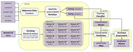
The study area is located in northern Greece and includes the greatest part of Central Macedonia Region, the east part of West Macedonia Region, the northern part of Thessaly Region and also a small area belonging to the former Yugoslav Republic of Macedonia-FYROM (Figure 1, left). It covers an area of about 22,000 km² without including the marine region of the Aegean Sea in the southeast. We selected this region as the study area since it presents highly heterogeneous landscapes, significant land cover diversity including metropolitan centres, vast agricultural areas, high-altitude mountains and water bodies as well as different climate zones, i.e., from sea level to almost 3000 m altitude. Generally, the climate of the region is characterized by rainy winters and dry, warm to hot summers, according to the Köppen climate classification [41,42]. Terrain relief in the whole scene varies greatly, including plains but also several mountain masses scattered across the region such as Mount Olympus, the highest in the country at 2917 m above sea level, the Voras Mountains at 2524 m and the Pierian Mountains at 2190 m.

The main land cover types are natural vegetation and agriculture. Uplands and mountainous areas are covered mainly by broadleaved forests and to a smaller extent by coniferous forests. Lowlands are occupied mostly by Mediterranean-type evergreen sclerophyllous vegetation of bushes, scrubs and maquis. Agricultural land consists principally of permanent crops like vineyards, olive groves and fruit trees (e.g., citrus, apricot, pear, quince, cherry, apple, nut trees). The latter are mainly cultivated in plains around Edessa, Naoussa and Veria. Rice cultivation is also practiced around the Axios River and Aliakmonas River deltas in Central Macedonia. Arable land includes mainly cereals (e.g., wheat, barley, rye, triticale), maize and grass fodder (e.g., clover, alfalfa) fields. Artificial land is typically comprised of cities and towns, including the metropolitan area of Thessaloniki, the second-largest city in Greece. Smaller towns and villages are scattered across the region. In addition, major water bodies of the country are situated in our study area such as Volvi and Koroneia Lakes and Haliacmon, Axios and Strymonas Rivers in Central Macedonia and also Vegoritida and Polyfytos Lakes in West Macedonia. Low-lying marches land, usually flooded, can be found near water bodies but also on river estuaries to the Aegean Sea.

2.2. Landsat-8 Annual Datasets

All surface reflectance L8 products for the 182/34 path/row of the year 2016 were downloaded from the USGS (United States Geological Survey) EarthExplorer platform. The L8 Surface Reflectance product is generated at 30-m spatial resolution on a Universal Transverse Mercator (UTM) projection including seven multispectral bands from the Ultra Blue to the Shortwave Infrared (SWIR) spectral regions. Based on our previous research efforts [43,44], we selected all annual data with less than 60% of cloud cover (over the land) for the experiments. In order to address our main goal for assessing the impact of integrating images with gradually increased cloud cover, four different datasets were formed including images with: #1. Less than 20% (11 dates); #2. Less than 30% (14 dates); #3. Less than 40% (16 dates) and #4. Less than 60% (18 dates) land cloud cover. Moreover, a smaller dataset formed with six images (Dataset #0) of approximately less than 10% land cloud cover was used for the comparison between the two different classification architectures (see Section 3.1). It is important to mention that all datasets include dates from all four seasons and not just summer or spring (

Table 1. Land cloud cover (LCC), acquisition dates and the corresponding season are presented for each image along with the LCC limit.

Image #	LCC	Date of Acquisition	Season	LCC Limit	# of Dataset
1	1.19%	8/1/2016 *	Winter	<20%	1	2	3	4
2	15.23%	24/1/2016	Winter
3	10.24%	13/4/2016 *	Spring
4	0.05%	31/5/2016 *	Spring
5	0.19%	16/6/2016 *	Summer
6	10.86%	2/7/2016 *	Summer
7	12.99%	18/7/2016	Summer
8	11.46%	19/8/2016	Summer
9	12.36%	4/9/2016	Autumn
10	12.03%	20/9/2016	Autumn
11	0.73%	9/12/2016 *	Winter
12	27.11%	28/3/2016	Spring	<30%
13	24.14%	3/8/2016	Summer
14	26.92%	6/10/2016	Autumn
15	37.06%	9/2/2016	Winter	<40%
16	31.94%	15/5/2016	Spring
17	46.66%	7/11/2016	Autumn	<60%
18	58.79%	25/12/2016	Winter

* Corresponds to images of Dataset #0 with ~10% LCC limit.

).

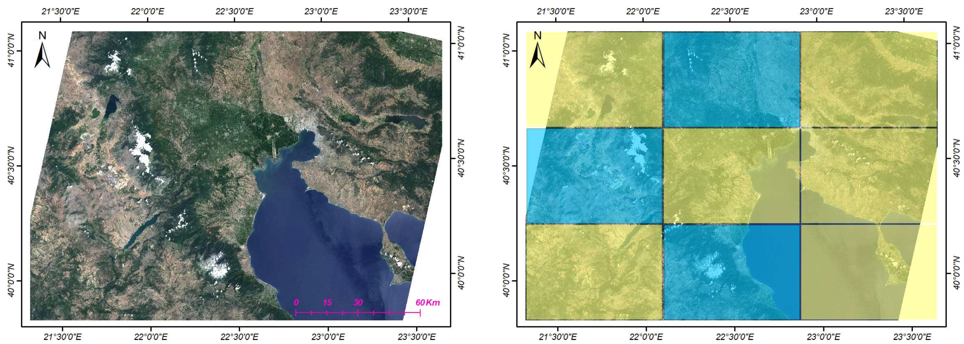
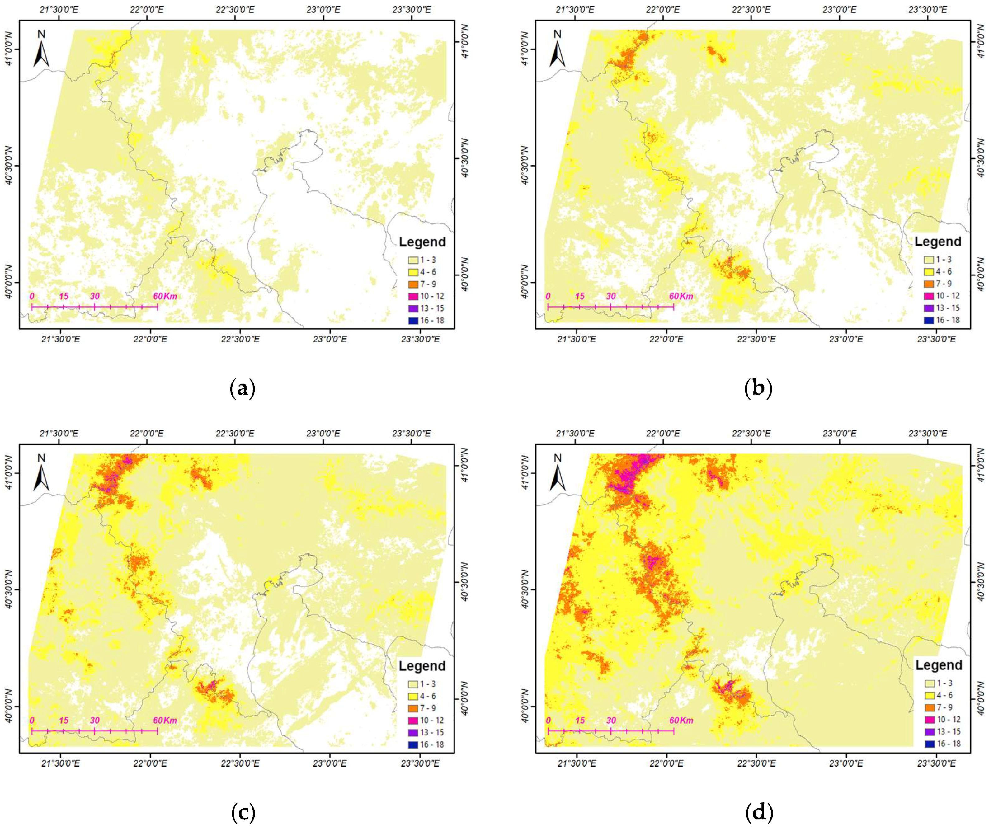
In Figure 2, cumulative cloud maps are presented, indicating per pixel the frequency of cloud cover per dataset in the study area. The cloud presence per-image was derived from the F-mask algorithm [45] and the Quality Assessment (QA) L8 band. In particular, for the first dataset (Dataset #1), a large continental part of the study area is cloud-free (white) across the corresponding 11 dates/images. Moreover, pixels that are occasionally covered by clouds mainly have a cloud frequency of up to three dates (beige). Regarding Dataset #2 (14 images in total), a large part of the study area is covered in cloud for up to three out of 14 dates. However, there are parts that are reported with up to six (and even up to nine) cloudy dates, mainly from northwest to south following the mountain massifs formations of the study area. This is also the case and in a more intense frequency for Dataset #3 (16 dates), where generally the regions that had up to three dates frequency in Dataset #1 are reported in #3 with a frequency of up to six cloudy dates. The most cloudy Dataset #4 (18 dates) is mostly covered at three to six dates, while certain mainly mountainous regions are covered by cloud for up to 12 dates (magenta) and up to 15 dates (purple) out of the 18 dates/images of the dataset.

2.3. Land Cover Classes and Reference Data

One of the main contributions of this paper is that the proposed methodology has been designed, developed and validated for a detailed land cover classification into more than 25 land cover classes. In particular, the developed nomenclature was mainly derived from the CLC nomenclature [46] while the main crop types were based on the available geospatial data of the Greek Payment Authority of the Common Agricultural Policy (CAP). The introduced land cover class nomenclature for this study was formed starting from the CLC2012 Level-3 subclasses and by either grouping, i.e., merging classes (e.g., 4.1.1 Inland and 4.2.1 Salt marches) or splitting further classes (e.g., Dense and Sparse 3.2.3 Sclerophyllous vegetation) when needed.

Additionally, certain exclusions or modifications were applied mainly with the use type classes (e.g., 1.4.2 Sport and leisure facilities), with classes that were not present in our study area (e.g., 3.3.5 Glaciers and perpetual snow) and also with classes that are defined for the CLC-specific scale (e.g., 2.4.2 Complex cultivation patterns), since CLC uses a minimum mapping unit of 25 hectares. Agriculture classes were further analysed based on available geospatial data. The introduced nomenclature, including 27 different classes, is presented in

Table 2. The detailed land cover nomenclature with 27 classes. The number of available polygons and pixels used for training and testing are presented for every class.

Land Cover Nomenclature	Code	Description	Pol.	Tr. Pixels	Test Pixels
1. Dense Urban Fabric	DUF	Land covered by structures in a continuous dense fabric—big cities.	126	3452	1332
2. Sparse Urban Fabric	SUF	Land covered by structures in a discontinuous sparse fabric	270	2608	1739
3. Industrial Commercial Units	ICU	Artificially surfaced industrial or commercial units.	128	1046	697
4. Road/Asphalt Networks	RAN	Asphalt sealed areas and networks.	79	558	183
5. Mineral Extraction Sites	MES	Areas with open-pit-extraction of construction material or minerals.	36	1898	1265
6. Broad-leaved Forest	BLF	Forest with broad-leaved species predomination.	1359	15,000	10,000
7. Coniferous Forest	CNF	Forest with coniferous species predomination.	938	5737	3825
8. Natural Grasslands	NGR	Areas of herbaceous vegetation.	265	445	297
9. Dense Sclerophyllous Vegetation	DSV	Dense bushy sclerophyllous vegetation, including maquis and garrigue.	502	4058	2075
10. Sparse Sclerophyllous Vegetation	SSV	Sparse bushy sclerophyllous vegetation, including maquis and garrigue.	396	5056	1233
11. Moss and Lichen	MNL	High altitude moors areas with moss and lichen.	154	1046	295
12. Sparsely Vegetated Areas	SVA	Scattered vegetation areas on stones, boulders, or rubble on steep slopes.	65	767	511
13. Vineyards	VNY	Areas of vine cultivation.	269	836	557
14. Olive Groves	OLG	Areas of olive trees plantations.	517	1048	262
15. Fruit Trees	FRT	Areas of fruit trees plantations, including citrus, apricot, pear, quince, cherry, apple and nut trees.	579	973	649
16. Kiwi Plants	KWP	Areas of kiwi plants cultivation.	172	479	303
17. Cereals	CRL	Areas of cereal crops cultivation, including wheat, barley, rye and triticale.	504	1268	851
18. Maize	MAZ	Areas of maize crop cultivation.	179	351	234
19. Rice Fields	RCF	Areas of rice cultivation—periodically flooded.	999	11,775	6483
20. Potatoes	PTT	Areas of potato cultivation.	78	277	185
21. Grass Fodder	GRF	Areas of grass fodder cultivation, including clover and alfalfa.	500	610	407
22. Greenhouses	GRH	Structures with glass or translucent plastic roof where plants are grown.	96	114	76
23. Rocks and Sand	RNS	Bare land areas consisting of rock, cliffs, beaches and sand.	295	2331	1554
24. Marshes	MRS	Low-lying land usually flooded by water/sea water and partially covered with herbaceous vegetation.	52	7082	1833
25. Water Courses	WCR	Natural or artificial water courses—rivers and canals.	67	776	277
26. Water Bodies	WBD	Natural or artificial stretches of water—lakes.	17	15,000	6567
27. Coastal Water	CWT	Sea water of low depth on coastal areas.	30	3928	982

.

An intensive manual annotation procedure was carried out for the production of reference data. Two image interpretation experts who are also familiar with the CLC product and the study area manually digitized polygons for the different land cover classes. Since representative training samples are one of the most critical components in supervised classification, the experts studied the area thoroughly and intensively and noted as many variations of each class as possible. The annotation of each sample followed the principle of avoiding mixtures of the defined land cover classes [2]. Different data sources and multitemporal images were employed for the photointerpretation and annotation process, including Sentinel 2 and L8 images for the year of 2016, Google Earth Pro data for 2016 using Historical Imagery, the CLC2012 product and available CAP geospatial data for the crop fields of 2016. CAP geospatial data are collected by the agency through field surveys on a yearly basis. In Table 2 one can observe the number of available polygons for each class and the number of pixels used for training and testing for each category, as described in Section 2.4.2.

2.4. Land Cover Mapping Framework

2.4.1. Classification Features

Spectral features, in most cases referring to sensor multispectral bands but also spectral indices, have been widely used as the main set of input features for land cover classification in the recent literature [8,36,47,48,49]. Based on our previous research efforts [43,44] and on the related bibliography, the seven atmospherically corrected L8 spectral bands were used, along with four selected spectral indices generally addressing vegetation, water and man-made regions. More specifically, we used surface reflectance features of bands: Ultra Blue (0.435–0.451 μm), Blue (0.452–0.512 μm), Green (0.533–0.590 μm), Red (0.636–0.673 μm), Near Infrared—NIR (0.851–0.879 μm), Shortwave Infrared—SWIR 1 (1.566–1.651 μm), Shortwave Infrared—SWIR 2 (2.107–2.294 μm), and the Normalized Difference Vegetation Index (NDVI) [50], the Modified Soil-Adjusted Vegetation Index (MSAVI) [51], the Normalized Difference Water Index (NDWI) [52] and the Normalized Difference Built-up Index (NDBI) [53]. These 11 spectral features were stacked together for each date and then four spectral cubes of multiple dates were formed based on different cloud cover levels, as described in Section 2.2.

2.4.2. Training and Testing Areas

Reference data were created through an intensive manual annotation procedure and were divided into two independent sets: one for the training and one for the validation procedure. To avoid any spatial correlation between the training and validation datasets, the study area was partitioned in nine different blocks. Six of them were used for the training procedure and the remaining three for the testing one (Figure 1, right). Strips of 900 m around the borders of the blocks were excluded in order to avoid correlation between the training and validation phases when applying the patch-based deep CNN classification. Regarding the sample size, we applied as minimum reference dataset size required for accuracy assessment, the rule of thumb proposed by [54], whereby 75–100 testing sample units (pixels in our case), per thematic class should be regarded for large areas and complex maps of more than 12 classes [25,55]. Moreover, mainly for computational reasons, the maximum number of pixels per class was limited to 15,000 pixels for training and 10,000 for testing. The pixel’s number limitation was performed with a random selection on the available reference data of each class that exceeded these limits. In addition, another random selection was performed, in order to ensure that the training set, per-class, included a 60% to 80% of all reference pixels and the testing set a 20% to 40%, respectively. This was due to the fact that the annotated polygons did not cover the study in a uniform way.

2.4.3. Experimental Setup

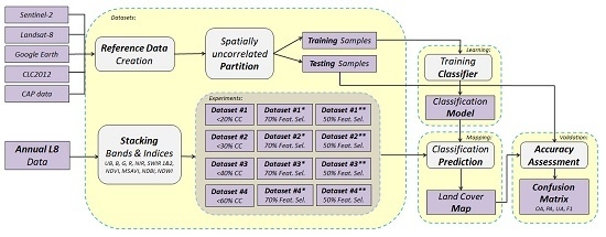
Workflow: First, we ran two comparative experiments, for evaluating the performance of the SVM and CNN frameworks. Due to the high computational power and memory that was required for the CNN implementation, the initial experiments were performed on a spatiotemporal datacube with six dates (Dataset #0) and also on Dataset #1 with 11 dates (Table 1), but using a smaller subset of the reference data (i.e., approximately 30%). Based on the quantitative and qualitative evaluation, the SVM classifier was chosen to be applied for the main four classification experiments towards assessing the impact of integrating images of gradually increased cloud cover in the datasets (Section 3.2). Note, that for these experiments the computational requirements were gradually increased since for the first dataset (Dataset #1, 11 dates), the datacube contained 121 layers/features, for Dataset #2 (14 dates) contained 154, for Dataset #3 (16 dates) 176 and for Dataset #4 (18 dates) contained 198 features. Furthermore, additional experiments were performed by employing a subset of the most significant features for all datasets based on a feature selection strategy (Section 3.3). The pipeline of the developed classification framework and performed experiments are illustrated in the flowchart in Figure 3.

Classification Algorithms: We compared the performance of two classification frameworks that have demonstrated high accuracy rates in the recent literature, i.e., one shallow kernel-based classifier (SVM) and one patch-based deep learning approach (CNN). In particular, a SVM classifier [19,20] from the LIBSVM library using the C-SVC type was employed [56]. For the SVM application different kernel functions have been proposed in the literature [22,57]. In this study, we employ two kernel functions: a linear one that has been proposed and tested as optimal when the number of features is large [58] and has resulted in relatively high accuracy rates in our previous studies [43,44], and the Radial Basis Function (RBF). The tuning of parameter C, referring to the cost of error penalty, is required for both kernels, while the RBF kernel also needs the definition of a second parameter g > 0, which denotes the width of the Gaussian kernel function. For our experiments, the classifiers parameters have been optimized by a five-fold cross validation grid search process: C = {0.01, 0.1, 1, 10, 100, 1000}, g = {0.0001, 0.001, 0.01, 0.1, 1, 10}.

For the deeper architecture among those that have been employed recently for classification tasks [33,34,35,37,59] we employed the relatively simple CNN architecture of the ConvNet Network. The network consists of 10 layers: two convolutional, two max pooling, two batch normalization, two activation functions (rectified linear unit—ReLU) and two fully connected (Figure 4). We used a patch of 29 × 29 pixels centred in the pixel of interest. For the training, we randomly selected patches centred on the training pixels allowing them to overlap. During the validation phase, for each pixel we centred and extracted a patch. Then the predicted label was assigned to this specific pixel. More specifically, the raw input patch for Dataset #1 of 11 dates with size 121 × 29 × 29 is given as input to the first convolutional layer, which applied convolutional kernels of size 5 × 5. Next comes a transfer function layer that applies a ReLU element-wise to the input tensor and is followed by a batch normalization layer. Then a max-pooling layer follows, which downsamples with a size of 2 × 2 the input and lightens the computational burden. The next four layers follow the same pattern, with exactly the same parameters, and result in two final, fully connected layers that produce the final outputs classified in 27 different classes. For Dataset #0 of six dates the architecture remains the same, except for the size of the input patch, which changes to 66 × 29 × 29. The network had been trained using the stochastic gradient descent (SDG) optimizer for 30 epochs and early stopping had been used to prevent overfitting. We set the batch size to 100, the learning rate to 0.1 while every 3 epochs had been reduced by 0.01, the momentum to 0.9 and the weight decay parameter to 5 × 10⁻⁵. For the extraction of the training patches, the only selection criterion was the central pixel of the patch to belong to the specific class. For testing, a patch was extracted in each pixel of the image and the predicted value was assigned to the central pixel.

Feature Selection: In order to further evaluate the contribution of the employed features, a dimensionality reduction procedure was applied in all four datasets. Generally speaking, feature selection methods can be categorized into three types: filter, wrapper, and embedded [60,61]. The filter methods that rank the discriminative power of each feature are independent of the learning process. The other two incorporate the supervised learning algorithm in their approaches for estimating the contribution of each feature. Nonetheless, the last two are also computationally expensive, thereby preventing their use in tasks where the dimensionality and the amount of the data are large [61]. To this end, for our experiments, where the volume of features is large, we selected a computationally efficient filter-based method [62,63], independently of the classification algorithm to be applied. In particular, we employed the Fisher score [60] selection strategy, which calculates the ratio of interclass separation and intraclass variance for each feature and thus expresses the discriminative power of each feature [61,64]. The Fisher score is one of the most widely used supervised feature selection methods and has been combined with SVM classifications in many recent studies [62,65,66,67,68]. In detail, the Fisher score of the rth feature is computed by the formula

$$F_r=\frac{{{\displaystyle \sum }}_{w=1}^c{n}_w{\left({\mu }_w^r-{\mu }_r\right)}^2}{{{\displaystyle \sum }}_{w=1}^c{n}_w{\sigma }_w^r{}^2},$$

(1)

where $n_w$ is the number of samples in class w, ${\mu }_w^r$ and ${\sigma }_w^r$ are the mean and standard deviation of the w-th class for the rth feature, ${\mu }_r$ the mean of the whole data set for the rth feature while the serial number or classes goes from 1 to c. Based on the Fisher score, all features across the temporal cube were ranked and two extra classification experiments for each of the four datasets were performed using the 70% and the 50% of the top ranked features.

Validation Accuracy Metrics: All performed experiments were evaluated qualitatively through a thorough visual inspection as well as quantitatively forming confusion matrices, i.e., double entry tables where row entries are the actual classes corresponding to the testing data and column entries are the predicted classes from the classifier. The standard accuracy metrics of Overall Accuracy (OA), User’s (UA), Producer’s Accuracy (PA) and Kappa coefficient (Kappa) were calculated for each case [69]. Additionally the combined metric of per class F-measure (F1) score is also provided, calculated as the harmonic mean of UA and PA:

$$\mathrm{F}1=\left(2\times \mathrm{UA}\times \mathrm{PA}\right)/\left(\mathrm{UA}+\mathrm{PA}\right).$$

(2)

Additionally, to assess the statistical significance of the accuracy differences between pairs of the different classification algorithms, we employed the McNemar test, since we have used identical testing sets (related samples) for the accuracy assessment [25,70].

3. Experimental Results and Discussion

In this section, experimental results are presented regarding the performance of the classification algorithms (Section 3.1), the influence of the different cloud cover conditions (Section 3.2) on accuracy metrics, the importance of the number and type of features (Section 3.3 and Section 3.4 ), as well as the per-class performance analysis and overall quantitative and qualitative evaluation of the mapping (Section 3.5).

3.1. Comparing the Performance of the SVM and CNN Frameworks

The initial comparative experiments, for evaluating the performance of the SVM with linear and RBF kernels and the CNN framework, were performed on Dataset #0 and Dataset #1 (Section 2.2). Both training and testing datasets were kept exactly the same for both the SVM and the CNN classification frameworks.

Table 3. Quantitative results after the application of the SVM and CNN classifiers.

Dataset	Classifier	Average			OA	Kappa
		PA	UA	F1
Dataset #0 (6 dates)	SVM-linear, C = 100	68.28%	68.74%	66.20%	68.71%	67.25%
	SVM-RBF, C = 10, g = 1	67.63%	69.50%	66.29%	67.36%	65.83%
	CNN	63.36%	64.55%	61.67%	67.23%	65.69%
Dataset #1 (11 dates)	SVM-linear, C = 10	69.01%	69.67%	67.04%	68.66%	67.21%
	SVM-RBF, C = 1000, g = 0.01	67.71%	67.91%	65.18%	67.18%	65.67%
	CNN	63.61%	66.09%	62.64%	69.35%	67.91%

summarizes the resulting quantitative results for all classifiers regarding the average PA, UA and F1 metrics as well as the OA and Kappa accuracy metrics. For all experiments, the OA and Kappa differ with less than 2.3%. Regarding the per-class accuracy metrics, the average PA, UA and calculated F1 metrics highlighted that the SVM classifier with both kernel choices reported higher accuracy rates (up to 5.4%) when comparing with the CNN results. Overall, the linear SVM scored the highest rates for the majority of validation metrics on both datasets.

In order to objectively assess the aforementioned differences, the McNemar test was employed [70]. In particular, the conventional threshold for declaring statistical significance of 5% was adopted, i.e., a p-value of less than 0.05 declares significance.

Table 4. Statistical significance of the compared classification frameworks.

Dataset	Fr. #1	Fr.#2	p-Value	Statistical Significance
Dataset #0 (6 dates)	SVM-linear	SVM-RBF	0.00002	Yes, 0.1%
	SVM-linear	CNN	0.00044	Yes, 0.1%
	SVM-RBF	CNN	0.56414	No, 5%
Dataset #1 (11 dates)	SVM-linear	SVM-RBF	0.00001 × 10−6	Yes, 0.1%
	SVM-linear	CNN	0.01151	Yes, 5%
	SVM-RBF	CNN	0.46276	No, 5%

presents the recorded p-values of the McNemar test for all combinations of the two experiments performed, along with the level of significance stated for significant differences. Apart from the SVM-RBF with CNN pair on both datasets, all other differences were found to be significant at the 5% level of significance, while differences between different kernel SVM classifiers were also found to be statistically significant for the stricter 0.1% level of significance.

Furthermore, in Figure 5 (top) the resulting land cover maps for the CNN and linear SVM are presented. Their disagreement (in black) can be also observed (Figure 5, bottom) as well as the reference data for this particular region. After a closer look, one can observe that the resulting land cover map from the CNN, due to its patch-based nature, tends to generalize the prediction, especially across the class boundaries. Consequently, it resulted in a coarse generalized output including certain omission cases especially for linear objects like roads and rivers as well as for regions with high heterogeneity (e.g., small parcels of different crop type). Regarding the spatial distribution of the differences (Figure 5, bottom left), they are scattered in the entire region mainly across class boundaries, apparently due to the generalized CNN output effect. In particular, these observations are obvious in areas of heterogeneous texture like mixed agricultural areas and other natural areas with frequent cover variation. On the other hand, large areas with continuous single-class coverage, e.g., sea, rice fields and urban regions, present less disagreement between the two land cover products. In comparison with the reference data (Figure 5, bottom right), both resulting maps present relatively high agreement in most cases.

In overall, SVM delivered higher reliability and accuracy for individual classes and more crisp and accurate boundaries. Taking also into consideration the high computational cost of the CNN framework, we chose to perform the main experiments for assessing the impact of different cloud conditions and number of features based on the linear SVM classification framework.

3.2. Assessing the Influence of Different Cloud Cover Conditions

In order to assess the influence of cloud cover conditions in classification, we performed several experiments on the four datasets (Table 1), which were formed by adding more images with incrementally increasing cloud cover over the land. In all experiments the same training and testing sets were employed. For the linear SVM, the C parameter value was set to 0.1. The main question here was whether the addition of more dates/features would help the classifier by adding more observations and potentially strengthening certain phenological characteristics, especially for crop type discrimination, or impede performance by deteriorating class statistics due to the increased presence of clouds.

In Figure 6, the resulting accuracy scores after classifying the four different datasets are presented. In all cases the OA and Kappa coefficient indicated a quite good performance, with rates of over 72%. The highest score was achieved for Dataset #1 (with the lower amount of cloud cover, i.e., <20%) with an OA at 80.5% and Kappa at 78.0%. For the second dataset, when adding three more images with up to 30% clouds, the resulting OA and Kappa rates decreased slightly (~1%). By adding more cloudy images (Datasets #3 and #4) the OA and Kappa rates decreased further by approximately 4.5%. Regarding the average PA, UA and F1 scores, the second dataset resulted in slightly higher accuracy rates than the first one, with rates of 69.1%, 67.6% and 66.4%, respectively. By adding more images with higher than 30% cloud cover, the PA, UA and F1 scores dropped below 66%.

Additionally, in Figure 7 (bars) all the resulting per-class F1 scores for all four datasets are presented. After a close look, one can observe that certain classes, e.g., BLF, KWP, CRL, RCF, WBD and CWT, stand out as the most accurately classified, since they achieve F1 scores of over 80% for all datasets. In 13 of 27 cases, the highest F1 rates were achieved for Dataset #2, while Dataset #1 follows, holding the best rate for nine classes. More specifically, natural vegetation classes like CNF, NGR, SSV, SVA and MRS present higher rates for Dataset #2, like most of the agriculture classes (OLG, RCF, PTT, GRF, GRH). Dataset #4 (more images, more clouds) delivered the higher F1 scores for four classes among those three agricultural varying cycle ones, i.e., FRT, KWP and MAZ.

Influence of clouds in the reference data: In order to evaluate the influence of cloud presence in the reference data (training and testing sets) we estimated the cloud masks for all images based on the F-mask algorithm [45] and the QA band. In Figure 7 (lines), the average per-class cloud presence in the reference data for all datasets is presented. As expected, the cloudy pixels in the reference data are increasing from Dataset #1 to #4. The reference data for the PTT class is an exception since Dataset #2 presents a lower proportion of cloudy pixels than Dataset #1, indicating that the three additional images offered a significant amount of non-cloudy observations. Generally, most classes do not exceed the 20% of cloud cover in the reference data.

The highest rates of cloudy pixels in the reference data are recorded for the classes MNL (48.1–55.5%) and SVA (18.7–33.3%), which are usually found in alpine areas of high altitudes. By comparing both lines and bars of Figure 7, one can observe that for most classes that achieved higher scores in Dataset #2 (like DUF, RAN, SSV, OLG, RCF, GRF, GRH, MRS and WCR), the cloud presence in Dataset #2 did not exceed 10% but was slightly higher than in Dataset #1. This fact indicates that the trade-off between more observations, in terms of more images and less reliable observations, i.e., more cloudy pixels, was favourable for these cases. Another interesting point is that most classes (except for KWP) that, as analysed in the previous paragraph, achieved high rates of over 80% for all datasets, were not the ones that reported the lowest presence of clouds in the reference data.

It should also be highlighted that a significant increase in the cloud presence (in the reference data) between the less cloudy dataset and the cloudiest one does not result in an equivalent decrease in the reported accuracy (F1) rates (Figure 7). For example, the land cover classes of ICU and RCF have an almost 20% difference in cloud presence (comparing the 1st and 4th dataset), while the reported F1 scores differ by less than 7%. This is also the case for the largest differences on the reported F1 scores. For example, classes MES and GRH resulted in a 53% (1st–4th datasets) and a 31% (2nd and 3rd datasets) difference in the F1 scores, respectively, while the corresponding differences of cloud presence on the reference data were 13% and 0.1%, respectively.

These observations can be also justified from

Table 5. Highest achieved F1 scores (%) per class, associated with the corresponding dataset and average cloud presence (%) in the reference data.

Class	DUF	SUF	ICU	RAN	MES	BLF	CNF	NGR	DSV	SSV	MNL	SVA	VNY	OLG	FRT	KWP	CRL	MAZ	RCF	PTT	GRF	GRH	RNS	MRS	WCR	WBD	CWT
# Dataset	2	1	1	2	1	1	2	2	4	2	1	2	1	2	4	4	3	4	2	2	2	2	1	2	2	1	1
F1(max.)	73.3	77.5	62.6	65.2	60.5	91.4	76.1	43.3	41.5	52.1	41.9	42.3	73.8	49.9	51.6	91.8	92.8	78.4	99.5	80.1	50.6	70.8	53.9	62.0	76.2	99.6	97.4
Cloudy pixels	8.0	2.3	1.1	6.9	4.7	9.7	14.2	10.5	10.2	9.0	48.1	24.9	2.5	5.2	11.8	3.1	10.3	13.8	7.6	8.3	5.6	3.3	10.1	5.6	7.4	6.8	6.3

, which presents the highest F1 scores per class, the corresponding dataset and the average cloud presence in the reference data of this dataset. In particular, the highest F1 scores (except for KWP) were not achieved from classes with the lowest rates of cloudy pixels (marked with green). Generally, cloud cover of more than 25% (e.g., MNL, SVA) resulted in relatively low accuracy rates. Overall, the combined analysis did not find a direct relationship between cloud presence and F1 scores achieved, indicating that the combination of the spatial, spectral and temporal resolution of the data along with the intrinsic characteristic and phenological behaviour of each class determines how successful the classification will be.

3.3. Assessing the Influence of Feature Selection

In order to assess the impact of dimensionality reduction on the classification accuracy, additional experiments were performed based on the SVM classification framework (Section 2.4.3), applying a feature selection strategy. In particular, classification results derived by employing all available features were compared with the ones derived by using the 70% and the 50% of the top ranked features based on the calculated Fisher score per dataset.

In

Table 6. Validation metrics (%) for experiments performed: PA, UA and F1 rates are presented per class, while their average rates, the OA and the kappa metric are displayed in the last three rows per experiment. Per-class accuracy rates below 40% are coloured red while those over 80% are marked with bold. The overall highest Average (Aver.), OA and Kappa rates (last three rows) are marked bold, while the lowest ones are double underlined.

Dataset		Dataset 1 (11 Dates) < 20% CC									Dataset 2 (14 Dates) < 30% CC									Dataset 3 (16 Dates) < 40% CC									Dataset 4 (18 Dates) < 60% CC
		All 121 Features			Top 70% 85 Features			Top 50% 60 Features			All 154 Features			Top 70% 107 Features			Top 50% 77 Features			All 176 Features			Top 70% 123 Features			Top 50% 88 Features—15 Dates *			All 198 Features			Top 70% 138 Features			Top 50% 99 Features—16 Dates **
Class	Train. Pixels	PA	UA	F1	PA	UA	F1	PA	UA	F1	PA	UA	F1	PA	UA	F1	PA	UA	F1	PA	UA	F1	PA	UA	F1	PA	UA	F1	PA	UA	F1	PA	UA	F1	PA	UA	F1
DUF	3452	63.0	78.6	69.9	63.1	78.2	69.8	49.3	65.1	56.1	63.4	86.9	73.3	65.8	81.1	72.6	63.0	74.8	68.4	66.8	75.8	71.0	64.0	78.5	70.5	67.5	78.3	72.5	61.9	70.8	66.1	57.7	80.4	67.2	64.1	83.4	72.5
SUF	2608	84.9	71.3	77.5	87.3	70.8	78.2	86.1	63.7	73.3	87.1	69.1	77.1	88.2	72.2	79.4	86.7	68.3	76.4	77.9	66.2	71.5	85.5	73.1	78.8	87.0	72.7	79.2	77.7	63.9	70.1	84.5	67.0	74.8	88.2	74.2	80.6
ICU	1046	71.3	55.8	62.6	64.0	55.5	59.5	56.1	48.9	52.3	65.7	48.4	55.7	69.6	48.9	57.4	58.5	47.7	52.6	70.7	41.8	52.6	69.9	41.7	52.3	65.0	62.1	63.5	88.1	41.3	56.3	90.0	38.6	54.0	68.6	52.8	59.6
RAN	558	54.6	66.2	59.9	53.0	62.6	57.4	42.1	72.0	53.1	57.4	75.5	65.2	57.4	73.4	64.4	51.9	72.0	60.3	57.9	66.7	62.0	57.4	65.6	61.2	52.5	69.1	59.6	57.9	44.5	50.4	56.8	62.3	59.4	57.4	67.3	61.9
MES	1898	50.8	74.8	60.5	49.5	69.5	57.8	50.0	68.7	57.9	51.2	66.5	57.9	49.2	73.2	58.8	50.1	73.1	59.5	34.3	67.6	45.5	34.3	64.7	44.8	60.8	73.8	66.7	4.0	38.1	7.3	4.5	40.1	8.1	44.7	67.9	53.9
BLF	15,000	90.8	91.9	91.4	92.0	92.8	92.4	91.6	92.9	92.2	85.0	88.9	86.9	86.2	89.0	87.6	88.2	89.1	88.7	79.2	86.0	82.5	84.6	84.6	84.6	86.5	89.7	88.1	79.9	89.2	84.3	80.9	87.8	84.2	87.0	88.9	87.9
CNF	5737	86.7	65.1	74.4	85.9	66.2	74.8	87.8	66.4	75.6	93.0	64.4	76.1	88.0	64.9	74.7	88.2	66.8	76.0	88.1	60.9	72.0	89.6	69.1	78.0	89.3	65.6	75.7	79.0	58.9	67.5	85.6	64.1	73.4	89.8	68.8	77.9
NGR	445	75.4	27.7	40.5	75.4	25.5	38.2	83.5	25.7	39.3	75.8	30.3	43.3	75.1	29.5	42.4	87.9	26.5	40.7	87.9	22.4	35.7	80.5	25.7	39.0	87.5	28.1	42.5	88.2	23.8	37.5	75.1	31.8	44.6	79.5	28.5	42.0
DSV	4058	27.3	56.4	36.8	28.6	50.9	36.6	28.2	53.4	36.9	21.9	46.1	29.7	24.6	45.3	31.9	25.8	46.6	33.3	20.9	37.9	26.9	21.3	43.9	28.7	26.5	46.9	33.9	39.1	44.2	41.5	30.9	44.9	36.6	27.2	46.6	34.4
SSV	5056	50.7	51.7	51.2	61.7	64.5	63.1	57.8	62.5	60.1	48.9	55.7	52.1	55.5	58.8	57.1	52.6	58.5	55.4	52.2	50.0	51.1	51.2	52.2	51.7	58.3	59.9	59.1	49.3	47.7	48.5	64.2	44.9	52.8	58.6	59.7	59.1
MNL	1046	40.7	43.2	41.9	65.8	65.8	65.8	71.5	89.0	79.3	36.6	45.6	40.6	63.1	55.7	59.1	74.6	90.2	81.6	8.1	80.0	14.8	56.9	53.3	55.1	65.4	74.2	69.5	14.9	57.1	23.7	50.2	53.4	51.7	73.2	57.0	64.1
SVA	767	55.0	31.0	39.7	52.1	30.6	38.5	38.4	33.5	35.8	70.5	30.2	42.3	68.3	32.6	44.1	48.5	33.5	39.6	58.1	26.6	36.5	65.2	31.6	42.6	55.6	31.1	39.9	57.9	25.6	35.6	62.4	26.2	36.9	55.8	30.2	39.2
VNY	836	66.1	83.6	73.8	69.3	85.2	76.4	65.9	83.6	73.7	51.5	74.9	61.1	57.6	82.7	67.9	54.0	82.7	65.4	50.4	55.8	53.0	63.6	69.4	66.4	54.9	82.3	65.9	36.1	59.3	44.9	56.4	71.2	62.9	63.4	82.3	71.6
OLG	1048	50.4	44.9	47.5	51.9	60.4	55.9	64.9	53.8	58.8	54.6	46.0	49.9	56.1	54.6	55.4	67.9	52.5	59.2	55.3	37.5	44.7	54.2	46.7	50.2	58.0	57.4	57.7	53.1	44.8	48.6	59.2	47.1	52.5	55.3	61.2	58.1
FRT	973	43.6	49.4	46.3	60.7	60.9	60.8	46.7	61.7	53.2	47.5	36.8	41.5	64.1	52.2	57.5	68.4	64.5	66.4	35.3	40.5	37.7	44.8	48.4	46.6	57.8	52.5	55.0	44.4	61.7	51.6	45.8	46.0	45.9	57.8	47.5	52.1
KWP	479	99.7	70.2	82.4	99.3	84.8	91.5	99.3	69.2	81.6	99.0	77.5	87.0	99.7	82.1	90.0	99.7	82.5	90.3	99.7	73.1	84.4	100.0	71.8	83.6	100.0	75.6	86.1	99.7	85.1	91.8	99.3	72.2	83.6	100.0	75.2	85.8
CRL	1268	90.5	89.8	90.2	92.4	89.4	90.9	90.8	91.2	91.0	93.7	91.6	92.6	92.9	92.7	92.8	91.8	93.0	92.4	92.8	92.8	92.8	92.6	92.2	92.4	91.8	92.0	91.9	89.7	93.3	91.4	91.0	92.9	91.9	91.8	91.9	91.8
MAZ	351	77.4	71.5	74.3	82.5	73.7	77.8	83.3	72.8	77.7	81.6	72.6	76.9	86.3	73.2	79.2	77.8	66.9	71.9	78.6	66.9	72.3	91.5	73.0	81.2	82.5	73.4	77.7	94.0	67.3	78.4	97.4	68.7	80.6	85.5	73.5	79.1
RCF	11,775	99.9	98.2	99.1	99.8	98.9	99.4	99.7	99.2	99.5	100.0	99.1	99.5	100.0	99.1	99.5	99.7	98.9	99.3	100.0	98.7	99.3	100.0	99.4	99.7	99.9	99.0	99.5	100.0	98.3	99.2	100.0	99.5	99.7	99.9	99.1	99.5
PTT	277	63.8	99.2	77.6	65.9	100.0	79.5	66.5	100.0	79.9	68.6	96.2	80.1	69.7	99.2	81.9	69.7	100.0	82.2	54.1	99.0	69.9	68.1	99.2	80.8	75.1	100.0	85.8	45.4	100.0	62.5	60.5	100.0	75.4	74.1	100.0	85.1
GRF	610	49.4	41.8	45.3	52.3	50.4	51.3	50.1	48.0	49.0	50.4	50.9	50.6	51.1	50.5	50.8	48.9	46.2	47.5	39.3	54.4	45.6	54.8	55.8	55.3	52.3	48.5	50.4	52.1	42.7	46.9	48.4	55.2	51.6	53.6	50.7	52.1
GRH	114	88.2	39.2	54.3	85.5	42.2	56.5	90.8	27.5	42.2	89.5	58.6	70.8	88.2	61.5	72.4	88.2	23.3	36.8	88.2	25.5	39.5	89.5	60.7	72.3	86.8	33.3	48.2	89.5	25.8	40.0	90.8	75.0	82.1	88.2	69.8	77.9
RNS	2331	49.2	59.6	53.9	47.1	59.3	52.5	61.3	72.5	66.4	40.0	64.0	49.2	45.8	63.4	53.2	45.5	63.1	52.9	35.8	63.6	45.8	47.6	63.5	54.4	47.6	60.9	53.4	44.0	58.5	50.2	38.0	56.2	45.3	48.3	56.3	52.0
MRS	7082	41.7	92.2	57.4	42.1	89.0	57.1	57.6	86.7	69.2	48.2	86.9	62.0	46.5	91.5	61.7	45.1	84.1	58.7	37.6	77.8	50.7	36.0	89.1	51.2	39.0	91.7	54.7	37.5	91.2	53.2	40.3	95.7	56.7	41.6	92.8	57.4
WCR	776	93.9	42.8	58.8	93.9	41.8	57.8	91.0	26.6	41.2	95.3	63.5	76.2	97.1	62.1	75.8	97.1	27.7	43.1	96.8	47.7	63.9	97.8	41.7	58.5	96.8	57.3	71.9	96.8	45.0	61.4	96.8	44.1	60.6	95.7	56.6	71.1
WBD	15,000	99.8	99.4	99.6	99.8	98.9	99.4	90.5	98.3	94.3	99.8	99.3	99.6	99.8	98.6	99.2	90.8	98.3	94.4	98.4	98.9	98.6	97.8	98.1	98.0	99.7	96.8	98.3	97.9	98.4	98.1	98.3	98.1	98.2	99.3	96.6	97.9
CWT	3928	94.9	100.0	97.4	92.9	100.0	96.3	92.9	100.0	96.3	89.3	100.0	94.4	90.2	100.0	94.9	92.5	100.0	96.1	86.9	94.8	90.6	83.7	100.0	91.1	81.7	100.0	89.9	81.9	90.3	85.9	81.6	100.0	89.8	80.0	100.0	88.9
Aver.	3278	68.87	66.51	65.33	70.88	69.18	67.97	70.14	67.89	66.14	69.09	67.62	66.35	71.70	69.94	68.96	70.86	67.81	66.26	$\underset{¯}{\underset{¯}{\mathit{64.86}}}$	63.29	59.67	69.72	66.41	65.51	71.33	69.34	68.01	65.18	$\underset{¯}{\underset{¯}{\mathit{61.73}}}$	$\underset{¯}{\underset{¯}{\mathit{58.99}}}$	68.39	65.31	63.73	71.42	69.58	68.66
OA		80.46			81.38			80.17			79.44			80.37			79.06			75.65			78.29			80.33			$\underset{¯}{\underset{¯}{\mathit{75.25}}}$			76.78			80.22
Kappa		78.01			79.05			77.73			76.89			77.93			76.48			72.69			75.58			77.88			$\underset{¯}{\underset{¯}{\mathit{72.28}}}$			73.97			77.75

* All features of date 9 February 2016 were excluded on Dataset #3 Top 50% selection. ** All features for dates 7 November 2016 and 25 December 2016 were excluded on Dataset #4 Top 50% selection (**).

, quantitative results regarding the classification accuracy of the total 12 experiments are presented. After a close look, one can observe that for the first two less cloudy datasets, the 70% selection leads to increased accuracy metric rates, while further removal of the 50% of the lower ranked features gives slightly less accurate results. On the other hand, for the more cloudy datasets, #3 and #4, classifications on top 70% and 50% features present a significant improvement in all accuracy metrics, in some cases up to approximately 10% (average F1 for #4 and Top 50%). In particular, the 50% selection on those datasets in fact excluded all features of the cloudiest dates forming datacubes composed of 15 and 16 dates for Datasets #3 and #4, respectively.

Among all performed experiments, the highest OA and kappa rates (81.38% and 79.05%, respectively) were achieved when the top 70% of the features were employed for Dataset #1 (in bold in Table 6). On the contrary, the lowest rates (double underlined in Table 6) were reported for Dataset #4 (with up to 60% of clouds) and all available features (75.25% and 72.28%, respectively). Concerning the average PA, UA and F1 metrics, higher rates were achieved for top 70% feature selection in Dataset #2 (71.70%, 69.94% and 69.96%). It is worth mentioning that classification on top 70% of Dataset #2 presents only four cases of low rates (<40%) for PA, UA and F1 while having the highest achieved number (28) of high rates (>80%) for those metrics. Although in all experiments the OA and kappa metrics differed by less than 7%, the per-class PA, UA and F1 metrics varied significantly and up to 70% (e.g., F1 for MNL class).

More specifically, concerning the individual land cover classes’ performance on the different experiments, certain classes i.e., BLF, KWP, CRL, RCF, WBD and CWT reported high (in most cases >80%, marked bold) UA, PA and F1 rates. As can be observed in Table 6, some of these classes have a large sampling size (BLF, RCF, WBD), while others have a smaller one (e.g., KWP, CRL). On the other hand, other classes (e.g., NGR, DSV, SVA) resulted in overall lower accuracy rates (i.e., lower than 40%, marked with red). Again in this case, those classes correspond to both larger and smaller training sample sizes. The feature selection strategy for the first two datasets significantly improves the performance of MNL, OLG and FRT classes, even up to 46%. On the contrary, for the same datasets the exclusion of 50% of the lowest ranked features had a negative effect on the accuracy metrics, mainly for certain man-made classes (e.g., DUF, SUF, ICU, RAN, GRH) and water classes (WCR, WBD). For Datasets #3 and #4 with more dates and cloud cover, increases are observed after the feature selection on the top 50% for agriculture classes VNY and PTT and significant rises (up to 59%) for high brightness classes MES, MNL and GRH.

3.4. Assessing the Contribution of Spectral Features

The analysis of the selected, top-rank features in all experiments indicated that certain spectral indices as well as the spectral bands after 600 nm were proven to be the most useful for the classification procedure. In particular, in all dataset cases the overall ranking was the following: (1) NDWI; (2) NDVI; (3) NDBI; (4) NIR; (5) SWIR 1 or 2; (6) SWIR 2 or 1; (7) Red; (8) MSAVI; (9) Green; (10) Blue; (11) Ultra Blue. These observations are, in general, in accordance with the recent related literature, where spectral indices are widely used and proven to contribute significantly in remote sensing classification tasks [6,8,9,47,71,72] since their calculation reduces variability and enhances the separability of terrain classes [18]. NIR and SWIR bands as well as the Red one follow in high ranking, as expected, since they are specifically designed on these wavelength ranges to enhance the discrimination of different vegetation types, highlighting moisture and water content while the SWIR bands also provide thin cloud penetration capabilities [73]. All these attributes can be highly useful when separating, as in our case, numerous classes (more than 25) of different land cover type that include many natural vegetation and crop categories. On the other hand, Ultra Blue and Blue bands were the features found to have less discriminative power in all cases.

3.5. Per-Class Analysis, Validation and Discussion

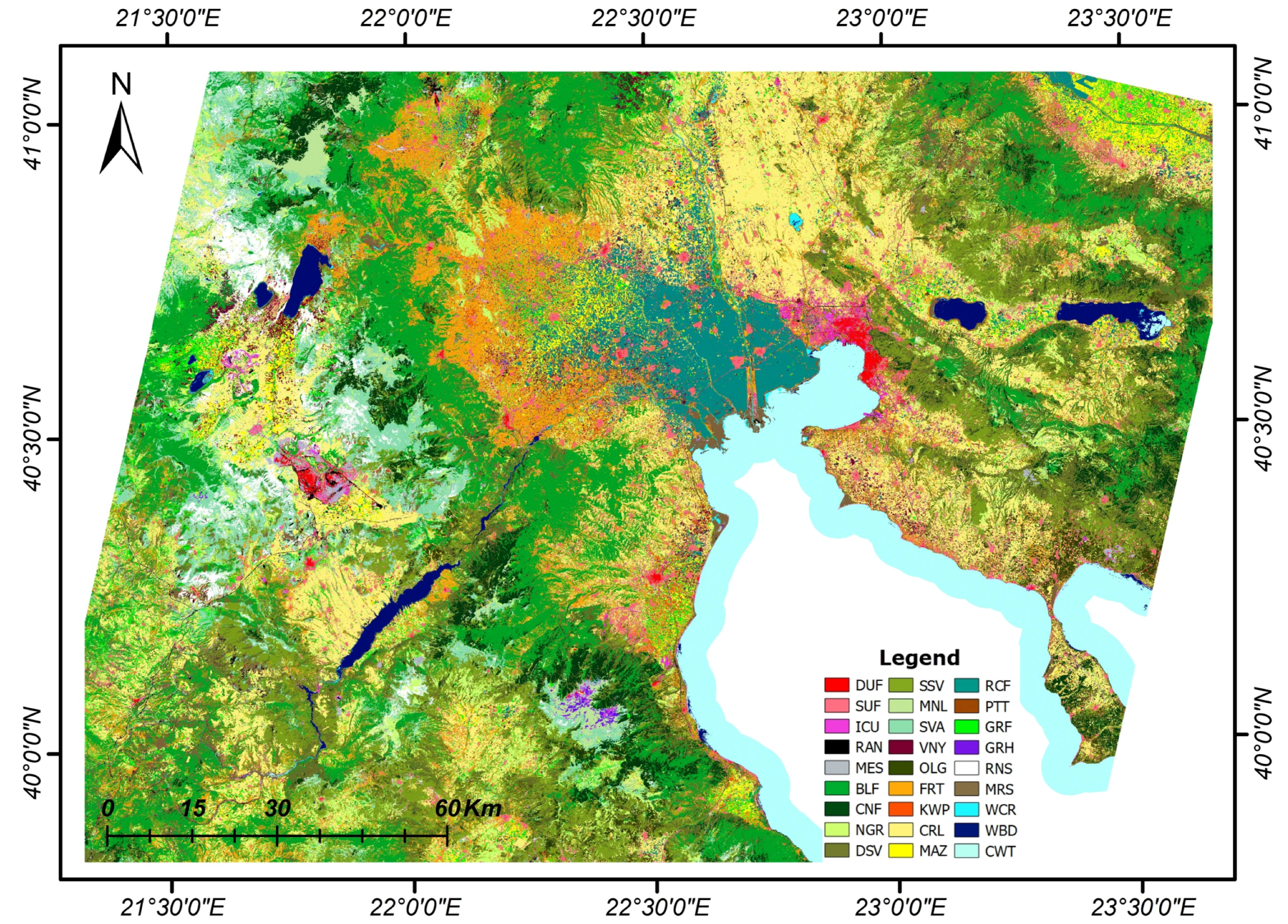
Following the comparative analysis between the different algorithms, datasets and features, in this section per-class performance and separability aspects are discussed based on the SVM experiment on the Dataset #2 with the top 70% of the employed features. This specific experiment presented the minimum number of classes with low PA, UA and F1 per-class scores (see Section 3.3 and Table 6). The resulting classification map is presented in Figure 8. Note that a water mask was computed based on the L8 QA band. It was then applied for marine waters with a buffer of 5 km in order to exclude the non-coastal marine waters from the prediction.

One can observe in Figure 8 that urban areas like the metropolitan area of Thessaloniki, as well as smaller towns like Katerini, Veria, Naoussa, Kozani and Ptolemaida have been accurately detected by the proposed classification framework (i.e., classes DUF, SUF and ICU) with a small extent of misclassification cases. Moreover, large inland water bodies such as Vegoritida, Polyfytos and Koroneia lakes have been successfully detected as well. In a few cases, certain pixels have been wrongly labelled as WCR (Pikrolimni Lake) or CWR (Volvi Lake). Regarding the performance over agricultural areas, in the northern region of Central Macedonia, which is characterized by vast cereal crop cultivation, the resulting detailed (in terms of number of classes) land cover map managed to correctly detected the CRL class as well as the extended rice cultivation regions (RCF class) around Axios and Aliakmonas River deltas.

In a similarly successful manner, the classification framework managed to detect and correctly label fruit tree cultivation areas (FRT class) around Naoussa, Veria and Edessa regions. Forest classes (BLF, CNF) were correctly reported on upland and mountainous areas, while Mediterranean-type evergreen sclerophyllous vegetation classes (DSV, SSV) were mapped on lowlands. Mountain massifs are also spotted with the presence of MNL, SVA and RNS classes. Certain classification errors are observed around Olympus Mountain where parts of bareland rocks usually covered by snow are classified as GRH. More detailed cases with classification errors are further discussed in Section 3.5.2.

3.5.1. Per-Class Quantitative Assessment

The aforementioned qualitative observations are in accordance with the reported quantitative results from the corresponding confusion matrix (

Table 7. The confusion matrix for the SVM classification framework (Dataset #2 on the top 70% of features). Columns represent classification labels and rows represent the testing data labels. Values are given in percentage (%) of testing pixels (normalised per row). Diagonal values express the PA for each class.

Confusion Matrix
	DUF	SUF	ICU	RAN	MES	BLF	CNF	NGR	DSV	SSV	MNL	SVA	VNY	OLG	FRT	KWP	CRL	MAZ	RCF	PTT	GRF	GRH	RNS	MRS	WCR	WBD	CWT
DUF	65.77	23.12	4.88	0.15	5.11	0.00	0.00	0.00	0.00	0.00	0.00	0.08	0.00	0.00	0.00	0.00	0.00	0.00	0.00	0.00	0.00	0.00	0.90	0.00	0.00	0.00	0.00
SUF	6.33	88.15	0.00	0.12	0.06	0.00	0.00	0.35	0.00	0.29	0.00	0.23	0.06	0.00	3.22	0.00	0.17	0.00	0.00	0.00	0.69	0.00	0.29	0.06	0.00	0.00	0.00
ICU	10.33	2.01	69.58	0.29	14.35	0.00	0.00	0.00	0.00	0.00	0.00	0.29	0.00	0.00	0.14	0.00	0.14	0.00	0.00	0.00	0.00	1.29	1.15	0.43	0.00	0.00	0.00
RAN	0.00	4.92	27.32	57.38	1.64	0.00	0.00	0.00	0.00	0.00	0.00	1.64	0.55	0.00	1.09	0.00	0.00	0.00	0.00	0.00	0.00	0.00	4.92	0.55	0.00	0.00	0.00
MES	1.34	5.45	22.77	0.63	49.17	0.00	0.00	0.00	0.00	0.00	0.00	0.00	0.00	0.00	0.00	0.00	0.00	0.00	0.00	0.00	0.00	0.00	20.63	0.00	0.00	0.00	0.00
BLF	0.00	0.00	0.00	0.00	0.00	86.24	9.40	0.61	1.15	1.47	0.12	0.11	0.00	0.05	0.00	0.05	0.00	0.00	0.00	0.00	0.78	0.00	0.00	0.02	0.00	0.00	0.00
CNF	0.00	0.00	0.00	0.00	0.08	4.29	88.03	0.00	6.48	0.24	0.03	0.03	0.00	0.63	0.00	0.00	0.00	0.00	0.00	0.00	0.00	0.00	0.00	0.21	0.00	0.00	0.00
NGR	0.00	0.00	0.00	0.00	0.00	0.00	0.00	75.08	0.34	3.03	0.00	0.00	0.00	1.01	1.35	0.00	0.00	0.00	0.00	0.00	2.02	0.00	17.17	0.00	0.00	0.00	0.00
DSV	0.00	0.00	0.00	0.00	0.00	33.54	40.87	0.00	24.63	0.24	0.00	0.00	0.00	0.72	0.00	0.00	0.00	0.00	0.00	0.00	0.00	0.00	0.00	0.00	0.00	0.00	0.00
SSV	0.00	0.16	0.00	0.00	0.00	2.27	0.00	6.97	16.55	55.47	0.00	10.95	0.00	4.22	0.24	0.00	0.00	0.00	0.00	0.00	0.57	0.00	0.00	2.60	0.00	0.00	0.00
MNL	0.00	0.00	0.00	0.00	7.80	0.00	0.00	5.42	0.00	0.00	63.05	12.54	0.00	0.00	0.00	0.00	2.71	0.00	0.00	0.00	7.46	1.02	0.00	0.00	0.00	0.00	0.00
SVA	0.00	0.00	0.00	0.00	1.57	0.00	0.00	0.00	0.00	16.44	4.70	68.30	0.00	0.00	0.39	0.00	0.00	0.00	0.00	0.00	1.37	0.00	7.05	0.20	0.00	0.00	0.00
VNY	0.00	26.21	0.00	0.00	0.00	0.00	0.00	0.00	0.00	0.18	0.00	0.00	57.63	0.18	10.23	0.00	0.36	0.54	4.13	0.00	0.54	0.00	0.00	0.00	0.00	0.00	0.00
OLG	0.00	4.96	0.00	0.00	0.00	1.53	0.00	2.29	2.67	15.65	0.00	0.00	0.38	56.11	15.27	0.00	0.00	0.00	0.00	0.00	1.15	0.00	0.00	0.00	0.00	0.00	0.00
FRT	0.00	3.24	0.00	0.00	0.00	2.00	0.00	0.92	0.00	2.47	0.00	0.00	3.39	3.39	64.10	8.78	2.31	0.31	0.77	0.00	8.17	0.00	0.00	0.15	0.00	0.00	0.00
KWP	0.00	0.00	0.00	0.00	0.00	0.00	0.00	0.00	0.00	0.00	0.00	0.00	0.00	0.00	0.33	99.67	0.00	0.00	0.00	0.00	0.00	0.00	0.00	0.00	0.00	0.00	0.00
CRL	0.00	0.24	0.00	0.00	0.00	0.00	0.00	3.06	0.00	1.18	0.00	0.00	0.12	0.00	1.18	0.00	92.95	0.00	0.00	0.00	0.94	0.00	0.00	0.35	0.00	0.00	0.00
MAZ	0.00	0.00	0.00	0.00	0.00	0.00	0.00	0.00	0.00	0.00	0.00	0.00	0.00	0.00	0.00	0.00	0.00	86.32	13.25	0.43	0.00	0.00	0.00	0.00	0.00	0.00	0.00
RCF	0.00	0.00	0.00	0.00	0.00	0.00	0.00	0.00	0.00	0.00	0.00	0.00	0.00	0.00	0.00	0.00	0.00	0.05	99.95	0.00	0.00	0.00	0.00	0.00	0.00	0.00	0.00
PTT	0.00	0.00	0.00	0.00	0.00	0.00	0.00	0.00	0.00	0.00	0.00	0.00	0.00	0.00	0.00	2.16	0.00	26.49	0.00	69.73	1.62	0.00	0.00	0.00	0.00	0.00	0.00
GRF	0.00	0.25	0.00	0.00	0.49	0.00	0.00	9.34	0.00	0.49	0.00	0.00	8.85	0.00	19.16	0.00	8.11	2.21	0.00	0.00	51.11	0.00	0.00	0.00	0.00	0.00	0.00
GRH	0.00	3.95	1.32	0.00	0.00	0.00	0.00	0.00	0.00	0.00	0.00	0.00	5.26	0.00	0.00	0.00	0.00	0.00	0.00	0.00	1.32	88.16	0.00	0.00	0.00	0.00	0.00
RNS	0.32	0.06	6.63	0.06	1.29	0.00	0.00	0.06	0.00	1.93	7.14	33.53	0.00	0.00	0.00	0.00	0.00	0.00	0.00	0.00	0.00	1.93	45.75	1.29	0.00	0.00	0.00
MRS	0.00	0.00	0.00	1.25	0.00	8.67	1.75	15.60	2.24	6.55	0.00	0.38	0.05	0.00	6.93	0.00	0.00	0.44	0.00	0.00	0.05	0.00	1.53	46.54	6.44	1.58	0.00
WCR	0.00	0.00	0.00	0.00	0.00	0.00	0.36	0.00	0.00	0.00	0.00	0.00	0.00	0.00	0.00	0.00	0.00	0.00	0.00	0.00	0.00	0.00	0.00	2.53	97.11	0.00	0.00
WBD	0.00	0.00	0.00	0.00	0.00	0.00	0.00	0.00	0.00	0.00	0.00	0.00	0.00	0.00	0.00	0.00	0.00	0.00	0.00	0.00	0.00	0.00	0.00	0.00	0.17	99.83	0.00
CWT	0.00	0.00	0.00	0.00	0.00	0.00	0.00	0.00	0.00	0.00	0.00	0.00	0.00	0.00	0.00	0.00	0.00	0.00	0.00	0.00	0.00	0.00	0.00	0.00	3.56	6.21	90.22
Number of testing pixels: 44,672
OA: 80.37%, Kappa: 77.93%

). Firstly, regarding the artificial terrain classes (i.e., DUF, SUF, ICU and RAN) that consist of sealed man-made surfaces, they overall achieved medium to high PA rates (57.38–88.15%) and in most cases they are confused between each other. The artificial terrain class MES resulted, also, into a number of classification errors mainly with ICU (23%) and RNS (21%). The spectral behaviour distinct characteristics among MES (open-pit extraction of minerals/ inert materials) and RNS (bare land areas, rock, cliffs and sand) were proven challenging to separate.

Concerning natural areas, BLF was detected with relatively high accuracy (PA: 86.24%) and was mainly confused with CNF, while the latter also achieved a high PA rate of approximately 88%, with a few cases of confusion with DSV and BLF. NGR areas were successfully detected with a PA rate of approximately 75%. The DSV class, corresponding to areas of dense bushy sclerophyllous vegetation, reported a lower PA rate. Approximately 34% and 41% of its testing pixels were classified as BLF and CNF, respectively. These classification errors involve three classes of dense woody vegetation that possess spectral similarities across the spectral–temporal datacube at a 30-m spatial scale. SSV achieved an average PA score (55.47%), presenting several mixing cases with DSV and SVA. High-altitude moor areas with moss and lichen, represented by class MNL, reported a PA rate of 63.05% and were mainly confused with areas of scattered vegetation (SVA). The latter hold a PA rate of 68.30% and in certain cases the testing samples (17%) were confused with SSV, a class also representing sparse vegetation.

The agricultural classes of KWP, CRL, MAZ, RCF, GRH were accurately classified at rates over 85%. VNY and OLG reported a medium PA rate of approximately 57%, since the first one presented mixings mainly with classes SUF and FRT and the second with SSV and FRT. Furthermore, FRT, which represents a heterogeneous land cover class including a variety of fruit trees and therefore patterns, texture, etc., was classified with a PA rate of 64.10%.

In particular, FRT presented confusions with a number of classes like KWP, VNY, OLG, GRF and SUF. The fact that permanent crop classes (i.e., VNY, OLG, FRT) presented misclassification error mixings not only with crop classes but also with SUF and SSV, can be attributed to similar spectral behaviour at this scale since those specific cultivation covers at a 30 m pixel include both vegetated (plants and trees) and non-vegetated (mainly soil) parts, similar to classes SUF and SSV. Another heterogeneous class, GRF, which includes grass fodder cultivations like clover and alfalfa, also presented some confusion (PA: approx. 51%) with FRT, VNY, CRL and NGR. On the other hand, PTT was detected with a relatively high PA rate (approx. 70%) and presented certain mixings with MAZ.

Bare land class RNS was evaluated with a lower PA of 45.75% as it presented mixings with many classes, especially with SVA and MNL, all mainly found in bare/semi-bare mountainous areas, but also to a smaller extent with high brightness man-made land covers like ICU and GRH. The MRS class, which includes low-lying land usually flooded by water and partially covered with herbaceous vegetation, presented a relatively low PA rate (46.5%). MRS was mainly confused with certain vegetation classes (e.g., NGR, BLF, SSV, FRT) but also with a few water classes, especially WCR. On the contrary, all water classes (i.e., WCR, WBD and CWT) were detected with high classification accuracy rates of over 90%.

3.5.2. Discussing Classification Errors in Challenging Cases

In this section, certain classification difficulties and misclassification cases are discussed in more detail. In particular, Figure 9a illustrates the challenges in separating MES areas that present high spatial, spectral and temporal heterogeneity and similar behaviour with a variety of terrain objects, materials and mixed covers. In this case (Figure 9a), one of the largest lignite reserves in Greece, the lignite mine of Ptolemais and the Ptolemais power plant area, are presented with a natural colour composite (RGB) from a L8 and Google Earth imagery. As can be observed in the resulting land cover map, apart from the MES class, the mining areas were also misclassified to other artificial terrain classes like DUF, SUF, ICU, RAN and also RNS due to similar spectral characteristics.

Another example with extended classification errors is presented in Figure 9b in the region of mountain Olympus. In particular, apart from MNL, SVA and RNS classes, all to be expected in high-altitude terrains, we also observe mapping of man-made classes MES, ICU and GRH. In particular, Mount Olympus, as the highest mountain of Greece and of our study area, presents snow and cloud coverage for a long period of the year, and therefore the higher intensity values across the spectrum for this area may have been confused with similar values of stable artificial surfaces classes. Moreover, this particular region was one of the areas participating in testing after the partition and thus no training data incorporating this seasonal information for alpine classes MNL, SVA and RNS were fed to the classifier. The latter emerges as a possible drawback of the strict approach of spatial partition of training and testing areas for the map production, especially for cases like this, i.e., semi-arid areas where the influence of lithological differences on the spectral response of a land cover class is not negligible. Nonetheless, partition was required for a direct quantitative comparison of the SVM with the CNN approach. In general, if we assessed solely the SVM framework validation, although a not-partitioned sampling procedure will not involve exactly the same samples in the learning and the testing process, it would undoubtedly include neighbours, probably leading to an overestimation of the calculated accuracy.

Another case of resulted classification errors is presented in Figure 9c. In particular, an agricultural area near Lake Vegora is presented where a variety of crop types are cultivated including vineyards, fruit trees, cereals, potatoes and maize. After a closer look, one can observe that several fruit parcels (FRT, marked with blue in the RGB images) have been wrongly classified as VNY. At this particular spatial scale (30 m), where linear against dot pattern characteristics cannot be effectively recorded, the crop types of similar spectral and temporal (phenological) behaviour were not distinguished successfully by the classifier in many cases and thus presented mixings between them.

4. Conclusions

In this paper, we introduced a framework for the systematic, detailed land cover mapping from annual high-resolution satellite data. The main contribution of our approach lies in the assessment of the influence of cloud cover on the classification of multitemporal datasets, composed of images with different cloud cover levels. Moreover, we performed detailed mapping in terms of targeting to discriminate between more than 25 land cover classes. The developed nomenclature contained 27 classes, based mainly on CLC Level-3 classes and several additional crop types. The annual satellite L8 data were formed into different spatio–spectro–temporal datacubes and a machine learning classifier with either a shallow (SVM) or a deeper architecture (CNN) was applied for the classification procedure. Quantitatively, the resulting overall accuracy rates differed by less than 3%. However, the SVM classification framework was less computationally demanding and produced more accurate results across class boundaries. The highest overall accuracy rates (above 80%) were derived for multitemporal datasets with up to 20–30% cloud cover. The feature selection procedure was proven beneficial for most cases. Regarding the influence of cloud presence on the training and testing data, our experiments indicated that a cloud cover of over 25% per class resulted in lower F1 rates. However, a direct correlation between cloud presence (in the reference data) and the resulting per-class accuracy was not observed. This fact highlights that the combination of the employed features along with the distinct spectral and/or phenological characteristics of each class determine how successful the classification would be. These promising results indicate that operational classification frameworks can be developed for detailed land cover mapping on an annual basis. Towards the latter, the optimal integration of topographic, climate and microclimate information in the framework is an open matter and can address the different phenological patterns of vegetation, which currently are modelled during the training procedure as a variation among labelled features. The contribution of additional temporal features (e.g., day of year with the max value of a vegetation index) that are not correlated with clouds will be also assessed.

References

- Bojinski, S.; Verstraete, M.; Peterson, T.C.; Richter, C.; Simmons, A.; Zemp, M. The Concept of Essential Climate Variables in Support of Climate Research, Applications, and Policy. Bull. Am. Meteorol. Soc. 2014, 95, 1431–1443. [Google Scholar] [CrossRef] [Green Version]
- Gong, P.; Wang, J.; Yu, L.; Zhao, Y.; Zhao, Y.; Liang, L.; Niu, Z.; Huang, X.; Fu, H.; Liu, S.; et al. Finer resolution observation and monitoring of global land cover: First mapping results with Landsat TM and ETM+ data. Int. J. Remote Sens. 2013, 34, 2607–2654. [Google Scholar] [CrossRef]
- Yu, L.; Wang, J.; Li, X.; Li, C.; Zhao, Y.; Gong, P. A multi-resolution global land cover dataset through multisource data aggregation. Sci. China Earth Sci. 2014, 57, 2317–2329. [Google Scholar] [CrossRef]
- Chen, J.; Chen, J.; Liao, A.; Cao, X.; Chen, L.; Chen, X.; He, C.; Han, G.; Peng, S.; Lu, M.; et al. Global land cover mapping at 30 m resolution: A POK-based operational approach. ISPRS J. Photogramm. Remote Sens. 2015, 103, 7–27. [Google Scholar] [CrossRef]
- Homer, C. Completion of the 2001 National Land Cover Database for the Conterminous United States. Photogramm. Eng. Remote Sens. 2007, 73, 337–341. [Google Scholar]
- Inglada, J.; Vincent, A.; Arias, M.; Tardy, B.; Morin, D.; Rodes, I. Operational high resolution land cover map production at the country scale using satellite image time series. Remote Sens. 2017, 9, 95. [Google Scholar] [CrossRef]
- Xiong, J.; Thenkabail, P.S.; Tilton, J.C.; Gumma, M.K.; Teluguntla, P.; Oliphant, A.; Congalton, R.G.; Yadav, K.; Gorelick, N. Nominal 30-m Cropland Extent Map of Continental Africa by Integrating Pixel-Based and Object-Based Algorithms Using Sentinel-2 and Landsat-8 Data on Google Earth Engine. Remote Sens. 2017, 9, 1065. [Google Scholar] [CrossRef]
- Pelletier, C.; Valero, S.; Inglada, J.; Champion, N.; Dedieu, G. Assessing the robustness of Random Forests to map land cover with high resolution satellite image time series over large areas. Remote Sens. Environ. 2016, 187, 156–168. [Google Scholar] [CrossRef]
- Inglada, J.; Arias, M.; Tardy, B.; Hagolle, O.; Valero, S.; Morin, D.; Dedieu, G.; Sepulcre, G.; Bontemps, S.; Defourny, P.; et al. Assessment of an operational system for crop type map production using high temporal and spatial resolution satellite optical imagery. Remote Sens. 2015, 7, 12356–12379. [Google Scholar] [CrossRef]
- Marais Sicre, C.; Inglada, J.; Fieuzal, R.; Baup, F.; Valero, S.; Cros, J.; Huc, M.; Demarez, V. Early Detection of Summer Crops Using High Spatial Resolution Optical Image Time Series. Remote Sens. 2016, 8, 591. [Google Scholar] [CrossRef]
- Belgiu, M.; Csillik, O. Sentinel-2 cropland mapping using pixel-based and object-based time-weighted dynamic time warping analysis. Remote Sens. Environ. 2018, 204, 509–523. [Google Scholar] [CrossRef]
- Rogan, J.; Franklin, J.; Roberts, D.A. A comparison of methods for monitoring multitemporal vegetation change using Thematic Mapper imagery. Remote Sens. Environ. 2002, 80, 143–156. [Google Scholar] [CrossRef] [Green Version]
- Rodriguez-Galiano, V.F.; Ghimire, B.; Rogan, J.; Chica-Olmo, M.; Rigol-Sanchez, J.P. An assessment of the effectiveness of a random forest classifier for land-cover classification. ISPRS J. Photogramm. Remote Sens. 2012, 67, 93–104. [Google Scholar] [CrossRef]
- Whitcraft, A.K.; Vermote, E.F.; Becker-Reshef, I.; Justice, C.O. Cloud cover throughout the agricultural growing season: Impacts on passive optical earth observations. Remote Sens. Environ. 2015, 156, 438–447. [Google Scholar] [CrossRef]
- Banskota, A.; Kayastha, N.; Falkowski, M.J.; Wulder, M.A.; Froese, R.E.; White, J.C. Forest Monitoring Using Landsat Time Series Data: A Review. Can. J. Remote Sens. 2014, 40, 362–384. [Google Scholar] [CrossRef]
- Valero, S.; Morin, D.; Inglada, J.; Sepulcre, G.; Arias, M.; Hagolle, O.; Dedieu, G.; Bontemps, S.; Defourny, P.; Koetz, B. Production of a Dynamic Cropland Mask by Processing Remote Sens. Image Series at High Temporal and Spatial Resolutions. Remote Sens. 2016, 8, 55. [Google Scholar] [CrossRef]
- Hansen, M.C.; Loveland, T.R. A review of large area monitoring of land cover change using Landsat data. Remote Sens. Environ. 2012, 122, 66–74. [Google Scholar] [CrossRef]
- Khatami, R.; Mountrakis, G.; Stehman, S.V. A meta-analysis of remote sensing research on supervised pixel-based land-cover image classification processes: General guidelines for practitioners and future research. Remote Sens. Environ. 2016, 177, 89–100. [Google Scholar] [CrossRef] [Green Version]
- Vapnik, V.N. The Nature of Statistical Learning Theory; Springer: New York, NY, USA, 1995; ISBN 978-1-4757-2440-0. [Google Scholar]
- Vapnik, V. Statistical Learning Theory; Wiley: New York, NY, USA, 1998. [Google Scholar]
- Breiman, L. Random forests. Mach. Learn. 2001, 45, 5–32. [Google Scholar] [CrossRef]
- Pelletier, C.; Valero, S.; Inglada, J.; Champion, N.; Marais Sicre, C.; Dedieu, G. Effect of Training Class Label Noise on Classification Performances for Land Cover Mapping with Satellite Image Time Series. Remote Sens. 2017, 9, 173. [Google Scholar] [CrossRef]
- Zheng, B.; Myint, S.W.; Thenkabail, P.S.; Aggarwal, R.M. A support vector machine to identify irrigated crop types using time-series Landsat NDVI data. Int. J. Appl. Earth Obs. Geoinf. 2015, 34, 103–112. [Google Scholar] [CrossRef]
- Peña, M.A.; Brenning, A. Assessing fruit-tree crop classification from Landsat-8 time series for the Maipo Valley, Chile. Remote Sens. Environ. 2015, 171, 234–244. [Google Scholar] [CrossRef]
- Paneque-Gálvez, J.; Mas, J.-F.; Moré, G.; Cristóbal, J.; Orta-Martínez, M.; Luz, A.C.; Guèze, M.; Macía, M.J.; Reyes-García, V. Enhanced land use/cover classification of heterogeneous tropical landscapes using support vector machines and textural homogeneity. Int. J. Appl. Earth Obs. Geoinf. 2013, 23, 372–383. [Google Scholar] [CrossRef]
- Karantzalos, K.; Bliziotis, D.; Karmas, A. A scalable geospatial web service for near real-time, high-resolution land cover mapping. IEEE J. Sel. Top. Appl. Earth Obs. Remote Sens. 2015, 8, 4665–4674. [Google Scholar] [CrossRef]
- Mountrakis, G.; Im, J.; Ogole, C. Support vector machines in remote sensing: A review. ISPRS J. Photogramm. Remote Sens. 2011, 66, 247–259. [Google Scholar] [CrossRef]
- Shao, Y.; Lunetta, R.S. Comparison of support vector machine, neural network, and CART algorithms for the land-cover classification using limited training data points. ISPRS J. Photogramm. Remote Sens. 2012, 70, 78–87. [Google Scholar] [CrossRef]
- Foody, G.M.; Mathur, A. Toward intelligent training of supervised image classifications: Directing training data acquisition for SVM classification. Remote Sens. Environ. 2004, 93, 107–117. [Google Scholar] [CrossRef]
- Foody, G.M.; Mathur, A. The use of small training sets containing mixed pixels for accurate hard image classification: Training on mixed spectral responses for classification by a SVM. Remote Sens. Environ. 2006, 103, 179–189. [Google Scholar] [CrossRef]
- Gómez, C.; White, J.C.; Wulder, M.A. Optical remotely sensed time series data for land cover classification: A review. ISPRS J. Photogramm. Remote Sens. 2016, 116, 55–72. [Google Scholar] [CrossRef]
- Belgiu, M.; Drăguţ, L. Random forest in remote sensing: A review of applications and future directions. ISPRS J. Photogramm. Remote Sens. 2016, 114, 24–31. [Google Scholar] [CrossRef]
- Sharma, A.; Liu, X.; Yang, X.; Shi, D. A patch-based convolutional neural network for remote sensing image classification. Neural Netw. 2017, 95, 19–28. [Google Scholar] [CrossRef] [PubMed]
- Papadomanolaki, M.; Vakalopoulou, M.; Zagoruyko, S.; Karantzalos, K. Benchmarking deep learning frameworks for the classification of very high resolution satellite multispectral data. ISPRS Ann. Photogramm. Remote Sens. Spat. Inf. Sci. 2016, 7, 83–88. [Google Scholar] [CrossRef]
- Volpi, M.; Tuia, D. Dense semantic labeling of subdecimeter resolution images with convolutional neural networks. IEEE Trans. Geosci. Remote Sens. 2017, 55, 881–893. [Google Scholar] [CrossRef]
- Kussul, N.; Lavreniuk, M.; Skakun, S.; Shelestov, A. Deep learning classification of land cover and crop types using remote sensing data. IEEE Trans. Geosci. Remote Sens. Lett. 2017, 14, 778–782. [Google Scholar] [CrossRef]
- Maggiori, E.; Tarabalka, Y.; Charpiat, G.; Alliez, P. High-Resolution Aerial Image Labeling With Convolutional Neural Networks. IEEE Trans. Geosci. Remote Sens. 2017, 55, 7092–7103. [Google Scholar] [CrossRef] [Green Version]
- Papadomanolaki, M.; Vakalopoulou, M.; Karantzalos, K. Patch-based deep learning architectures for sparse annotated very high resolution datasets. In Proceedings of the Urban Remote Sensing Event (JURSE), 2017 Joint, Dubai, UAE, 6–8 March 2017; IEEE: Piscataway, NJ, USA, 2017; pp. 1–4. [Google Scholar]
- Rußwurm, M.; Körner, M. Multi-Temporal Land Cover Classification with Long Short-Term Memory Neural Networks. Int. Arch. Photogramm. Remote Sens. Spat. Inf. Sci. 2017, 42, 551. [Google Scholar] [CrossRef]
- Dixon, B.; Candade, N. Multispectral landuse classification using neural networks and support vector machines: One or the other, or both? Int. J. Remote Sens. 2008, 29, 1185–1206. [Google Scholar] [CrossRef]
- Peel, M.C.; Finlayson, B.L.; McMahon, T.A. Updated world map of the Köppen-Geiger climate classification. Hydrol. Earth Syst. Sci. Discuss. 2007, 4, 439–473. [Google Scholar] [CrossRef]
- Köppen, W.; Volken, E.; Brönnimann, S. Die Wärmezonen der Erde, nach der Dauer der heissen, gemässigten und kalten Zeit und nach der Wirkung der Wärme auf die organische Welt betrachtet, Meteorol. Z. 1884, 1, 215–226; reprinted in The thermal zones of the earth according to the duration of hot, moderate and cold periods and to the impact of heat on the organic world. Meteorol. Z. 2011, 20, 351–360. [Google Scholar]
- Karakizi, C.; Vakalopoulou, M.; Karantzalos, K. Annual Crop-type Classification from Multitemporal Landsat-8 and Sentinel-2 Data based on Deep-learning. In Proceedings of the 37th International Symposium on Remote Sensing of Environment (ISRSE-37), Tshwane, South Africa, 8–12 May 2017. [Google Scholar]
- Karakizi, C.; Karantzalos, K. Comparing Land Cover Maps derived from all Annual Landsat-8 and Sentinel-2 Data at Different Spatial Scales. In Proceedings of the ESA WorldCover Conference, Frascati, Rome, Italy, 14–16 March 2017. [Google Scholar]
- Zhu, Z.; Wang, S.; Woodcock, C.E. Improvement and expansion of the Fmask algorithm: Cloud, cloud shadow, and snow detection for Landsats 4–7, 8, and Sentinel 2 images. Remote Sens. Environ. 2015, 159, 269–277. [Google Scholar] [CrossRef]
- European Environment Agency (EEA) under the Framework of the Copernicus Programme CORINE Land Cover Nomenclature. Available online: https://land.copernicus.eu/user-corner/technical-library/corine-land-cover-nomenclature-guidelines/docs/pdf/CLC2018_Nomenclature_illustrated_guide_20170930.pdf (accessed on 30 July 2018).
- Shih, H.; Stow, D.A.; Weeks, J.R.; Coulter, L.L. Determining the Type and Starting Time of Land Cover and Land Use Change in Southern Ghana Based on Discrete Analysis of Dense Landsat Image Time Series. IEEE J. Sel. Top. Appl. Earth Obs. Remote Sens. 2016, 9, 2064–2073. [Google Scholar] [CrossRef]
- Müller, H.; Rufin, P.; Griffiths, P.; Siqueira, A.J.B.; Hostert, P. Mining dense Landsat time series for separating cropland and pasture in a heterogeneous Brazilian savanna landscape. Remote Sens. Environ. 2015, 156, 490–499. [Google Scholar] [CrossRef] [Green Version]
- Yeom, J.; Han, Y.; Kim, Y. Separability analysis and classification of rice fields using KOMPSAT-2 High Resolution Satellite Imagery. Res. J. Chem. Environ. 2013, 17, 136–144. [Google Scholar]
- Rouse, J., Jr.; Haas, R.H.; Schell, J.A.; Deering, D.W. Monitoring Vegetation Systems in the Great Plains with ERTS; Goddard Space Flight Center: Greenbelt, MD, USA, 1974. [Google Scholar]
- Qi, J.; Chehbouni, A.; Huete, A.R.; Kerr, Y.H.; Sorooshian, S. A modified soil adjusted vegetation index. Remote Sens. Environ. 1994, 48, 119–126. [Google Scholar] [CrossRef]
- Gao, B.-C. NDWI—A normalized difference water index for remote sensing of vegetation liquid water from space. Remote Sens. Environ. 1996, 58, 257–266. [Google Scholar] [CrossRef]
- Zha, Y.; Gao, J.; Ni, S. Use of normalized difference built-up index in automatically mapping urban areas from TM imagery. Int. J. Remote Sens. 2003, 24, 583–594. [Google Scholar] [CrossRef]
- Congalton, R.G.; Green, K. Assessing the Accuracy of Remotely Sensed Data: Principles and Practices; CRC Press: Boca Raton, FL, USA, 2008. [Google Scholar]
- Kinkeldey, C. A concept for uncertainty-aware analysis of land cover change using geovisual analytics. ISPRS Int. J. Geo-Inf. 2014, 3, 1122–1138. [Google Scholar] [CrossRef]
- Chang, C.-C.; Lin, C.-J. LIBSVM: A Library for Support Vector Machines. ACM Trans. Intell. Syst. Technol. 2011, 2, 27. [Google Scholar] [CrossRef]
- Schölkopf, B.; Smola, A.J. Learning with Kernels: Support Vector Machines, Regularization, Optimization, and Beyond; MIT Press: Cambridge, MA, USA, 2002. [Google Scholar]
- Hsu, C.-W.; Chang, C.-C.; Lin, C.-J. A Practical Guide to Support Vector Classification; Department of Computer Science, National Taiwan University: Taipei, Taiwan, 2003. [Google Scholar]
- Marcos, D.; Volpi, M.; Kellenberger, B.; Tuia, D. Land cover mapping at very high resolution with rotation equivariant CNNs: Towards small yet accurate models. ISPRS J. Photogramm. Remote Sens. 2018. [Google Scholar] [CrossRef]
- Guyon, I.; Elisseeff, A. An introduction to variable and feature selection. J. Mach. Learn. Res. 2003, 3, 1157–1182. [Google Scholar]
- Yao, C.; Liu, Y.-F.; Jiang, B.; Han, J.; Han, J. LLE score: A new filter-based unsupervised feature selection method based on nonlinear manifold embedding and its application to image recognition. IEEE Trans. Image Process. 2017, 26, 5257–5269. [Google Scholar] [CrossRef] [PubMed]
- Wu, B.; Zhang, L.; Zhao, Y. Feature selection via Cramer’s V-test discretization for remote-sensing image classification. IEEE Trans. Geosci. Remote Sens. 2014, 52, 2593–2606. [Google Scholar] [CrossRef]
- Gnana, D.A.A.; Balamurugan, S.A.A.; Leavline, E.J. Literature review on feature selection methods for high-dimensional data. Int. J. Comput. Appl. 2016, 136. [Google Scholar] [CrossRef]
- Gu, Q.; Li, Z.; Han, J. Generalized fisher score for feature selection. arXiv, 2012; arXiv:1202.3725. Available online: https://arxiv.org/abs/1202.3725(accessed on 30 July 2018).
- Wang, D.; Hollaus, M.; Pfeifer, N. Feasibility of machine learning methods for separating wood and leaf points from terrestrial laser scanning data. ISPRS Ann. Photogramm. Remote Sens. Spat. Inf. Sci. 2017, 4, 157–164. [Google Scholar] [CrossRef]
- Jaganathan, P.; Rajkumar, N.; Kuppuchamy, R. A comparative study of improved F-score with support vector machine and RBF network for breast cancer classification. Int. J. Mach. Learn. Comput. 2012, 2, 741. [Google Scholar] [CrossRef]
- Chang, Y.-W.; Lin, C.-J. Feature Ranking Using Linear SVM. Proc. Mach. Learn. Res. 2008, 3, 53–64. Available online: http://proceedings.mlr.press/v3/chang08a/chang08a.pdf (accessed on 30 July 2018).
- Chen, Y.-W.; Lin, C.-J. Combining SVMs with various feature selection strategies. In Feature Extraction; Springer: New York, NY, USA, 2006; pp. 315–324. [Google Scholar]
- Congalton, R.G. A review of assessing the accuracy of classifications of remotely sensed data. Remote Sens. Environ. 1991, 37, 35–46. [Google Scholar] [CrossRef]
- Foody, G.M. Thematic Map Comparison: Evaluating the Statistical Significance of Differences in Classification Accuracy. Photogramm. Eng. Remote Sens. 2004, 70, 627–633. [Google Scholar] [CrossRef]
- Dash, J.; Mathur, A.; Foody, G.M.; Curran, P.J.; Chipman, J.W.; Lillesand, T.M. Land cover classification using multi-temporal MERIS vegetation indices. Int. J. Remote Sens. 2007, 28, 1137–1159. [Google Scholar] [CrossRef]
- Yan, L.; Roy, D.P. Conterminous United States crop field size quantification from multi-temporal Landsat data. Remote Sens. Environ. 2016, 172, 67–86. [Google Scholar] [CrossRef]
- Barsi, J.A.; Lee, K.; Kvaran, G.; Markham, B.L.; Pedelty, J.A. The spectral response of the Landsat-8 operational land imager. Remote Sens. 2014, 6, 10232–10251. [Google Scholar] [CrossRef]
Figure 1.
The study area is located in northern Greece, as can be seen in a natural color Landsat-8 (L8) composite from year 2016 (left) and covers an area of about 26,000 km2. The study area was partitioned in order to form independent training and testing datasets: training blocks are pictured in yellow, while testing ones with a cyan (right).
Figure 2.
The cloud frequency per pixel i.e., the number of cloudy dates for datasets: (a) #1 of total 11 dates, (b) #2 of total 14 dates, (c) #3 of total 16 dates and (d) #4 of total 18 dates. Regions in white represent clear pixels for all dates.
Figure 3.
A flowchart of the proposed classification framework and performed SVM experiments with Landsat-8 (L8) datasets of different cloud cover (CC) and additional feature selection (Feat. Sel.).
Figure 4.
The architecture of the CNN model for the classification of Dataset #1.
Figure 5.
Part of the resulting linear SVM (top left) and CNN (top right) land cover maps for Dataset #1. Bottom: their difference (black) and the reference data for this particular region (approx. 2,000 km2) are presented.
Figure 6.
Accuracy metrics for the SVM experiments on the four different cloud cover datasets.
Figure 7.
The per-class F1 scores (%) are illustrated in the bar chart for every dataset. The average per-class cloud cover (%) of the reference data are illustrated with dotted lines for every dataset.
Figure 8.
The classified map of the study area using 14 images/dates of cloud cover up to 30% after feature selection on 70% of top-ranked features for the 27 land cover classes with an OA of 80.4%.
Figure 9.
Indicative cases with classification errors regarding: (a) the MES land cover class, (b) the MNL, SVA and RNS classes and (c) parcels of the FRT class (outlined with blue).