Quality Improvement of Satellite Soil Moisture Products by Fusing with In-Situ Measurements and GNSS-R Estimates in the Western Continental U.S.

Abstract

Soil moisture is a key component of the water cycle budget. Sensing soil moisture using microwave sensors onboard satellites is an effective way to retrieve surface soil moisture (SSM) at a global scale, but the retrieval accuracy in some regions is inadequate due to the complicated factors influencing the general retrieval process. On the other hand, monitoring soil moisture directly through in-situ devices is capable of providing high-accuracy SSM measurements, but the distribution of such stations is sparse. Recently, the Global Navigation Satellite System interferometric Reflectometry (GNSS-R) method was used to derive field-scale SSM, which can serve as a supplement to contemporary sparse in-situ soil moisture networks. On this basis, it is of great research significance to explore the fusion of these different kinds of SSM data, so as to improve the present satellite SSM products with regard to their data accuracy. In this paper, a multi-source point-surface fusion method based on the generalized regression neural network (GRNN) model is applied to fuse the Soil Moisture Active Passive (SMAP) Level 3 radiometer SSM daily product with in-situ measured and GNSS-R estimated SSM data from five soil moisture networks in the western continental U.S. The results show that the GRNN model obtains a fairly good performance, with a cross-validation R value of approximately 0.9 and a ubRMSE of 0.044 cm³ cm⁻³. Furthermore, the fused SSM product agrees well with the site-specific SSM data in terms of time and space, which demonstrates that the proposed GRNN model is able to construct the non-linear relationship between the point- and surface-scale SSM.

1. Introduction

Soil moisture is one of the key variables in the global water budget and water cycle. In particular, quantifying the magnitude and dynamics of surface soil moisture (SSM, defined as the moisture content of the top ~5 cm depth of soil) storage is essential for many practical reasons [1]. SSM can affect weather patterns [2], drought, and flooding [3,4], and plays an important role in climate change [2,5,6], plant growth [7,8], crop yield [9], etc. As a consequence, monitoring the long-term changes in SSM at large scales is crucial for hydrology, climatology, and agriculture.

Remote sensing using sensors onboard satellites is one of the most effective ways to derive a regional and/or global SSM map. In particular, microwave remote sensing is the most commonly used method for long-term and large-scale soil moisture monitoring due to its all-weather and all-time sensing ability. It was not until the 1970s that Ref. [10] qualitatively demonstrated the sensitivity of microwave brightness temperature to soil moisture variations. Since then, microwave remote sensing approaches using radiometers and/or scatterometers for soil moisture monitoring have been widely investigated, and a series of satellite-based microwave sensors operating at sub-optimal frequencies for SSM sensing have been applied to generate global SSM products spanning the last few decades, including both passive (e.g., SMMR, SSM/I, TRMM TMI, AMSR-E, WindSat, and AMSR2) and active (e.g., ERS-SCAT and MetOp ASCAT) microwave sensors. In 2009, the European Space Agency (ESA) launched the first dedicated soil moisture mission, the Soil Moisture and Ocean Salinity (SMOS) Earth Explorer, following which the National Aeronautics and Space Administration (NASA) launched the Soil Moisture Active Passive (SMAP) mission in 2015. These two dedicated soil moisture missions both carry instruments of the optimal L-band for sensing SSM, to produce long-term and large-scale SSM products with the accuracy requirement of 0.04 cm³ cm⁻³ volumetric soil moisture unbiased root-mean-square error (ubRMSE) [11,12].

Microwave remote sensing soil moisture products have been shown to be generally useful and accurate by extensive validation studies [13,14,15,16,17], either through direct comparison against in-situ measurements, or inter-comparison among different remotely sensed products. In addition, the applications of these products have also been widely explored in many fields like agriculture, hydrology, and climate sciences [18,19,20,21]. However, the general soil moisture retrieval process is significantly subject to uncertainties. First, because the emissive and scattering characteristics of the soil surface not only depend on the soil moisture content, but also other attributes such as land surface temperature, roughness, and vegetation characteristics, soil moisture retrievals from microwave satellite remote sensing are vulnerable to errors arising from these ancillary (i.e., “non-soil-moisture”) effects [22] and are also affected by other error sources including antenna noise and radio frequency interference (RFI). Therefore, the nominal retrievals derived from microwave satellite remote sensing have to be interpreted with caution as they contain pixels with surface/instrument conditions (e.g., mountainous terrain, dense vegetation, RFI, and frozen ground) that can lead to inaccurate soil moisture retrievals [23]. Secondly, current retrieval algorithms often rely on the empirical models originating from a few validation sites at a local scale, due to a lack of ancillary and heterogeneity information. For example, several retrieval algorithms usually use vegetation models formulated and calibrated from limited validation sites [24,25]. Therefore, they may have regional dependence and experience significant uncertainties outside these regions. For this reason, it is important to improve the quality of the satellite-derived SSM products to minimize the uncertainties.

On the other hand, monitoring soil moisture directly through in-situ devices is able to provide high-accuracy ground-level soil moisture measurements at various depths, and numerous small-scale (<100² km²) and large-scale (>100² km²) soil moisture networks [26,27] have been established at state and national levels over the past few decades. Nevertheless, these networks primarily serve as the calibration and validation of microwave remote sensing data, as the station distributions of these networks are too sparse to produce soil moisture maps at regional to global scales. Recently, a new kind of environmental sensing technique [28] in long-term soil moisture monitoring has emerged, which makes use of the interference of the direct and reflected Global Navigation Satellite System (GNSS) signals received by GNSS receivers mounted fairly close to the land surface. As such, the method is often referred to as GNSS interferometric reflectometry (GNSS-R). Essentially, GNSS-R is also within the category of microwave remote sensing as it detects the physical characteristics of an area by measuring its reflected radiation in the microwave wavelength region (L-band). The GNSS-R technique is able to retrieve SSM at a field scale (~1000 m²), and the validation of GNSS-R soil moisture retrievals (e.g., [29,30]) has demonstrated that the RMSE between GNSS-R-derived SSM and in-situ measurements could be less than 0.04 cm³ cm⁻³ in both bare and vegetated soil when vegetation effects were removed for vegetated soil. Because the GNSS-R technique is able to provide field-scale SSM estimates instead of typical point-scale measurements, and the fact that GNSS signals belong to the L-band, which is consistent with L-band microwave satellites, GNSS-R-based in-situ sites are being employed as excellent support for satellite soil moisture validation (e.g., a SMAP calibration/validation plan [31]). Therefore, the GNSS-R technique can serve as a supplement to contemporary sparse in-situ soil moisture networks. As a matter of fact, the GNSS-R-based soil moisture network named PBO H2O [32] was incorporated into the International Soil Moisture Network (ISMN) [33,34] in 2014.

Since these different soil moisture monitoring methods possess complementary advantages, recent studies have started to explore multi-source SSM data fusion between optical remote sensing soil moisture and ground-based observations. For instance, Ref. [35] successfully reconstructed optical satellite GF-1 soil moisture observations under full cloud contamination, based on satellite and in-situ sensor collaboration, demonstrated that in-situ sensors can be regarded as an important data source in effective environmental monitoring. On this basis, a subsequent study took an artificial neural network (ANN) as a reconstruction model instead of the conventional model to reconstruct GF-1 soil moisture observations under full cloud contamination [36]. The results indicated that the complex and highly variable relationships between the in-situ observations and optical remote sensing soil moisture were better projected using the ANN. However, to date, few works have looked into the study of multi-source data fusion in terms of microwave satellite remote sensing SSM. To our knowledge, Ref. [37] preliminarily proposed an algorithm using in-situ measurements from two sparse networks for training a neural network to retrieve SSM from SMOS brightness temperature observations, which did not give consideration to the GNSS-R-based soil moisture network. Therefore, it is of great research significance to explore the fusion of the aforementioned different kinds of SSM datasets (i.e., microwave satellite, in-situ, and GNSS-R), so as to improve the present satellite SSM products with regard to their data accuracy.

In this paper, a multi-source point-surface fusion method based on the generalized regression neural network (GRNN) model is applied to fuse microwave satellite SSM products with in-situ SSM measurements, as well as GNSS-R SSM estimates. The core idea of this study is to use the GRNN model to establish the non-linear relationship between the satellite-derived SSM and the “site-specific” (both in-situ and GNSS-R) SSM data, taking the site-specific SSM data as the training target. Then, after comprehensive evaluation of the fusion model performance, the trained GRNN model is applied to correct the original satellite SSM product, to generate quality-improved SSM maps.

The rest of this paper is organized as follows. Section 2 introduces the study area in detail. The SSM and other auxiliary data used for the fusion scheme and data pre-processing procedure are also described. Section 3 expounds the GRNN model structure, the two phases of the GRNN fusion approach, and the cross-validation technique. Section 4 comprehensively examines the GRNN model performance and presents the quality-improved SSM maps. The merit of incorporating the GNSS-R network in the fusion process is also discussed. Section 5 delivers the conclusion of the paper and provides an outlook for future research.

2. Study Area and Data

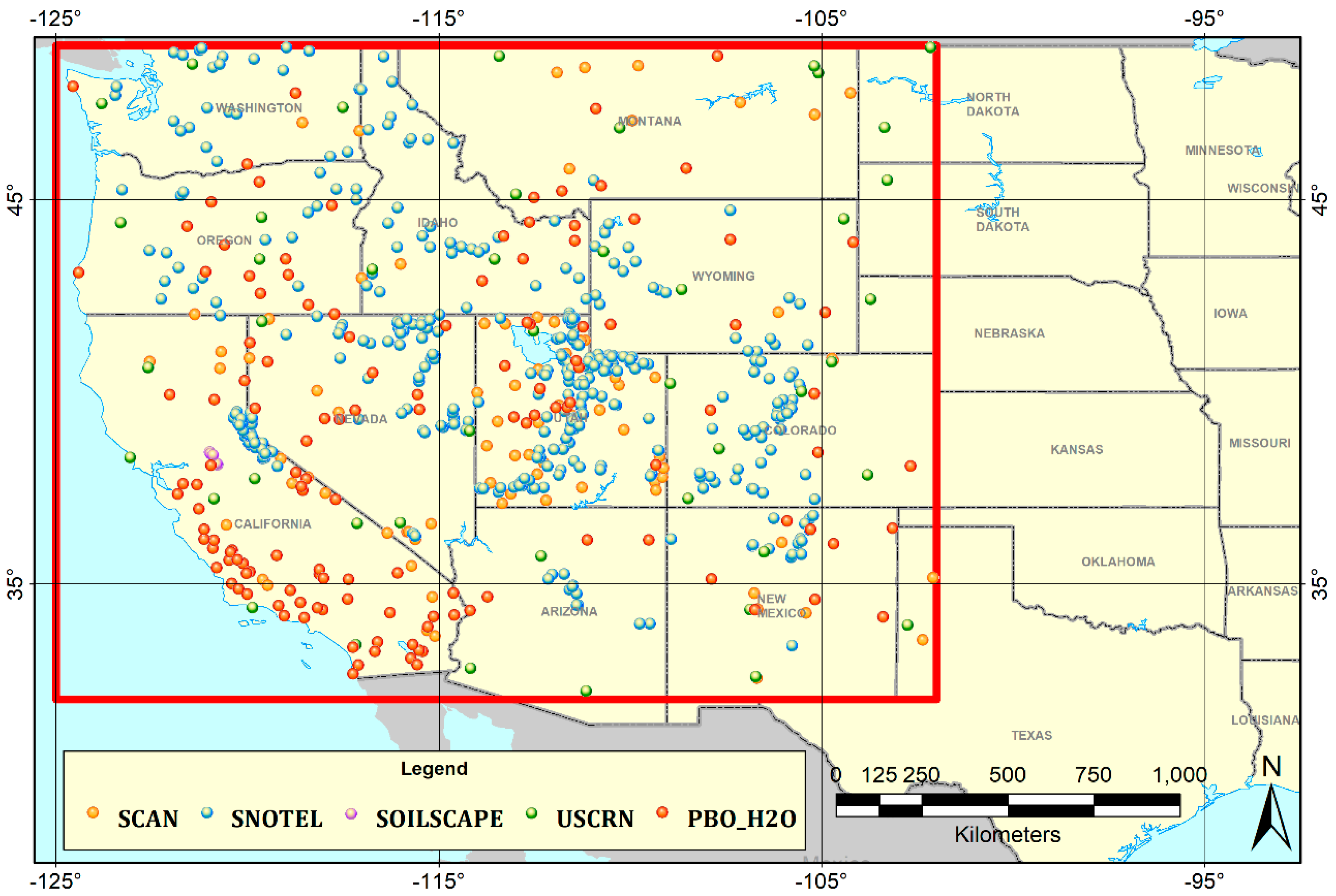
2.1. Study Area

The study area of our research was the western part of the Continental U.S. (CONUS). Specifically, we constrained the range of the latitude and longitude to 32°N–49°N and 125°W–102°W, as shown in the red rectangle in Figure 1.

There are several reasons why we restricted the study area to such a rigid range. First and most importantly, while in-situ networks are spread across the whole of the CONUS, nearly all of the GNSS sites used for soil moisture monitoring only belong to this region (Figure 1). To the best of the authors’ knowledge, to date, the PBO H2O network in the west of the CONUS is the only operational network based on the GNSS-R principle to produce archived and publicly available SSM estimates. Second, high-density in-situ soil moisture networks such as the Soil Climate Analysis Network (SCAN) network and the SNOwpack TELemetry (SNOTEL) network are also deployed in this area (Figure 1). Third, both GNSS and in-situ sites are distributed evenly in this region and have a sufficient operation time overlap with the SSM estimated from satellite sensors, which builds the foundation for the microwave satellite derived, in-situ measured, and GNSS-R estimated SSM data synergy scheme.

This region accounts for approximately one-third of the area of the CONUS. The dominant terrain in this area is high mountains and plateaus, including the Coast Ranges lying along the Pacific Ocean coast, the Sierra Nevada in the south, the Cascade Range in the north, and the Rocky Mountains lying in the east part of the study area. Several long rivers such as the Colorado River and the Missouri River are intertwined across this region. In addition, a large inland lake—the Great Salt Lake—lies in the approximate geographical center of the study area. As regard to the climate of the study area, it is known to be arid to semi-arid; however, the seasonal temperatures vary greatly throughout the region, e.g., the west coast experiences warm to very hot summers and gets little to no snow, while the desert southwest has very hot summers and mild winters. Meanwhile, the mountains in the southwest receive large amounts of snow. According to the above-mentioned complicated geography and climatology of the study area, it is apparent that retrieving SSM from satellite observations in this region is a challenging task.

2.2. SMAP SSM Product

The NASA’s SMAP mission was launched on 31 January 2015. SMAP carries both an L-band (1.26 GHz) radar and an L-band (1.41 GHz) radiometer, dedicated to retrieving the moisture content for the top ~5 cm depth of soil (i.e., SSM). SMAP remains in operation, although its radar sensor experienced an abrupt failure on 7 July 2015, and ceased operation. The SMAP satellite operates on a sun-synchronous, near-circular orbit with local equatorial overpass times of 6 AM for its descending orbit and 6 PM for its ascending orbit, achieving global coverage every 2–3 days [11].

The SSM data of SMAP used for this analysis were the latest release (data version 4.0) of the Level 3 Passive soil moisture product (SPL3SMP) posted on a 36-km Earth-fixed grid using the global cylindrical Equal-Area Scalable Earth Grid projection version 2 (EASEv2). This product has been available since 31 March 2015, through the NASA Distributed Active Archive Center (DAAC) at the National Snow and Ice Data Center (NSIDC) (https://nsidc.org/data/SPL3SMP) [38].

In this study, we employed the SMAP SSM product for the 31 March 2015, to 31 August 2017, period (885 days in total). In addition, we only utilized retrievals from the 6 AM overpass, in order to minimize observation errors due to Faraday rotation and the difference between the soil and canopy temperatures [11,39]. Note that, unlike previous studies of SMAP (e.g., [23,40]) that only used the data points flagged as having the “recommended” retrieval quality, we adopted all the data points as long as they had a retrieved SSM value. That is to say, we did not apply any screening to the original SMAP SSM product. This is due to the objective of our research being to improve the quality of the whole satellite-derived SSM product, including those data points that do not have the “recommended” retrieval quality. Yet we also take the quality controlled SMAP SSM product that only has SSM values flagged as having the “recommended” retrieval quality into consideration in the following experiments to allow a more realistic comparison analysis.

2.3. In-Situ SSM Measurements

The in-situ soil moisture measurements used for fusion with the SMAP SSM product included observations from four networks distributed across the CONUS: the SCAN network [41], the SNOTEL network [42], the Soil moisture Sensing Controller and oPtimal Estimator (SoilSCAPE) network [43,44], and the U.S. Climate Reference Network (USCRN) [45]. All the data were downloaded from the ISMN website (http://ismn.geo.tuwien.ac.at/). All the in-situ sites in the study area were taken into consideration, while only the shallowest measurements representing approximately the upper 5 cm of soil were adopted for this analysis, to ensure their compatibility with the SSM estimates derived from the L-band satellite observations. Finally, 584 in-situ sites remained in total (

Table 1. Characteristics of the four in-situ networks (the Soil Climate Analysis Network (SCAN) network, the SNOwpack TELemetry (SNOTEL) network, the Soil moisture Sensing Controller and oPtimal Estimator (SoilSCAPE) network, and the U.S. Climate Reference Network (USCRN) network) and one Global Navigation Satellite System interferometric Reflectometry (GNSS-R) network (the PBO H2O network).

Name	# of Stations	Avail. Time	Depth (cm)	Temp. Resol.	Sensor
SCAN	81	1996/01– present	5.08	Hourly	Hydra Probe Digital SDI-12 (2.5 volt) Hydra Probe Analog (2.5 volt)
SNOTEL	381	1980/10– present	5	Hourly	Hydra Probe Analog (5.0 volt) Hydra Probe Analog (2.5 volt) Hydra Probe Digital SDI-12 (2.5 volt)
SoilSCAPE	78	2011/08– present	5	Hourly	EC5
USCRN	44	2000/11– present	5	Hourly	Stevens Hydra Probe II SDI-12
PBO H2O	135	2004/09– present	0–5	Daily	GPS

). The in-situ SSM data were recorded every hour.

2.4. GNSS-R SSM Estimates

Estimating soil moisture using reflected GNSS signals is a new and promising method, which is often referred to as GNSS-R. Geodetic GNSS equipment has been found to be able to retrieve SSM, based on the nearly linear relationship with respect to the phase offset caused by multipath oscillation in signal-to-noise ratio (SNR) observations recorded by GNSS receivers/antennas [46,47]. Because signals transmitted by GNSS satellites also belong to the L-band (wavelengths of 19 cm for the L1 signal and 24.4 cm for the L2 signal), the SSM data estimated by the GNSS-R method thus represent the top ~5 cm depth of soil, which is comparable to the L-band satellite-based microwave SSM estimates. Furthermore, the sensing footprint of the GNSS-R technique is field scale (~1000 m²), which is better than the typical point-scale (<1 m²) in-situ measurements when compared to the scale of satellite SSM data derived from coarse-resolution microwave sensors (tens of km²).

To date, the PBO H2O network [32] established and maintained by the National Science Foundation’s EarthScope Plate Boundary Observatory and University NAVigation satellite time and ranging COnsortium (UNAVCO) in the west of the CONUS is the only operational network based on the GNSS-R principle that produces an archived and publicly available SSM product, as well as other water cycle products. This fact also leads to the most significant reason why we constrained the study area to the western part of the CONUS, as mentioned in Section 2.1. The SSM data of the PBO H2O network were downloaded from the ISMN website, while the data are also available on the PBO H2O data portal (http://xenon.colorado.edu/portal). All 135 sites of the PBO H2O network in the study area were included in the analysis (Table 1). Note that, unlike the in-situ SSM measurements, a GNSS-R site only has one SSM estimate per day (recorded at 12:00 UTC).

In this paper, in order to emphasize the role of the GNSS-R method, we use two separate terms to identify the SSM data obtained through direct measurement using in-situ soil moisture sensors and those based on the GNSS-R method, respectively. When describing the SSM from both the in-situ and GNSS-R sites, we refer to this as “site-specific” SSM.

2.5. Auxiliary Data

To ensure the comprehensiveness of the fusion model, we additionally incorporated auxiliary data related to soil moisture contributions into our synergy scheme. These data were: (1) land cover class (LCC) data based on the Moderate Resolution Imaging Spectroradiometer (MODIS) International Geosphere-Biosphere Program (IGBP) [48] land-cover map; (2) surface soil temperature (SST) data (0–10 cm soil layer), which is generated using the NASA Goddard Earth Observing System Model version 5 (GEOS-5) Catchment land surface model [49,50]; and (3) vegetation water content (VWC) data, which is estimated from a climatology of the Normalized Difference Vegetation Index based on MODIS observations using an empirical relationship established from prior investigations. These data originally served as dynamic ancillary data to the official SMAP Level 2 and 3 SSM retrieval algorithm. The algorithm is based on a physical tau-omega model [39,51] and requires the reflectivity, temperature, and vegetation information contained in these three auxiliary data sets to account for their contributions to the retrieved SMAP SSM data. For a detailed description of the three data sets, please refer to the SMAP Algorithm Theoretical Basis Document (ATBD) [39] for the SMAP passive soil moisture products.

These three auxiliary data sets had already been included into the files of official SMAP Level 3 SSM product and mapped to the 36-km EASEv2 grid, and therefore no additional downloads or pre-processing were required. Moreover, note that the LCC data are actually a three-dimensional array which lists the first three most dominant land-cover classes according to the MODIS IGBP land-cover map.

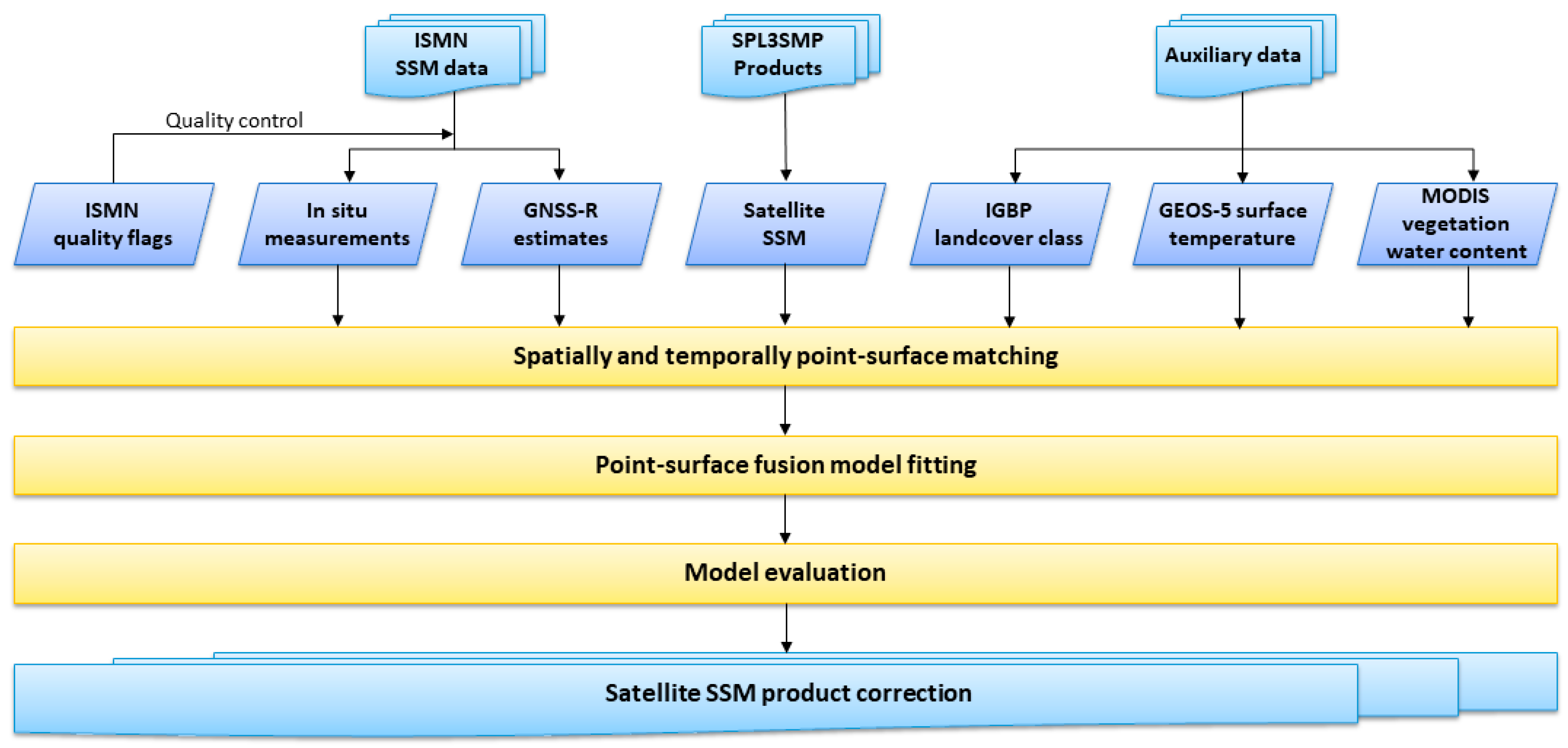
2.6. Data Pre-Processing

First, for both the in-situ and GNSS-R SSM data, the observations beyond their overlapping period with the SMAP SSM data ranging from 31 March 2015, to 31 August 2017, were excluded. In addition, according to the ISMN quality flags [34] that work as an indicator for the reliability of the data, only measurements flagged as “G” representing “good” quality were adopted for the in-situ and GNSS-R SSM data, and hence the high quality of the site-specific SSM time series was guaranteed.

Secondly, in order to account for the hourly recorded in-situ SSM data, the in-situ measurement closest in time and within a 3-h window of the SMAP 6 AM overpass for each day was used.

Finally, for the development of the fusion model, all the data sets needed to be matched spatially and temporally to obtain a coupled input–output training data pair, taking the SMAP SSM data as a reference. To be exact, the site-specific SSM data were associated with the pixels of the SMAP SSM data map as well as the three auxiliary data (LCC, SST, and VWC) maps covering the station. It should be noted that, although the GNSS-R sites have a sensing footprint of ~1000 m², this is insignificant compared to the scale of the SMAP SSM data (36-km EASEv2 grid). Furthermore, if a pixel had more than one corresponding site, then all the values for each station and for each day were averaged, i.e., one corresponding pixel of SMAP SSM coupled with only one averaged site-specific SSM time series. Eventually, we obtained 440 corresponding grid pixels. The data and pre-processing procedure are summarized in Figure 2.

Again, as mentioned in Section 2.2, we want to stress that no pre-processing was applied to the original SMAP SSM product due to the objective of our study being to improve the quality of all the available pixels.

3. Methodology

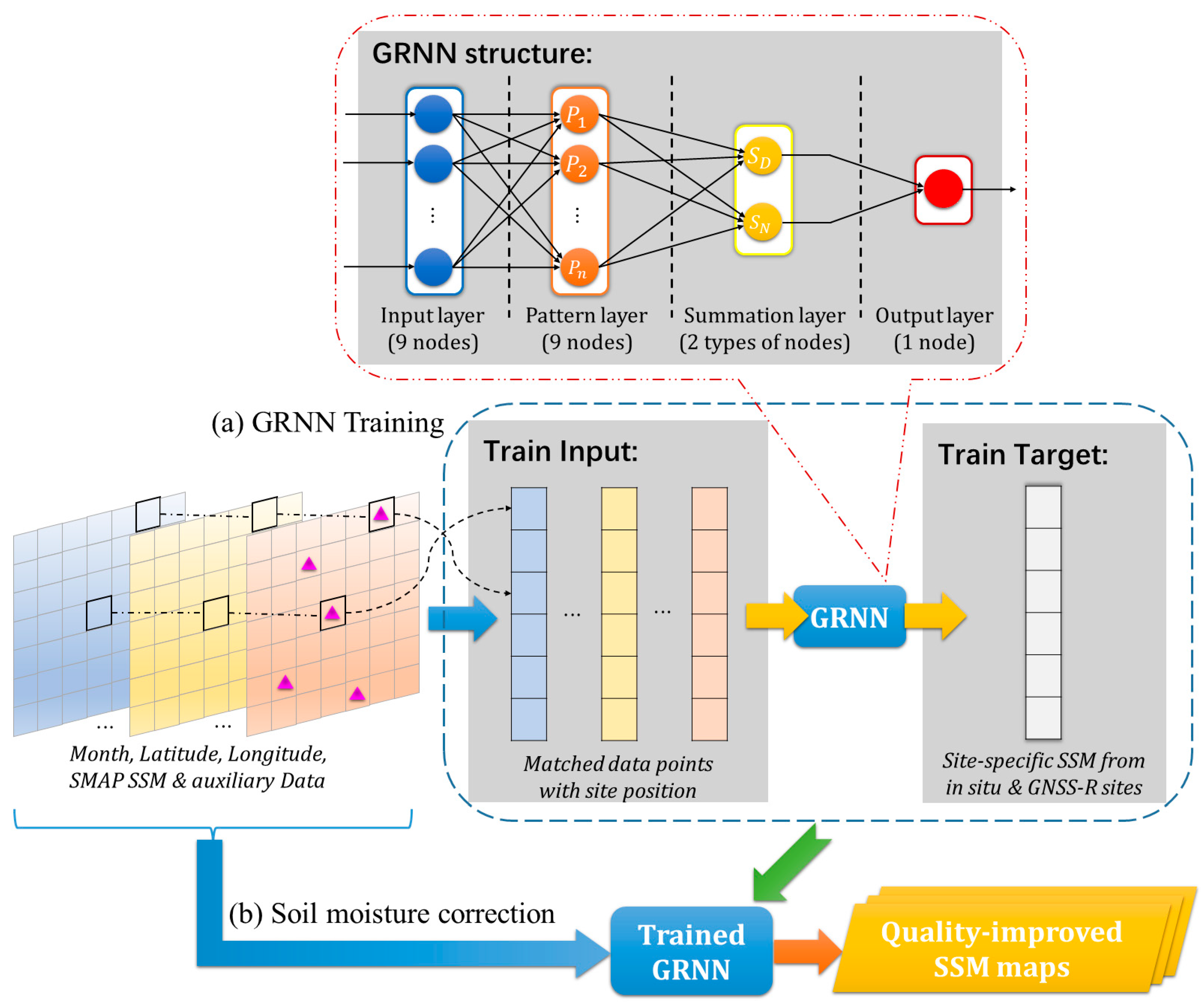
3.1. Generalized Regression Neural Network (GRNN) Model for SSM Quality Improvement

The entire flow of the point-surface fusion for satellite SSM quality improvement is illustrated in Figure 2. Considering that the satellite-derived SSM product and the site-specific SSM data are both affected by complicated factors, the relationship between them is generally non-linear. Consequently, we introduce the GRNN model [52,53] into our fusion scheme.

3.1.1. GRNN Model Structure

GRNN is a variation of the radial basis neural networks that is often used for function approximation [54]. A common GRNN consists of four layers: an input layer, a pattern layer, a summation layer, and an output layer (Figure 3). The pattern layer is fully connected with the input layer based on the radial basis function (RBF) kernel and owns the same amount of neurons as the input layer. The summation layer contains two types of summation neurons. One has only one neuron that sums up the estimates from the pattern neurons, while the other computes the weighted sum of the pattern neuron estimates weighted by the elements of the learning samples. After this, a dot function is performed by simply dividing the estimate of the second type of summation neuron by the first one to produce the output estimate.

The reasons for employing the GRNN model instead of other models lie in the following four aspects. Firstly, it is a relatively simple architecture with only two hidden layers, one pattern layer, and one summation layer. Meanwhile, the amount of neurons in the pattern layer is the same as the input layer, so there is no need to estimate the number of neurons in the hidden layers. Secondly, it is a single-pass learning method with no back-propagation required. Once the learning samples pass through the hidden layers, the training process of GRNN is accomplished. Therefore, the time cost and the computational expense of GRNN training are low. Thirdly, since GRNN is a variation of the radial basis neural networks based on the RBF kernel, it requires only one free parameter called the “spread” parameter. This parameter represents the width of the RBF kernel, and the larger the spread, the smoother the function approximation. It can be tuned by the cross-validation technique to an optimal value where the error reaches the minimum. Finally, unlike standard feedforward networks, GRNN estimation is always able to converge to a global solution and will not be trapped by a local minimum. That is to say, GRNN can serve our objective of improving the quality of the SSM product in the whole study area. In fact, the GRNN model has been successfully applied to generate regional-scale PM_2.5 over China from satellite-derived aerosol optical depth (AOD) products and ground-level fine particulate matter (PM_2.5, particulate matters with an aerodynamic diameter of 2.5 μm or less) measurements, and it performed much better than the conventional models (linear regression, multiple linear regression, and a semi-empirical model), as well as the more advanced models (geographically weighted regression and the back-propagation neural network (BPNN)) [55].

3.1.2. GRNN Model Fusion Procedure for SSM Quality Improvement

The procedure of the GRNN model for the point-surface SSM fusion is divided into two steps (Figure 3).

Step 1: GRNN training. The GRNN model was first trained on the coupled input–output training data pair (440 matched grid pixels, see Section 2.6) for the entire period (31 March 2015, to 31 August 2017). The SMAP SSM product combined with the LCC, SST, and VWC data was used as the input to the GRNN, while the site-specific (both in-situ and GNSS-R) SSM data were taken as the training targets. In addition, another three ancillary variables were also input into the GRNN model: the coincident month, the central latitude, and the central longitude of the SMAP 36-km EASEv2 grid pixels. Considering that the LCC data are actually a three-dimensional array, this resulted in a total of nine neurons for the input layers and only one neuron for the output layer of GRNN.

Step 2: Soil moisture correction. Once trained, the trained GRNN model was used to correct the original SMAP SSM data for the whole study area, and for each day, to produce quality-improved SSM maps.

The main function of GRNN is to determine the non-linear statistical relationship between the SMAP SSM and the relatively high quality site-specific SSM data. The LCC, SST, and VWC data containing the reflectivity, temperature, and vegetation information, respectively, were incorporated to account for their contribution to the retrieved SMAP SSM data. In particular, in order to allow for the temporal and spatial variation of soil moisture, the month, latitude, and longitude were also included. On the other hand, all the site-specific SSM data from both the in-situ and GNSS-R sites were taken as targets to enrich the quantity of sites and diversify the representativeness of the site-specific SSM. As for the “spread” parameter of GRNN, a value of 0.1 was set where the cross-validation RMSE was the minimum.

3.2. Conventional Methods for Comparison

In order to make a comprehensive assessment of the GRNN model employed in this study, another two classical regression analysis methods—multiple linear regression (MLR) and the Back-Propagation Neural Network (BPNN)—were selected for comparison, and underwent the same point-surface fusion process as GRNN.

The MLR is a classic statistical approach for modeling the relationship between a scalar dependent variable and more than one explanatory variable using the linear predictor functions. In this study, through incorporating auxiliary data related to SSM, it can be expressed as:

SSM_corr = β₀ + β₁ × SST + β₂ × VWC + β₃ × SSM_orig

(1)

where β₀ is the intercept for SM prediction and β₁–β₃ are regression coefficients for the predictor variables. SSM_orig and SSM_corr denote the original and MLR-corrected satellite SSM values, respectively.

The BPNN is the most commonly used multi-layer feedforward artificial neural network, which uses back-propagation as the training algorithm and has the potential to solve the multi-variable and nonlinear regression problems. In this study, a BPNN model with three layers (input layer, hidden layer, and output layer) was constructed. In order to be in agreement with the GRNN model, the input parameters of BPNN model were identical with those of the GRNN model. According to other works in the literature [56,57], the number of nodes in the hidden layer ranges from 2√n + μ to 2n + 1, where n and μ are the number of nodes in the input layer and output layer, respectively; therefore, in this study, the number of nodes in the hidden layer was varied from 7 to 19, and 18 nodes were found to constitute the lowest number of neurons that was able to derive the best performance (the minimum cross-validation RMSE), and were therefore selected in this paper.

3.3. Model Evaluation

The 10-fold cross-validation technique [58] was applied to test the model overfitting and predictive power. To start with, the dataset was first randomly divided into ten equal sized folds. Next, nine folds of the dataset were used as training data for fitting the model, and the remaining one fold was retained as the validation data for testing the model. Finally, we repeated this step a further nine times until every fold was tested. The ten results could then be averaged to produce a single estimation called the “cross-validation results”, whereas the model with the maximum correlation coefficient was selected as the best fitting model whose results are denoted as the “model fitting results”. It was then checked whether the model had been over-fitted, in which case the model performs drastically worse in the testing, i.e., the cross-validation results are much worse than the model fitting results.

The statistical metrics of the correlation coefficient (R, unit less), RMSE (cm³ cm⁻³), bias (cm³ cm⁻³), and unbiased RMSE (ubRMSE, cm³ cm⁻³) [59] were computed to quantify the level of agreement between the site-specific and satellite datasets, thereby providing an indication of the performance of the fusion model. The R describes of the temporal agreement between the datasets. It has a value between +1 and −1, where +1 is total positive linear correlation, 0 is no linear correlation, and −1 is total negative linear correlation. Absolute deviations between the site-specific and satellite data were expressed by the bias and the RMSE. Bias = 0 indicates an unbiased estimation, whereas bias <0 and bias >0 indicate underestimation and overestimation, respectively. RMSE is always non-negative, and a value of 0 (never achieved in practice) would indicate a perfect fit to the data. In general, a lower RMSE is better than a higher one. However, RMSE can be severely compromised if there are biases in the datasets. For this reason, the ubRMSE is also included to describe differences in data levels, which corrects for the mean biases, expressed as:

$${\mathrm{ubRMSE}}^2=\sqrt{{\mathrm{RMSE}}^2-{\mathrm{bias}}^2}$$

(2)

4. Results and Discussion

4.1. Assessment of the Model

4.1.1. Overall Performance of the Model

Table 2. Performance of the proposed GRNN model compared with MLR and BPNN.

Used SMAP SSM Values	Method	Model Fitting					Cross-Validation
		R	RMSE	bias	ub RMSE		R	RMSE	bias	ub RMSE
sm_sat-whole	MLR	0.50	0.086	0.000	0.086		0.50	0.086	0.000	0.086
	BPNN	0.76	0.065	0.000	0.065		0.75	0.066	0.000	0.065
	GRNN	0.90	0.045	0.001	0.044		0.87	0.050	0.001	0.050
sm_sat-rcmd	MLR	0.58	0.074	0.000	0.074		0.58	0.074	0.000	0.074
	BPNN	0.78	0.057	0.000	0.058		0.77	0.059	0.000	0.059
	GRNN	0.91	0.038	0.000	0.037		0.87	0.045	0.001	0.045

lists the model fitting and cross-validation results to evaluate the overall performance of the GRNN model, as well as the MLR model and BPNN model which underwent the same training and testing procedure as the GRNN using the 10-fold cross-validation technique for a fair comparison. Note the model fitting results are the results from the best fitting model, whereas the cross-validation results are the averaged results from the ten-round cross-validation. Besides, in order to allow a more realistic analysis between the SSM from the SMAP product and SSM from the fusion model, the experiments using only SMAP SSM values flagged as having the “recommended” retrieval quality were also carried out for comparison. For clarity, the original SMAP product including all SSM values denotes “sm_sat-whole”, whereas the quality controlled SMAP product including only “recommended” SSM values denotes “sm_sat-rcmd” hereinafter, i.e., the “sm_sat-whole” values consist of the “sm_sat-rcmd” values and those do not have the “recommended” retrieval quality.

In the model fitting, for “sm_sat-whole” (“sm_sat-rcmd”), the R values range from 0.50 (0.58) to 0.90 (0.91), and the ubRMSE values vary from 0.044 (0.037) to 0.086 (0.074) cm³ cm⁻³. In the cross-validation results, a similar trend can be seen. When comparing between the results using “sm_sat-whole” and “sm_sat-rcmd”, it can be found that the MLR model benefits a lot from using “sm_sat-rcmd”, the R value of which increased by 0.08 and ubRMSE decreased by 0.012 cm³ cm⁻³. The performances of the BPNN and GRNN models, however, improve a little using “sm_sat-rcmd”. This demonstrates that the non-linear regression method depends little on the quality of the input variables. In other words, the BPNN and GRNN model can correct the “non-recommended” SSM values in “sm_sat-whole” to obtain equivalent performances compared to that using “sm_sat-rcmd”.

Among the different methods, the MLR model performs the worst. There is a large improvement from the MLR model to the BPNN model, which makes sense because the relationship between SSM and input variables is generally non-linear and can be well constructed by the non-linear neural network. Moreover, the GRNN model outperforms the BPNN model, with further improvements in all the evaluation metrics. The superiority of the GRNN model compared to the BPNN model can be attributed to its high accuracy in the estimation, since it uses Gaussian functions, and the fact that it can handle noise in the inputs while converging rapidly. From the above, it can be suggested that the GRNN model is superior in assessing the non-linear relationship between the point- and surface-scale soil moisture datasets. Moreover, the fact that the cross-validated results are comparable to the model fitting results shows the GRNN model only results in slight overfitting.

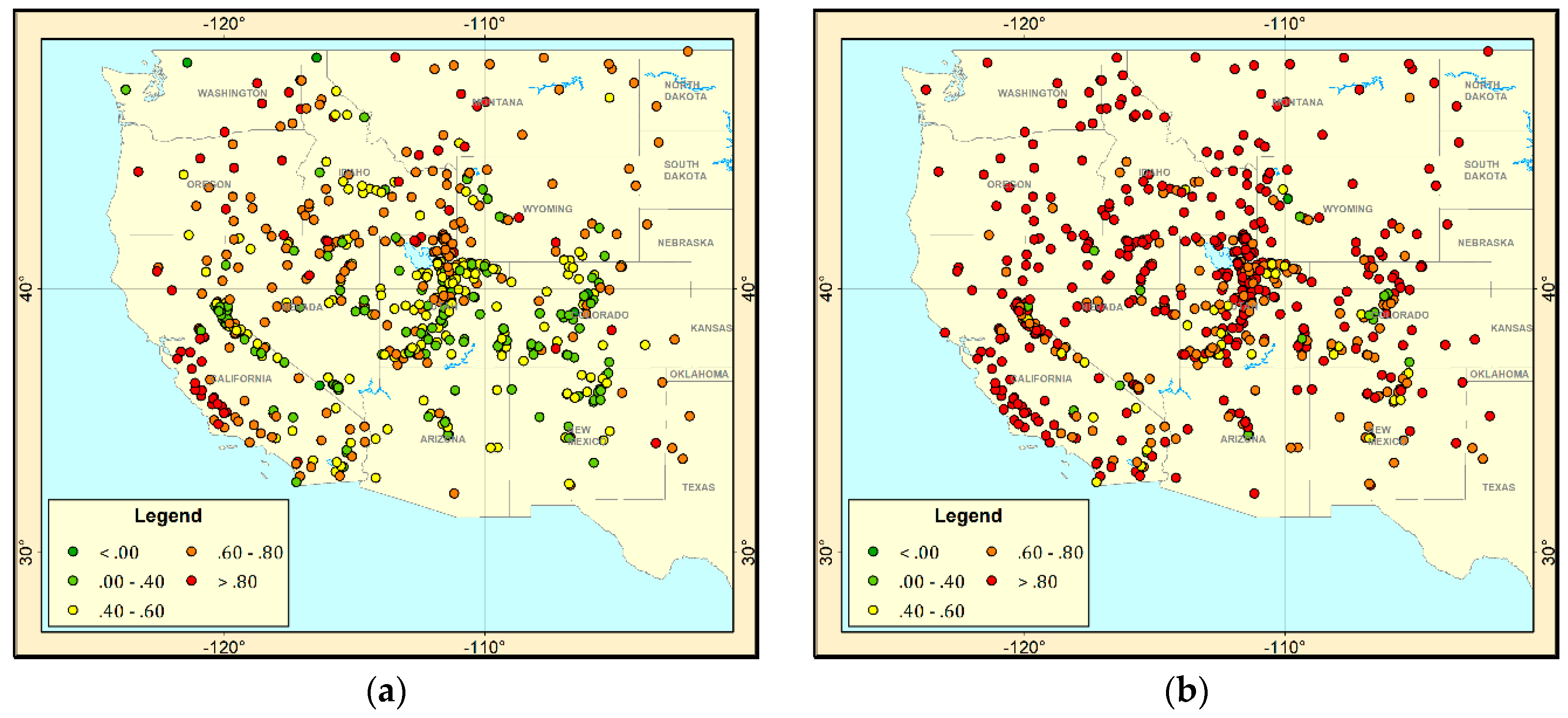
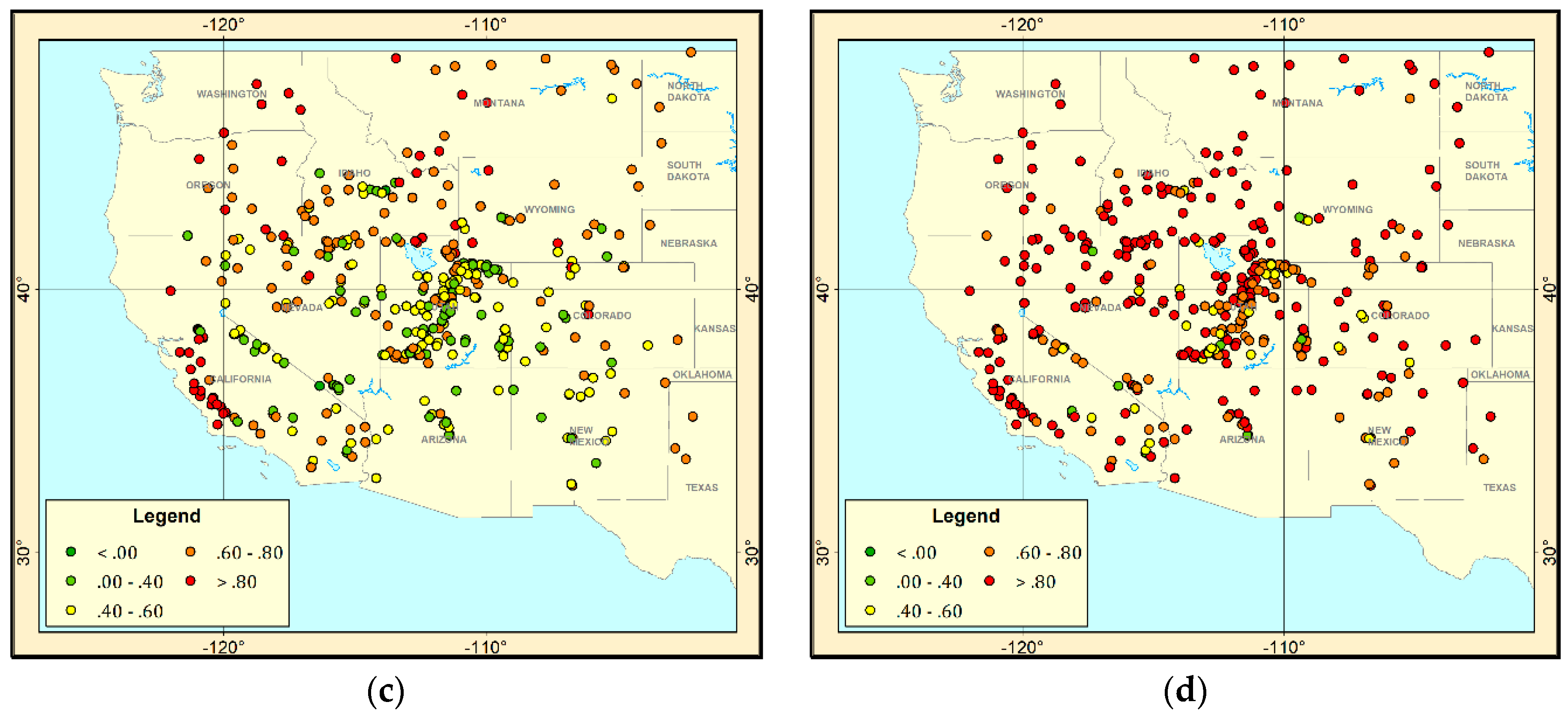
4.1.2. Model Performance for Each Station/Network

To make a further evaluation of the spatial performance of the GRNN model, the R values between the site-specific SSM with the matched pixel values of both the original (before fusion) and model-estimated (after fusion) SMAP SSM over each site were calculated, respectively, and are depicted in the form of a spatial distribution diagram (Figure 4). The same thing was done for the ubRMSE (Figure 5). For the reliability of calculated evaluation metrics at each site, a prior requirement of at least 30 coupled data points was set, thereby leaving 650 sites for “sm_sat-whole” to be considered. However, as for the “sm_sat-rcmd”, there were just 469 sites left, indicating that quite a number of “non-recommended” SSM values had been flagged out.

From Figure 4 and Figure 5, a general increase in R value and a decline in ubRMSE can be seen, with nearly all points for R becoming red (better) and nearly half the points for ubRMSE turning red (better) as well. According to the statistics, for “sm_sat-whole”, the number of sites with an R value greater than 0.6 is increased from 318 to 590, accounting for about 91% of the 650 sites, while the number of sites with ubRMSE values smaller than 0.04 cm³ cm⁻³ is tripled from 102 to 289 out of the total 650 stations under consideration. As for “sm_sat-rcmd”, the number of sites with an R value greater than 0.6 rises from 251 to 420, accounting for about 90% of the 469 sites, which is comparable to that for “sm_sat-whole”. Meanwhile, the number of sites with ubRMSE values smaller than 0.04 cm³ cm⁻³ is also largely increased from 106 to 264 out of the total 469 stations. Note that, due to the presence of the “non-recommended” SSM values in the “sm_sat-whole”, the “sm_sat-whole” values should have lower accuracy than the “sm_sat-rcmd” with respect to the site-specfic SSM data. This explains why the number of sites with ubRMSE values smaller than 0.04 cm³ cm⁻³ for “sm_sat-whole” is less than that for “sm_sat-rcmd” before fusion. However, this quantity becomes comparable after fusion, which demonstrates that the GRNN fusion model is able to correct the “non-recommended” SSM values from the satellite product.

As for spatial distribution, the higher R values before fusion (Figure 4a,c) are mainly clustered in the northern part and southwestern coast of the study area, where the form of the landscape in these regions is mainly plain terrain, while the lower R values are probably caused by the loss of accuracy of SMAP SSM retrieval due to the land surface environment being high mountain or desert. The same spatial distribution characteristic is apparent for ubRMSE as well (Figure 5a,c). Then, after fusion, the sites that previously had low R values or high ubRMSE values are much improved, and those whose R or ubRMSE values were already very good before fusion are further improved (compare Figure 4b,d with Figure 5b,d), respectively).

In addition, we calculated the average evaluation metrics both before and after fusion for each network (four in-situ networks and one GNSS-R network) to find out whether or not the point-surface synergy scheme works well on the different networks (

Table 3. Performance of the GRNN model on each network using “sm_sat-whole”.

Network	Before Fusion					After Fusion
	R	RMSE	bias	ub RMSE		R	RMSE	bias	ub RMSE
SCAN	0.57	0.076	−0.004	0.050		0.77	0.046	0.011	0.036
SNOTEL	0.50	0.129	−0.027	0.079		0.80	0.071	−0.004	0.053
SoilSCAPE	0.82	0.082	0.019	0.048		0.88	0.052	0.003	0.037
USCRN	0.67	0.101	0.033	0.050		0.87	0.033	0.003	0.029
PBO H2O	0.69	0.081	−0.006	0.053		0.82	0.042	0.002	0.038

). For simplicity, only the cross-validation results using “sm_sat-whole” are listed in the table. What needs to be stressed is that the mean R value of the SoilSCAPE network with respect to the original SMAP SSM is comparatively high (0.82 before fusion). This is because all 78 sites from the SoilSCAPE network correspond with only two pixels of the SMAP 36-km EASEv2 grid, resulting in its fairly good representativeness for the pixels.

From the table it can be noted that nearly all the mean evaluation metrics on each network experience large improvements after fusion. The mean R value of the SNOTEL network increases the most by 0.30, while its mean ubRMSE value decreases the most as well, from 0.079 to 0.053 cm³ cm⁻³. Furthermore, the mean ubRMSE values of all the networks except the SNOTEL network become less than 0.04 cm³ cm⁻³, thereby meeting the accuracy requirement of the SMAP mission. The unsatisfactory results for the SNOTEL network may be due to the fact that a number of sites in the SNOTEL network are concentrated along the mountain ranges, where the satellite soil moisture retrieval algorithm works poorly. From the metrics before fusion, we can also see that the relationship between the SNOTEL network and the original SMAP SSM is the worst of all, which may explain its environmental difficulty for the SMAP SSM retrieval algorithm. Another point to note is that because all the available pixel values of the SMAP SSM data, regardless of whether they had the “recommended” quality or not, were taken into consideration, as mentioned in Section 2.2, this would have exacerbated the results before fusion. On the other hand, it is undeniable that the results after fusion are much better than the original, and are close to the accuracy requirement of the SMAP mission.

4.2. Generation of the Quality-Improved SMAP SSM Product

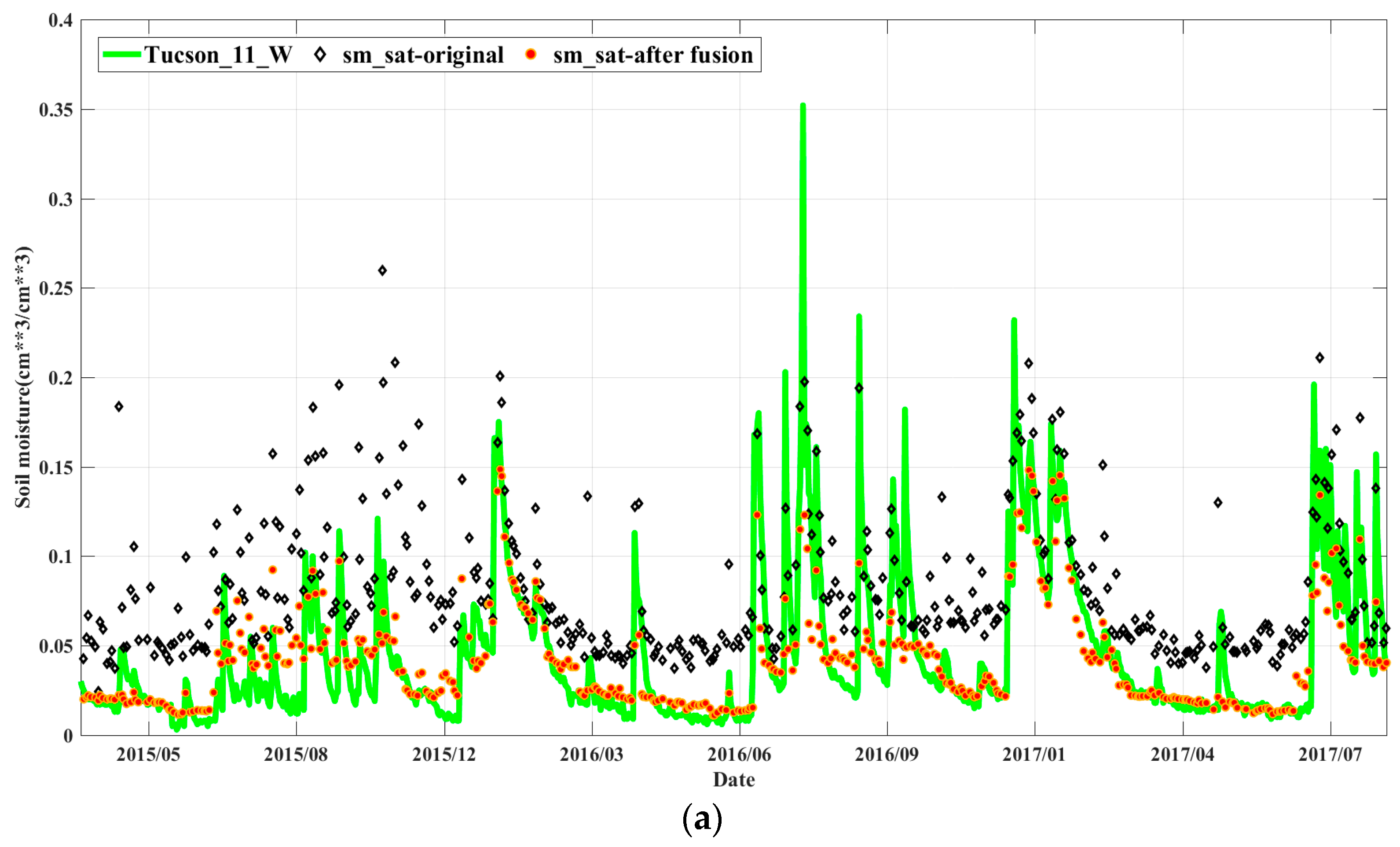
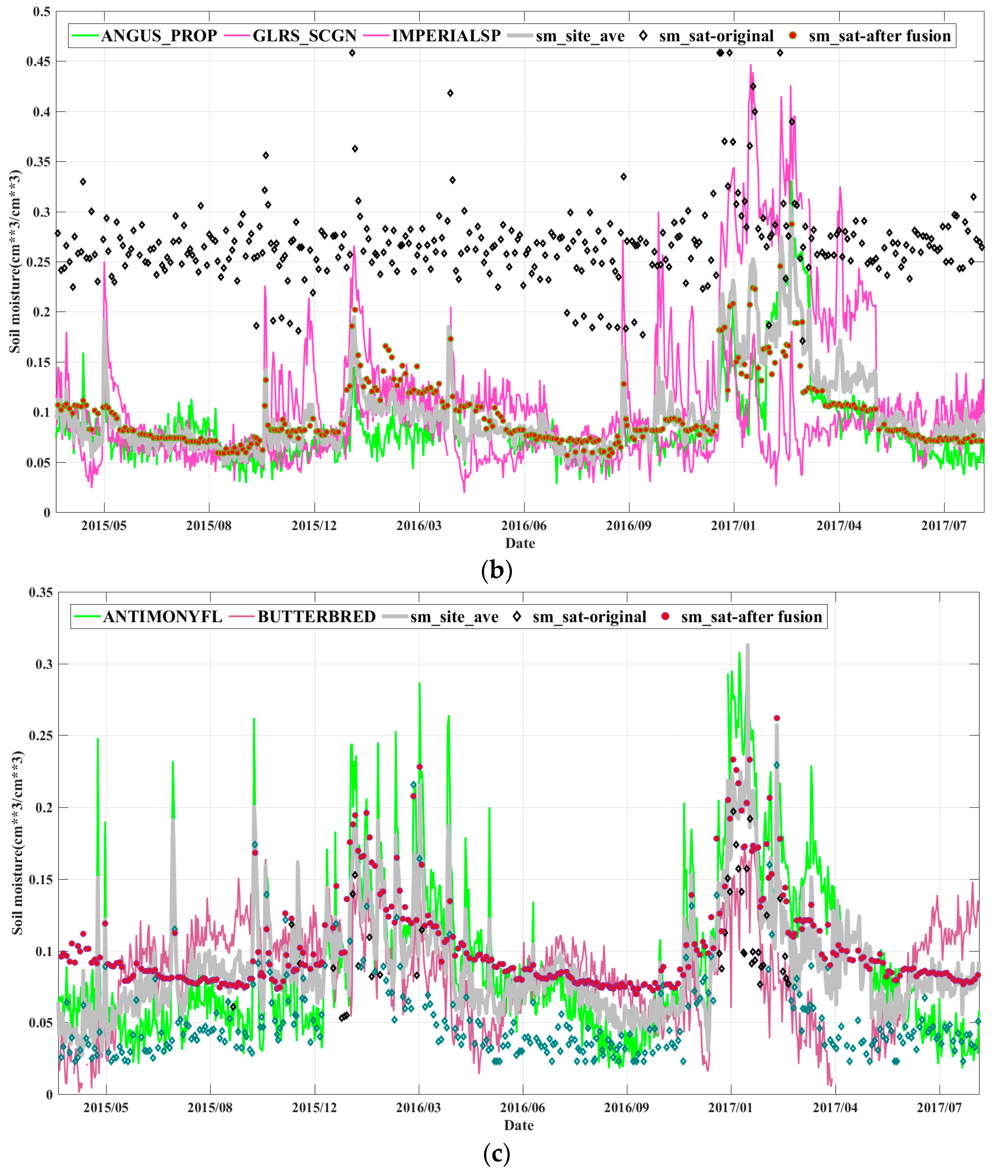
4.2.1. GRNN-Estimated SSM Time Series over Pixels

Based on the above results, which demonstrate that GRNN can be used to improve the quality of the SMAP SSM data, we applied the trained GRNN model to the original SMAP SSM product to produce quality-improved SSM maps. Before this, we compared the site-specific SSM time series with the coincident original, as well as the fused SMAP SSM time series for each pixel, in order to obtain an in-depth understanding of the temporal performance of the GRNN model. Figure 6 shows three examples of pixels. The SSM time series from ground sites within the pixel are drawn as lines. When one pixel of the SMAP EASEv2 grid includes more than one site, we use different colored-lines to indicate SSM values from different sites, and further use the average SSM from all the sites within the pixel (drawn as a wider line in gray color) to represent the site-specific SSM for the pixel. Besides, the sequences of black hollow diamonds and red solid circles denote the satellite SSM time series before and after fusion, respectively. Note that we use the dark cyan color to highlight the diamonds that have “recommended” SMAP SSM values. In other words, the black hollow diamonds actually represent the “non-recommended” SMAP SSM values.

The variations of the fused SSM (“sm_sat-after fusion”) over time are much more consistent with the site-specific SSM time series than the original (“sm_sat-original”), which means that the original SMAP SSM time series are well modified by the point-surface fusion process. In particular, outliers in the original SMAP SSM data are commendably corrected. For example, in Figure 6b the original SMAP SSM time series oscillate irregularly around the soil moisture value of 0.25 cm³ cm⁻³, which disagree significantly with the site-specific SSM variations; therefore, almost all of them are flagged as “non-recommended” values in the SMAP product. However, after applying the GRNN fusion model to these outlier values, they are well modified to approach the value of the site-specific SSM. Besides, the “recommended” SMAP SSM values in Figure 6c are also changed to be more consistent with the site-specific SSM time series. These results demonstrate that the proposed GRNN fusion model has the capacity to improve the quality of the whole satellite-derived SSM product, including both the “non-recommended” and “recommended” SSM values. Nevertheless, over- and under-estimates in the fused SSM time series do exist, which suggests the proposed fusion method needs further refinement. Moreover, the sharp rise in SSM data commonly following precipitation events can also be characterized by the fused SMAP SSM, to a certain degree.

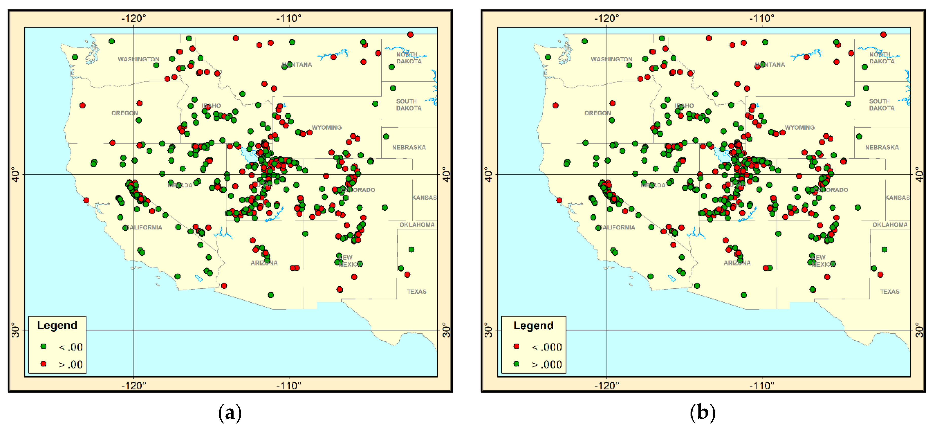
4.2.2. Mapping of the Quality-Improved SMAP SSM Product

Based on the established non-linear and non-localized relationship between the SMAP SSM and site-specific SSM, the original SMAP SSM product of the whole study area was then input into the trained GRNN model, and the outputs were generated as the quality-improved SSM maps of each day. For the sake of simplicity and clarity, we calculated the annual mean SSM map of the year 2016 both before and after fusion, respectively (Figure 7a,b). In addition, the annual mean SSM map from both the in-situ and GNSS-R sites was also calculated and is provided as a reference (Figure 7c).

As can be seen, the site-specific annual mean SSM values are more consistent with the fused annual mean SSM values than the original. Furthermore, the fused SSM map shows similar regional patterns to the topography, with higher soil moisture found along the rivers and plains and lower soil moisture concentrating around the deserts. In addition, the suspicious pixels neighboring the sea, where extremely high values exist in the original SMAP annual mean SSM map, are also well corrected.

4.3. Discussion

In this study, both in-situ and GNSS-R sites were used as targets for the GRNN model, which resulted in a satisfactory model performance and served our goal of improving the quality of the SMAP SSM product. However, it is important to note that the measurement scale of the GNSS-R technique (~1000 m²) is quite different from that of the in-situ measurements (<1 m²), which means that data inconsistency exists between the GNSS-R estimated and in-situ measured SSM. In addition, the temporal resolutions of these two SSM datasets are also different (daily for GNSS-R and hourly for in-situ), and the sampling time of GNSS-R SSM (at 12:00 UTC) is not coincident with that of SMAP SSM (at 6:00 a.m. local solar time) and the in-situ SSM data (closest in time and within a 3-h window of the SMAP 6:00 a.m. overpass) used in this study. This raises the question of whether the incorporation of the GNSS-R sites is beneficial for the GRNN training process. In order to answer this question, we undertook a separate comparison test.

We removed the GNSS-R SSM data of the PBO H2O network from the test and conducted the same point-surface fusion experiment using the GNSS-R model, as described in the previous sections, but for the SSM data from the in-situ sites only. Note that, we still used the same in-situ measurements that are closest in time and within a 3-h window of the SMAP 6 AM overpass for each day as previous sections did. We then calculated the difference between the R and ubRMSE values of the fusion results without the GNSS-R SSM data and the previous fusion results obtained with the GNSS-R SSM data for each in-situ site. The spatial distribution diagrams of R (Figure 8a) and ubRMSE (Figure 8b) are depicted in order to explore the consequences of the incorporation of the GNSS-R sites. Note that there were only 524 in-situ sites with available R and ubRMSE values out of the total 584 in-situ sites. In both Figure 8a,b, the red points indicate sites where the metrics (R or ubRMSE) improved after the addition of the GNSS-R sites, while the green points represent the sites where there was a decline.

In general, the sites that show positive R difference values are nearly identical in number to those that show negative ubRMSE difference values. The maximum increase in R value is 0.11, while the maximum decrease in ubRMSE value is 0.012 cm³ cm⁻³. However, less than half of the in-situ sites show an improvement after incorporating the GNSS-R network in the fusion scheme. The statistics indicate that the number of sites with a positive R difference is 205, and the number of sites with a negative ubRMSE difference is 195 out of the total 524 in-situ stations under consideration.

From the perspective of the spatial distribution, the stations that show an improvement are mainly concentrated around the regions where GNSS-R sites are distributed nearby, and there are more sites showing improvements in the areas with densely distributed in-situ stations. However, it should be noted that, in the southwest part of the study area, where there are quite a few GNSS-R sites along the coast, the R and ubRMSE values for the in-situ sites in this area have become worse. The main reason for this phenomenon may be the different resolutions of the two types of data. Not only that, but the land terrain fluctuation in this region may result in low-accuracy GNSS-R SSM estimates, which affect the subsequent training process. In conclusion, the results obtained in this study demonstrate that the incorporation of the GNSS-R sites plays a limited but non-negligible part in the point-surface fusion scheme.

Furthermore, an additional difficulty of using in-situ and GNSS-R measurements is the scale mismatch issue. Although the sensing footprint of the GNSS-R technique is field scale (~1000 m²), which is better than the typical point-scale (<1 m²) in-situ measurements, it is also different from the coarse-scale (tens of km²) of the microwave satellite observation. To date, various upscaling strategies have been developed to upscale point-scale soil moisture for the validation of coarse-resolution satellite soil moisture products as elaborated in Ref. [27]. Among them, the Triple Collocation (TC) [60], or Extended Triple Collocation (ETC) [61] method is deemed the most reliable. However, the ability of TC can be limited due to violations in the underlying assumptions [62], and it is just an evaluation method which cannot serve well the purpose of our study. Therefore, we decided to do the minimal effort by simply using the site-averaged soil moisture within each satellite pixel, and the results in the previous sections came out satisfactory for our goal in general. For many sites, the GRNN model manages to find a good non-linear mapping from SMAP SSM to the site-specific measurements. In contrast, there are sites for which the GRNN model does not provide a good estimation of the site-specific. Those in-situ sites are probably not representative of the satellite observation scale. Since our work is a preliminary study on the point-surface fusion of soil moisture using in-situ and GNSS-R measurements based on machine learning, there is still space for exploration in the future work. We will continue to work on this issue in the future.

What is more, an additional concern in this study is the use of time (month) and location (latitude and longitude) as input information into the proposed fusion model. Considering soil moisture is a highly temporal and spatial varying variable, it is very important to characterize its temporal and spatial variations since the main function of the model is to determine the non-linear statistical relationship between soil moisture data sets. To this end, we intended to use time and location to account for the seasonal variability and spatial heterogeneity of soil moisture. However, many other works using neural networks for soil moisture retrieval do not use time or location as input information (e.g., [63,64,65,66]). Therefore, to make a comprehensive analysis, we also conducted the same point-surface fusion experiments as in Section 4.1.1 but without time and location data (

Table 4. Performance of the fusion models without time and location input information.

Used SMAP SSM Values	Method	Model Fitting					Cross-Validation
		R	RMSE	bias	ub RMSE		R	RMSE	bias	ub RMSE
sm_sat-whole	MLR	-	-	-	-		-	-	-	-
	BPNN	0.67	0.074	0.000	0.074		0.67	0.074	0.000	0.074
	GRNN	0.69	0.072	0.001	0.071		0.69	0.073	0.001	0.073
sm_sat-rcmd	MLR	-	-	-	-		-	-	-	-
	BPNN	0.69	0.066	0.000	0.066		0.69	0.066	0.000	0.066
	GRNN	0.72	0.064	0.001	0.063		0.70	0.065	0.001	0.065

). Note that the MLR model itself does not include the time and location variables; therefore, the performance of MLR model (the same as in Table 2) is not shown.

Compared to the evaluation results that used time and location as input information (see Table 2), it can be seen from Table 4 that no matter whether for “sm_sat-whole” or “sm_sat-rcmd”, all the evaluation metrics of both the BPNN and GRNN models experience great deteriorations when the time and location data are excluded. For example, as for “sm_sat-whole”, the cross-validated R value decreased by 0.08 and 0.18 for the BPNN and GRNN models, respectively, whereas for “sm_sat-rcmd”, the cross-validated R value also decreased a lot by 0.08 and 0.17 for the BPNN and GRNN models, respectively. These results show that the performance of the fusion models indeed became promoted after incorporating the time and location data. In addition, it should be noticed that when using the time and location as input information, the GRNN model performs much better than the BPNN model (see Table 2), whereas after excluding the time and location data, the performance of the BPNN model becomes competitive to the GRNN model. This indicates that the time and location data play a much more important role in the proposed GRNN fusion model than in the BPNN model.

5. Conclusions and Future Work

This study innovatively introduced the GRNN method to improve the quality of the SMAP SSM product by fusing it with the site-specific SSM data from four in-situ networks and one GNSS-R network. The evaluation results obtained using a 10-fold cross-validation technique showed that the GRNN model outperformed the two other classical regression analysis methods (MLR and BPNN), with a cross-validation R value of approximately 0.9 and a ubRMSE value of 0.044 cm³ cm⁻³ using the whole SMAP product, which demonstrated that GRNN can accurately describe the non-linear and non-localized relationship between the site-specific SSM and SMAP SSM data. The further analysis of the spatio-temporal performance of the GRNN model indicated that the point-surface fusion approach has the capacity to provide reasonable information for improving the quality of the SMAP SSM product. Besides, the comparisons between the results using the whole SMAP product and the quality controlled SMAP product (only “recommended” SSM values) show that the proposed GRNN fusion model has the capacity to improve the quality of both “non-recommended” and “recommended” SSM values, which further suggests the added-value of our approach. Finally, quality-improved SSM maps were produced based on the trained GRNN model, and they showed spatial patterns consistent with the site-specific SSM values, as well as the topography of the land surface. The fusion test comparing the results obtained with and without the GNSS-R sites showed that the incorporation of the GNSS-R sites was beneficial for the synergy scheme, to a certain degree, and it was suggested that not only the in-situ sensors but also the GNSS-R equipment can be regarded as important soil moisture data sources in effective environmental monitoring.

Our future work with regard to the ideology proposed in this paper will focus on the following three aspects: First, because the proposed multi-source point-surface data fusion method is not just applicable to the SMAP mission, it could also serve to improve the quality of other satellite-derived soil moisture products. Therefore, other satellite missions such as SMOS and ASCAT will be considered in our experimental plan. Second, an in-depth investigation needs to be undertaken to explore the contribution of auxiliary data to the satellite-derived SSM data and to the GRNN model performance. Finally, in addition to the GRNN method used to construct the non-linear relationship between the SMAP SSM and the site-specific SSM data, employing a state-of-the-art deep learning technique in our synergy scheme may rival the performance of the GRNN model.

References

1. Mccoll, K.A.; Alemohammad, S.H.; Akbar, R.; Konings, A.G.; Yueh, S.; Entekhabi, D. The global distribution and dynamics of surface soil moisture. Nat. Geosci. 2017, 10, 100–104. [Google Scholar] [CrossRef]
2. Fischer, E.M.; Seneviratne, S.I.; Lüthi, D.; Schär, C. Contribution of land-atmosphere coupling to recent european summer heat waves. Geophys. Res. Lett. 2007, 34, 125–141. [Google Scholar] [CrossRef]
3. Trenberth, K.E. Evaluation of the global atmospheric moisture budget as seen from analyses. J. Clim. 1995, 8, 2255–2280. [Google Scholar] [CrossRef]
4. Viterbo, P.; Betts, A.K. Impact of the ECMWF reanalysis soil water on forecasts of the July 1993 Mississippi flood. J. Geophys. Res. Atmos. 1999, 104, 19361–19366. [Google Scholar] [CrossRef] [Green Version]
5. Litschi, M. Land-atmosphere coupling and climate change in europe. Nature 2006, 443, 205–209. [Google Scholar]
6. Seneviratne, S.I.; Corti, T.; Davin, E.L.; Hirschi, M.; Jaeger, E.B.; Lehner, I.; Orlowsky, B.; Teuling, A.J. Investigating soil moisture–climate interactions in a changing climate: A review. Earth Sci. Rev. 2010, 99, 125–161. [Google Scholar] [CrossRef]
7. Williams, C.A.; Albertson, J.D. Soil moisture controls on canopy-scale water and carbon fluxes in an African savanna. Water Resour. Res. 2004, 40, 333–341. [Google Scholar] [CrossRef]
8. Kurc, S.A.; Small, E.E. Soil moisture variations and ecosystem-scale fluxes of water and carbon in semiarid grassland and shrubland. Water Resour. Res. 2007, 43, 227–228. [Google Scholar] [CrossRef]
9. Rosenzweig, C.; Tubiello, F.N.; Goldberg, R.; Mills, E.; Bloomfield, J. Increased crop damage in the US from excess precipitation under climate change. Glob. Environ. Chang. 2002, 12, 197–202. [Google Scholar] [CrossRef] [Green Version]
10. Schmugge, T.; Gloersen, P.; Wilheit, T.; Geiger, F. Remote sensing of soil moisture with microwave radiometers. J. Geophys. Res. 1974, 79, 317–323. [Google Scholar] [CrossRef] [Green Version]
11. Entekhabi, D.; Njoku, E.G.; Neill, P.E.O.; Kellogg, K.H.; Crow, W.T.; Edelstein, W.N.; Entin, J.K.; Goodman, S.D.; Jackson, T.J.; Johnson, J. The soil moisture active passive (smap) mission. Proc. IEEE 2010, 98, 704–716. [Google Scholar] [CrossRef]
12. Kerr, Y.H.; Al-Yaari, A.; Rodriguez-Fernandez, N.; Parrens, M.; Molero, B.; Leroux, D.; Bircher, S.; Mahmoodi, A.; Mialon, A.; Richaume, P. Overview of smos performance in terms of global soil moisture monitoring after six years in operation. Remote Sens. Environ. 2016, 180, 40–63. [Google Scholar] [CrossRef]
13. Albergel, C.; Rosnay, P.D.; Gruhier, C.; Muñoz-Sabater, J.; Hasenauer, S.; Isaksen, L.; Kerr, Y.; Wagner, W. Evaluation of remotely sensed and modelled soil moisture products using global ground-based in situ observations. Remote Sens. Environ. 2012, 118, 215–226. [Google Scholar] [CrossRef]
14. Peng, J.; Niesel, J.; Loew, A.; Zhang, S.; Wang, J. Evaluation of satellite and reanalysis soil moisture products over southwest China using ground-based measurements. Remote Sens. 2015, 7, 15729–15747. [Google Scholar] [CrossRef]
15. Dorigo, W.A.; Gruber, A.; Jeu, R.A.M.D.; Wagner, W.; Stacke, T.; Loew, A.; Albergel, C.; Brocca, L.; Chung, D.; Parinussa, R.M. Evaluation of the esa cci soil moisture product using ground-based observations. Remote Sens. Environ. 2015, 162, 380–395. [Google Scholar] [CrossRef]
16. Jackson, T.J.; Bindlish, R.; Cosh, M.H.; Zhao, T.; Starks, P.J.; Bosch, D.D.; Seyfried, M.; Moran, M.S.; Goodrich, D.C.; Kerr, Y.H. Validation of soil moisture and ocean salinity (SMOS) soil moisture over watershed networks in the U.S. IEEE Trans. Geosci. Remote Sens. 2012, 50, 1530–1543. [Google Scholar] [CrossRef] [Green Version]
17. Sanchez, N.; Martinez-Fernandez, J.; Scaini, A.; Perez-Gutierrez, C. Validation of the SMOS L2 soil moisture data in the REMEDHUS network (Spain). IEEE Trans. Geosci. Remote Sens. 2012, 50, 1602–1611. [Google Scholar] [CrossRef]
18. Li, Y.; Grimaldi, S.; Walker, J.P.; Pauwels, V.R.N. Application of remote sensing data to constrain operational rainfall-driven flood forecasting: A review. Remote Sens. 2016, 8, 456. [Google Scholar] [CrossRef]
19. Loew, A.; Stacke, T.; Dorigo, W.; Jeu, R.D. Potential and limitations of multidecadal satellite soil moisture observations for climate model evaluation studies. Hydrol. Earth Syst. Sci. 2013, 17, 3523–3542. [Google Scholar] [CrossRef]
20. Aghakouchak, A.; Farahmand, A.; Melton, F.S.; Teixeira, J.; Anderson, M.C.; Wardlow, B.D.; Hain, C.R. Remote sensing of drought: Progress, challenges and opportunities. Rev. Geophys. 2015, 53, 452–480. [Google Scholar] [CrossRef] [Green Version]
21. Brocca, L.; Crow, W.T.; Ciabatta, L.; Massari, C.; Rosnay, P.D.; Enenkel, M.; Hahn, S.; Amarnath, G.; Camici, S.; Tarpanelli, A. A review of the applications of ascat soil moisture products. IEEE J. Sel. Top. Appl. Earth Obs. Remote Sens. 2017, 10, 2285–2306. [Google Scholar] [CrossRef]
22. Mohanty, B.P.; Cosh, M.; Lakshmi, V.; Montzka, C. Remote sensing for vadose zone hydrology—A synthesis from the vantage point. Vadose Zone J. 2013, 12, 155–175. [Google Scholar] [CrossRef]
23. Burgin, M.S.; Colliander, A.; Njoku, E.G.; Chan, S.K.; Cabot, F.; Kerr, Y.H.; Bindlish, R.; Jackson, T.J.; Entekhabi, D.; Yueh, S.H. A comparative study of the smap passive soil moisture product with existing satellite-based soil moisture products. IEEE Trans. Geosci. Remote Sens. 2017, 55, 2959–2971. [Google Scholar] [CrossRef]
24. Entekhabi, D.; Yueh, S.; O’Neill, P.; Kellogg, K.; Allen, A.; Bindlish, R.; Brown, M.; Chan, S.; Colliander, A.; Crow, W. Smap Handbook; JPL Publication JPL 400-1567; Jet Propulsion Laboratory: Pasadena, CA, USA, 2014; p. 182.
25. Kerr, Y.; Waldteufel, P.; Richaume, P.; Davenport, I.; Ferrazzoli, P.; Wigneron, J. Smos Level 2 Processor Soil Moisture Algorithm Theoretical Basis Document (atbd). In sm-esl (cbsa), Toulouse. Array Systems Computing Inc.: Toronto, ON, Canada, 2015. Available online: https://earth.esa.int/documents/10174/1854519/SMOS_L2_SM_ATBD (accessed on 20 June 2018).
26. Ochsner, T.E.; Cosh, M.H.; Cuenca, R.H.; Dorigo, W.A.; Draper, C.S.; Hagimoto, Y.; Kerr, Y.H.; Njoku, E.G.; Small, E.E.; Zreda, M. State of the art in large-scale soil moisture monitoring. Soil Sci. Soc. Am. J. 2013, 77, 1888–1919. [Google Scholar] [CrossRef] [Green Version]
27. Crow, W.T.; Berg, A.A.; Cosh, M.H.; Loew, A.; Mohanty, B.P.; Panciera, R.; Rosnay, P.; Ryu, D.; Walker, J.P. Upscaling sparse ground-based soil moisture observations for the validation of coarse-resolution satellite soil moisture products. Rev. Geophys. 2012, 50. [Google Scholar] [CrossRef] [Green Version]
28. Larson, K.M. Gps interferometric reflectometry: Applications to surface soil moisture, snow depth, and vegetation water content in the western United States. Wiley Interdiscip. Rev. Water 2016, 3, 775–787. [Google Scholar] [CrossRef]
29. Vey, S.; Güntner, A.; Wickert, J.; Blume, T.; Ramatschi, M. Long-term soil moisture dynamics derived from gnss interferometric reflectometry: A case study for sutherland, South Africa. GPS Solut. 2016, 20, 641–654. [Google Scholar] [CrossRef]
30. Small, E.E.; Larson, K.M.; Chew, C.C.; Dong, J.; Ochsner, T.E. Validation of gps-ir soil moisture retrievals: Comparison of different algorithms to remove vegetation effects. IEEE J. Sel. Top. Appl. Earth Obs. Remote Sens. 2016, 9, 4759–4770. [Google Scholar] [CrossRef]
31. Jackson, T.; Colliander, A.; Kimball, J.; Reichle, R.; Crow, W.; Entekhabi, D.; O’Neill, P.; Njoku, E. Soil Moisture Active Passive (Smap) Mission: Science Data Calibration and Validation Plan; jpl d-52544; Nasa Jet Propulsion Lab.: Pasadena, CA, USA, 2012; 99p.
32. Larson, K.M.; Small, E.E.; Gutmann, E.D.; Bilich, A.L.; Braun, J.J.; Zavorotny, V.U. Use of gps receivers as a soil moisture network for water cycle studies. Geophys. Res. Lett. 2008, 35. [Google Scholar] [CrossRef]
33. Dorigo, W.A.; Wagner, W.; Hohensinn, R.; Hahn, S.; Paulik, C.; Xaver, A.; Gruber, A.; Drusch, M.; Mecklenburg, S.; Oevelen, P.V. The international soil moisture network: A data hosting facility for global in situ soil moisture measurements. Hydrol. Earth Syst. Sci. 2011, 15, 1675–1698. [Google Scholar] [CrossRef]
34. Dorigo, W.A.; Xaver, A.; Vreugdenhil, M.; Gruber, A.; Hegyiová, A.; Sanchis-Dufau, A.D.; Zamojski, D.; Cordes, C.; Wagner, W.; Drusch, M. Global automated quality control of in situ soil moisture data from the international soil moisture network. Vadose Zone J. 2013, 12, 918–924. [Google Scholar] [CrossRef]
35. Zhang, X.; Chen, N. Reconstruction of gf-1 soil moisture observation based on satellite and in situ sensor collaboration under full cloud contamination. IEEE Trans. Geosci. Remote Sens. 2016, 54, 5185–5202. [Google Scholar] [CrossRef]
36. Xing, C.; Chen, N.; Zhang, X.; Gong, J. A machine learning based reconstruction method for satellite remote sensing of soil moisture images with in situ observations. Remote Sens. 2017, 9, 484. [Google Scholar] [CrossRef]
37. Rodríguez-Fernández, N.J.; de Souza, V.; Kerr, Y.H.; Richaume, P.; Al Bitar, A. Soil moisture retrieval using smos brightness temperatures and a neural network trained on in situ measurements. In Proceedings of the 2017 IEEE International Geoscience and Remote Sensing Symposium (IGARSS), Fort Worth, TX, USA, 23–28 July 2017; pp. 1574–1577. [Google Scholar]
38. O’Neill, P.; Chan, S.; Njoku, E.; Jackson, T.; Bindlish, R. Smap l3 radiometer global daily 36 km ease-grid soil moisture. Version 2016, 4, R14010. [Google Scholar]
39. O’Neill, P.; Njoku, E.; Jackson, T.; Chan, S.; Bindlish, R. Smap Algorithm Theoretical Basis Document: Level 2 & 3 Soil Moisture (Passive) Data Products; JPL D-66480 2015; Jet Propulsion Lab., California Inst. Technol.: Pasadena, CA, USA, 2012. Available online: http://nsidc.org/sites/nsidc.org/files/files/data/smap/pdfs/l2%263_sm_p_v4_oct2012.pdf (accessed on 20 June 2018).
40. Colliander, A.; Jackson, T.J.; Bindlish, R.; Chan, S.; Das, N.; Kim, S.B.; Cosh, M.H.; Dunbar, R.S.; Dang, L.; Pashaian, L. Validation of smap surface soil moisture products with core validation sites. Remote Sens. Environ. 2017, 191, 215–231. [Google Scholar] [CrossRef]
41. Schaefer, G.L.; Cosh, M.H.; Jackson, T.J. The USDA natural resources conservation service soil climate analysis network (SCAN). J. Atmos. Ocean. Technol. 2007, 24, 2073. [Google Scholar] [CrossRef]
42. Leavesley, G.H.; David, O.; Garen, D.C.; Lea, J.; Marron, J.K.; Pagano, T.C.; Perkins, T.R.; Strobel, M.L. A Modeling Framework for Improved Agricultural Water Supply Forecasting. In Proceedings of the AGU Fall Meeting Abstracts, 2008 Fall Meeting, San Francisco, CA, USA, 15–19 December 2008. [Google Scholar]
43. Moghaddam, M.; Entekhabi, D.; Goykhman, Y.; Li, K.; Liu, M.; Mahajan, A.; Nayyar, A.; Shuman, D.; Teneketzis, D. A wireless soil moisture smart sensor web using physics-based optimal control: Concept and initial demonstrations. IEEE J. Sel. Top. Appl. Earth Obs. Remote Sens. 2010, 3, 522–535. [Google Scholar] [CrossRef]
44. Moghaddam, M.; Silva, A.; Clewley, D.; Akbar, R.; Hussaini, S.; Whitcomb, J.; Devarakonda, R.; Shrestha, R.; Cook, R.; Prakash, G. Soil Moisture Profiles and Temperature Data from Soilscape Sites, USA; Ornl DAAC: Oak Ridge, TN, USA, 2016.
45. Bell, J.E.; Palecki, M.A.; Baker, C.B.; Collins, W.G.; Lawrimore, J.H.; Leeper, R.D.; Hall, M.E.; Kochendorfer, J.; Meyers, T.P.; Wilson, T.U.S. Climate reference network soil moisture and temperature observations. J. Hydrometeorol. 2013, 14, 977–988. [Google Scholar] [CrossRef]
46. Larson, K.M.; Braun, J.J.; Small, E.E.; Zavorotny, V.U.; Gutmann, E.D.; Bilich, A.L. Gps multipath and its relation to near-surface soil moisture content. IEEE J. Sel. Top. Appl. Earth Obs. Remote Sens. 2010, 3, 91–99. [Google Scholar] [CrossRef]
47. Larson, K.M.; Small, E.E.; Gutmann, E.; Bilich, A.; Axelrad, P.; Braun, J. Using GPS multipath to measure soil moisture fluctuations: Initial results. GPS Solut. 2008, 12, 173–177. [Google Scholar] [CrossRef]
48. Belward, A.S. The IGBP-DIS global 1-km land-cover data set DIS-cover: A project overview. Photogramm. Eng. Remote Sens. 1999, 65, 1013–1020. [Google Scholar]
49. Koster, R.D.; Suarez, M.J.; Ducharne, A.; Stieglitz, M.; Kumar, P. A catchment-based approach to modeling land surface processes in a general circulation model: 1. Model structure. J. Geophys. Res. Atmos. 2000, 105, 24809–24822. [Google Scholar] [CrossRef] [Green Version]
50. Ducharne, A.; Koster, R.D.; Suarez, M.J.; Stieglitz, M.; Kumar, P. A catchment-based approach to modeling land surface processes in a general circulation model: 2. Parameter estimation and model demonstration. J. Geophys. Res. Atmos. 2000, 105, 24823–24838. [Google Scholar] [CrossRef] [Green Version]
51. Wigneron, J.-P.; Chanzy, A.; Calvet, J.-C.; Bruguier, N. A simple algorithm to retrieve soil moisture and vegetation biomass using passive microwave measurements over crop fields. Remote Sens. Environ. 1995, 51, 331–341. [Google Scholar] [CrossRef]
52. Specht, D.F. A general regression neural network. IEEE Trans. Neural Netw. 1991, 2, 568–576. [Google Scholar] [CrossRef] [PubMed]
53. Specht, D.F. The general regression neural network-rediscovered. Neural Netw. 1993, 6, 1033–1034. [Google Scholar] [CrossRef]
54. Cheng, B.; Titterington, D.M. Neural networks: A review from a statistical perspective. Stat. Sci. 1994, 9, 2–30. [Google Scholar] [CrossRef]
55. Li, T.; Shen, H.; Zeng, C.; Yuan, Q.; Zhang, L. Point-surface fusion of station measurements and satellite observations for mapping PM2.5 distribution in China: Methods and assessment. Atmos. Environ. 2017, 152, 477–489. [Google Scholar] [CrossRef]
56. Reich, S.L.; Gomez, D.; Dawidowski, L. Artificial neural network for the identification of unknown air pollution sources. Atmos. Environ. 1999, 33, 3045–3052. [Google Scholar] [CrossRef]
57. Gardner, M.W.; Dorling, S. Artificial neural networks (the multilayer perceptron)—A review of applications in the atmospheric sciences. Atmos. Environ. 1998, 32, 2627–2636. [Google Scholar] [CrossRef]
58. Rodriguez, J.D.; Perez, A.; Lozano, J.A. Sensitivity analysis of k-fold cross validation in prediction error estimation. IEEE Trans. Pattern Anal. Mach. Intell. 2010, 32, 569–575. [Google Scholar] [CrossRef] [PubMed]
59. Entekhabi, D.; Reichle, R.H.; Koster, R.D.; Crow, W.T. Performance metrics for soil moisture retrievals and application requirements. J. Hydrometeorol. 2010, 11, 832–840. [Google Scholar] [CrossRef]
60. Stoffelen, A. Toward the true near-surface wind speed: Error modeling and calibration using triple collocation. J. Geophys. Res. Oceans 1998, 103, 7755–7766. [Google Scholar] [CrossRef] [Green Version]
61. McColl, K.A.; Vogelzang, J.; Konings, A.G.; Entekhabi, D.; Piles, M.; Stoffelen, A. Extended triple collocation: Estimating errors and correlation coefficients with respect to an unknown target. Geophys. Res. Lett. 2014, 41, 6229–6236. [Google Scholar] [CrossRef] [Green Version]
62. Gruber, A.; Su, C.-H.; Zwieback, S.; Crow, W.; Dorigo, W.; Wagner, W. Recent advances in (soil moisture) triple collocation analysis. Int. J. Appl. Earth Obs. Geoinf. 2016, 45, 200–211. [Google Scholar] [CrossRef]
63. Aires, F.; Prigent, C.; Rossow, W. Sensitivity of satellite microwave and infrared observations to soil moisture at a global scale: 2. Global statistical relationships. J. Geophys. Res. Atmos. 2005, 110. [Google Scholar] [CrossRef] [Green Version]
64. Kolassa, J.; Gentine, P.; Prigent, C.; Aires, F. Soil moisture retrieval from AMSR-E and ASCAT microwave observation synergy. Part 1: Satellite data analysis. Remote Sens. Environ. 2016, 173, 1–14. [Google Scholar] [CrossRef]
65. Pan, X.; Kornelsen, K.C.; Coulibaly, P. Estimating root zone soil moisture at continental scale using neural networks. JAWRA J. Am. Water Resour. Assoc. 2017, 53, 220–237. [Google Scholar] [CrossRef]
66. Alemohammad, S.H.; Kolassa, J.; Prigent, C.; Aires, F.; Gentine, P. Global downscaling of remotely-sensed soil moisture using neural networks. Hydrol. Earth Syst. Sci. 2018. under review. [Google Scholar] [CrossRef]
Figure 1. Study area (red rectangle, 32°N–49°N, 125°W–102°W) and distribution of the soil moisture networks including four in-situ networks (the Soil Climate Analysis Network (SCAN) network, the SNOwpack TELemetry (SNOTEL) network, the Soil moisture Sensing Controller and oPtimal Estimator (SoilSCAPE) network, and the U.S. Climate Reference Network (USCRN) network) and one Global Navigation Satellite System interferometric Reflectometry (GNSS-R) network (the PBO H2O network).
Remotesensing 10 01351 g001
Figure 2. Data and flow chart of point-surface fusion scheme for satellite SSM quality improvement.
Remotesensing 10 01351 g002
Figure 3. Schematic of the GRNN model used for SSM improvement and the two steps of the GRNN fusion approach: (a) GRNN training; and (b) soil moisture correction using the trained network.
Remotesensing 10 01351 g003
Figure 4. Spatial distribution of R between the site-specific SSM and original (a,c) and fused (b,d) SMAP SSM over each station using “sm_sat-whole” (a,b) and “sm_sat-rcmd” (c,d).
Remotesensing 10 01351 g004aRemotesensing 10 01351 g004b
Figure 5. Spatial distribution of ubRMSE between the site-specific SSM and original (a,c) and fused (b,d) SMAP SSM over each station using “sm_sat-whole” (a,b) and “sm_sat-rcmd” (c,d).
Remotesensing 10 01351 g005
Figure 6. Site-specific SSM time series compared with the coincident SMAP SSM time series before and after fusion for three examples of 36-km EASEv2 pixels, which include (a) one site (Tucson_11_W), (b) three sites (ANGUS_PROP, GLRS_SCGN, IMPERIALSP), and (c) two sites (ANTIMONYFL, BUTTERBRED), respectively. The central latitude and longitude of each pixel are (a) (32.2881°N, 111.0996°W), (b) (33.2921°N, 115.5809°W), and (c) (35.3352°N, 118.1950°W), respectively. Note that the dark cyan hollow diamonds denote “recommended” SSM values from SMAP product whereas the black hollow diamonds denote “non-recommended” SMAP SSM values.
Remotesensing 10 01351 g006aRemotesensing 10 01351 g006b
Figure 7. Annual mean SSM map of the year 2016 for (a) the original SMAP SSM, (b) the GRNN-estimated SSM, and (c) the site-specific SSM.
Remotesensing 10 01351 g007
Figure 8. Spatial distribution of the difference values of (a) R and (b) ubRMSE between the fusion results with and without the GNSS-R SSM data (the former minus the latter) over each in-situ site.
Remotesensing 10 01351 g008