Hyperspectral Image Classification Based on Parameter-Optimized 3D-CNNs Combined with Transfer Learning and Virtual Samples

Abstract

Recent research has shown that spatial-spectral information can help to improve the classification of hyperspectral images (HSIs). Therefore, three-dimensional convolutional neural networks (3D-CNNs) have been applied to HSI classification. However, a lack of HSI training samples restricts the performance of 3D-CNNs. To solve this problem and improve the classification, an improved method based on 3D-CNNs combined with parameter optimization, transfer learning, and virtual samples is proposed in this paper. Firstly, to optimize the network performance, the parameters of the 3D-CNN of the HSI to be classified (target data) are adjusted according to the single variable principle. Secondly, in order to relieve the problem caused by insufficient samples, the weights in the bottom layers of the parameter-optimized 3D-CNN of the target data can be transferred from another well trained 3D-CNN by a HSI (source data) with enough samples and the same feature space as the target data. Then, some virtual samples can be generated from the original samples of the target data to further alleviate the lack of HSI training samples. Finally, the parameter-optimized 3D-CNN with transfer learning can be trained by the training samples consisting of the virtual and the original samples. Experimental results on real-world hyperspectral satellite images have shown that the proposed method has great potential prospects in HSI classification.

1. Introduction

Hyperspectral images (HSIs) containing hundreds of spectral channels [1,2] can be represented as three-dimensional (3D) tensors [3,4] and have been investigated in many applications [5], for example agriculture [6,7], resource management [8,9], environmental monitoring [10,11,12] and so on. Land cover classification is one of the significant methods of mining information from HSIs and feature extraction is an important step in classification [13]. However, most of the traditional methods extract handcrafted features from HSIs in a shallow manner [14]. Therefore, effective feature extraction is one of the key factors to improve HSI classification [15,16,17,18].

Recently, as an important branch of machine learning [19,20,21,22,23], deep learning has attracted much interest due to its strong capabilities in analysis and feature extraction [24,25]. By extracting features of the input data from the bottom to the top of the network, deep-learning models can form the high-level abstract features suitable for pattern classification [26]. Among numerous deep-learning models, a convolutional neural network (CNN) has a relatively small number of weights owing to local connections and sharing weights [27]. Moreover, the multidimensional tensor data, for instance HSIs, can be directly input into 3D convolutional neural networks (3D-CNNs), which helps to preserve the original relevant information of the data and avoids complex data reconstruction [28,29,30]. Therefore, 3D-CNNs have been introduced to extract high-level invariant features and improve the classification performance of HSIs [31,32,33].

Sufficient training samples guarantee the performance of the deep model; however, labeled samples in HSIs are always limited [34,35,36,37]. Some representative methods, for example transfer learning [38,39], virtual samples [32], manifold regularization based on semi-supervised leaning [35,36,37], and so on, can help to solve the problem of limited samples [40,41,42]. The former two methods are suited for HSI data structures, the latter being more suitable for ordinary images. We assume that there is another HSI (source data) which has enough samples and the same feature space as the HSI to be classified (target data). Then, knowledge transfer can be made from the source data to the target domain to improve the network performance by avoiding rather expensive data labeling efforts [43]. If the source data is absent, as a pseudo-sample transformed from the original sample of the target data, virtual samples are also a solution to make up for the lack of HSI samples [44].

In addition, the network performance of 3D-CNNs can be influenced by the parameter settings. Therefore, in this paper, to solve the problem of insufficient samples and to further improve the classification of HSIs, a parameter-optimized 3D-CNN combined with transfer learning and virtual samples (named the PO-3DCNN-TV method hereinafter) is proposed. Firstly, a 3D-CNN of the target data could be built and its parameters adjusted according to the single variable principle. Secondly, to improve the network computing efficiency and to alleviate the problem of a lack of samples, transfer learning is introduced to the network and the weights in the bottom layers of the parameter-optimized 3D-CNN of the target data can be transferred from another well trained 3D-CNN by the source data. Then, the technology of virtual samples can be applied to further solve the problem of inadequate HSI samples. Finally, the 3D-CNN with optimized parameters and transferred weights can be trained by the training samples, mixing the virtual samples with the original samples in the target data.

The remainder of this paper is organized as follows: the three-dimensional convolutional neural network is introduced in Section 2; Section 3 presents a detailed description of the proposed classification method; some experimental results are discussed in Section 4; and Section 5 concludes this paper.

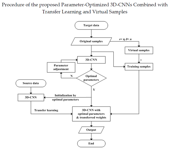
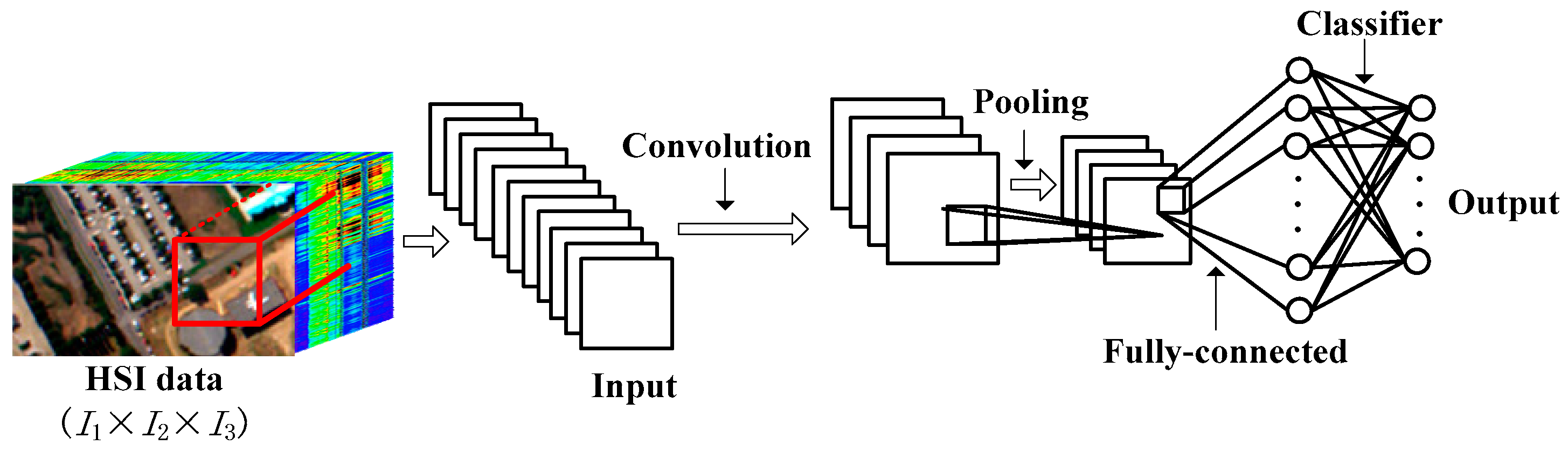
2. Overview of Three-Dimensional Convolutional Neural Networks

CNN is one of the most efficient methods of big data classification. Two-dimensional (2D) CNNs mainly capture features from the spatial domain, but 3D-CNNs could help to obtain spatial-spectral features of tensors [45].

A typical 3D-CNN is mainly composed of an input layer, a convolution layer, a pooling layer, a fully-connected layer and an output layer as shown in Figure 1.

The convolutional layer is the most important part of the CNN structure. Convolution operations are generally used to extract features and introduce some non-linear factors to the network through activation functions. Through 3D convolutional kernels, the input data of the HSI tensor containing spatial and spectral dimensions can achieve the spatial-spectral feature mapping as shown in Figure 2. The value at position (α, β, γ) on the m-th feature map in the l-th layer can be given by [46]:

$$v_{lm}^{\alpha \beta \gamma }=f({\displaystyle \sum _p{\displaystyle \sum _{q_1=0}^{Q_1-1}{\displaystyle \sum _{q_2=0}^{Q_2-1}{\displaystyle \sum _{q_3=0}^{Q_3-1}{w}_{lmp}^{q_1{q}_2{q}_3}{v}_{(l-1)m}^{(\alpha +q_1)(\beta +q_2)(\gamma +q_3)}+{\kappa }_{lm}}}}})$$

(1)

where l represents the layer in which the current operation is located, $v_{lm}^{\alpha \beta \gamma }$ represents the output at the position (α, β, γ) in the m-th feature map of the layer l, κ is the offset, f is the activation function, p represents a set of features connected to the current feature map on the l-1 layer, $w_{lmp}^{q_1{q}_2{q}_3}$ is the weight value at the position (q₁, q₂, q₃) connected to the m-th feature map, and Q₁, Q₂ and Q₃ are the height, width and depth of the kernel, respectively.

Overfitting is one of the frequently encountered problems in CNNs, especially when the training samples are insufficient. To prevent complex co-adaptations, dropouts can be used to reduce overfitting by randomly omitting some hidden units from the network [47]. Furthermore, rectified linear units (ReLUs) which can avoid vanishing gradients or exploding gradient problems could be used as the activation function [48].

Pooling layers can subsample the feature maps and reduce the number of network parameters. To better retain the texture information of images, max-pooling [49] is used in this paper.

At the end of the 3D-CNN, a softmax regression can be set as a classifier to convert the network output into a probability distribution:

$$OU{T}_{\psi }=\mathrm{softmax}(O_{\psi })=\frac{e^{O_{\psi }}}{{\displaystyle \sum _{\phi =1}^{\Phi }{e}^{O_{\phi }}}}$$

(2)

where OUT_Ψ with a value between 0 and 1 is the output after the softmax classifier, Ψ is the actual output class of the sample after passing through the network, O_φ (φ = 1, 2, …Φ) is the output after convolution and pooling layers, and Φ means the total class number of the target data.

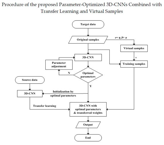
3. Improved Classification Method Based on a Parameter-Optimized Three-Dimensional Convolutional Neural Network (3D-CNN) Combined with Transfer Learning and Virtual Samples

Because the performance of a 3D-CNN could be influenced by its parameter settings, a parameter optimization is proposed in this paper. To solve the problem of limited training samples and to further improve the classification accuracy, an improved method based on a parameter-optimized 3D-CNN combined with transfer learning and virtual samples is also proposed in our HSI classification.

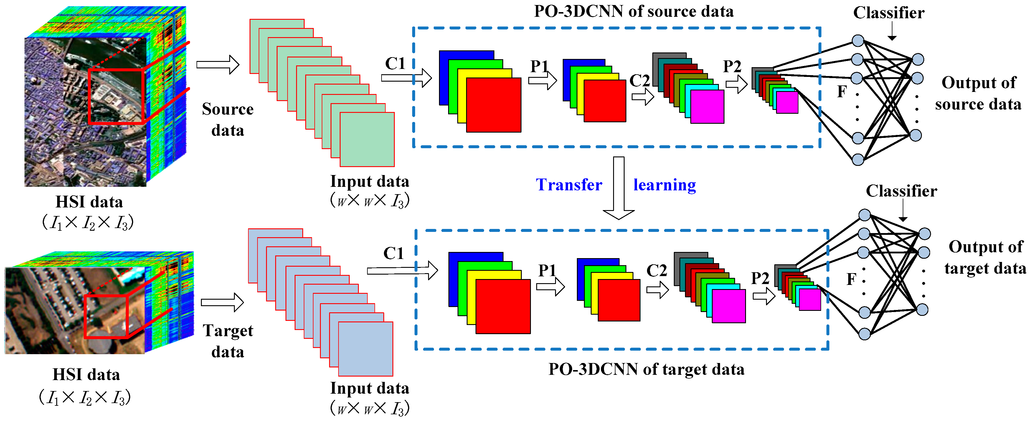
3.1. Parameter-Optimized 3D-CNN (PO-3DCNN)

If the parameter setting of the 3D-CNN is not appropriate, a local minimum loss could be reached and the performance of the network would be greatly degraded [50]. Furthermore, the deeper the network, the more parameters there are. Generally, the setting of network parameters is usually to select the default values or empirical values [51]. In this paper, to optimize the network performance, the parameters of the 3D-CNN are adjusted in turn according to the single variable principle on the basis of experimental results, and the optimal parameters are selected according to the overall accuracy (OA) of classification. Moreover, dropout is introduced in the process of parameter optimization to reduce overfitting.

Firstly, a 3D tensor with a size of w × w × I₃ (w × w and I₃ being the spatial and the spectral sizes respectively) around each sample in the HSI is selected as one of the inputs of the 3D-CNN [52,53].

Secondly, a 3D-CNN with two convolution layers, two pooling layers, and one fully-connected layer can be constructed as an initial network, and softmax regression is used as a classifier.

Thirdly, nine parameters are optimized in this paper: input size, network structure, batch size, number of units in the fully-connected layer, activation function, pooling method, the number of convolutional kernels, the number of epochs, and dropouts. The input size is determined by the size of the input sample; the network structure is mainly affected by the depth of the network and parameters of convolution kernels; during each of the training processes, a part of the training data called batch data is usually used to train the model and update the weights, and the number of samples contained in batch data is called batch size; a process of all the samples in the training data set passing through the network is called one epoch. When one of the nine parameters is being adjusted, the other parameters remain unchanged. The parameters that have been adjusted will be kept at the optimal value. Because most of the references of HSI classification, including the ENVI (Environment for Visualizing Images) software used by remote-sensing professionals and image analysts, have chosen the OA expression as [54], in this paper, in order to facilitate to comparison with the results in other works, the 3D-CNN parameters are optimized in turn according to the single variable principle based on the OA value defined as [54]:

$$OA=\frac{1}{\lambda }{\displaystyle \sum _{r=1}^R{\mathrm{a}}_{rr}}$$

(3)

where λ is the total number of samples, and a_rr is the number of test samples that actually belong to class S_r (r = 1, 2, … R where R is the total number of classes in the HSI) and are also classified into S_r.

Finally, the trained 3D-CNN with the optimal parameters could be used for HSI classification.

However, the limited number of labeled samples in hyperspectral data has a negative impact on the classification results.

3.2. Parameter-Optimized 3D-CNN with Transfer Learning (PO-3DCNN-TL)

Obtaining good network performance under the condition of insufficient samples is important for HSI classification. If there is another HSI (source data) with enough samples and the same feature space as the HSI to be classified (target data), then some weights can be transferred from the network of the source data to that of the target data and fewer training samples will be needed for the network of the target data.

As mentioned in Section 3.1, the initial values of the parameters can also affect the network performance of the 3D-CNN for transfer learning. Therefore, if the 3D-CNN used for transfer learning can be initialized by its optimal parameters, the transferred weights would be more conducive to improving the classification compared with those in a randomly initialized network. This inference has been confirmed by the quantitative experimental results which are not included in the experimental section due to the size and focus of this paper. On the other hand, if the transfer learning was performed before parameter optimization, the classification results were not ideal due to the changes of the transferred weights after parameter optimization having a negative influence on the classification.

Therefore, the flow chart of the parameter-optimized 3D-CNN with transfer learning (PO-3DCNN-TL) is illustrated in Figure 3 where C_k (k = 1, 2) represents the k-th convolution layer, P_k (k = 1, 2) means the k-th pooling layer and F is the abbreviation of the fully-connected layer.

Step 1: a 3D-CNN model of the target data is constructed and its parameters can be optimized according to Section 3.1.

Step 2: another 3D-CNN which has the same framework as that in Step 1 can be constructed and initialized by the optimal parameters obtained in Step 1.

Step 3: the 3D-CNN in Step 2 could be pre-trained by sufficient training samples from the source data. High-level features can be extracted after several convolution and pooling layers.

Step 4: knowledge transfer can be made: the weights in convolutional and pooling layers in the 3D-CNN in Step 1 can be transferred from the same layers of the 3D-CNN in Step 2.

Step 5: to further optimize the network performance, the 3D-CNN in Step 1 will be fine-tuned by the training samples from the target data.

3.3. Virtual Samples

Transfer learning can alleviate the problem of insufficient samples and significantly improve the training efficiency only when the source data are available. If the source data are absent, as a pseudo-sample transformed from the original samples of the image, a virtual sample can also help to solve the problem of insufficient HSI samples. After mixing the virtual samples with the original ones, the overall number of training samples can be greatly increased.

If the original samples in the HSI are presented as a 3D tensor ϑ with a size of w × w × I₃, the virtual sample v can be defined as [32]:

v = ηϑ + n

(4)

where η is the coefficient value close to 1 and can help to reduce the difference between the virtual samples and the original ones, and n denotes the Gaussian noise with zero mean and is used to simulate the interference of the external environment to the samples.

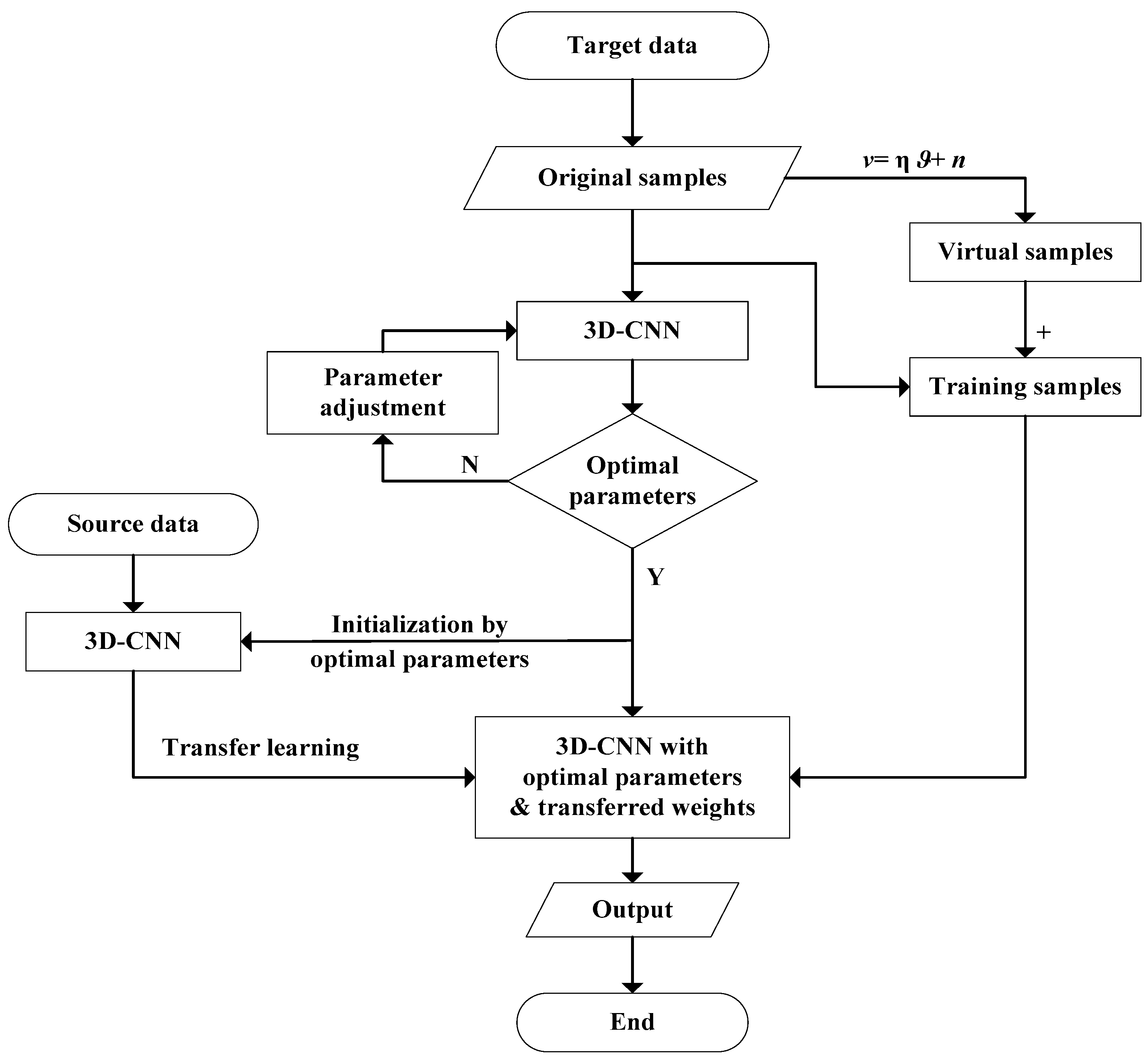
3.4. Parameter-Optimized 3D-CNN Combined with Transfer Learning and Virtual Samples (PO-3DCNN-TV)

Since both transfer learning and virtual samples can make contributions to solve the problem of limited HSI training samples, a hybrid method named PO-3DCNN-TV which combines 3D-CNN, parameter optimization, transfer learning, and virtual samples, is proposed in this paper in order to further improve HSI classification. Figure 4 shows the procedure of the proposed PO-3DCNN-TV method. In Figure 4, a stadium box indicates the beginning and ending of a process, a parallelogram box denotes the process of inputting and outputting data, a rectangular box represents a processing step or a set of operations, and a diamond box shows a conditional operation determining which one of the two paths the program will take.

First of all, based on the original samples of the target data and the OA values of classification, the parameters of the 3D-CNN constructed for the target data can be adjusted to obtain the optimal values as explained in Section 3.1.

Meanwhile, some virtual samples are generated from the original samples and then these two together form the training samples as described in Section 3.3.

Then, another 3D-CNN with the same structure as the network of the target data can be constructed and initialized by the optimal parameters obtained above. It can be trained by the source data to improve the network performance. When the network performance is stable, the weights in the convolution and the pooling layers can be transferred to the corresponding layers in the parameter-optimized 3D-CNN of the target data as mentioned in Section 3.2.

At last, the training samples consisting of the original and the virtual ones can help to pre-train and fine-tune the 3D-CNN model of the target data after parameter optimization and transfer learning, then the results of the improved classification can be obtained.

4. Experiments

In order to evaluate the performance of the proposed classification method, some typical classification methods, such as support vector machines (SVM) [55,56], deep belief networks (DBNs) [57] and 2D-CNNs are compared in the classification experiment of a real-world HSI. To obtain better classification results of 2D-CNNs, the parameter optimization is also introduced to this model in this paper.

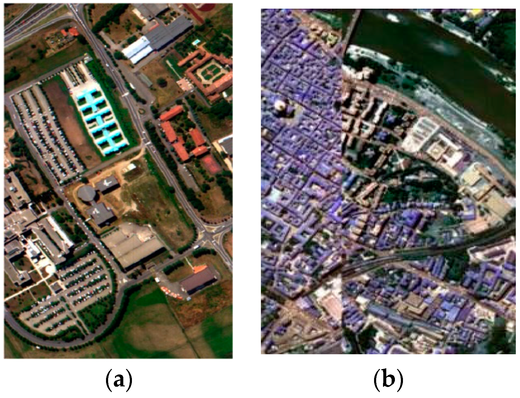
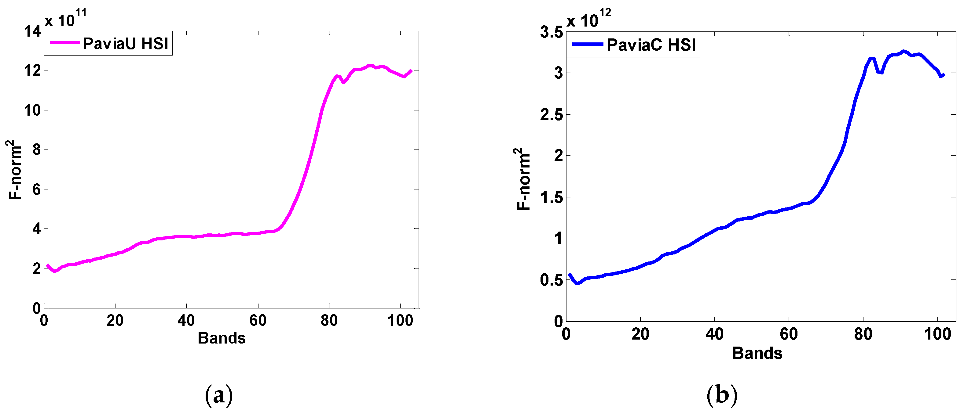
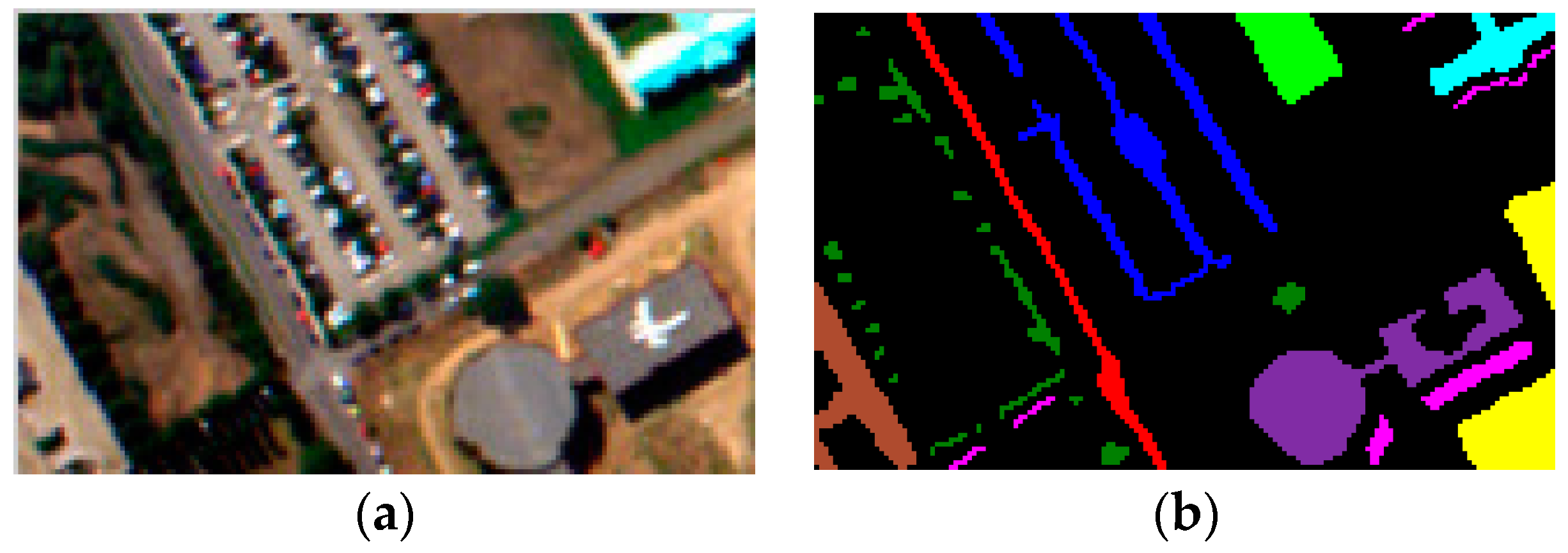
4.1. Real-World Hyperspectral Image (HSI) Data Sets

Two widely used hyperspectral data sets, i.e., the University of Pavia (PaviaU) shown in Figure 5a and the center of Pavia (PaviaC) city shown in Figure 5b are used in the experiment.

Both HSIs are acquired by the Reflective Optics System Imaging Spectrometer (ROSIS) sensor during a flight campaign over the city of Pavia, northern Italy, which makes the disparity between the PaviaU HSI (target data) and the PaviaC HSI (source data) become small. For the Pavia data set, there are strong bands and weak bands; some bands have a higher signal-to-noise level, some bands have a lower signal-to-noise level. In addition, some bands are degraded by random noise, some bands may suffer from residual fixed pattern phenomena, and atmospheric effects may have a different visibility and impact in many bands. Some low-quality bands could be visibly distinguished and should simply be disregarded. Some other noisy bands can be found by denoising algorithms [58]. Therefore, the remaining number of spectral bands is 103 for the PaviaU HSI and 102 for the PaviaC HSI.

In order to further evaluate the data quality of the two HSIs in different bands, a Frobenius norm (F-norm) [59] is introduced:

$${\Vert I(:,:,i_3)\Vert }_F={\left({\displaystyle \sum _{i_1=1}^{I_1}{\displaystyle \sum _{i_2=1}^{I_2}{\left|I(i_1,i_2,i_3)\right|}^2}}\right)}^{\frac{1}{2}}$$

(5)

where I is a tensor consisting of I₁ rows, I₂ columns and I₃ spectral bands with i₁ = 1, …, I₁, i₂ = 1, …, I₂ and i₃ = 1, …, I₃. The smaller the corresponding F-norm value of the image, the lower the corresponding energy, and in consequence, the less useful the information contained. According to Equation (5), the square of the F-norm of each band in two HSIs is shown in Figure 6.

According to Figure 6, the square of F-norm of two HSIs in each band is acceptable; therefore, the above 103 bands of the PaviaU HSI and 102 bands of the PaviaC HSI could all be kept in the experiment. Furthermore, in order to maintain the same number of bands in the two HSIs for transfer learning, the 103-rd spectral dimension of the PaviaC HSI is represented by its original data from the 102-nd dimension.

Taking into account the computational efficiency and the 9 classes contained in the distributed image, one part of the PaviaU (part-PaviaU) HSI is selected as the target data in the experiment. All 9 classes are in the part-PaviaU HSI with a size of 100 × 160 × 103 pixels as shown in Figure 7a,b is its ground truth.

In this paper, 10% of the samples of each class from the part-PaviaU HSI are randomly chosen to train the network and the remaining 90% are for testing. The total number of samples, training samples and testing samples for each class are shown in

Table 1. Land-cover classes and numbers of samples in the part-PaviaU HSI.

No	Color	Class	Total	Testing	Training
1		Asphalt	271	27	244
2		Meadows	277	28	249
3		Gravel	333	33	300
4		Trees	277	28	249
5		Metal sheets	206	21	185
6		Bare Soil	484	48	436
7		Bitumen	758	76	682
8		Bricks	594	59	535
9		Shadow	196	20	176
All classes			3396	340	3056

.

4.2. Parameter Setting of the Considered Classification Methods

4.2.1. Support Vector Machines (SVM)

SVM are one of the supervised learning models [60] and have been applied in classification, regression and outlier detection etc. The effectiveness of a SVM depends mainly on the kernel function which can be well designed by the generalized power spectral density (GPSD) in [56]. In this paper, the SVM in ENVI software [61] is used for the comparison. There are four options for the kernel type of SVM in ENVI: linear, polynomial, radial basis function (RBF) and sigmoid. For SVM classification depending on training and testing samples, the generalization performance of kernels will change with different remote sensing data sets, for instance hyperspectral, and synthetic-aperture radar (SAR), etc. Thus, it is difficult to conclude that any type of kernel can always outperform all other kernel types [62].

In our experiment, taking into account that the polynomial kernel is time-consuming and the linear and sigmoid proved not to perform as well as RBF in HSI classification [62], the RBF is selected as the kernel function of SVM in the ENVI toolbox.

In addition, the hyper-parameters of the RBF kernel, gamma (γ) and penalty factor whose values would affect the classification accuracy, are selected as 100 and 0.01, respectively, for the part-PaviaU HSI through multiple experiments.

4.2.2. Deep Belief Networks (DBN)

A DBN can be stacked by a restricted Boltzmann machine (RBM) to extract features efficiently [63,64]. Because the input of a DBN should be a vector and the HSI is a 3D tensor, in this paper, principal component analysis (PCA) is introduced to reduce the dimension of the HSI, and helps to obtain the one-dimensional (1D) input for the DBN. The 27 × 27 pixel blocks on the first principal component (PC) of the part-PaviaU HSI can be taken and converted into a 1D vector (1 × 729). Then, the input consisting of the 1D vector given above and the 1D spectral vector (1 × 103) of the center pixel in the 27 × 27 pixel blocks can be obtained for the DBN. At last, a DBN of 832-1000-2000-4000-9 units could be constructed. There are 100 epochs of pre-training and 300 epochs of the back-propagation (BP) algorithm.

4.2.3. Parameter-Optimized 2D-CNN (PO-2DCNN)

Since the input data of 2D-CNN should be a matrix, the 1st principal component (PC) of the part-PaviaU HSI is used. By adjusting the parameters mainly according to the OA values, the optimal values of parameters in our 2D-CNN can be obtained as illustrated in

Table 2. Optimal parameters in the PO-2DCNN method.

Parameter	C1	P1	C2	P2	F	Epoch	Act-f	Pooling	Batch
Value	64@5 × 5	64@5 × 5	128@4 × 4	128@2 × 2	128	300	ReLU	Max-pooling	128

where 64@5 × 5 means 64 convolutional kernels with a size of 5 × 5 pixels and act-f means activation function. The size of the input training samples is 27 × 27 for the 1st PC. The weights of the 2D-CNN were randomly initialized with zero mean and a standard deviation of 0.5. Based on the Adadelta algorithm [65], the batch size could be set as 32, and the number of epochs as 300. Dropouts were introduced to prevent overfitting and to improve the network performance. The probabilities of dropout in the P₁, P₂ and F layers are set to 0.5, 0.5 and 0.1 respectively.

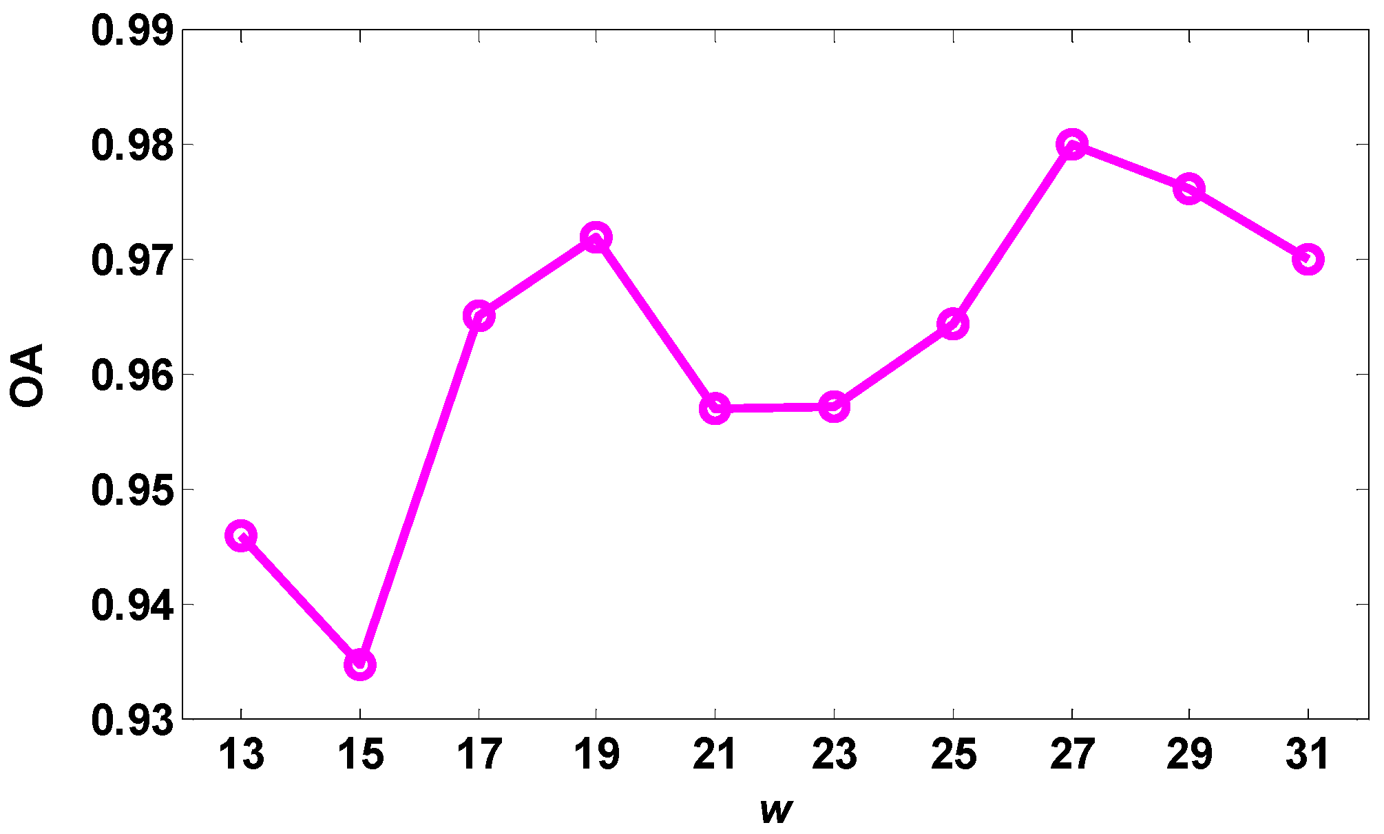
4.3. The Parameters of Some Improved 3D-CNN Models

As a comparison, the improved 3D-CNN models in this paper, for example, the 3D-CNN after parameter optimization (PO-3DCNN), the parameter-optimized 3D-CNN with transfer learning (PO-3DCNN-TL), and the parameter-optimized 3D-CNN with virtual samples (PO-3DCNN-VS) were evaluated and analyzed.

4.3.1. The PO-3DCNN Method

Because the size of input data should be determined first for a 3D-CNN, it is adjusted according to the classification accuracy. In our experiment, for the part-PaviaU HSI, the size of input training samples in the 3D-CNN can be defined as w × w × 103. Under the condition that other network parameters remain unchanged, the relationship between the OA value and w can be seen in Figure 8.

It can be seen from Figure 8 that the OA values reach two peaks when the spatial size w is 19 and 27 respectively. Through a large number of simulations and comprehensive testing of both network classification performance and computational efficiency, 27 was chosen as the optimal spatial size w. For the following experiments, the input size of the 3D-CNN was fixed at 27 × 27 × 103. The optimization process of other parameters is similar to that of the input size.

After parameter optimization, the values of some main parameters of the PO-3DCNN method can be seen in

Table 3. Parameters in the PO-3DCNN method.

Network Layer	Convolutional Layer	Act-F	Pooling Layer	Pooling Function	Dropout
1	4 × 4 × 13@16	ReLU	2 × 2 × 2	Max-pooling	0.1
2	5 × 5 × 13@32	ReLU	2 × 2 × 2	Max-pooling	0.1
3	4 × 4 × 13@64	ReLU	-	-	-

where 4 × 4 × 13@16 indicates 16 3D convolutional kernels with a size of 4 × 4 × 13. The number of convolution kernels in the first layer is 16, the batch size for training is 32 and the number of units in the fully-connected layer is 128, and the dropout in the P₁, P₂ and F layer is set to 0.1.

4.3.2. The PO-3DCNN-TL Method

The PaviaC HSI can be used as the source data to pre-train the 3D-CNN model with optimal parameters and to obtain the weights to be transferred. To ensure the stability of the network performance, 70% of samples of each class in the PaviaC HSI are randomly chosen as the training set and the remaining 30% belong to the testing set. Then, the weights of the convolution and the pooling layers in the 3D-CNN model of the target data, the part-PaviaU HSI, could be transferred from the trained 3D-CNN model of the source data, which can help to improve the feature extraction capability of the network and alleviate the problem of insufficient samples in the target data. After transfer learning, the epoch needed to achieve the peak OA value could be less for the 3D-CNN model of the part-PaviaU HSI and was set to 100 in the experiment. Moreover, fewer samples are enough to train the parameter-optimized 3D-CNN model with transfer learning, and the time required to converge to the optimum is also shorter. Therefore, the introduction of transfer learning can improve the training efficiency of the network and ease the problem of insufficient samples.

4.3.3. The PO-3DCNN-VS method

Virtual samples can be introduced to the parameter-optimized 3D-CNN model according to Equation (4) and η can be set to a uniformly distributed random number in [0.9, 1.1]. The number of virtual samples and the interference n will influence the network performance. Therefore, a sensitivity analysis has been conducted in this paper to achieve better network performance. If the number of original training samples selected from among the target data is T, then the number of virtual samples will be P × T where P represents the ratio between the number of virtual samples and the number of original samples, and the noise variance of n in Equation (4) could be set to 0.01 at the beginning. In the experiment, the virtual and the original samples are mixed together to form the training data set. When the value of the ratio P is different, i.e., when the number of virtual samples is different, the OA value changes. The relationship between P and OA of the part-PaviaU HSI classified by the PO-3DCNN-VS method is shown in Figure 9.

It can be seen from Figure 9 that for the part-PaviaU HSI, the OA value of the PO-3DCNN-VS method changes a little when P is varying, but it reaches the highest value when the number of virtual samples is 1 × T, i.e., the number of virtual samples is equal to the number of original samples. Therefore, the number of virtual samples can be set to T for the PO-3DCNN-VS method in the part-PaviaU HSI classification.

When introducing virtual samples, the noise variance of n will also affect the classification performance. Keeping the number of virtual samples fixed at T and changing the value of the noise variance, denoted as σ², the resulting OA values are shown in

Table 4. OA values vs. different noise variances in the virtual samples.

σ2	0.00001	0.0001	0.001	0.01	0.1	1
OA	0.9927	0.9942	0.9947	0.9936	0.9849	0.9912

.

As presented in Table 4, the OA value is relatively high when the noise variance σ² is less than 0.001. There is a peak at 0.001 which means that the virtual samples are more similar to the original samples at this point. It can also be indicated that the network performance can be improved by adding virtual samples to the training data set in a certain range.

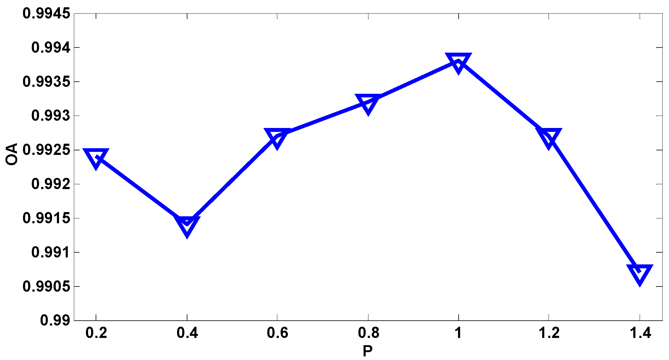
4.4. The Parameters of the Proposed PO-3DCNN-TV Method

As mentioned in Section 4.3.2, a parameter-optimized 3D-CNN model with transfer learning can be constructed for the classification of the part-PaviaU HSI. Meanwhile, the virtual samples with zero mean and noise variance of 0.001 could be generated from the original samples in the part-PaviaU HSI. Then, the virtual samples are mixed with the original ones to pre-train the parameter-optimized 3D-CNN model with transferred weights. Therefore, the values of the corresponding parameters of the proposed PO-3DCNN-TV method for the part-PaviaU HSI are the same as those in Section 4.3.2 and Section 4.3.3.

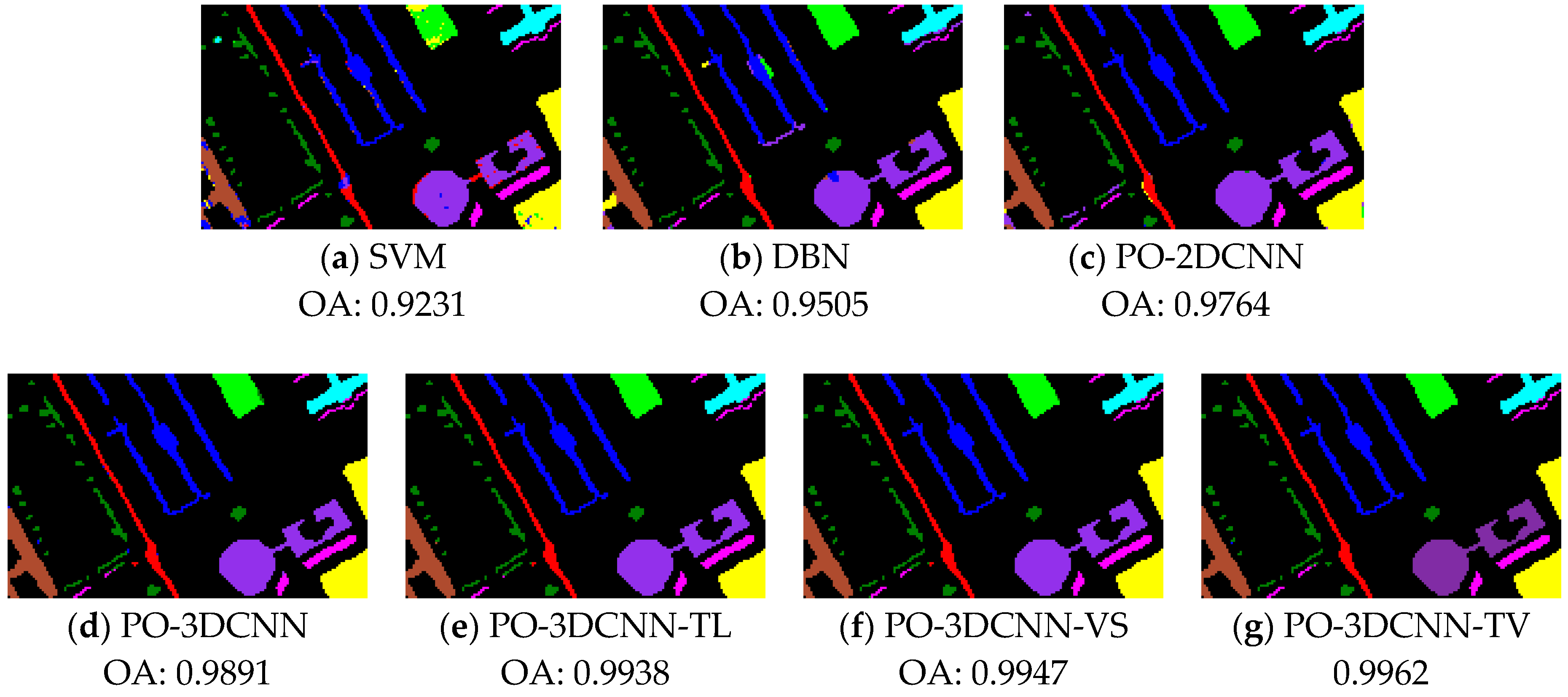
4.5. Classification Results and Discussion

The classification accuracy of the part-PaviaU HSI obtained under different classification models is shown in

Table 5. OA values of nine classes in the part-PaviaU HSI vs. different classification models.

	Classifier	SVM	DBN	PO-2DCNN	PO-3DCNN	PO-3DCNN-TL	PO-3DCNN-VS	PO-3DCNN-TV
Class
Asphalt		0.9004	0.9631	0.9631	0.9815	1	1	1
Meadows		0.7748	0.8949	0.9489	0.9700	1	1	1
Gravel		0.8195	1	1	0.9712	1	0.9928	1
Trees		0.9747	1	0.9134	0.9712	0.9856	0.9892	0.9819
Metal sheets		1	0.9272	0.9757	0.9806	0.9806	0.9757	0.9806
Bare Soil		0.9669	1	0.9773	1	1	1	1
Bitumen		0.9235	0.9670	0.9934	1	1	1	1
Bricks		0.9529	0.8771	1	1	1	1	1
Shadow		1	0.9031	0.9592	0.9439	0.9367	0.9592	0.9796
Overall		0.9231	0.9505	0.9764	0.9891	0.9938	0.9947	0.9962

where the OA values are the average of multiple experiments for each classification model considered in this paper.

It can be seen from Table 5 that SVM has a good performance on metal sheet classification and DBN performs well for gravel, trees and bare soil. A CNN has great potential in the classification of HSIs. With the introduction of transfer learning and virtual samples, the classification accuracy of the 3D-CNN is further improved, especially for the classification of asphalt and meadows.

The classification results obtained by different classification models are shown in Figure 10.

It can be seen from Figure 10 that the classification results of SVM and DBN have more pixels misclassified, especially in the lower part of the image. Our CNN shows superior performance in HSI classification, and a 3D network as shown in Figure 10d performs better than 2D networks as shown in Figure 10c because a 3D-CNN can fully exploit spatial-spectral characteristics in each HSI. Both the introduction of transfer learning as shown in Figure 10e and virtual samples as shown in Figure 10f can alleviate the problem of insufficient samples and reduce the number of misclassified pixels. Virtual samples are helpful for improving the classification performance for the part-PaviaU HSI and the introduction of transfer learning can reduce the computational burden. Therefore, the proposed PO-3DCNN-TV method combining the advantages of the PO-3DCNN-TL and PO-3DCNN-VS helps to greatly improve the classification.

5. Conclusions

To solve the problem of insufficient samples and improve the classification of HSIs, an improved 3D-CNN classification method based on parameter optimization and combined with transfer learning and virtual samples is proposed in this paper. Firstly, the parameters of the 3D-CNN could be adjusted according to the single variable principle. Secondly, the initial weights in the bottom layers of the parameter-optimized 3D-CNN of the target data can be transferred from another 3D-CNN which has been well trained by the source data. Then, some virtual samples are generated from the original samples in the target data. Finally, the parameter-optimized 3D-CNN with transfer learning can be trained by the training samples mixing the original samples in the target data with the virtual samples. Compared with other classification methods considered, the proposed PO-3DCNN-TV method is suitable for the data structure of a HSI and can help to improve the classification.

In future, the residual network will be investigated to further overcome the overfitting problem of a CNN.

References

1. Santara, A.; Mani, K.; Hatwar, P.; Singh, A.; Garg, A.; Padia, K.; Mitra, P. BASS Net: Band-Adaptive Spectral-Spatial Feature Learning Neural Network for Hyperspectral Image Classification. IEEE Trans. Geosci. Remote Sens. 2017, 55, 5293–5301. [Google Scholar] [CrossRef] [Green Version]
2. Fauvel, M.; Chanussot, J.; Benediktsson, J. A spatial–spectral kernel-based approach for the classification of remote-sensing images. Pattern Recognit. 2012, 45, 381–392. [Google Scholar] [CrossRef]
3. Yuan, Y.; Zheng, X.; Lu, X. Spectral–Spatial Kernel Regularized for Hyperspectral Image Denoising. IEEE Trans. Geosci. Remote Sens. 2015, 53, 3815–3832. [Google Scholar] [CrossRef]
4. Mou, L.; Ghamisi, P.; Zhu, X. Deep Recurrent Neural Networks for Hyperspectral Image Classification. IEEE Trans. Geosci. Remote Sens. 2017, 55, 3639–3655. [Google Scholar] [CrossRef]
5. Tuia, D.; Persello, C.; Bruzzone, L. Domain Adaptation for the Classification of Remote Sensing Data: An Overview of Recent Advances. IEEE Geosci. Remote Sens. Mag. 2016, 4, 41–57. [Google Scholar] [CrossRef]
6. Lacar, F.; Lewis, M.; Grierson, I. Use of hyperspectral imagery for mapping grape varieties in the Barossa Valley, South Australia. IGARSS 2001, 6, 2875–2877. [Google Scholar]
7. Gevaert, C.; Suomalainen, J.; Tang, J.; Kooistra, L. Generation of Spectral–Temporal Response Surfaces by Combining Multispectral Satellite and Hyperspectral UAV Imagery for Precision Agriculture Applications. IEEE J. Sel. Top. Appl. Earth Obs. 2015, 8, 3140–3146. [Google Scholar] [CrossRef]
8. Yokoya, N.; Chan, C.; Segl, K. Potential of Resolution-Enhanced Hyperspectral Data for Mineral Mapping Using Simulated EnMAP and Sentinel-2 Images. Remote Sens. 2016, 8, 172. [Google Scholar] [CrossRef]
9. Olmanson, L.G.; Brezonik, P.L.; Bauer, M. Airborne hyperspectral remote sensing to assess spatial distribution of water quality characteristics in large rivers: The Mississippi River and its tributaries in Minnesota. Remote Sens. Environ. 2013, 130, 254–265. [Google Scholar] [CrossRef]
10. Wu, C.; Du, B.; Zhang, L. Slow Feature Analysis for Change Detection in Multispectral Imagery. IEEE Trans. Geosci. Remote Sens. 2014, 52, 2858–2874. [Google Scholar] [CrossRef]
11. Laurin, G.V.; Chan, C.W.; Chen, Q.; Lindsell, J.A.; Coomes, D.A.; Guerriero, L.; Frate, F.D.; Miglietta, F.; Valentini, R. Biodiversity Mapping in a Tropical West African Forest with Airborne Hyperspectral Data. PLoS ONE 2014, 9, e97910. [Google Scholar]
12. Demir, B.; Bovolo, F.; Bruzzone, L. Updating Land-Cover Maps by Classification of Image Time Series: A Novel Change-Detection-Driven Transfer Learning Approach. IEEE Trans. Geosci. Remote Sens. 2013, 51, 300–312. [Google Scholar] [CrossRef]
13. Dev, S.; Wen, B.; Lee, Y.H.; Winkler, S. Ground-Based Image Analysis: a Tutorial on Machine-Learning Techniques and Applications. IEEE Geosci. Remote Sens. Mag. 2016, 4, 79–93. [Google Scholar] [CrossRef]
14. Bioucas-Dias, J.M.; Plaza, A.; Camps-Valls, G.; Scheunders, P.; Nasrabadi, N.; Chanussot, J. Hyperspectral Remote Sensing Data Analysis and Future Challenges. IEEE Geosci. Remote Sens. Mag. 2013, 1, 6–36. [Google Scholar] [CrossRef] [Green Version]
15. Hang, R.; Liu, Q.; Song, H.; Sun, Y. Matrix-Based Discriminant Subspace Ensemble for Hyperspectral Image Spatial-Spectral Feature Fusion. IEEE Trans Geosci. Remote Sens. 2016, 54, 783–794. [Google Scholar] [CrossRef]
16. Hang, R.; Liu, Q.; Sun, Y.; Yuan, X.; Pei, H. Robust matrix discriminative analysis for feature extraction from hyperspectral images. IEEE J. Sel. Top. Appl. Earth Obs. 2017, 10, 2002–2011. [Google Scholar] [CrossRef]
17. Xu, Y.; Zhang, L.; Du, B.; Zhang, F. Spectral-Spatial Unified Networks for Hyperspectral Image Classification. IEEE Trans. Geosci. Remote Sens. 2018, 1–17. [Google Scholar] [CrossRef]
18. Song, H.; Liu, Q.; Wang, G.; Hang, R.; Huang, B. Spatiotemporal Satellite Image Fusion Using Deep Convolutional Neural Networks. IEEE J. Sel. Top. Appl. Earth Obs. 2018, 11, 821–829. [Google Scholar] [CrossRef]
19. Liu, W.; Yang, X.; Tao, D.; Cheng, J.; Tang, Y. Multiview dimension reduction via Hessian multiset canonical correlations. Inf. Fusion 2018, 41, 119–128. [Google Scholar] [CrossRef]
20. Wang, M.; Hua, X.; Hong, R.; Tang, J.; Qi, G.; Song, Y. Unified video annotation via multigraph learning. IEEE Trans. Circuits Syst. Video Technol. 2009, 19, 733–746. [Google Scholar] [CrossRef]
21. Yang, X.; Liu, W.; Tao, D.; Cheng, J.; Li, S. Multiview Canonical Correlation Analysis Networks for Remote Sensing Image Recognition. IEEE Geosci. Remote Sens. Lett. 2017, 14, 1855–1859. [Google Scholar] [CrossRef]
22. Wang, M.; Hua, X.S. Active learning in multimedia annotation and retrieval: A survey. Acm Trans. Intell. Syst. Technol. 2011, 2, 1–21. [Google Scholar] [CrossRef]
23. Hu, J.; He, Z.; Li, J.; He, L.; Wang, Y. 3D-Gabor Inspired Multiview Active Learning for Spectral-Spatial Hyperspectral Image Classification. Remote Sens. 2018, 10, 1070. [Google Scholar] [CrossRef]
24. Lee, G. Fast computation of the compressive hyperspectral imaging by using alternating least squares methods. Signal Process. Image Comm. 2018, 60, 100–106. [Google Scholar] [CrossRef]
25. Wang, L.; Bai, J.; Wu, J.; Jeon, G. Hyperspectral image compression based on lapped transform and Tucker decomposition. Signal Process. Image Commun. 2015, 36, 63–69. [Google Scholar] [CrossRef]
26. Yang, W.; Yin, X.; Xia, G.S. Learning High-level Features for Satellite Image Classification with Limited Labeled Samples. IEEE Trans. Geosci. Remote Sens. 2015, 53, 4472–4482. [Google Scholar] [CrossRef]
27. Cvetković, S.; Stojanovic, M.; Nikolić, S. Multi-channel descriptors and ensemble of Extreme Learning Machines for classification of remote sensing images. Signal Process. Image Commun. 2015, 39, 111–120. [Google Scholar] [CrossRef]
28. Zhao, F.; Liu, G.; Wang, X. An efficient macroblock-based diverse and flexible prediction modes selection for hyperspectral images coding. Signal Process. Image Commun. 2010, 25, 697–708. [Google Scholar] [CrossRef]
29. Vakil, M.; Megherbi, D.; Malas, J. A robust multi-stage information-theoretic approach for registration of partially overlapped hyperspectral aerial imagery and evaluation in the presence of system noise. Image Commun. 2017, 52, 97–110. [Google Scholar] [CrossRef]
30. Huang, Z.; Pan, Z.; Lei, B. Transfer Learning with Deep Convolutional Neural Network for SAR Target Classification with Limited Labeled Data. Remote Sens. 2017, 9, 907. [Google Scholar] [CrossRef]
31. Chen, Y.; Lin, Z.; Zhao, X.; Wang, G.; Gu, Y. Deep Learning-Based Classification of Hyperspectral Data. IEEE J. Sel. Top. Appl. Earth Obs. 2014, 7, 2094–2107. [Google Scholar] [CrossRef]
32. Chen, Y.; Jiang, H.; Li, C.; Jia, X.; Ghamisi, P. Deep Feature Extraction and Classification of Hyperspectral Images Based on Convolutional Neural Networks. IEEE Trans. Geosci. Remote Sens. 2016, 54, 6232–6251. [Google Scholar] [CrossRef]
33. Mei, S.; Yuan, X.; Ji, J.; Zhang, Y.; Wan, S. Hyperspectral Image Spatial Super-Resolution via 3D Full Convolutional Neural Network. Remote Sens. 2017, 9, 1139. [Google Scholar] [CrossRef]
34. Cao, J.; Chen, Z.; Wang, B. Graph-based deep Convolutional networks for Hyperspectral image classification. IGARSS 2016, 3270–3273. [Google Scholar]
35. Liu, W.; Zha, Z.; Wang, Y.; Lu, K.; Tao, D. p-Laplacian Regularized Sparse Coding for Human Activity Recognition. IEEE Trans. Ind. Electron. 2016, 63, 5120–5129. [Google Scholar] [CrossRef]
36. Liu, W.; Liu, H.; Tao, D.; Wang, Y.; Lu, K. Manifold regularized kernel logistic regression for web image annotation. Neurocomputing 2016, 172, 3–8. [Google Scholar] [CrossRef]
37. Yu, M.; Dong, G.; Fan, H.; Kuang, G. SAR target recognition via local sparse representation of Multi-Manifold regularized Low-Rank approximation. Remote Sens. 2018, 10, 211. [Google Scholar]
38. Casale, P.; Altini, M.; Amft, O. Transfer Learning in Body Sensor Networks Using Ensembles of Randomised Trees. IEEE Int. Things J. 2015, 2, 33–40. [Google Scholar] [CrossRef]
39. Yang, J.; Zhao, Y.; Chan, C. Learning and Transferring Deep Joint Spectral–Spatial Features for Hyperspectral Classification. IEEE Trans. Geosci. Remote Sens. 2017, 55, 4729–4742. [Google Scholar] [CrossRef]
40. Pan, S.; Yang, Q. A Survey on Transfer Learning. IEEE Trans. Knowl. Data Eng. 2010, 22, 1345–1359. [Google Scholar] [CrossRef] [Green Version]
41. Oquab, M.; Bottou, L.; Laptev, I.; Sivic, J. Learning and Transferring Mid-level Image Representations Using Convolutional Neural Networks. CVPR 2014, 1717–1724. [Google Scholar] [Green Version]
42. Lin, J.; He, C.; Wang, Z.; Li, S. Structure Preserving Transfer Learning for Unsupervised Hyperspectral Image Classification. IEEE Geosci. Remote Sens. Lett. 2017, 14, 1656–1660. [Google Scholar] [CrossRef]
43. Fielding, J.; Fox, L.; Heller, H.; Seltzer, S.; Tempany, C. Spiral CT in the evaluation of flank pain: Overall accuracy and feature analysis. J. Comput. Assist. Tomogr. 1997, 21, 635–638. [Google Scholar] [CrossRef] [PubMed]
44. Radford, A.; Metz, L.; Chintala, S. Unsupervised Representation Learning with Deep Convolutional Generative Adversarial Network. arXiv, 2015; arXiv:1511.06434. [Google Scholar]
45. Zhong, Z.; Li, J.; Luo, Z.; Chapman, M. Spectral-spatial residual network for hyperspectral image classification: A 3-D deep learning framework. IEEE Trans. Geosci. Remote Sens. 2018, 56, 847–858. [Google Scholar] [CrossRef]
46. Li, Y.; Zhang, H.; Shen, Q. Spectral-Spatial Classification of Hyperspectral Imagery with 3D Convolutional Neural Network. Remote Sens. 2017, 9, 67. [Google Scholar] [CrossRef]
47. Hinton, G.; Srivastava, N.; Krizhevsky, A.; Sutskever, I.; Salakhutdinov, R. Improving neural networks by preventing co-adaptation of feature detectors. Comput. Sci. 2012, 3, 212–223. [Google Scholar]
48. Glorot, X.; Bordes, A.; Bengio, Y. Deep Sparse Rectifier Neural Networks. AISTATS 2011, 315–323. [Google Scholar]
49. Zuo, Z.; Shuai, B.; Wang, G.; Liu, X.; Wang, X.; Wang, B.; Chen, Y. Learning Contextual Dependence with Convolutional Hierarchical Recurrent Neural Networks. IEEE Trans. Image Process. 2016, 25, 2983–2996. [Google Scholar] [CrossRef] [PubMed]
50. Ghamisi, P.; Chen, Y.; Zhu, X. A Self-Improving Convolution Neural Network for the Classification of Hyperspectral Data. IEEE Geosci. Remote Sens. Lett. 2016, 13, 1537–1541. [Google Scholar] [CrossRef]
51. Bengio, Y. Practical Recommendations for Gradient-Based Training of Deep Architectures. Lect. Notes Comput. Sci. 2012, 7700, 437–478. [Google Scholar] [Green Version]
52. Jia, S.; Hu, J.; Zhu, J.; Jia, X.; Li, Q. Three-Dimensional Local Binary Patterns for Hyperspectral Imagery Classification. IGARSS 2016, 55, 465–468. [Google Scholar]
53. Wu, Z.; Wang, Q.; Shen, Y. 3D gray-gradient-gradient tensor field feature for hyperspectral image classification. In Proceedings of the 10th International Conference on Communications and Networking in China (ChinaCom), Shanghai, China, 15–17 August 2015; pp. 432–436. [Google Scholar]
54. Liu, X.; Bourennane, S.; Fossati, C. Denoising of Hyperspectral Images Using the PARAFAC Model and Statistical Performance Analysis. IEEE Trans. Geosci. Remote Sens. 2012, 50, 3717–3724. [Google Scholar] [CrossRef]
55. Anguita, D.; Ridella, S.; Rivieccio, F. K-fold generalization capability assessment for support vector classifiers. IJCNN 2005, 2, 855–858. [Google Scholar]
56. Zorzi, M.; Chiuso, A. The Harmonic Analysis of Kernel Functions. Automatica 2018, 94, 125–137. [Google Scholar] [CrossRef]
57. Chen, Y.; Zhao, X.; Jia, X. Spectral–Spatial Classification of Hyperspectral Data Based on Deep Belief Network. IEEE J. Sel. Top. Appl. Earth Obs. 2015, 8, 2381–2392. [Google Scholar] [CrossRef]
58. Liu, X.; Bourennane, S.; Fossati, C. Reduction of Signal-Dependent Noise from Hyperspectral Images for Target Detection. IEEE Trans. Geosci. Remote Sens. 2014, 52, 5396–5411. [Google Scholar]
59. Zhao, W.; Zhang, H. Secure Fingerprint Recognition Based on Frobenius Norm. In Proceedings of the International Conference on Computer Science and Electronics Engineering, Hangzhou, China, 23–25 March 2012; pp. 388–391. [Google Scholar]
60. Wieland, M.; Liu, W.; Yamazaki, F. Learning Change from Synthetic Aperture Radar Images: Performance Evaluation of a Support Vector Machine to Detect Earthquake and Tsunami-Induced Changes. Remote Sens. 2016, 8, 792. [Google Scholar] [CrossRef]
61. ENVI (Version 5.5)-Online Help, Using ENVI, Support Vector Machine. Available online: https://www.harrisgeospatial.com/docs/SupportVectorMachine.html (accessed on 23 August 2018).
62. Ustuner, M.; Sanli, F.B.; Dixon, B. Application of Suport Vector Machines for Landuse Classification Using High-Resolution RapidEye Images: A Sensitivity Analysis. J. Remote Sens. 2015, 48, 403–422. [Google Scholar]
63. Li, J.; Xi, B.; Li, Y.; Du, Q.; Wang, K. Hyperspectral Classification Based on Texture Feature Enhancement and Deep Belief Networks. Remote Sens. 2018, 10, 396. [Google Scholar] [CrossRef]
64. Bu, Y.; Zhao, G.; Luo, A.; Pan, J.; Chen, Y. Restricted Boltzmann machine: A non-linear substitute for PCA in spectral processing. Astron. Astrophys. 2015, 576, A96. [Google Scholar] [CrossRef]
65. Zeiler, M.D. ADADELTA: An Adaptive Learning Rate Method. arXiv, 2012; arXiv:1212.5701. [Google Scholar]
Figure 1. Framework of a three-dimensional convolutional neural network (3D-CNN).
Remotesensing 10 01425 g001
Figure 2. Illustration of the 3D convolution.
Remotesensing 10 01425 g002
Figure 3. Flow chart of the parameter-optimized 3D-CNN with transfer learning.
Remotesensing 10 01425 g003
Figure 4. Procedure of the proposed parameter-optimized 3D-CNN combined with transfer learning and virtual samples (PO-3DCNN-TV) method.
Remotesensing 10 01425 g004
Figure 5. Hyperspectral images (HSIs) of Pavia city. (a) PaviaU HSI. (b) PaviaC HSI.
Remotesensing 10 01425 g005
Figure 6. Square of the Frobenius norm (F-norm) of Pavia city HSIs. (a) PaviaU HSI. (b) PaviaC HSI.
Remotesensing 10 01425 g006
Figure 7. (a) Part-PaviaU HSI. (b) Ground truth.
Remotesensing 10 01425 g007
Figure 8. The overall accuracy (OA) values vs different spatial size w of the input data.
Remotesensing 10 01425 g008
Figure 9. OA values vs different ratio P between the number of virtual and original samples.
Remotesensing 10 01425 g009
Figure 10. Classification of the part-PaviaU HSI.
Remotesensing 10 01425 g010