Integrating Aerial and Street View Images for Urban Land Use Classification
by
 , , ,
, , ,
Rui Cao
1,2,3 ,
,
Jiasong Zhu
1,
Wei Tu
1,
Qingquan Li
1,4,
Jinzhou Cao
4,
Bozhi Liu
2,
Qian Zhang
3 and
Guoping Qiu
2,5,* 1
Shenzhen Key Laboratory of Spatial Smart Sensing and Services & Key Laboratory for Geo-Environmental Monitoring of Coastal Zone of the National Administration of Surveying, Mapping and GeoInformation, Shenzhen University, Shenzhen 518060, China
2
College of Information Engineering & Guangdong Key Laboratory of Intelligent Information Processing, Shenzhen University, Shenzhen 518060, China
3
International Doctoral Innovation Centre & School of Computer Science, University of Nottingham Ningbo China, Ningbo 315100, China
4
State Key Laboratory of Information Engineering in Surveying, Mapping, and Remote Sensing, Wuhan University, Wuhan 430079, China
5
School of Computer Science, University of Nottingham, Nottingham NG8 1BB, UK
*
Author to whom correspondence should be addressed.
Remote Sens. 2018, 10(10), 1553; https://0-doi-org.brum.beds.ac.uk/10.3390/rs10101553
Submission received: 29 August 2018
/
Revised: 20 September 2018
/
Accepted: 25 September 2018
/
Published: 27 September 2018
(This article belongs to the Special Issue Image Retrieval in Remote Sensing)
Abstract
:Urban land use is key to rational urban planning and management. Traditional land use classification methods rely heavily on domain experts, which is both expensive and inefficient. In this paper, deep neural network-based approaches are presented to label urban land use at pixel level using high-resolution aerial images and ground-level street view images. We use a deep neural network to extract semantic features from sparsely distributed street view images and interpolate them in the spatial domain to match the spatial resolution of the aerial images, which are then fused together through a deep neural network for classifying land use categories. Our methods are tested on a large publicly available aerial and street view images dataset of New York City, and the results show that using aerial images alone can achieve relatively high classification accuracy, the ground-level street view images contain useful information for urban land use classification, and fusing street image features with aerial images can improve classification accuracy. Moreover, we present experimental studies to show that street view images add more values when the resolutions of the aerial images are lower, and we also present case studies to illustrate how street view images provide useful auxiliary information to aerial images to boost performances.
1. Introduction
Urban areas account for less than 2% of the earth land surface, but accommodate more than half of the world population, and the urban population is still growing and is estimated to reach five billion by 2030 globally [1]. The unprecedented urbanization leads to rapid changes of urban surface, it is therefore of great significance to monitor our urban land so as to provide essential information to decision makers to better manage our cities and provide supports for sustainable development.
Urban land use and land cover (LULC) maps are very important tools to understand and monitor our cities, they can reflect the macro properties of the urban surface. Specifically, land cover indicates the physical attributes of landscapes, such as forestry, grass, agricultural, water bodies, built-up areas, etc., while land use documents how people use the land with social-economic purposes, such as residential, commercial, and recreational purposes. The classification of urban land use is very difficult, especially for mega-cities with high population density where land use is extremely diversified and complicated.
Earth observation data such as multi-spectral satellite images have long been used to classify different land covers in terms of spectral reflectance characteristics of different objects [2]. However, most of them are of medium spatial resolution, and are not well suited for categorizing urban land use types of different social-economic properties [2,3]. Urban land use classification still relies heavily on labor-intensive land survey [1], which are inefficient and expensive.
With the development of geospatial technologies, we are able to acquire very high resolution (VHR) satellite and aerial images, which enables us to acquire more texture details from overhead images than before. Traditional spectral-based classification methods may fail for VHR imagery, because the improvement of geometrical resolution increases intra-class variance and causes more inter-class spectral confusion [2]. As a consequence, more texture features need to be extracted from VHR imagery for land use classification. The situation is eased with the great progress of deep neural networks (DNNs) made in computer vision applications [4], and the breakthroughs on semantic segmentation tasks [5] especially facilitates the pixel-level urban land use classification problem [6].
Despite great increase in spatial resolution, urban land use classification from overhead images is still regarded as a difficult task [7], because only the top of the cities can be captured from nadir view. The lack of ground-level details makes it hard to predict social-economic usage purposes of urban land. Fortunately, the growing accessibility to different sources of geo-tagged data makes it possible to fuse remote sensing imagery with data of different modalities and observations [8]. For example, Google Street View (GSV) [9] serves users with street-level panoramic imagery captured in thousands of cities worldwide, which makes it possible to observe street scenes in big cities and thus provides proximate sensing ability and ground-level details that overhead images lack.
Zhang et al. [10] have pioneered the integration of airborne LiDAR, high resolution orthoimagery, and Google Street View for parcel-level urban land use classification. The work demonstrates that ground-level street view images are useful for classifying urban land parcels. However, the work relies on given land parcels as prior classification units, which limits the application scenarios where land parcels are not available.
To bridge the gap, in this paper, we use a deep neural network to extract features from geo-tagged street view images and interpolate them in the spatial domain, and we further present a deep learning-based approach to fusing the extracted features with high-resolution aerial images for urban land use classification in pixel level. The methods are tested on a large publicly available dataset and proven to be effective. We have also examined the impact of aerial image resolution changes on classification results. Moreover, we have investigated into the roles that street view images play in refining classification results by case studies. The contributions of the paper lie in three aspects: (1) The paper presents a novel method to fuse extracted ground-level features from street view images with high-resolution aerial images to enhance pixel-level urban land use classification accuracy. It integrates the two sources of images collected from totally different views (i.e., overhead and ground-level views), and therefore demonstrates a new possibility and paradigm of multi-source and multi-modal data fusion for urban land use classification; (2) The paper examines the impact of aerial image resolution changes on classification accuracy, and it also presents case studies to investigate into the contribution that street view images make to the improvement of the classification results; (3) This paper explores deep neural network methods for pixel-level urban land use classification using high-resolution aerial images, which enriches the remote sensing applications of deep neural networks.
The rest of the paper is organized as follows. In Section 2, we review related work on land use and land cover classification and current research progress on semantic segmentation using deep neural networks. Section 3 describes the methods we use to construct ground feature maps from street view images, and integrate overhead and ground-level images for urban land use classification. In Section 4, we test our methods on a publicly available dataset of large aerial and street view images and analyze the results, and we also investigate into the impact of aerial image resolution changes on semantic segmentation results. In Section 5, we discuss the classification results and present case studies on the improvement of accuracy by integrating street view images. Finally, we conclude in Section 6.
2. Related Work
2.1. Land Use and Land Cover Classification
Remote sensing: Land use and land cover classification via satellite images have been extensively studied in remote sensing community. Most related work has engaged with land cover classification [1,3,7], and normally, the inference of specific land cover types more relies on spectral-based classification [2], because the spatial resolution of remote sensing images in visible bands is limited. With the development of geospatial technologies, very high resolution satellite and aerial images become more available, which enables us to analyze more spatial patterns via these images [2,11,12,13]. Albert et al. [14] use satellite imagery to identify urban land use patterns. Hu et al. [15] classify urban land use categories using remote sensing imagery given land parcels. Hernandez et al. [16] categorize land use integrating spatial metrics and texture analysis. Lv et al. [17] use remote sensing SAR imagery for urban land use and land cover classification. Most remote sensing-based LULC classification work focuses on spectral-based land cover classification, however, with the growing accessibility to VHR remote sensing imagery and ground-level geo-tagged proximate sensing data, there are more opportunities to infer urban land use of social-economic properties.
Proximate sensing: Traditional land use map is provided by labor-intensive land survey [1] which is time-consuming and expensive. To alleviate the situation, researchers have tried to infer land use from proximate sensing data. Pei et al. [18] use aggregated mobile phone data to conduct land use classification in mesh grid level. Zhu et al. [7] use ground-level geo-referenced images from Flickr to do land use mapping based on land parcel map. Antoniou et al. [19] have investigated geo-tagged social media images as land cover input data and prove that these data include useful information about land use and land cover. Torres et al. [20] show that ground-taken imagery contains more useful details than overhead imagery for fine-grained habitat classification. Zhang et al. [10] and Kang et al. [21] use street view images to classify building functions given building footprints. Tu et al. [22] and Cao et al. [23] couple mobile phone data and social media check-in data to infer urban land function zones. Yuyun et al. [24] use Twitter data to acquire dynamic land use map. Tu et al. [25] and Liu et al. [26] demonstrate that public transport mobility data also implies urban land use variation. These works demonstrate that ground-level geo-tagged data contain useful information for land use and land cover classification. However, because of the lack of global view, most proximate sensing-based work relies on given land parcels as prior statistic units which limits the application scenarios.
Multimodal data fusion: Remote and proximate sensing data include macro overhead and micro ground-level information, respectively. The integration of them is believed to be able to capture both information and therefore provide more insights into the understanding of urban land use distribution than just use one data source alone. Tu et al. [1] and Jia et al. [3] integrate satellite images and mobile phone positioning data to generate urban land use maps. Liu et al. [27] and Hu et al. [28] combine satellite images and POIs (points of interest) to classify urban land parcels, showing that social media data have the potential for augmenting LULC classification. Jendryke et al. [29] integrate SAR imagery and social media message data to acquire urban land use information. Some researches also try to fuse data of different views in terms of physical appearance of urban surface [8] to estimate geospatial functions [30,31], classify urban land parcels [10], and analyze city land surface conditions [32,33]. Data of different sources and modalities possess different information about targeted objects, however, it is not easy to fuse them directly because of the heterogeneity of data distribution and various demands of specific applications. Thus, it is of great value to develop methods to fuse data of different sources and modalities to improve urban land use classification. The paper therefore presents an effective method to extract features from street view images, and further fuse them to aerial images to categorize urban land use in pixel level.
2.2. DNN-based Semantic Segmentation
With the unprecedented success of deep neural networks, many computer vision applications have seen great breakthroughs, including image classification [34,35,36,37], object detection [38,39,40], and semantic segmentation [5,41,42].
Fully Convolutional Network (FCN) [41] is regarded as a milestone for DNN-based semantic segmentation. Ever since it is proposed to solve the pixel-level classification problem, more and more semantic segmentation researches have focused on deep neural networks methods. The network changes the architecture of normal deep convolutional neural networks for classification by replacing fully connection layers with convolutional layers which enable it to make dense pixel-level predictions, this paradigm is adopted by many DNN-based semantic segmentation methods followed [5,42]. FCN has its drawbacks, and the most significant problem is its pooling layer, which can aggregate information and extract spatial-invariant features. However, spatial information is crucial for semantic segmentation problems since pixel-level predictions are to be made. To address the problem, two main architectures are proposed, the first one is encoder-decoder architecture, such as U-Net [43], SegNet [42], FC-DenseNet [44], and the other is the use of dilated convolutions, such as DeepLab [45,46,47]. Some researches also add post-processing stage by using a Conditional Random Field (CRF) [45,48].
Most breakthroughs in DNN-based semantic segmentation happened on natural images [5]. However, remote sensing images are very different from ordinary natural images. Some efforts and progresses have been made on satellite and aerial image segmentation using deep learning approaches [6]. Convolutional neural networks like patch-based and pixel-to-pixel based network [13], self-cascaded network [49], hourglass-shape network [50], gated network [51], and dual multi-scale manifold ranking-based network [52] have been proposed for land cover mapping using very high resolution aerial images based on the dataset from ISPRS 2D Semantic Labeling Challenge [53]. Moreover, CNNs for multi-modal fusion of aerial images and DSM (digital surface model) data have also been investigated [11,12,54]. Most DNN-based semantic segmentation researches focus on land cover classification of limited categories; however, the possibilities on categorizing land use categories have not been fully explored yet. On the other hand, the integration of ground-level geo-tagged data is also to be examined. Our work enriches the research on urban land use classification on VHR remote sensing images, and further investigates into the method of integrating ground-level data to improve classification results.
3. Methodology
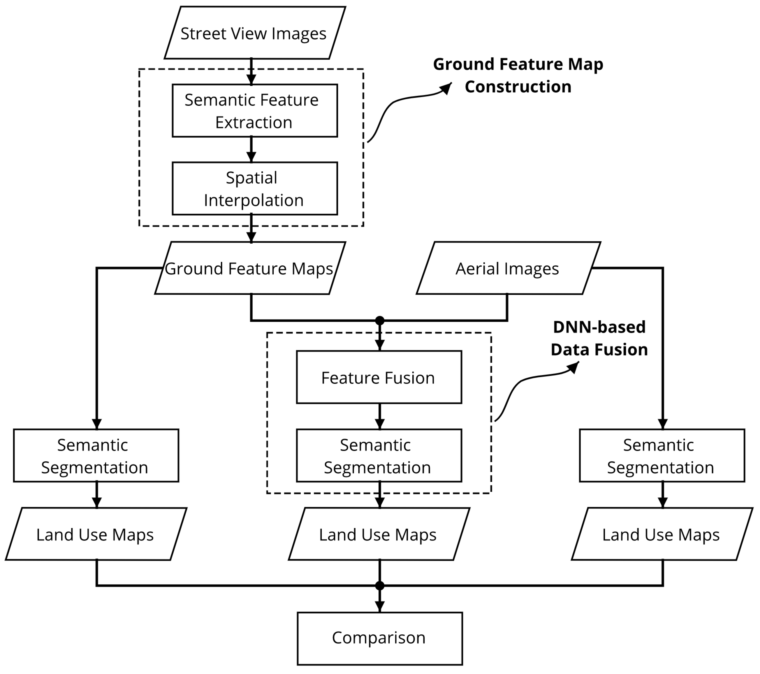
To use ground-level street view images for urban land use classification, we propose an approach to construct ground feature maps from street view images and further integrate them with remote sensing aerial images, the workflow is illustrated in Figure 1. Specifically, semantic features are firstly extracted from street view images, and then ground feature maps are constructed by interpolating those features in the spatial domain. After that, both aerial images and ground feature maps are taken as inputs to the proposed deep convolutional neural network, which is able to fuse the two sources of data from different views. Finally, the segmentation results of coupling aerial and ground images are compared with that of using one source of images only.
3.1. Ground Feature Map Construction
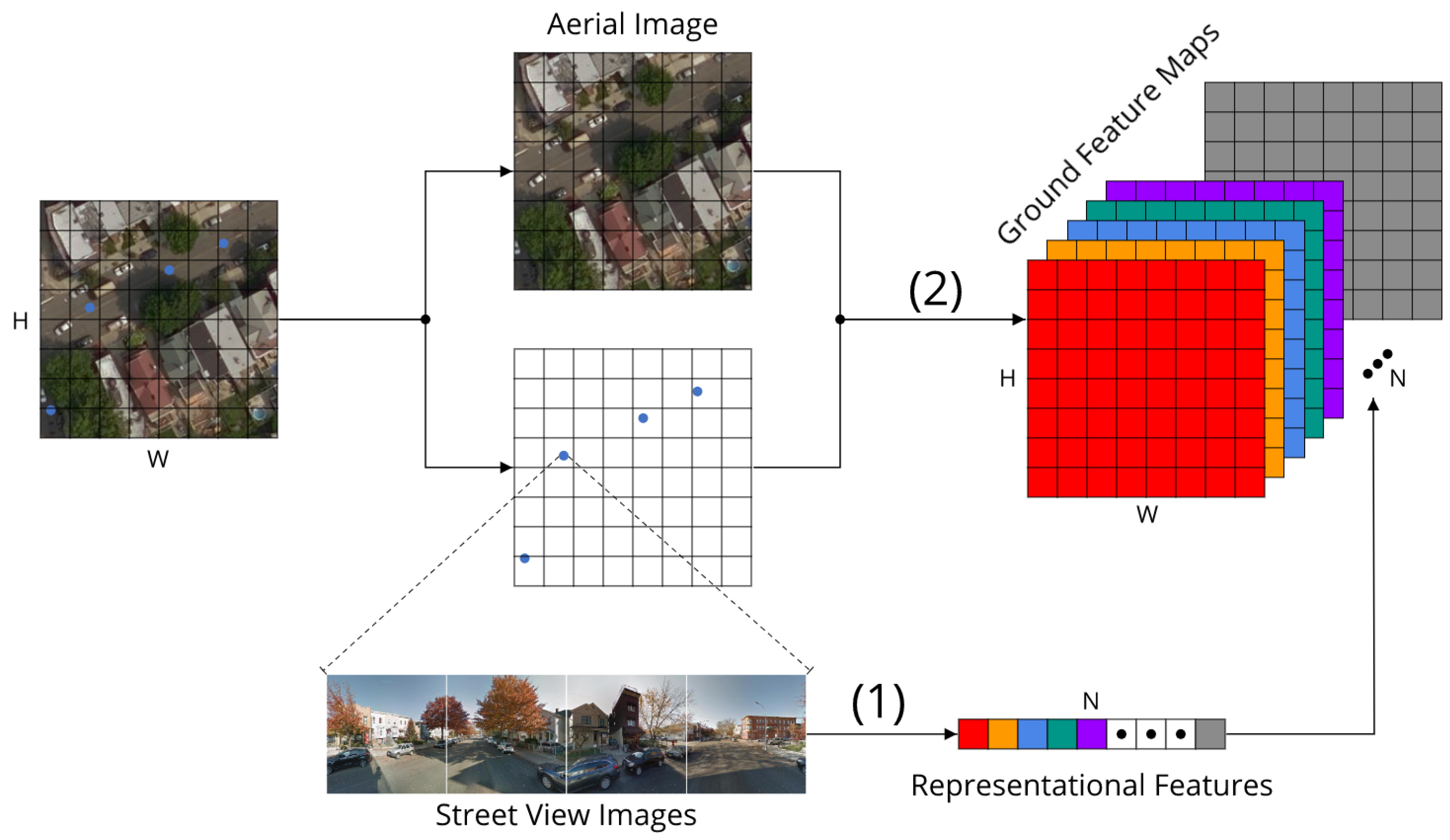
In order to align ground-level street view images with overhead aerial images in pixel level, we present a method to construct ground feature maps from street view images. Basically, there are two major steps, i.e., semantic feature extraction and spatial interpolation. The construction process is illustrated in Figure 2.
3.1.1. Semantic Feature Extraction
Deep neural networks are reported to be effective to extract useful semantic information from street view images [21,30,55]. In our study, semantic features of street view images are firstly extracted by Places-CNN which is a deep convolutional neural network used for ground-level scene recognition. The network is trained on the Places365 dataset [56], a ten-million large image database of real-world scene photographs labeled with diverse scene semantic categories. The extracted semantic features are able to reflect the semantic information of particular scenes which are captured near the collecting spots of street view images, and they are capable of providing ground-level details for urban land use mapping.
As it is shown in Figure 2, locations with street view images are symbolized by blue dots, and there are four street view images facing different directions for each location which capture the panorama scene of the spot. We first use a pretrained Places-CNN (without the last fully connection layer) to extract a 512-dimensional feature vector for each image, and then concatenate the extracted four feature vectors into a 2048-dimensional feature vector for each location. After that, principal component analysis (PCA) is used to compress semantic information and reduce the dimension of the feature vector to 50, which finally produce the representational semantic features for the locations.
3.1.2. Spatial Interpolation
As it can be seen from Figure 2, places with street view images are sparsely distributed along roads in the spatial domain. However, street view images capture the scenes of nearby visual areas instead of single dots in the space. It is thus important to project the semantic information of street view images to their covered areas from top-down viewpoint. To form a dense ground-level feature map from sparsely distributed street view features, we use spatial interpolation method which is based on two assumptions: (1) for a given location, nearer street view images are more important than those far away, (2) street view images can only cover limited areas around the collected locations.
Based on the two assumptions, Nadaraya-Watson kernel regression is adopted to interpolate the features in the spatial domain. The Nadaraya-Watson kernel regression is a locally weighted regression method which is a generalization of inverse distance weighting (IDW), and it generalizes weight function to arbitrary form [57]. Normally, the method uses a kernel function with bandwidth which does not just satisfy the distance decay assumption like IDW, but also accommodates the need for limiting the impact of street view images in certain areas. The method is formulated as Equation (1).
where, in our case, is the value of the pixel centered at point x, is the value of nearby point (with street view images) , the impact of on x is measured by the weight , k is the number of nearby points.
To estimate the impact of nearby street view images on a pixel, we use Gaussian kernel to calculate weights. Considering the assumption of limited visual coverage of street view images, a distance threshold is set to exclude the impacts of distant street view images and also reduce the introduction of possible noise. The kernel to calculate the weights is shown in Equation (2).
where is the weight that the point impacts on the pixel at point x, is the distance between them, and h is the bandwidth of the Gaussian kernel, and is also used as cutoff distance threshold.
Specifically, as Figure 2 shows, spatial interpolation is conducted on each of the 50 dimensions of the representational semantic features extracted from street view images, and thus the densified ground feature maps can be obtained and match the spatial resolution of aerial images. Spatial interpolation enables the smoothing of semantic information considering spatial dependency and the visual coverage of street view images. After the extracted semantic features being interpolated spatially, the ground feature maps are finally constructed and ready for fusion.
3.2. DNN-Based Data Fusion
After the construction of ground feature maps, we present a deep convolutional neural network-based method to couple aerial images and the produced ground feature maps. Our proposed method is based on SegNet [42] (see Figure 3), and the overview of the proposed method is shown in Figure 4.
3.2.1. Semantic Segmentation Network
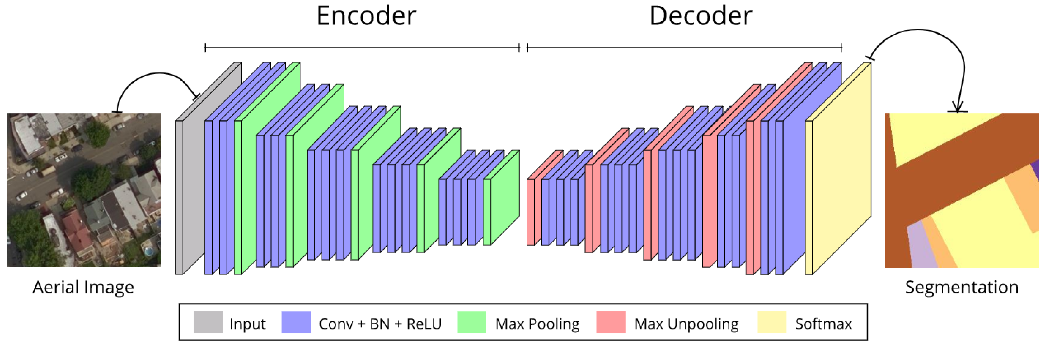
Because of the simplicity and effectiveness of SegNet on segmenting both natural and aerial images [11,42], we use it as the base network to implement pixel-level classification from aerial images and ground feature maps. The architecture of the network is illustrated in Figure 3. As we can see, the network is composed of two major components, i.e., an encoder and a decoder.
The encoder resembles the architecture of VGG-16 [35] without the fully connection layers, and it is composed of five sequential convolutional blocks. Each block in the encoder performs convolution with a trainable filter bank to produce a set of feature maps. Batch normalization [58] and element-wise rectified linear unit (ReLU) are then applied to the outputs of each convolutional layers. After convolution operation, max pooling is performed with a non-overlapping 2 by 2 window of stride 2, and thus the resulting output is subsampled by 2 times. For the first two blocks, a max pooling layer is followed after two convolutional layers (followed by batch normalization and ReLU activation), while a max pooling layer follows three convolutional layers for the rest three blocks. The encoder extracts semantic features from the original input at the cost of location information loss, with spatial resolution of input images reduced by 32 times after the processing of the encoder.
The decoder also has five convolutional blocks and its structure is symmetric to the encoder counterpart, only to use max unpooling layers to replace max pooling layers. Max unpooling is the reversed operation of max pooling, it upscales its input using memorized max pooling indices. Each block in the decoder performs max unpooling operation to upsample its input feature maps using memorized pooling indices from its corresponding encoder feature maps, and sparse feature maps are produced after the step. Then convolution is applied to densify the feature maps, with batch normalization and ReLU activation followed. The final output feature map of the decoder are recovered to the same spatial resolution as the original input, and the channel number is the same as the class number to be predicted. Finally, the output feature map is fed to a Softmax layer to make pixel-level predictions. Feeding aerial images and ground feature maps to the network respectively, then we can acquire the segmentation results, i.e., pixel-level land use classification results as required.
3.2.2. Data Fusion
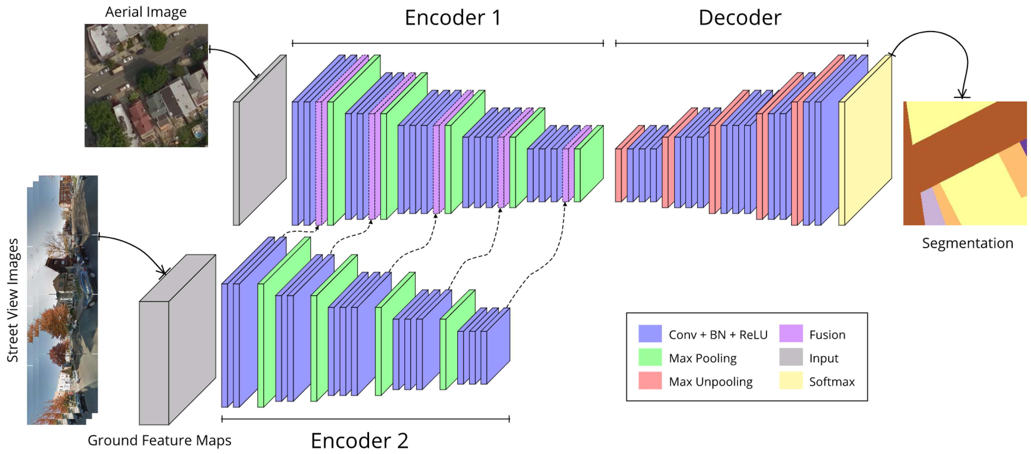
To integrate aerial images and ground feature maps together, we propose using a deep convolutional neural network-based method to fuse them, the overview of the method is shown in Figure 4. The method is based on SegNet, which is the composition of Encoder1 (without fusion layer) and Decoder (see Figure 3). However, the proposed network add an extra encoder and has a fusion strategy to fuse the two sources of data.
Encoder1 is the main branch and is designed to extract features from aerial images, while Encoder2 is used to distill features from ground feature maps. Input aerial images and ground feature maps are fed into the two encoders separately, and then the outputs from the encoders are stacked together at the fusion layer, finally fused feature maps are regarded as input fed into the decoder to upscale and make the final pixel-wise predictions.
Encoder2 also follows the structure of Encoder1, its specific structure depends on the level of fusion with block one to five respectively. The fusion can be implemented in five levels, each level corresponding to one convolutional block in Encoder2. The fusion strategy is stacking corresponding level of feature maps of Encoder1 and Encoder2. Specifically, we concatenate feature maps produced from Encoder2 to the corresponding feature maps of Encoder1 in the channel dimension as the dashed arrow indicated in Figure 4.
The encoder has the trade-off between location and semantic information, the shallow layers have more accurate location information while the deeper layers contain more comprehensive semantic information. Therefore, to find the best fusion level to balance between location accuracy and semantic representational abilities, we perform tests to stack output feature maps of the two encoders from different levels of feature maps, i.e., outputs from the five convolutional blocks of encoders without pooling operation.
4. Experiments
4.1. Dataset
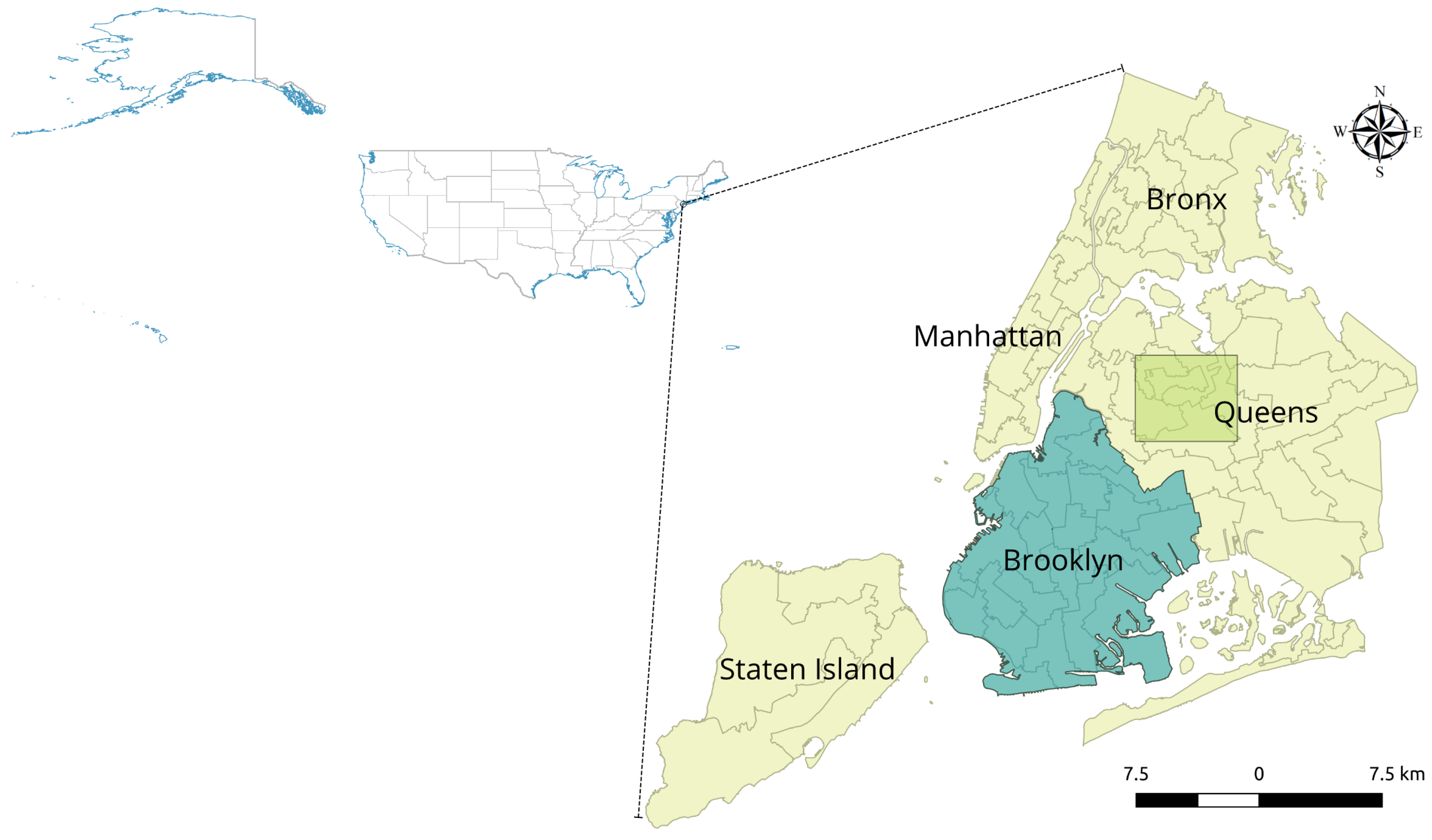
New York City (shown in Figure 5), located in the east shore of the US, is the most densely populated city in the US. It has a land area of 783.84 km with more than 8 million population. The land use of the city is highly diversified which therefore poses great challenges for land use classification. New York City consists of five boroughs, i.e., Manhattan, Brooklyn, Queens, Bronx, and Staten Island. Among them, Brooklyn borough is the most populous and Queens is the largest in land area. In our study, the major area of Brooklyn borough and a squared area of Queens borough are selected as our study area, which are highlighted in Figure 5 with different colors.
In the experiments, we use a public available dataset of New York City from [30]. The dataset consists of three types of data: high-resolution aerial images, corresponding land use maps, and sparsely sampled street view images.
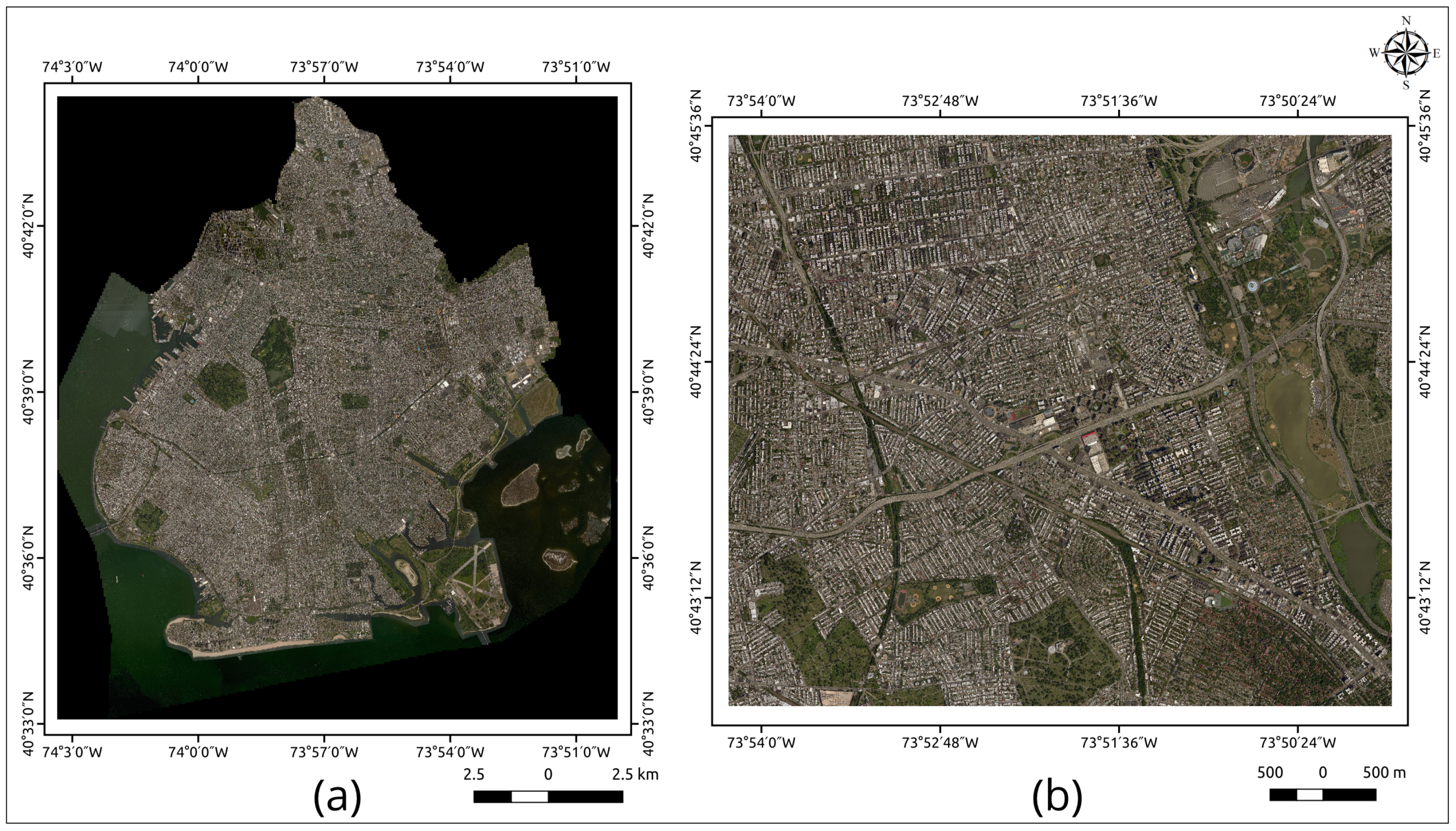
(1) Aerial images. The aerial images are from Bing Map [59] with ground resolution of about 0.3 m (as shown in Figure 6). The aerial imagery is divided into small image tiles of 256 by 256 pixels to prepare for the training and test for deep convolutional neural networks. The dataset contains two subsets. The Brooklyn dataset covers the major area of Brooklyn borough with 73,921 aerial image tiles in total. As we can see from Figure 6, a large portion of them are over water which are therefore discarded, 39,244 of them are used as training data, and 4361 randomly selected tiles are used as validation data. The Queens dataset covers a squared area in Queens borough which are used as test set, there are 10,044 aerial image tiles in total.
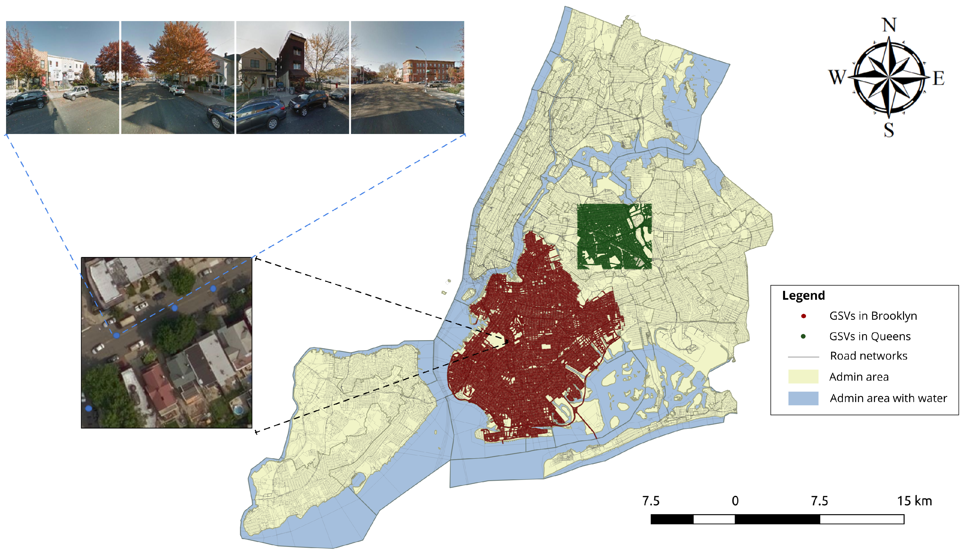
(2) Street view images. The ground-level images come from Google Street Views [60], with four images from different heading directions at each place, i.e., the north, the east, the south, and the west, and the field of view of each street view image is 90 degrees, which indicates that the panorama view of each location can be captured by the four images. The dataset we used cover Brooklyn and part of Queens borough in New York City. As we can see from Figure 7, red and green dots symbolize the locations where Google street view images are sampled in the two boroughs respectively. In Brooklyn borough, there are 139,327 locations with GSVs, four GSVs are collected in each place, the density of GSV points in this study area is 790.06 per square kilometer. In Queens area, 154,412 street view images are collected at 38,603 places, with a spatial density of points of 1167.66/km. An aerial image and its corresponding four GSVs (heading the north, the east, the south, and the west respectively) are illustrated in Figure 7.
(3) Land use maps. In this study, we use land use maps as ground truth to train and test our method. The ground truth of segmentation labels is adjusted from the GIS data of land use maps from New York City Department of City Planning [61]. The original maps are categorized into 11 categories, as shown in Table 1 with OID (original ID), documenting the primary land use in tax lot level. To accommodate the missing data and unlabeled areas, two extra categories are added, i.e., unknown and background. The adjusted land use types and corresponding descriptions (adjusted from [10]) are listed in Table 1.
4.2. Evaluation Metrics
To evaluate the pixel-level classification results, we adopt overall pixel accuracy, Kappa coefficient, mean IoU and F1 score as our evaluation metrics.
- (1)
- Pixel accuracy:
- (2)
- Kappa coefficient: , ()
- (3)
- Mean IoU: , ()
where is the ith row and jth column element in the confusion matrix, N is the total pixel numbers, and n is the number of classes.
- (4)
- F1 score:
where and are precision and recall score of class i respectively, , . measures the segmentation result of class i.
Average F1 score is the average of summed F1 scores of different categories and can measure the overall segmentation results of all the n classes.
4.3. Study on Integrating Aerial and Street View Images
To explore the effectiveness of aerial and street view images, we have conducted three groups of experiments, i.e., segmentation using aerial images only, with street view images only, and integrating aerial and street view images respectively.
- (1)
- Aerial images only. In this group of study, the input data only include aerial images, and original SegNet is used to conduct the segmentation task.
- (2)
- Street view images only. In this experiment, we first extract semantic features from GSVs, and then interpolate them in the spatial domain to acquire ground feature maps. Next, we use the spatially densified ground feature maps as inputs to SegNet by modifying the shape of input filters to match the dimensions of input ground feature maps, and finally make the dense prediction.
- (3)
- Integrating aerial and street view images. In this study, we try to fuse aerial images and ground feature maps constructed from GSVs. We use the proposed method (described in Section 3) to fuse aerial images and ground feature maps, and then acquire the final segmentation results.
4.3.1. Implementation Details
In the experiments, models are implemented based on the PyTorch [62] framework. For training phase, we use Stochastic Gradient Descend (SGD) optimization algorithm with an initial learning rate of 0.01, a momentum of 0.9, a weight decay of 0.0005, and a batch size of 16. Learning rate is divided by 10 after the epoch of 15, 25, and 35 epochs. In addition, cross entropy is used as loss function, and the encoders are initialized by VGG-16 weights pretrained on ImageNet [63], while the decoder is initialized by He initialization [64]. For street view images, we use pretrained ResNet-18 based Places-CNN [56] to extract features and set the cutoff threshold as 30 m.
4.3.2. Results
We have trained and validated the networks on Brooklyn dataset, and tested them on Queens dataset. For each group of experiment, i.e., aerial images only (aerial), street view images only (ground), and integration of the two sources of data (fused), we have trained five instances of the same network with different order of inputs since previous experiments suggest that five instances are sufficient in most cases [65], and then the average of the results on those instances of segmentation models are taken as the final results. In addition, we ignore the unknown category for the final evaluation of classification results.
Furthermore, we have experimented on fusion in different convolutional layers, the results shows that the fusion of aerial and ground feature maps matches best before the third pooling layer which indicates that the trade-off between semantic features and location information achieves the best performance in the middle. As a result, we perform the fusion before the third pooling layers in our experiments.
(1) Overall Results
We have performed three comparative experiments, the results are listed in Table 2. We can see that:
The segmentation results using overhead aerial images alone can already achieve a relatively high pixel accuracy of 77.62% and 74.02%, Kappa coefficient of 72.50% and 68.01%, and average F1 score of 61.96% and 51.86% on Brooklyn validation and Queens test sets respectively. Ground feature maps alone can reach an accuracy of 54.31% and 32.94% of pixel accuracy on the two evaluation sets, which proves that the ground feature maps constructed from GSVs contain information that can improve land use classification results. In addition, the Kappa coefficients of 40.62% and 13.15% shows that the results are fairly consistent and are better than random.
Moreover, our proposed method to fuse overhead and ground-level street view images achieves an overall accuracy of 78.10%, a Kappa coefficient of 73.10%, an average F1 score of 62.73%, and a mean IoU of 48.15% on Brooklyn validation set, which are both higher than that of using aerial images alone. Similarly, the corresponding evaluation scores (74.87%, 69.10%, 52.69%, and 39.40%) on Queens test set also witness an increase in accuracy. The improvement in the values of the evaluation metrics implies that the integration of aerial and street view images can use both the overhead and the ground-level information which help improve urban land use classification results.
In addition, our fused results of pixel accuracy (78.10% and 74.87%) have achieved better accuracy than results reported in [30] (77.40% and 70.55% on Brooklyn and Queens evaluation sets respectively). Besides, the results are also improved significantly in mean IoU, with 48.15% and 39.40% compared with 45.54% and 33.48% in [30].
It is interesting to note that the standard deviation of evaluation results are relatively small with most of the values less than 1% which indicates that the results are statistically stable. In general, the standard deviations of overall metrics of fused data are higher than that of using aerial images only, which indicates that fusing aerial and street view images introduces more uncertainty than just use aerial images alone. The standard deviations of the test results are higher than that of validation results. This is reasonable since the models are selected via validation set, and therefore it is expected that the results for the validation set will be more stable than that of the test set.
It should also be noted that the overall evaluation results of average F1 score and mean IoU are noticeably different between the validation and test sets, reaching about 10% and 9% respectively. The phenomenon is associated with the difference between our training-validation and test datasets. In our study, the training-validation and test sets are in different boroughs of New York City. The training set covers the major area of Brooklyn borough and the validation set is randomly selected in the same borough, while the test set is a squared area in Queens borough. The landscapes of the adjacent two boroughs are similar; however, they also vary slightly in certain land use categories as well as buildings facades, this may explain why the neural network trained with data from one borough works on data of another borough but with reduced accuracy.
(2) Per-class Results
The overall results reflect the average accuracy of classification among all classes. In order to figure out the variation regarding different land use categories, we compare the F1 score of each class. The validation and test results of Brooklyn and Queens datasets are shown in Table 3 and Table 4 respectively. It can be seen from the tables that:
Specific land use types, such as background, one and two family buildings, and multi-family elevator buildings show significantly higher F1 scores compared with the average, which may be related to their high percentage of areas and more distinguishable physical appearances. This is consistent with the fact that, in both datasets, background class (roads, etc.) accounts for the largest portion of land, followed by easy recognizable residential areas, especially one and two family buildings which are usually low-floor villas with big gardens. On the other hand, parking facilities and vacant land show considerably lower values than the average F1 score which may be caused by the low percentage of pixel numbers of these categories.
It should also be noted that, for some categories, the evaluation results vary significantly between Brooklyn and Queens boroughs, for example, open space and outdoor recreation achieves an accuracy of more than 15% higher in Queens than that in Brooklyn, which is related to the different urban landscapes of the two areas since the area of this land use type in Queens are significantly larger than that of Brooklyn. This suggests that deep neural networks are dependent on data, and their performances may vary with different datasets.
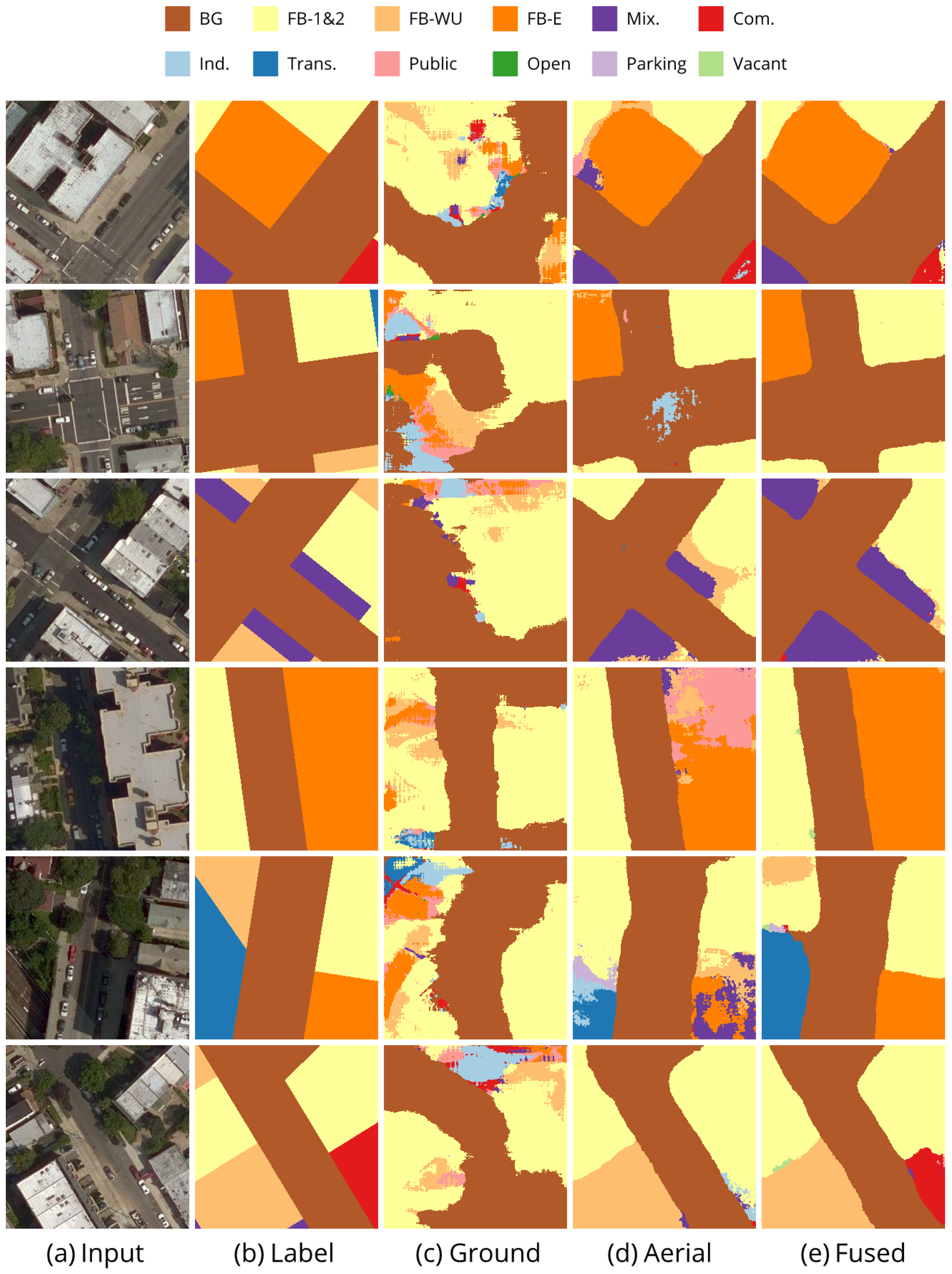
Typical examples of segmentation results of the three comparative studies are shown in Figure 8. The first three rows are the segmentation results on Brooklyn validation set, and the other three rows are results on Queens test set. As we can see, ground feature map-based segmentation is considerably distorted; however, the shape of roads is generally recovered. These results are in line with the fact that street view images are collected alone roads and streets and thus contain enough information of roads. For the results of using aerial images alone, much better results have been achieved than only use ground-level GSVs since the overall shape of the areas are better presented on aerial images. Furthermore, the fusion of ground-level information to aerial images helps to refine the segmentation results in these cases, some misclassified areas have been remedied and the results are more compacted.
4.4. Study on the Impact of Aerial Image Resolution
Although the dataset we used contains very high resolution (about 0.3 meters per pixel) aerial images, we are interested in determining whether the high resolution really benefits the pixel-level land use classification results. In addition, we also want to investigate how ground-level street view images influence the segmentation results given aerial images of different resolutions.
4.4.1. Implementation Details
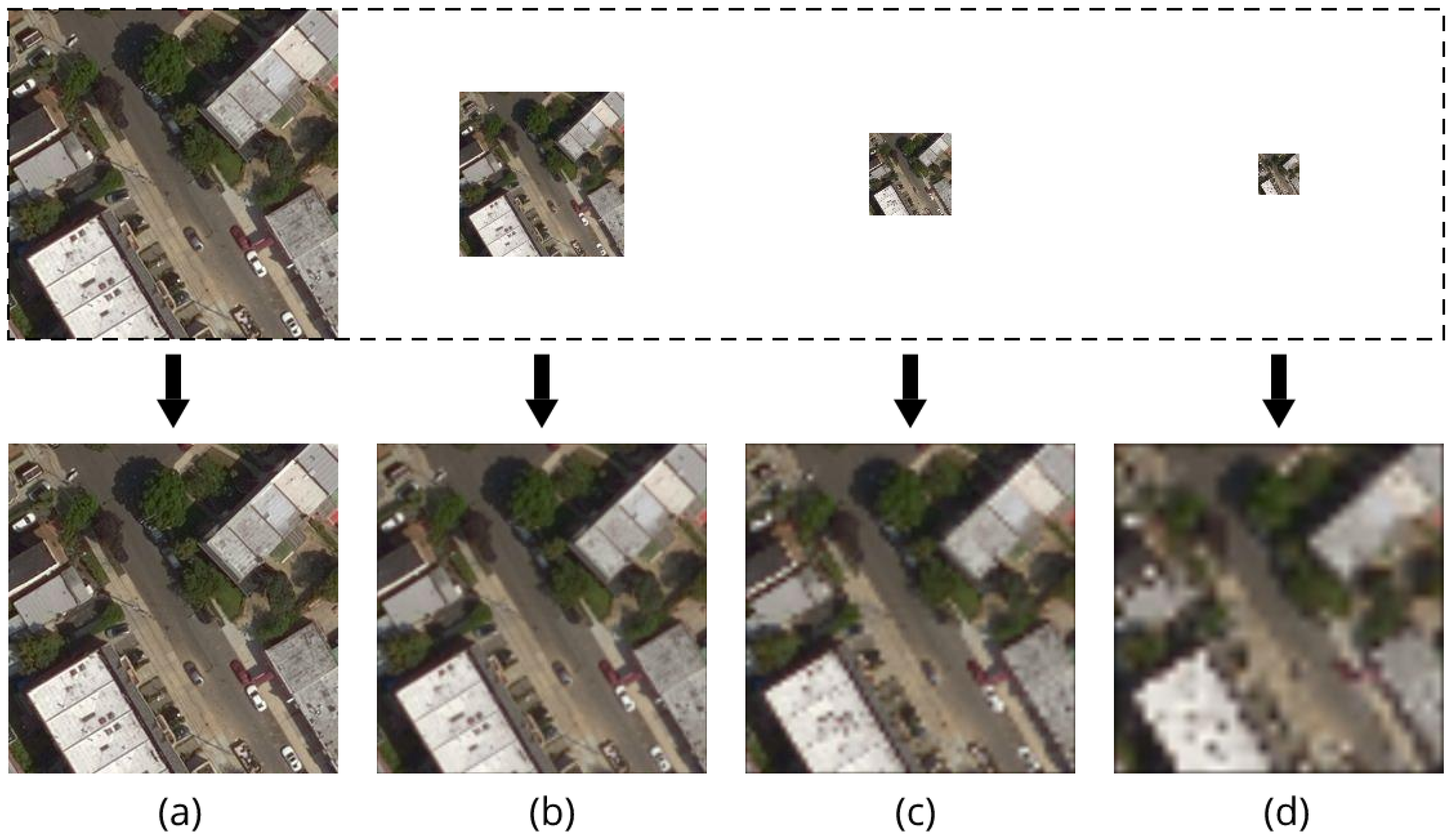
We decrease the resolution of aerial images on different levels and thus acquire an auxiliary subset of Queens test set of different image resolutions. An example of an aerial image with different resolutions are shown in Figure 9. The original aerial image tile size is 256 by 256 pixels, we firstly downsample the original image tile size by 2, 4, 8 times respectively, then lower-resolution aerial images can be acquired, i.e., 128 by 128, 64 by 64, and 32 by 32 pixels respectively as shown in Figure 9. The ground truth labels are also resized in terms of degraded sizes.
After we acquire the test set of different image resolutions, then we use them to test the pixel-level classification. Specifically, we firstly upsample the degraded images to the original size to make the images match the input size of our proposed networks. Then the resized aerial images are fed into the networks to obtain prediction results. Finally, we resize the segmentation outputs to corresponding degraded size and evaluate the final results on those resized degraded outputs.
4.4.2. Results
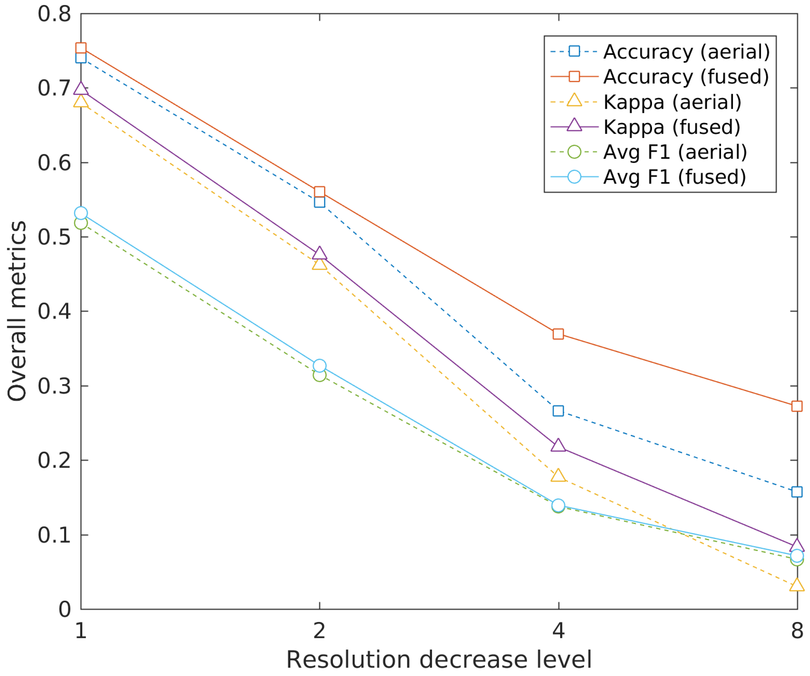
The overall evaluation metrics of prediction results using aerial images of different resolutions are shown in Figure 10. The horizontal axis is the level of resolution decrease, i.e., the factors that aerial images are downsampled from original images. The vertical axis represents the results of overall accuracy, Kappa coefficient, and average F1 score (shown in different point shapes) on the Queens test set of different resolutions. In addition, the evaluation results of using aerial images alone and integrating with street view images are shown in dashed and solid lines respectively.
As it can be seen from Figure 10, in general, the values of overall accuracy, Kappa coefficient, and average F1 score all display a similar decreasing pattern with the decline of aerial image resolutions. Furthermore, the evaluation values of using aerial and street view images together are all higher than that of using aerial images alone, regardless of resolutions. Specifically, for classification results based on aerial images only, the overall accuracy decreases with the falling of resolutions of aerial images, and the degree of decrease is dramatic with the loss of resolutions in the first two levels, this is not surprising since the details of aerial images change significantly in those levels as seen in Figure 9. The tendency is slowed down after that. For classification results based on fused data, the overall accuracy also decreases and presents a similar pattern with the situation of only aerial images used; however, the overall accuracy is higher than that of using aerial images alone. Moreover, with the help of extra ground-level information, the overall accuracy decreases slower than that of using aerial images alone, in other words, the contribution of street view images to the increase of accuracy is more significant when the resolution of aerial images is lower. Similar patterns are also observed in Kappa coefficient. Although different from that of overall accuracy and Kappa coefficient, the values of average F1 score of integrating both data are higher than that of using aerial images alone, and the increase is relatively stable with the change of aerial image resolutions.
The results indicate that aerial images with higher resolutions have better performance than images with lower resolutions in land use classification. Besides, the ground-level street view images contain useful information for the classification regardless of the resolutions of aerial images. In addition, it is interesting to note that the gap of the values of overall accuracy and Kappa coefficient of using aerial images alone and integrating both data is widen when the resolution of aerial images decreases, which implies that, in general, street view images contribute more to the increase of prediction accuracy when the aerial image resolution is lower. This is an interesting finding because the increasingly ubiquitous street view images may therefore be very useful to help better interpret many low resolution aerial or satellite images.
5. Discussion
5.1. Discussion on Classification Results
It can be seen from our experimental results that using aerial images alone can achieve a relatively high pixel-level classification accuracy, which suggests that deep neural networks have the ability to learn the mapping between different land use types and their inner spatial arrangements and patterns. Instead of selecting features manually, deep learning methods learn the representational features from given data automatically.
Furthermore, the ground feature maps constructed from street view images also include urban land use information which is proven by the prediction results of using street view images only. Thus, we have expected more improvement in accuracy when we try to integrate ground-level street view images with aerial images; however, the results are not dramatically improved despite the increase of accuracy on both validation and test set. There are several possible reasons for the results:
- (1)
- The coverage of ground-level information is limited, because the street view images are very sparsely distributed and only limited scenes near streets can be captured by the available street view images. Besides, in our study, spatial interpolation is used to project semantic information of street view images, which suffers from certain loss of information. Although cutoff distance threshold is set to limit the interpolation in local visual areas of available street view images and the weights satisfy distance decay assumption which limit noise introduced by the interpolation, the operation may still bring in certain level of noise and thus affect the final classification accuracy. In the future, better processing strategies of street view images will be further explored.
- (2)
- The base neural network we used may limit the performance of semantic segmentation results. As the focus of the present study is to investigate methods for integrating different sources of information, specifically street view images and aerial imagery, for land use classification, we choose to use SegNet because of its simple and elegant architecture, its efficiency and effectiveness in both aerial and natural image segmentation as shown in [11,42]. However, ever since the introduction of FCN, the development of DNN-based semantic segmentation networks emerge frequently. There are many alternative neural network architectures apart from SegNet can be used in the context of this work. Segmentation networks with state-of-the-art performance may well improve the accuracy of the final results in our case. It would be interesting to compare performances of different state-of-the-art CNN architectures on fusing the two sources of data in future work.
- (3)
- The two sources of data contain duplicated information, and the aerial images may already include much of what there is in the street view images. The classification results using aerial images only have achieved a relatively high accuracy, which suggests that aerial images contain most of the information for urban land use classification and the addition of street view images improve the results but not dramatically. In addition, street view images add more values when the resolutions of the aerial images are lower, which also implies that the contribution of street view images to the classification results is associated with the information provided by aerial images.
Adding street view images achieves modest improvement in average classification accuracy. This is not surprising because these images are very sparsely distributed and only available along streets. Nevertheless, we have demonstrated that they provide useful information. In the next section, we present case studies to demonstrate how street view images can help significantly improve segmentation accuracy near the street areas where they were taken.
5.2. Case Study on Segmentation Refinement
As we can see from Figure 8, the integration of GSVs refines the segmentation results of using aerial images alone. These results indicate that ground-level street view images possess useful information for land use categorization. In addition, it is interesting to note that the refinement is concentrating near the roads. The results is not surprising since those locations near roads are within the visual coverage of street view images and thus the street scenes can be captured. To go deeper into the details and investigate the effects of street view images on segmentation results, two specific cases are studied, and the street scenes and corresponding segmentation results are presented in Figure 11 and Figure 12.
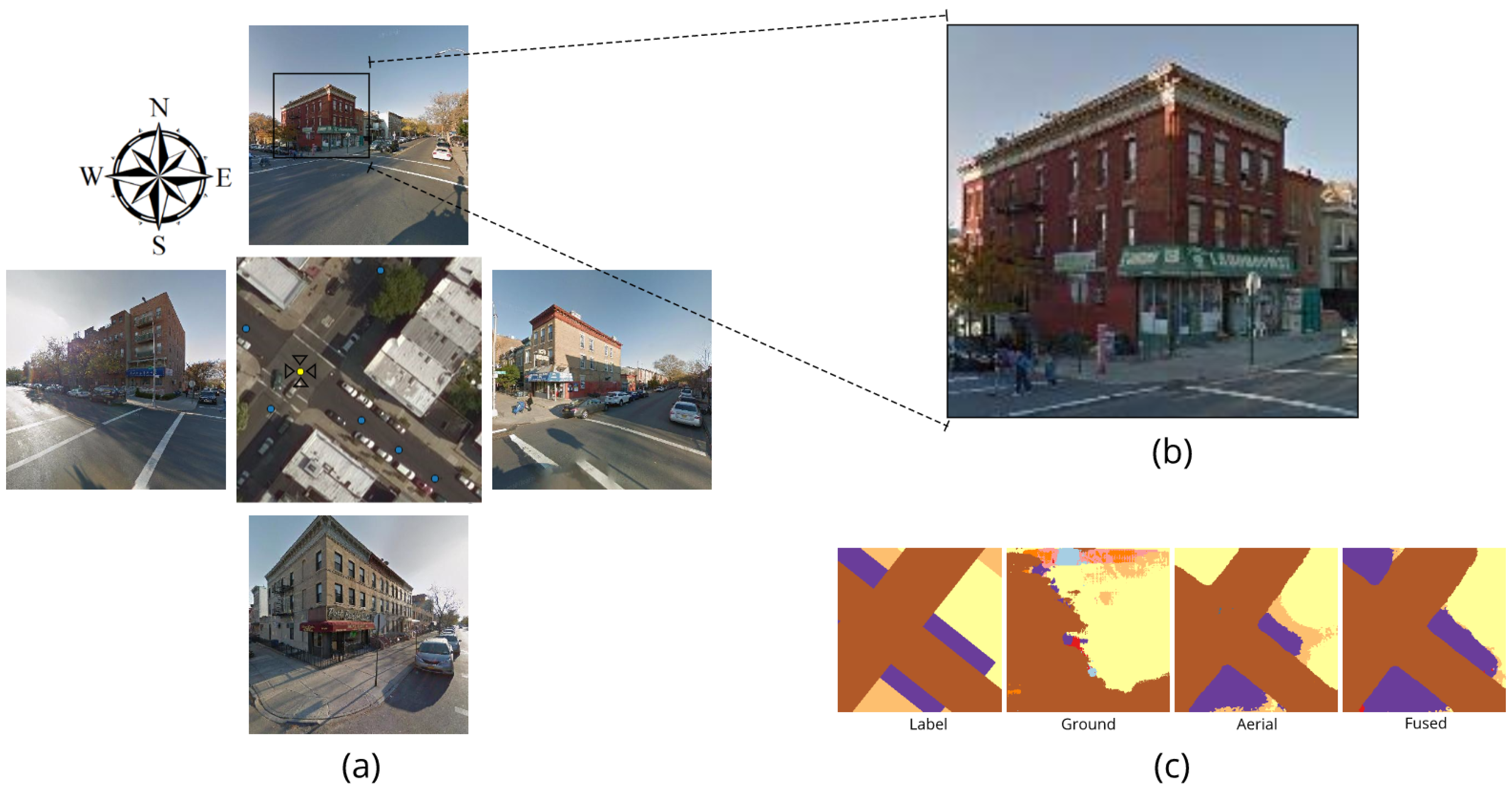
Figure 11a presents a real world scene in Brooklyn borough which is corresponding to the third row of segmentation results in Figure 8. The center is the aerial view of the area, and the blue and yellow dots are locations where GSVs are available in this study area. The surrounding four images are Google street views collected at the yellow dot location, and the orientation of the GSVs are represented by the four black hollow triangles (representing camera positions), which are heading the north, the east, the south, and the west respectively. Figure 11c shows the segmentation results of the aerial image in Figure 11a. As we can see from Figure 11a, it is difficult to tell the differences and figure out the categories of the buildings from nadir view of the aerial image. This dilemma can also be observed in the corresponding segmentation result using aerial image alone (see Figure 11c) as the categories are misclassified. However, we are able to obtain more details from the four ground-level street view images. It can be seen that the buildings nearby are three to four floors with store awnings in the first floor (as Figure 11b shows), which indicates that the buildings are typically mixed used for commercial in the ground floor and residential for upper stories. The finding is also in line with the land use map shown in Figure 11c, with the three major building areas labeled as mixed residential and commercial buildings (in purple), and the segmentation result based on integrating aerial and ground images are better than only using aerial images alone.
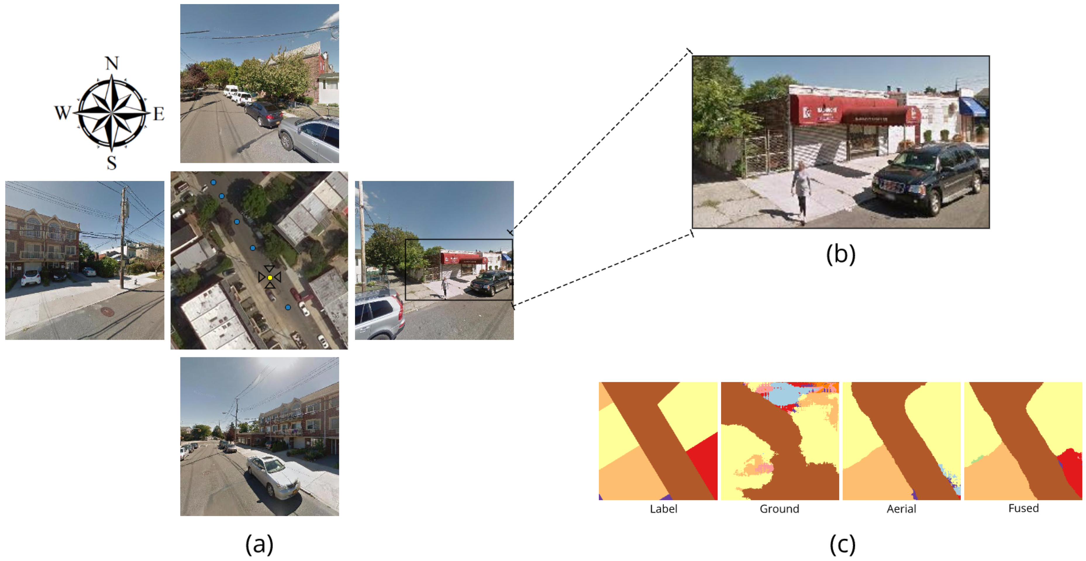
Similarly, Figure 12a presents a scene in Queens borough which is corresponding to the last row of segmentation results in Figure 8. As we can see in the aerial image, the roofs of the buildings in the overhead view are quite similar and thus it is almost indistinguishable given aerial image alone. However, we can observe great variation of building facades from the ground-level street view images. To the north, the south, and the west, the buildings in the street view images are two or three-stories buildings, which are typical walk-up residential houses or apartments. In comparison, the building shown in the street view image to the east, as Figure 12b shows, is one-floor and with two typical store awnings (one in red and the other in blue) which are easily recognized from the street view image but invisible from the aerial view. Therefore, it can be inferred that the land to the east is used for commercial purpose while the land in other directions is used for residential. This is further confirmed by the segmentation result shown in Figure 12c. We can see that the bottom-right corner of the commercial and office buildings land is misclassified as residential area when only aerial images are used; however, the segmentation result is corrected when integrating ground-level street view images.
The two case studies demonstrate that street view images can make significant contribution to improving segmentation results in the vicinity of the streets where they were taken. This therefore suggests that the major contribution of the street view images, as can be expected, may be in the visual areas that available street view images cover, rather than across a very large urban area.
6. Conclusions
Urban land use is of great significance to urban planning and management. Traditional urban land use mapping relies heavily on domain experts, which is labor-intensive and expensive. To alleviate the situation, we used a DNN-based method to label urban land in pixel level, integrating aerial images and ground-level street view images. Our method has been tested on a large publicly available dataset of New York City. The results show that it is possible to predict urban land use from very high resolution overhead images with relatively high accuracy, ground-level street view images contain useful information for land use classification, and the integration of street view images to aerial images can improve the pixel-level classification results. We have also examined the impact of aerial imagery resolution changes on land use classification, the results indicate that aerial imagery resolution is positively correlated with classification accuracy, and street view images will contribute more to enhance the classification accuracy when the resolution of aerial images is lower. Furthermore, we have discussed the limitations of the study. Specific cases of the segmentation results have also been investigated, and the case studies further demonstrate that the street view images can provide ground-level details that aerial images lack and help improve the results, especially in ambiguous situations near roads.
In the future, we plan to explore more sophisticated deep neural networks and other fusion strategies to further improve our segmentation results on fusing aerial and street view images. Although our presented methods have successfully incorporated aerial and street view images; however, there are still room to improve the pixel-level classification accuracy. We also plan to integrate more sources of proximate sensing data, such as social media data and vehicle trajectories, to further improve the land use mapping results. The combination of more sources of proximate sensing data does not just improve the urban land use mapping results, but also provides more insights for the understanding of our cities.
Author Contributions
R.C. and G.Q. conceived of the main idea; R.C., J.Z., W.T., and Q.L. developed the methodology and designed the experiments; R.C. and J.C. processed the data and conducted the experiments; R.C., B.L. and Q.Z. analyze the results. The manuscript was written by R.C. and improved by the contributions of all the co-authors.
Funding
The author acknowledges the financial support from the International Doctoral Innovation Centre, Ningbo Education Bureau, Ningbo Science and Technology Bureau, and the University of Nottingham. This work was also supported by the UK Engineering and Physical Sciences Research Council [grant number EP/L015463/1], the National Natural Science Foundation of China (No. 91546106), the Shenzhen Future Industry Development Funding Program (No. 201607281039561400), the Shenzhen Scientific Research and Development Funding Program (No. JCYJ20170818092931604), and China Scholarship Council (No. 201708440434).
Conflicts of Interest
The authors declare no conflict of interest. The founding sponsors had no role in the design of the study; in the collection, analysis, or interpretation of data; in the writing of the manuscript, nor in the decision to publish the results.
References
- Tu, W.; Hu, Z.; Li, L.; Cao, J.; Jiang, J.; Li, Q.; Li, Q. Portraying Urban Functional Zones by Coupling Remote Sensing Imagery and Human Sensing Data. Remote Sens. 2018, 10, 141. [Google Scholar] [CrossRef]
- Pacifici, F.; Chini, M.; Emery, W.J. A neural network approach using multi-scale textural metrics from very high-resolution panchromatic imagery for urban land-use classification. Remote Sens. Environ. 2009, 113, 1276–1292. [Google Scholar] [CrossRef]
- Jia, Y.; Ge, Y.; Ling, F.; Guo, X.; Wang, J.; Wang, L.; Chen, Y.; Li, X. Urban Land Use Mapping by Combining Remote Sensing Imagery and Mobile Phone Positioning Data. Remote Sens. 2018, 10, 446. [Google Scholar] [CrossRef]
- LeCun, Y.; Bengio, Y.; Hinton, G. Deep learning. Nature 2015, 521, 436–444. [Google Scholar] [CrossRef] [PubMed]
- Garcia-Garcia, A.; Orts-Escolano, S.; Oprea, S.; Villena-Martinez, V.; Garcia-Rodriguez, J. A Review on Deep Learning Techniques Applied to Semantic Segmentation. arXiv, 2017; arXiv:1704.06857. [Google Scholar]
- Zhu, X.X.; Tuia, D.; Mou, L.; Xia, G.S.; Zhang, L.; Xu, F.; Fraundorfer, F. Deep Learning in Remote Sensing: A Comprehensive Review and List of Resources. IEEE Geosci. Remote Sens. Mag. 2017, 5, 8–36. [Google Scholar] [CrossRef] [Green Version]
- Zhu, Y.; Newsam, S. Land Use Classification Using Convolutional Neural Networks Applied to Ground-level Images. In Proceedings of the 23rd SIGSPATIAL International Conference on Advances in Geographic Information Systems, Seattle, WA, USA, 3–6 November 2015; ACM: New York, NY, USA, 2015; pp. 61:1–61:4. [Google Scholar] [CrossRef]
- Lefèvre, S.; Tuia, D.; Wegner, J.D.; Produit, T.; Nassaar, A.S. Toward Seamless Multiview Scene Analysis From Satellite to Street Level. Proc. IEEE 2017, 105, 1884–1899. [Google Scholar] [CrossRef] [Green Version]
- Anguelov, D.; Dulong, C.; Filip, D.; Frueh, C.; Lafon, S.; Lyon, R.; Ogale, A.; Vincent, L.; Weaver, J. Google Street View: Capturing the World at Street Level. Computer 2010, 43, 32–38. [Google Scholar] [CrossRef]
- Zhang, W.; Li, W.; Zhang, C.; Hanink, D.M.; Li, X.; Wang, W. Parcel-based urban land use classification in megacity using airborne LiDAR, high resolution orthoimagery, and Google Street View. Comput. Environ. Urb. Syst. 2017, 64, 215–228. [Google Scholar] [CrossRef]
- Audebert, N.; Saux, B.L.; Lefèvre, S. Beyond RGB: Very high resolution urban remote sensing with multimodal deep networks. ISPRS J. Photogramm. Remote Sens. 2018, 140, 20–32. [Google Scholar] [CrossRef] [Green Version]
- Audebert, N.; Le Saux, B.; Lefèvre, S. Semantic Segmentation of Earth Observation Data Using Multimodal and Multi-scale Deep Networks. In Computer Vision—ACCV 2016; Lai, S.H., Lepetit, V., Nishino, K., Sato, Y., Eds.; Springer International Publishing: Cham, Switzerland, 2017; pp. 180–196. [Google Scholar]
- Kampffmeyer, M.; Salberg, A.B.; Jenssen, R. Semantic Segmentation of Small Objects and Modeling of Uncertainty in Urban Remote Sensing Images Using Deep Convolutional Neural Networks. In Proceedings of the 2016 IEEE Conference on Computer Vision and Pattern Recognition Workshops, Las Vegas, NV, USA, 26 June–1 July 2016; pp. 680–688. [Google Scholar] [CrossRef]
- Albert, A.; Kaur, J.; Gonzalez, M.C. Using Convolutional Networks and Satellite Imagery to Identify Patterns in Urban Environments at a Large Scale. In Proceedings of the 23rd ACM SIGKDD International Conference on Knowledge Discovery and Data Mining, Halifax, NS, Canada, 13–17 August 2017; pp. 1357–1366. [Google Scholar] [CrossRef]
- Hu, S.; Wang, L. Automated urban land-use classification with remote sensing. Int. J. Remote Sens. 2013, 34, 790–803. [Google Scholar] [CrossRef]
- Hernandez, I.E.R.; Shi, W. A Random Forests classification method for urban land-use mapping integrating spatial metrics and texture analysis. Int. J. Remote Sens. 2018, 39, 1175–1198. [Google Scholar] [CrossRef]
- Lv, Q.; Dou, Y.; Niu, X.; Xu, J.; Xu, J.; Xia, F. Urban Land Use and Land Cover Classification Using Remotely Sensed SAR Data through Deep Belief Networks. J. Sens. 2015, 2015, 538063. [Google Scholar] [CrossRef]
- Pei, T.; Sobolevsky, S.; Ratti, C.; Shaw, S.L.; Li, T.; Zhou, C. A new insight into land use classification based on aggregated mobile phone data. Int. J. Geogr. Inf. Sci. 2014, 28, 1988–2007. [Google Scholar] [CrossRef] [Green Version]
- Antoniou, V.; Fonte, C.C.; See, L.; Estima, J.; Arsanjani, J.J.; Lupia, F.; Minghini, M.; Foody, G.M.; Fritz, S. Investigating the Feasibility of Geo-Tagged Photographs as Sources of Land Cover Input Data. ISPRS Int. J. Geo-Inf. 2016, 5, 64. [Google Scholar] [CrossRef] [Green Version]
- Torres, M.; Qiu, G. Habitat image annotation with low-level features, medium-level knowledge and location information. Multimed. Syst. 2016, 22, 767–782. [Google Scholar] [CrossRef]
- Kang, J.; Körner, M.; Wang, Y.; Taubenböck, H.; Zhu, X.X. Building instance classification using street view images. ISPRS J. Photogramm. Remote Sens. 2018. [Google Scholar] [CrossRef]
- Tu, W.; Cao, J.; Yue, Y.; Shaw, S.L.; Zhou, M.; Wang, Z.; Chang, X.; Xu, Y.; Li, Q. Coupling mobile phone and social media data: A new approach to understanding urban functions and diurnal patterns. Int. J. Geogr. Inf. Sci. 2017, 31, 2331–2358. [Google Scholar] [CrossRef]
- Cao, J.; Tu, W.; Li, Q.; Zhou, M.; Cao, R. Exploring the distribution and dynamics of functional regions using mobile phone data and social media data. In Proceedings of the 14th International Conference on Computers in Urban Planning and Urban Management, Boston, MA, USA, 7–10 July 2015; pp. 264:1–264:16. [Google Scholar]
- Akhmad Nuzir, F.; Julien Dewancker, B. Dynamic Land-Use Map Based on Twitter Data. Sustainability 2017, 9, 2158. [Google Scholar] [CrossRef]
- Tu, W.; Cao, R.; Yue, Y.; Zhou, B.; Li, Q.; Li, Q. Spatial variations in urban public ridership derived from GPS trajectories and smart card data. J. Trans. Geogr. 2018, 69, 45–57. [Google Scholar] [CrossRef]
- Liu, Y.; Wang, F.; Xiao, Y.; Gao, S. Urban land uses and traffic ‘source-sink areas’: Evidence from GPS-enabled taxi data in Shanghai. Landsc. Urb. Plan. 2012, 106, 73–87. [Google Scholar] [CrossRef]
- Liu, X.; He, J.; Yao, Y.; Zhang, J.; Liang, H.; Wang, H.; Hong, Y. Classifying urban land use by integrating remote sensing and social media data. Int. J. Geogr. Inf. Sci. 2017, 31, 1675–1696. [Google Scholar] [CrossRef]
- Hu, T.; Yang, J.; Li, X.; Gong, P. Mapping Urban Land Use by Using Landsat Images and Open Social Data. Remote Sens. 2016, 8, 151. [Google Scholar] [CrossRef]
- Jendryke, M.; Balz, T.; McClure, S.C.; Liao, M. Putting people in the picture: Combining big location-based social media data and remote sensing imagery for enhanced contextual urban information in Shanghai. Comput. Environ. Urb. Syst. 2017, 62, 99–112. [Google Scholar] [CrossRef] [Green Version]
- Workman, S.; Zhai, M.; Crandall, D.J.; Jacobs, N. A Unified Model for Near and Remote Sensing. In Proceedings of the 2017 IEEE International Conference on Computer Vision, Venice, Italy, 22–29 October 2017; pp. 2707–2716. [Google Scholar] [CrossRef]
- Cao, R.; Qiu, G. Urban land use classification based on aerial and ground images. In Proceedings of the 2018 International Conference on Content-Based Multimedia Indexing, La Rochelle, France, 4–6 September 2018. [Google Scholar]
- Sakurada, K.; Okatani, T.; Kitani, K.M. Hybrid macro–micro visual analysis for city-scale state estimation. Comput. Vis. Image Underst. 2016, 146, 86–98. [Google Scholar] [CrossRef]
- Sakurada, K.; Okatani, T.; Kitani, K.M. Massive City-Scale Surface Condition Analysis Using Ground and Aerial Imagery. In Asian Conference on Computer Vision; Springer: Cham, Switzerland, 2014; pp. 49–64. [Google Scholar]
- Krizhevsky, A.; Sutskever, I.; Hinton, G.E. ImageNet Classification with Deep Convolutional Neural Networks. In Proceedings of the Advances in Neural Information Processing Systems 25: 26th Annual Conference on Neural Information Processing Systems, Lake Tahoe, NV, USA, 3–6 December 2012; pp. 1106–1114. [Google Scholar]
- Simonyan, K.; Zisserman, A. Very Deep Convolutional Networks for Large-Scale Image Recognition. arXiv, 2014; arXiv:1409.1556. [Google Scholar]
- Szegedy, C.; Liu, W.; Jia, Y.; Sermanet, P.; Reed, S.E.; Anguelov, D.; Erhan, D.; Vanhoucke, V.; Rabinovich, A. Going deeper with convolutions. In Proceedings of the IEEE Conference on Computer Vision and Pattern Recognition, CVPR 2015, Boston, MA, USA, 7–12 June 2015; pp. 1–9. [Google Scholar] [CrossRef]
- He, K.; Zhang, X.; Ren, S.; Sun, J. Deep Residual Learning for Image Recognition. arXiv, 2015; arXiv:1512.03385. [Google Scholar]
- Ren, S.; He, K.; Girshick, R.B.; Sun, J. Faster R-CNN: Towards Real-Time Object Detection with Region Proposal Networks. IEEE Trans. Pattern Anal. Mach. Intell. 2017, 39, 1137–1149. [Google Scholar] [CrossRef] [PubMed] [Green Version]
- Redmon, J.; Farhadi, A. YOLO9000: Better, Faster, Stronger. In Proceedings of the 2017 IEEE Conference on Computer Vision and Pattern Recognition, Honolulu, HI, USA, 21–26 July 2017; pp. 6517–6525. [Google Scholar] [CrossRef]
- Liu, W.; Anguelov, D.; Erhan, D.; Szegedy, C.; Reed, S.E.; Fu, C.Y.; Berg, A.C. SSD: Single Shot MultiBox Detector. In Proceedings of the 14th European Conference on Computer Vision, Amsterdam, The Netherlands, 11–14 October 2016; pp. 21–37. [Google Scholar] [CrossRef]
- Shelhamer, E.; Long, J.; Darrell, T. Fully Convolutional Networks for Semantic Segmentation. IEEE Trans. Pattern Anal. Mach. Intell. 2017, 39, 640–651. [Google Scholar] [CrossRef] [PubMed]
- Badrinarayanan, V.; Kendall, A.; Cipolla, R. SegNet: A Deep Convolutional Encoder-Decoder Architecture for Image Segmentation. IEEE Trans. Pattern Anal. Mach. Intell. 2017, 39, 2481–2495. [Google Scholar] [CrossRef] [PubMed]
- Ronneberger, O.; Fischer, P.; Brox, T. U-Net: Convolutional Networks for Biomedical Image Segmentation. In Proceedings of the 18th International Conference on Medical Image Computing and Computer-Assisted Intervention, Munich, Germany, 5–9 October 2015; pp. 234–241. [Google Scholar] [CrossRef]
- Jégou, S.; Drozdzal, M.; Vazquez, D.; Romero, A.; Bengio, Y. The One Hundred Layers Tiramisu: Fully Convolutional DenseNets for Semantic Segmentation. arXiv, 2016; arXiv:1611.09326. [Google Scholar]
- Chen, L.C.; Papandreou, G.; Kokkinos, I.; Murphy, K.; Yuille, A.L. DeepLab: Semantic Image Segmentation with Deep Convolutional Nets, Atrous Convolution, and Fully Connected CRFs. arXiv, 2016; arXiv:1606.00915. [Google Scholar] [CrossRef] [PubMed]
- Chen, L.C.; Papandreou, G.; Schroff, F.; Adam, H. Rethinking Atrous Convolution for Semantic Image Segmentation. arXiv, 2017; arXiv:1706.05587. [Google Scholar]
- Chen, L.C.; Zhu, Y.; Papandreou, G.; Schroff, F.; Adam, H. Encoder-Decoder with Atrous Separable Convolution for Semantic Image Segmentation. arXiv, 2018; arXiv:1802.02611. [Google Scholar]
- Chen, L.C.; Papandreou, G.; Kokkinos, I.; Murphy, K.; Yuille, A.L. Semantic Image Segmentation with Deep Convolutional Nets and Fully Connected CRFs. arXiv, 2014; arXiv:1412.7062. [Google Scholar]
- Liu, Y.; Fan, B.; Wang, L.; Bai, J.; Xiang, S.; Pan, C. Semantic labeling in very high resolution images via a self-cascaded convolutional neural network. ISPRS J. Photogramm. Remote Sens. 2017. [Google Scholar] [CrossRef]
- Liu, Y.; Minh Nguyen, D.; Deligiannis, N.; Ding, W.; Munteanu, A. Hourglass-ShapeNetwork Based Semantic Segmentation for High Resolution Aerial Imagery. Remote Sens. 2017, 9, 522. [Google Scholar] [CrossRef]
- Wang, H.; Wang, Y.; Zhang, Q.; Xiang, S.; Pan, C. Gated Convolutional Neural Network for Semantic Segmentation in High-Resolution Images. Remote Sens. 2017, 9, 446. [Google Scholar] [CrossRef]
- Zhang, M.; Hu, X.; Zhao, L.; Lv, Y.; Luo, M.; Pang, S. Learning Dual Multi-Scale Manifold Ranking for Semantic Segmentation of High-Resolution Images. Remote Sens. 2017, 9, 500. [Google Scholar] [CrossRef]
- ISPRS Working Group II/4. ISPRS 2D Semantic Labeling Contest. 2018. Available online: http://www2.isprs.org/commissions/comm3/wg4/semantic-labeling.html (accessed on 24 July 2018).
- Zhang, W.; Huang, H.; Schmitz, M.; Sun, X.; Wang, H.; Mayer, H. Effective Fusion of Multi-Modal Remote Sensing Data in a Fully Convolutional Network for Semantic Labeling. Remote Sens. 2017, 10, 52. [Google Scholar] [CrossRef]
- Zhang, W.; Witharana, C.; Li, W.; Zhang, C.; Li, X.; Parent, J.; Zhang, W.; Witharana, C.; Li, W.; Zhang, C.; et al. Using Deep Learning to Identify Utility Poles with Crossarms and Estimate Their Locations from Google Street View Images. Sensors 2018, 18, 2484. [Google Scholar] [CrossRef] [PubMed]
- Zhou, B.; Lapedriza, A.; Khosla, A.; Oliva, A.; Torralba, A. Places: A 10 Million Image Database for Scene Recognition. IEEE Trans. Pattern Anal. Mach. Intell. 2018, 40, 1452–1464. [Google Scholar] [CrossRef] [PubMed]
- Anjyo, K.; Lewis, J.P.; Pighin, F. Scattered Data Interpolation for Computer Graphics. In ACM SIGGRAPH 2014 Courses; ACM: New York, NY, USA, 2014; pp. 27:1–27:69. [Google Scholar]
- Ioffe, S.; Szegedy, C. Batch Normalization: Accelerating Deep Network Training by Reducing Internal Covariate Shift. In Proceedings of the 32nd International Conference on Machine Learning, Lille, France, 6–11 July 2015; pp. 448–456. [Google Scholar]
- Microsoft. Bing Maps. 2018. Available online: https://www.bing.com/maps/aerial (accessed on 24 July 2018).
- Google Developers. Developer Guide of Street View API. 2018. Available online: https://developers.google.com/maps/documentation/streetview/intro (accessed on 24 July 2018).
- Department of City Planning of New York City. BYTES of the BIG APPLE. 2018. Available online: https://www1.nyc.gov/site/planning/data-maps/open-data.page (accessed on 15 July 2018).
- PyTorch Core Team. PyTorch. 2018. Available online: https://pytorch.org (accessed on 15 July 2018).
- Deng, J.; Dong, W.; Socher, R.; Li, L.J.; Li, K.; Fei-Fei, L. ImageNet: A large-scale hierarchical image database. In Proceedings of the 2009 IEEE Conference on Computer Vision and Pattern Recognition, Miami, FL, USA, 20–25 June 2009; pp. 248–255. [Google Scholar] [CrossRef]
- He, K.; Zhang, X.; Ren, S.; Sun, J. Delving Deep into Rectifiers: Surpassing Human-Level Performance on ImageNet Classification. In Proceedings of the 2015 IEEE International Conference on Computer Vision, Santiago, Chile, 7–13 December 2015; pp. 1026–1034. [Google Scholar] [CrossRef]
- Lakshminarayanan, B.; Pritzel, A.; Blundell, C. Simple and Scalable Predictive Uncertainty Estimation using Deep Ensembles. In Proceedings of the Advances in Neural Information Processing Systems 30: 31th Annual Conference on Neural Information Processing Systems, Long Beach, CA, USA, 4–9 December 2017; pp. 6405–6416. [Google Scholar]
Figure 1.
The workflow of the proposed method.

Figure 2.
Construction of ground feature maps. (1) Semantic feature extraction; (2) Spatial interpolation.
Figure 2.
Construction of ground feature maps. (1) Semantic feature extraction; (2) Spatial interpolation.

Figure 3.
The network architecture of SegNet [42]. (Conv: convolution, BN: batch normalization, ReLU: rectified linear unit).
Figure 3.
The network architecture of SegNet [42]. (Conv: convolution, BN: batch normalization, ReLU: rectified linear unit).

Figure 4.
Overview of the proposed DNN-based method. Based on SegNet, an extra encoder is added. The aerial images and ground feature maps are fed into the two encoders separately, and then the output feature maps of a certain level of the two encoders are fused as input to the rest of the network to obtain final segmentation results.

Figure 5.
Overview of the study area in New York City, the US.

Figure 6.
Aerial imagery of the study area in (a) Brooklyn borough and (b) Queens borough.

Figure 7.
Google street views in the study area.

Figure 8.
Segmentation results of the three comparative studies. The first three rows are the evaluation results on Brooklyn validation set, and the others are results on Queens test set.
Figure 8.
Segmentation results of the three comparative studies. The first three rows are the evaluation results on Brooklyn validation set, and the others are results on Queens test set.

Figure 9.
Illustration of an aerial image with different resolutions. (a) 256 × 256; (b) 128 × 128; (c) 64 × 64; (d) 32 × 32 pixels.
Figure 9.
Illustration of an aerial image with different resolutions. (a) 256 × 256; (b) 128 × 128; (c) 64 × 64; (d) 32 × 32 pixels.

Figure 10.
Evaluation results of different aerial image resolutions.

Figure 11.
Case study on segmentation results from Brooklyn validation set. (a) Aerial and street view images; (b) Zoomed view of the building to the north; (c) Corresponding segmentation results.
Figure 11.
Case study on segmentation results from Brooklyn validation set. (a) Aerial and street view images; (b) Zoomed view of the building to the north; (c) Corresponding segmentation results.

Figure 12.
Case study on segmentation results from Queens test set. (a) Aerial and street view images; (b) Zoomed view of the building to the east; (c) Corresponding segmentation results.
Figure 12.
Case study on segmentation results from Queens test set. (a) Aerial and street view images; (b) Zoomed view of the building to the east; (c) Corresponding segmentation results.


Table 1.
Adjusted land use categories of New York City.
| ID | OID | Code | Land Use Type | Descriptions |
|---|---|---|---|---|
| 1 | - | BG | Background | Roads, water areas near the boundaries of the study areas |
| 2 | 1 | FB-1&2 | One and two family buildings | Single-family detached home, two-unit dwelling group, and duplex |
| 3 | 2 | FB-WU | Multi-family walk-up buildings | Two-flat, three-flat, four-flat, and townhouse |
| 4 | 3 | FB-E | Multi-family elevator buildings | Apartment building and apartment community |
| 5 | 4 | Mix. | Mixed residential and commercial buildings | Mixed use building for both commercial and residential use |
| 6 | 5 | Com. | Commercial and office buildings | Retail and general merchandise, shopping mall, restaurant, and entertainment |
| 7 | 6 | Ind. | Industrial and manufacturing | Manufacturing, warehousing, equipment sales and service |
| 8 | 7 | Trans. | Transportation and utility | Automobile service and multi-story car park |
| 9 | 8 | Public | Public facilities and institutions | Government services, hospital, and educational facilities |
| 10 | 9 | Open | Open space and outdoor recreation | Public parks, urban parks, recreational facilities, golf courses, and reservoir |
| 11 | 10 | Parking | Parking facilities | Outdoor parking facilities |
| 12 | 11 | Vacant | Vacant land | Areas with vacant space |
| 13 | - | Unknown | Unknown | Areas without land use labels |
Table 2.
Overall evaluation results (%).
| Ground | Aerial | Fused | ||
|---|---|---|---|---|
| Brooklyn | Accuracy | |||
| Kappa | ||||
| Avg. F1 | ||||
| mIoU | ||||
| Queens | Accuracy | |||
| Kappa | ||||
| Avg. F1 | ||||
| mIoU |
Table 3.
Per-class results on Brooklyn validation set (%).
| BG | FB-1&2 | FB-WU | FB-E | Mix. | Com. | Ind. | Trans. | Public | Open | Parking | Vacant | Avg. F1 | |
|---|---|---|---|---|---|---|---|---|---|---|---|---|---|
| Ground | 82.28 | 57.85 | 29.29 | 25.97 | 18.62 | 6.55 | 41.87 | 0.07 | 9.80 | 9.32 | 0 | 0 | 23.47 |
| Aerial | 94.89 | 84.19 | 63.54 | 77.69 | 49.58 | 52.73 | 65.95 | 64.33 | 61.87 | 62.79 | 29.22 | 36.76 | 61.96 |
| Fused | 95.09 | 84.40 | 64.36 | 78.43 | 51.18 | 54.53 | 67.50 | 64.17 | 62.11 | 63.00 | 30.33 | 37.68 | 62.73 |
Table 4.
Per-class results on Queens test set (%).
| BG | FB-1&2 | FB-WU | FB-E | Mix. | Com. | Ind. | Trans. | Public | Open | Parking | Vacant | Avg. F1 | |
|---|---|---|---|---|---|---|---|---|---|---|---|---|---|
| Ground | 62.16 | 28.29 | 12.14 | 0.81 | 2.96 | 2.13 | 7.92 | 0.03 | 1.97 | 1.48 | 0 | 0 | 9.99 |
| Aerial | 87.81 | 82.98 | 45.59 | 76.05 | 31.74 | 50.06 | 40.50 | 52.55 | 43.85 | 77.00 | 18.62 | 15.52 | 51.86 |
| Fused | 88.60 | 83.35 | 47.72 | 74.89 | 31.06 | 48.63 | 40.57 | 56.23 | 44.16 | 79.84 | 22.06 | 15.19 | 52.69 |
© 2018 by the authors. Licensee MDPI, Basel, Switzerland. This article is an open access article distributed under the terms and conditions of the Creative Commons Attribution (CC BY) license (http://creativecommons.org/licenses/by/4.0/).
Share and Cite
MDPI and ACS Style
Cao, R.; Zhu, J.; Tu, W.; Li, Q.; Cao, J.; Liu, B.; Zhang, Q.; Qiu, G. Integrating Aerial and Street View Images for Urban Land Use Classification. Remote Sens. 2018, 10, 1553. https://0-doi-org.brum.beds.ac.uk/10.3390/rs10101553
AMA Style
Cao R, Zhu J, Tu W, Li Q, Cao J, Liu B, Zhang Q, Qiu G. Integrating Aerial and Street View Images for Urban Land Use Classification. Remote Sensing. 2018; 10(10):1553. https://0-doi-org.brum.beds.ac.uk/10.3390/rs10101553
Chicago/Turabian StyleCao, Rui, Jiasong Zhu, Wei Tu, Qingquan Li, Jinzhou Cao, Bozhi Liu, Qian Zhang, and Guoping Qiu. 2018. "Integrating Aerial and Street View Images for Urban Land Use Classification" Remote Sensing 10, no. 10: 1553. https://0-doi-org.brum.beds.ac.uk/10.3390/rs10101553
Note that from the first issue of 2016, this journal uses article numbers instead of page numbers. See further details here.