Automatic Recognition of Pole-Like Objects from Mobile Laser Scanning Point Clouds


1
Institute of Remote Sensing and Geographic Information Systems, School of Earth and Space Science, Peking University, Beijing 100871, China
2
School of Land Science and Technology, China University of Geosciences, Beijing 100083, China
3
College of Geoscience and Surveying Engineering, China University of Mining and Technology, Beijing 100083, China
*
Author to whom correspondence should be addressed.
Remote Sens. 2018, 10(12), 1891; https://0-doi-org.brum.beds.ac.uk/10.3390/rs10121891
Submission received: 19 September 2018
/
Revised: 19 November 2018
/
Accepted: 22 November 2018
/
Published: 27 November 2018
(This article belongs to the Special Issue Mobile Laser Scanning)
Abstract
:Mobile Laser Scanning (MLS) point cloud data contains rich three-dimensional (3D) information on road ancillary facilities such as street lamps, traffic signs and utility poles. Automatically recognizing such information from point cloud would provide benefits for road safety inspection, ancillary facilities management and so on, and can also provide basic information support for the construction of an information city. This paper presents a method for extracting and classifying pole-like objects (PLOs) from unstructured MLS point cloud data. Firstly, point cloud is preprocessed to remove outliers, downsample and filter ground points. Then, the PLOs are extracted from the point cloud by spatial independence analysis and cylindrical or linear feature detection. Finally, the PLOs are automatically classified by 3D shape matching. The method was tested based on two point clouds with different road environments. The completeness, correctness and overall accuracy were 92.7%, 97.4% and 92.3% respectively in Data I. For Data II, that provided by International Society for Photogrammetry and Remote Sensing Working Group (ISPRS WG) III/5 was also used to test the performance of the method, and the completeness, correctness and overall accuracy were 90.5%, 97.1% and 91.3%, respectively. Experimental results illustrate that the proposed method can effectively extract and classify PLOs accurately and effectively, which also shows great potential for further applications of MLS point cloud data.
1. Introduction
The three-dimensional (3D) information of roads and ancillary facilities is the basic content of city information construction. The high-precision 3D information of roads and ancillary facilities plays an important role in road safety inspection, road facility management, maintenance and 3D city modeling [1,2,3,4]. In particular, pole-like objects (PLOs) such as street lamps, traffic signs and utility poles are important for urban planning, navigation and driving aids [5,6]. The increase of new roads and road reconstructions has resulted in a rapid renewal in the number and type of PLOs. The traditional manual methods cannot accommodate the collection of massive 3D information of PLOs. It is time consuming and increases the overall cost when managing, maintaining and updating the basic data as to road and ancillary facilities data.
Mobile Laser Scanning (MLS) system is an effective complement to the airborne laser scanner (ALS) and terrestrial laser scanner (TLS) systems [7]. MLS can continuously scan the road surface and objects on both sides of roads, thus providing detailed elements of urban model such as building facades, road surfaces and PLOs [6,8,9,10]. With the rapid growth of location-based services, PLOs are becoming increasingly significant for safe driving [3]. PLOs can provide drivers with the necessary warnings, distance and direction information for safety driving assist [8,11]. However, MLS point cloud is massive, including a variety of ground points, and it takes time and labor to manually identify PLOs [12,13]. Therefore, it is necessary to extract and classify PLOs automatically in a more efficient way.
For pole recognition from MLS point cloud, a variety of methods have been proposed. Some methods extracted the pole relying on additional data or scan line-by-line analysis. Wang, et al. [14] detected traffic signs based on the difference of reflective intensity, as the traffic signs were always painted with highly reflective materials. Lehtomäki, et al. [2] detected circles or ellipses from the scan lines, fused and classified clusters in the vertical direction. Lehtomäki, et al. [5] segmented scanning lines to find possible pole sweeps to cluster as a candidate pole, then further extracted PLO based on defined features. Yu, et al. [15] segmented point cloud into road and non-road points, followed by using a matching method to extract the street lamp from non-road points. There are also spatial analysis methods applied based on grid, voxel or super-voxel. Yadav, et al. [16] implemented a three-stage strategy to extract poles. Firstly, point cloud was grouped into 2D grids. Secondly, the point set in each grid was segmented vertically along the -axis. Lastly, the principal component analysis (PCA) was applied to detect vertical poles. Aijazi, et al. [6] voxelized point cloud by radius Nearest Neighbors (r-NN) and clustered the voxels according to point geometry features and color attributes to form super-voxels. The local features and geometric models were used to classify objects. Cabo, et al. [17] first voxelized point cloud and found a part of the pole by two-dimensional (2D) analysis, the horizontal section of the voxelized point cloud, then clustered and identified PLO based on voxel connectivity analysis. Lim and Suter [18] used discriminative conditional random fields and super-voxels for point cloud recognition by over-segmenting the original point cloud into super-voxels to reduce the number of points. Wu, et al. [19] located and extracted street lamps from MLS point cloud based on the super-voxel method, which included five steps, namely preprocessing, location, segmentation, feature extraction and classification. There are certain methods for extracting local shape features and semantic information. Rabbani and Van Den Heuvel [20] used the 2D Hough transform and 3D Hough transform to estimate the position and radius of the cylinder. Lam, et al. [21] used the random sample consensus (RANSAC) method and least squares method combined with Kalman filtering to fit plane for extraction 3D information of road, street lamp and electric wire. Pu, et al. [1] used a region growing algorithm to classify MLS point cloud into ground points and non-ground points, and then extracted traffic sign, vegetation and building facade based on semantic features (size, shape, orientation and spatial relationships). In addition, some researchers tried to extract poles by using the density of projected points (DoPP) that were obtained from raw point cloud. El-Halawany and Lichti [8] projected point cloud to a horizontal plane and segmented point cloud with high point density. The PLOs were extracted by using up-zone region growing. PLOs were classified based on its features such as height, surface normal vector and maximum normalized eigenvalue. Hu, et al. [22] used DoPP method to extract street lamps based on the prior information of street lamp height. In addition, there are some methods that used priori information and region of interest. Yan, et al. [23] detected and classified PLOs from the MLS point cloud. Firstly, ground points were removed from the original point cloud. Non-ground points were clustered by the Euclidean distance method, and prior information and shape information were used to detect the PLOs from these clusters. Secondly, random forest classifier was used to classify PLOs. Rodríguez-Cuenca, et al. [24] first selected region of interest in the preprocessing phase to reduce original points, detected PLOs by the Reed and Xiaoli [25] anomaly detection method, and then the unsupervised classification algorithm was used to classify vertical clusters into two categories: Artificial poles and trees.
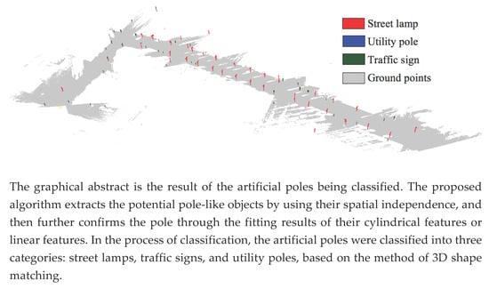
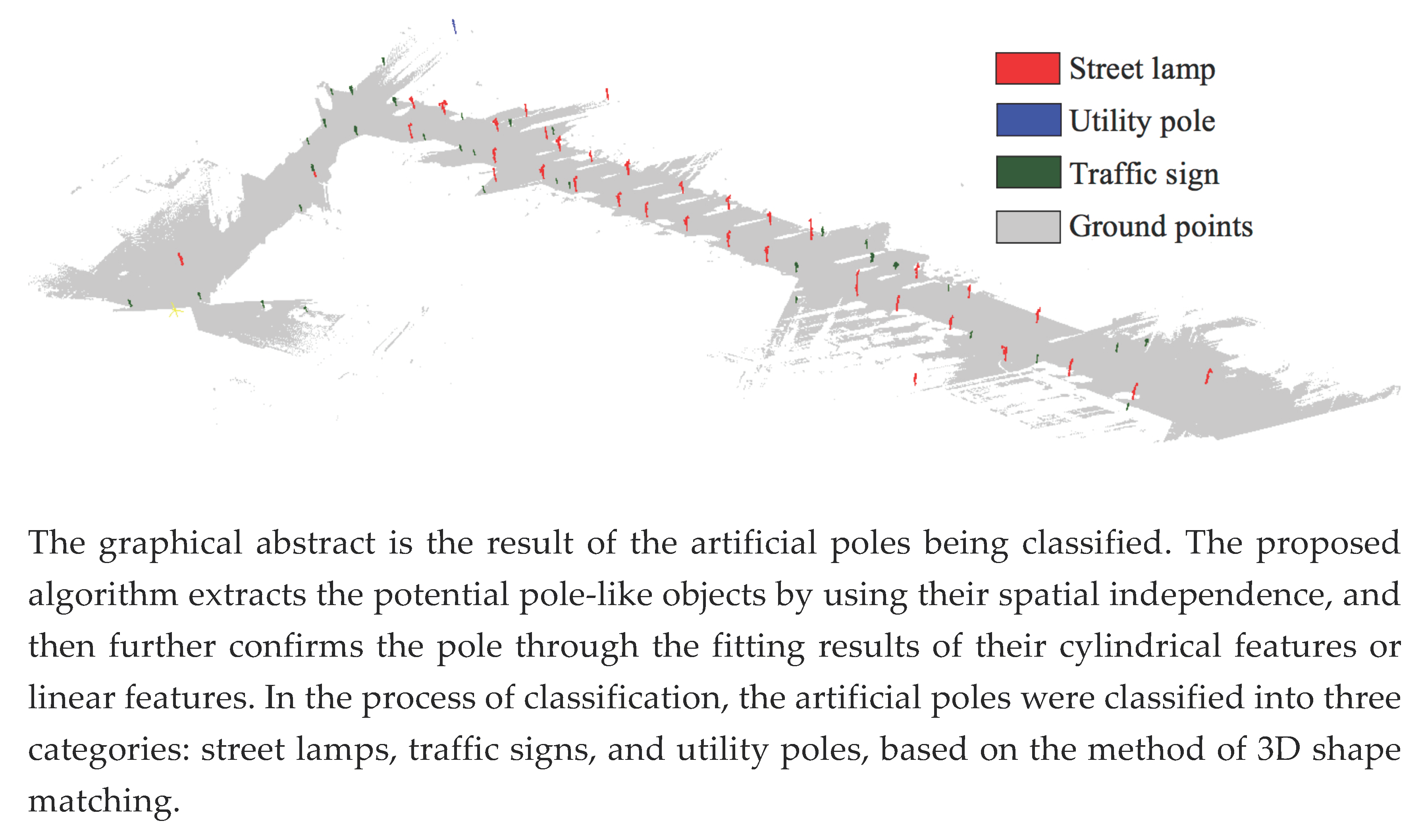
In the past decade [2,14,23,24,26,27], researchers raced to extract and classify PLOs from MLS point cloud data of urban scene and had demonstrated the effectiveness of such algorithms. However due to the complexity of the urban scene and the geometric characteristics of the PLO, some existing methods still need further improvement to improve the accuracy of extraction and classification. Some of these algorithms were subject to additional data or selection of region of interest. These algorithms of extracting the PLO could not fully use spatial and geometric (cylinder and linear) features of PLOs. Besides, these algorithms had weak classification capability since they did not take full account of classification information. To solve these problems, we propose a novel algorithm of PLO extraction and classification. Different from other algorithms, the proposed algorithm extracts the potential PLO by using their spatial independence, and then further confirms the PLO through the fitting results of their cylindrical features or linear features. In the process of classification, the street lamp with high point density and clear shape was used as the template. Compared with existing algorithms of PLO extraction and classification, the proposed algorithm has the following advantages: (1) rapidly extract the complete structure of pole. The spatial and geometric features of the pole were fully considered; (2) classify complex poles through 3D shape and height features with the template based on the method of 3D shape matching.
This paper is organized as follows. Section 1 introduces the necessity and objective of our research. Section 2 presents the proposed PLOs extraction and classification method. In Section 3 the proposed method is demonstrated and validated on two MLS point clouds of road environment. In last section, conclusions and future work are drawn.
2. Materials and Methods
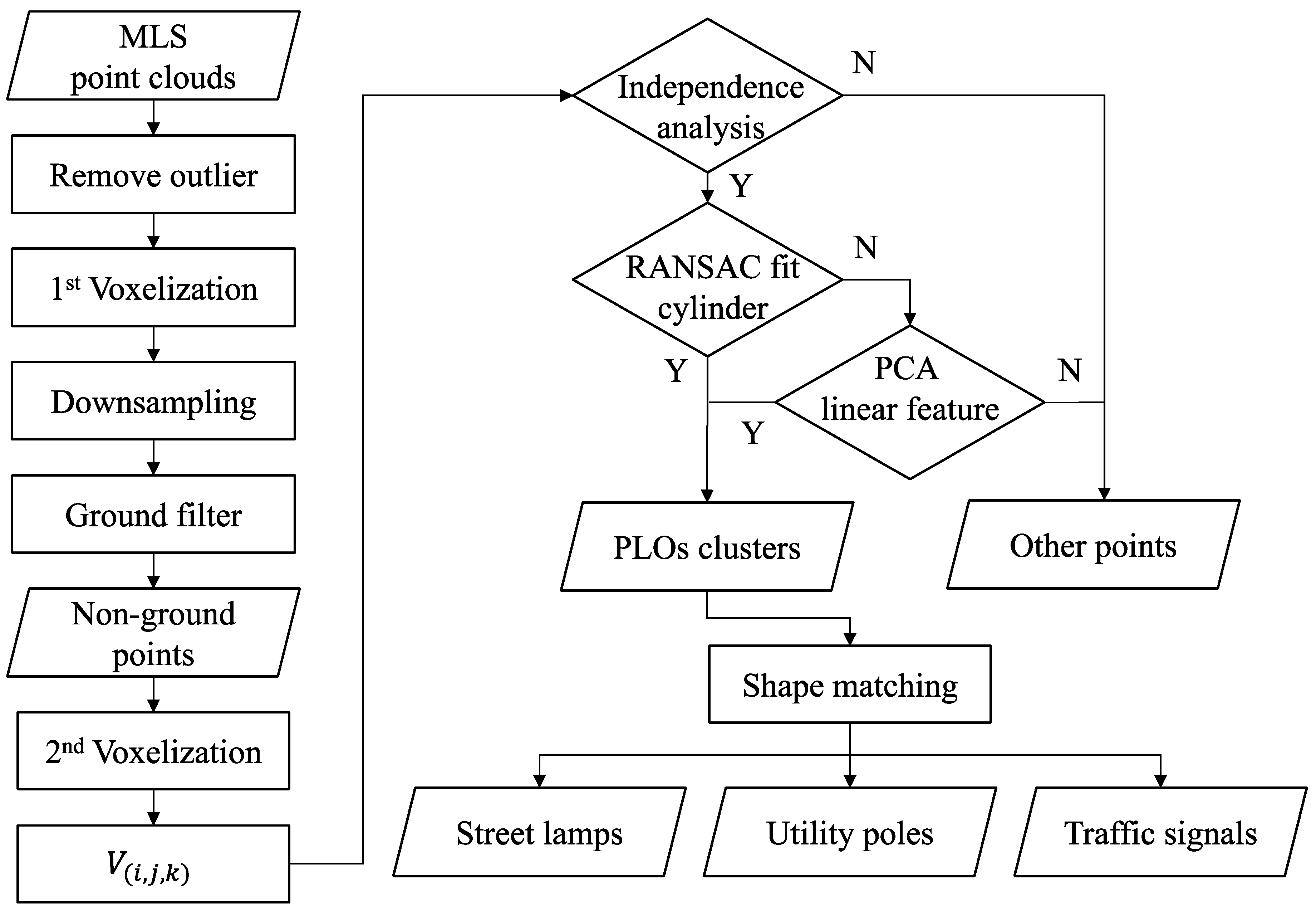
Two urban scene MLS point clouds were used to test our method. The main steps in the method are as follows (see Figure 1): (1) point cloud preprocessing, e.g., removing outliers, the first voxelization, downsampling, and ground filtering, (2) pole-like objects extraction, e.g., the second voxelization, 3D spatial independence analysis, cylindrical or linear features detection, and PLOs clusers, (3) pole-like objects classification based on 3D shape matching. These steps are described in detail in the following sections.
2.1. Mobile Laser Scanning Point Clouds
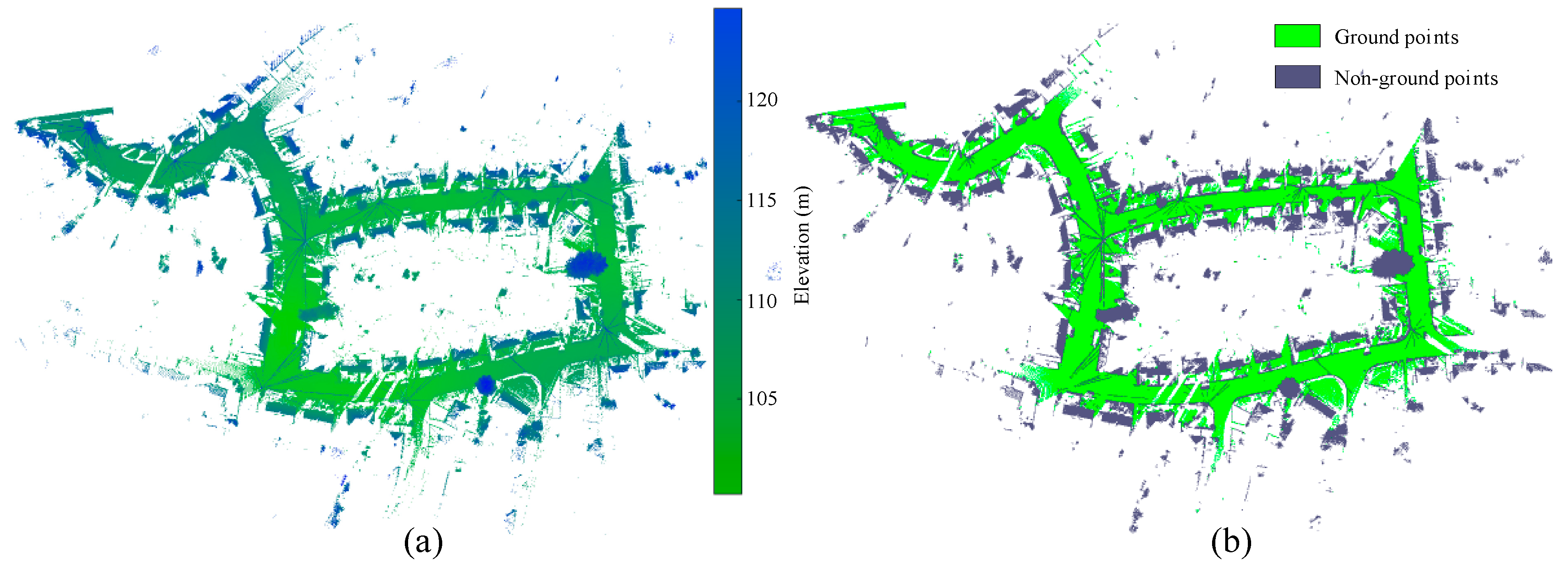
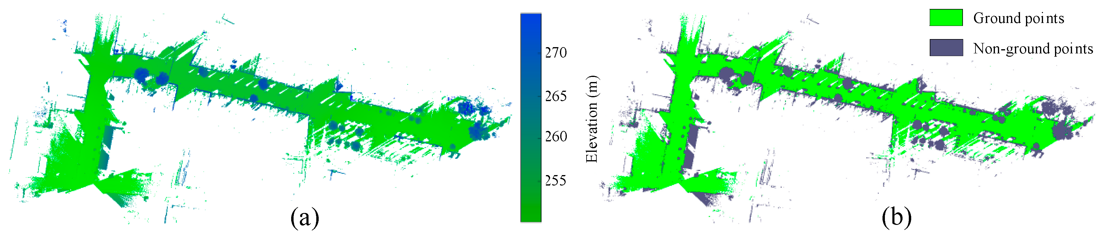
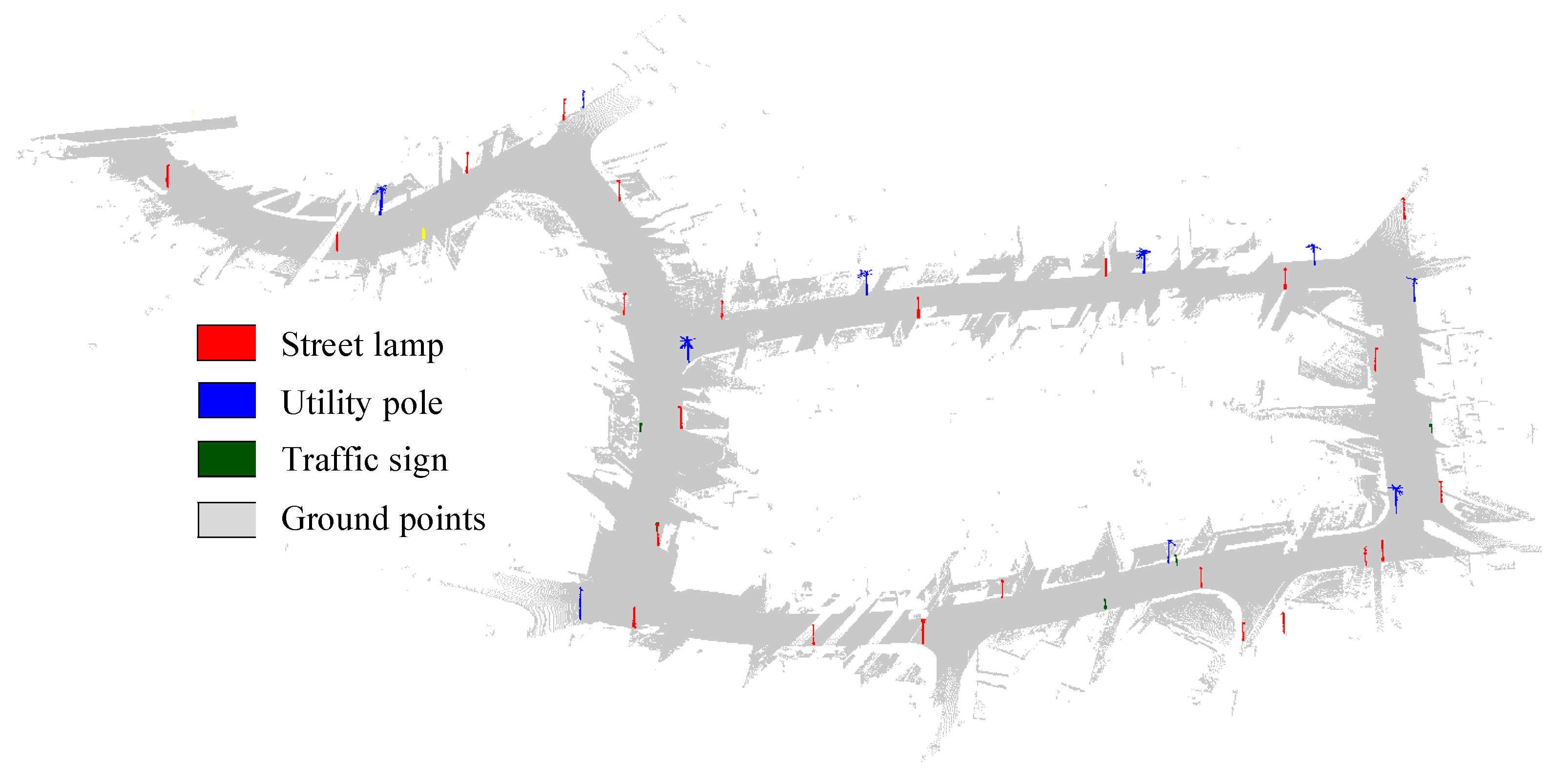
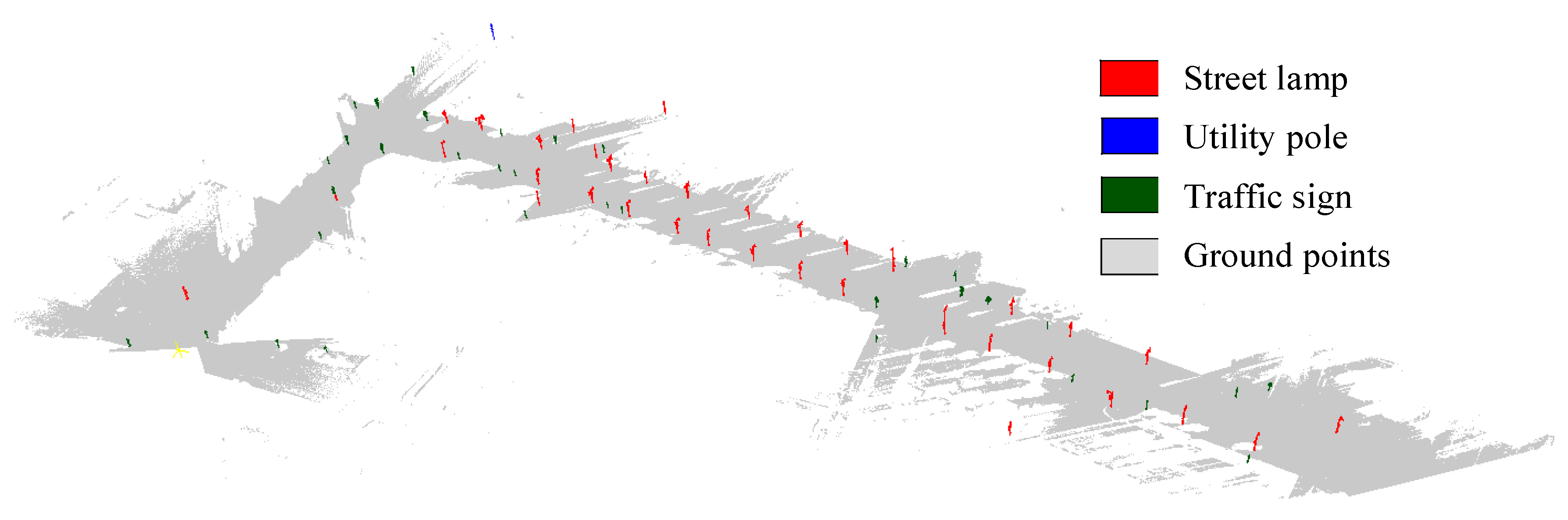
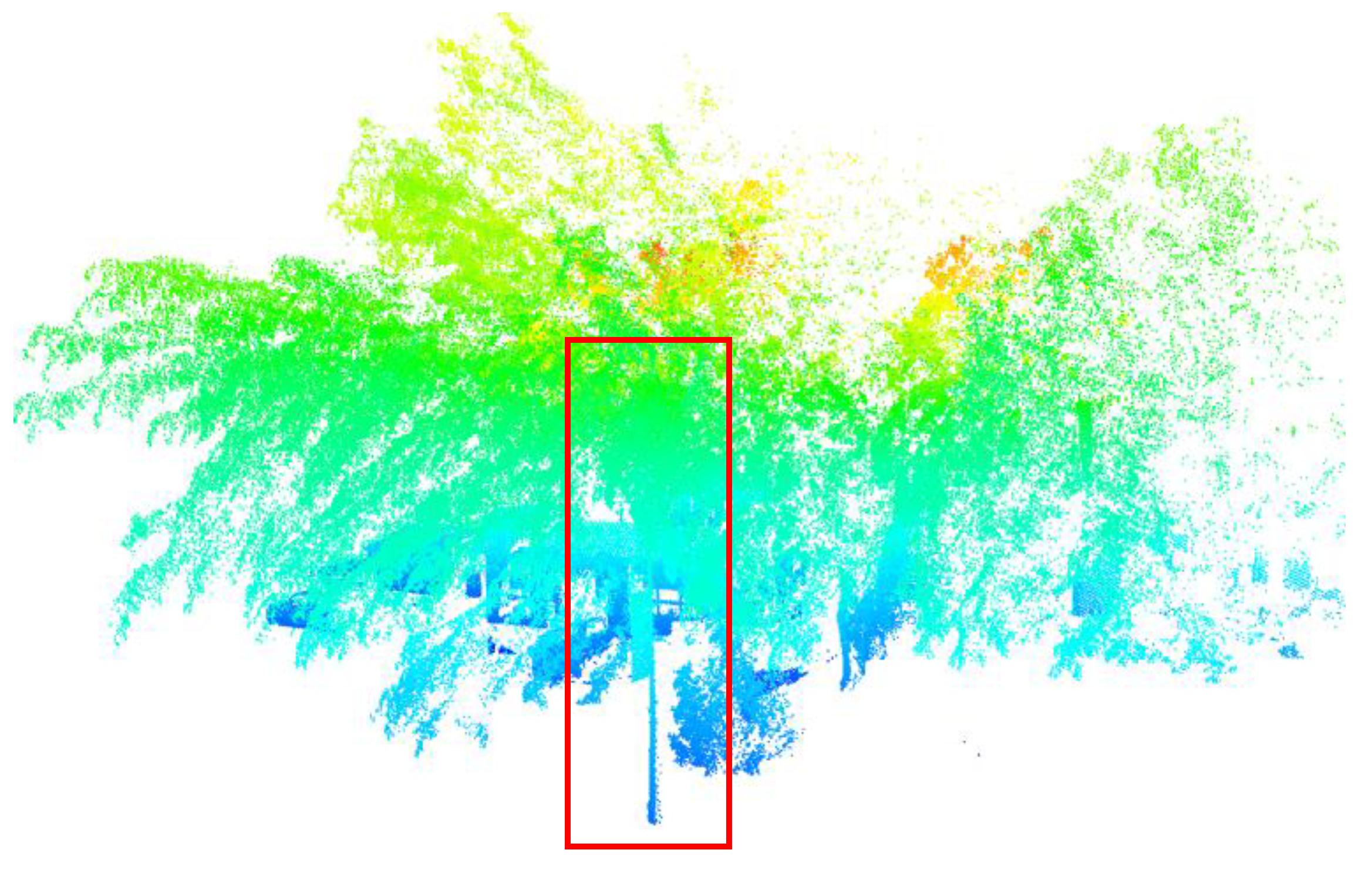
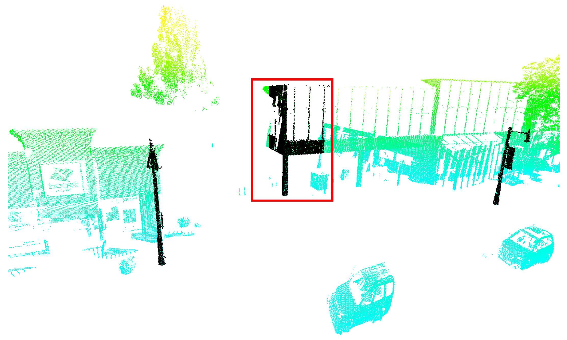
We used two MLS point clouds to evaluate the performance of the method to recognize PLOs (see Figure 2 and Figure 3). Data I is a town scene with a 651-m-long road and a data resolution of 0.037 m. Data I contains a large number of houses, street lamps, utility poles, and traffic signs, as shown in Figure 2. Data II is provided by ISPRS WG III/5 and has a 465-m-long street with average resolution of 0.015 m, as shown in Figure 3. Data II contains a wide variety of vertical objects such as street lamps, traffic signs, trees, and buildings. Table 1 shows the basic information of the two point clouds, e.g., their point density, the number of original points, points removed and non-ground points. The non-ground points of Data I after ground filtering account for 27% of the original point cloud. The non-ground points of Data II account for 21.9%. Both Data I and Data II were classified into ground points and non-ground points by filtering ground, as illustrated in Figure 2b and Figure 3b.
The manually-counted number of PLOs and categories are used to evaluate the performance of recognition method. A total of 41 reference poles were found in Data I, including 22 street lamps, 13 utility poles, 6 traffic signs and 1 other pole. Data II included a total of 74 reference poles, including 38 street lamps, 3 utility poles, 31 traffic signs and 2 other poles.
2.2. Voxelization
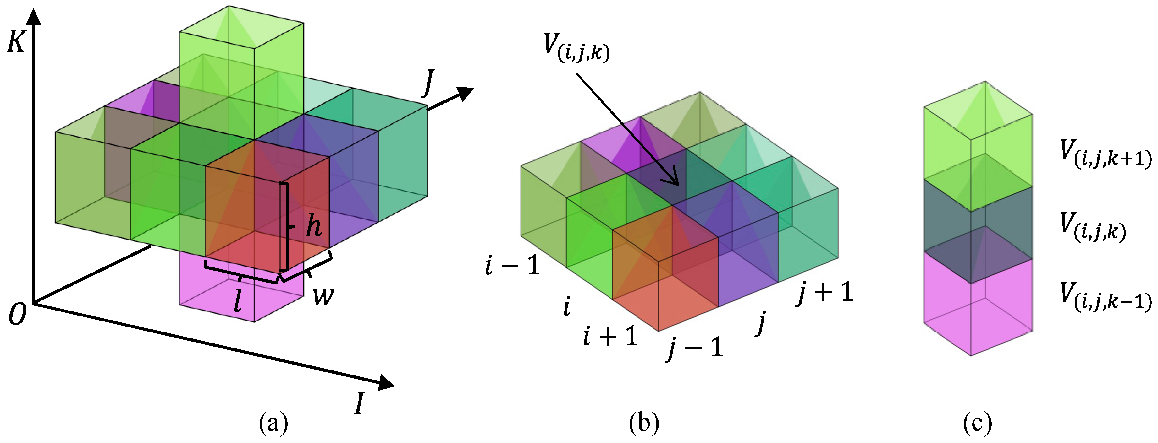
Voxel is a cube with certain length, width and height in 3D space, which is also known as spatial grid [28,29]. Voxelization is the process of grouping cluster point cloud to form cubical voxels. The computational cost of processing all points is very high. The voxelization is used to group point cloud into voxels with topological relation, which helps to improve the efficiency of the algorithm [7,30]. The relationship between central voxel and neighborhood voxels is shown in Figure 4.
In order to distinguish and index voxels, column number , row number , and layer number are illustrated in Figure 4, parallel to , and axis, respectively. Point set is indexed by corresponding coordinate of voxels. Aijazi, et al. [6] used the r-NN method to voxelize point clouds. In this paper, we convert all point cloud to voxel coordinates by the following formulas:
where is the coordinate of voxel, represents the point coordinates, are the length, width, and height of voxel, respectively, rounds a number to the next smaller integer, and is the differential coordinate value of voxel.
In our method, the voxel is designed as a small cube of the same size, which is symmetrical in 3D space. After the voxelization of point cloud, each voxel corresponds to the point set of space. Based on the coordinate index voxel and neighborhood non-empty voxels, the topological relations among voxels are established. Figure 4a illustrates the spatial relationship between central voxel and neighborhood voxels. Figure 4b shows the topological relationship among voxels in the same layer (horizontal layer), and Figure 4c represents the relationship among vertical voxels. If more neighborhood voxels of are needed, they are easily implemented based on the voxel coordinate system.
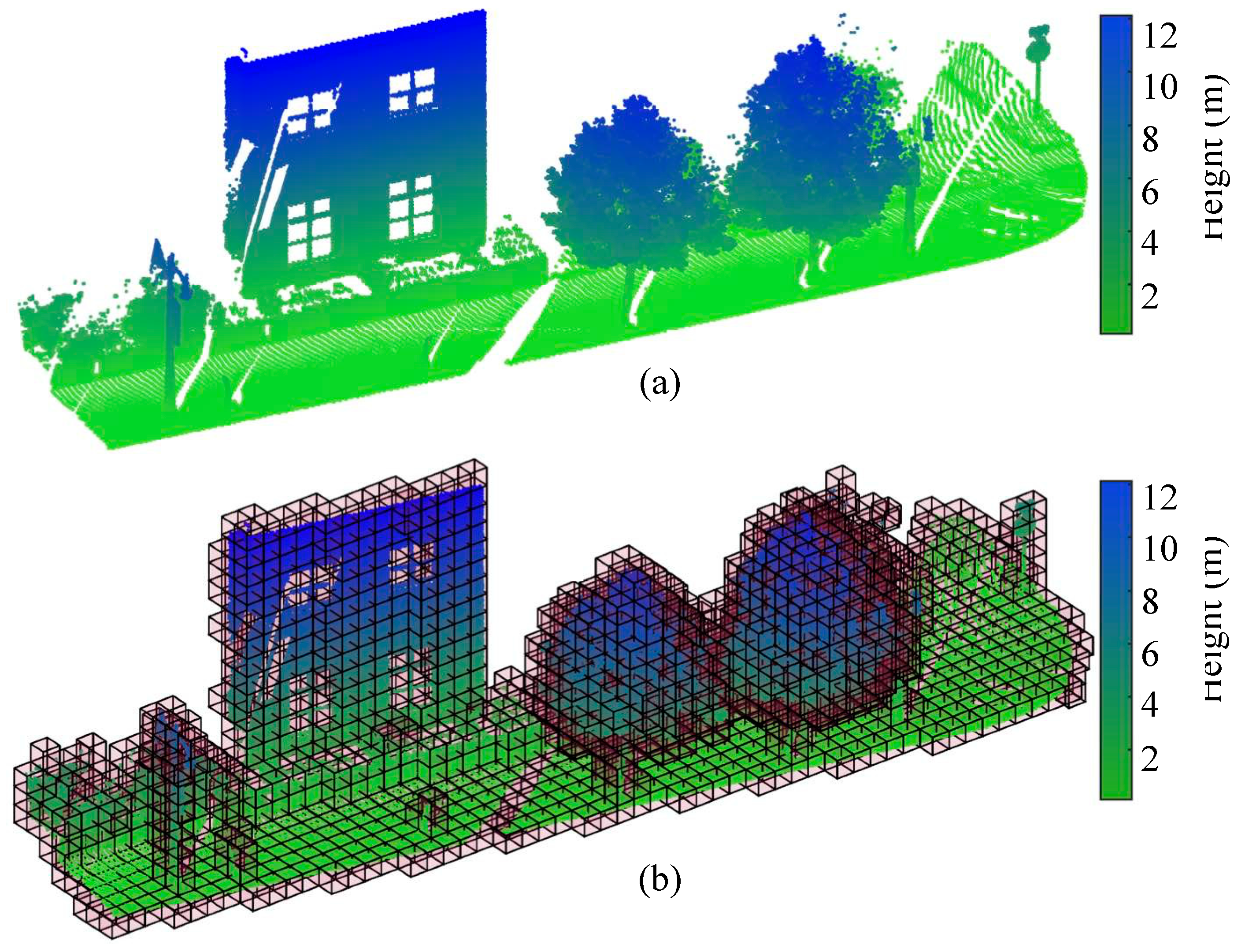
While the space size of each point cloud data is fixed, the number of voxels depends on the length of sides , and its size is determined by the average resolution of point cloud. The voxel size is fixed in the same point cloud. In our method, there are two voxelizations in the processes of downsampling and PLO detection, respectively. In the first voxelization, the average resolution of point cloud is used as the voxel size. The set of voxel size is based on the approximate diameter of the PLO during the second voxelization. Figure 5 shows the voxelization of partial point cloud.
2.3. Preprocessing
In order to improve the effectiveness and efficiency of the method, sparse outliers usually need to be removed. Point cloud downsampling is utilized before using the feature extraction method. A large number of ground points are contained in the original point cloud, while poles exists in the Non-ground points. If the ground points can be effectively removed, it will be beneficial to the poles recognition. In this section, we will perform sparse outlier removal, downsampling, and ground points filtering on the original point cloud.
2.3.1. Sparse Outlier Removal
Sparse outlier points inevitably appear in point cloud due to the influence of laser beam width and the difference of object surface properties [31,32]. These points are far away from the main point cloud. Sparse outlier points influence the local feature estimation, for example, surface normal vector or curvature, which leads to a wrong calculation [33]. By calculating the mean distance and standard deviation of the nearest neighbor points of point , the point is defined and removed as a sparse outliers if the distance to the nearest point that satisfies [34]. Here the is the distance from the -th neighbor point to the point .
There are two ways to determine the neighborhood of a point: Distance search and nearest neighbor search. In regards to the point cloud with uniform density, distance search can better represent the local geometric features. If the point cloud density varies dramatically from the scanning center, the radius search becomes impractical. Thus, the nearest neighbor search is more commonly used. In fact, it is interpreted as an adaptive search radius [35]. The original point cloud is unstructured data. In order to facilitate the neighborhood search, point cloud needs to be structured. We use the K-D tree to structure point cloud.
2.3.2. Downsampling
Due to the complexity of the road environment, MLS point cloud has different characteristics from ALS and TLS point cloud [24]. The point cloud density is affected by the driving speed as lower speed leads to higher point density. The distance between the objects and the laser scanner also affects the changing of point cloud density. The point cloud density increases while the distance between object and laser scanner decreases. And point cloud density is the highest in the road surface below the scanner. The reasonable reduction of points and maintenance structure of object are very useful to reduce the processing time of feature recognition algorithm [35]. The downsampling contains following steps, voxelize point cloud first, then calculate the center of the interior point set of voxels, and keep the point that nearest to the center. The results of the point set in the voxel is expressed only by one point.
The appropriate size of voxel directly affects the downsampling level: the larger the voxel size, the more points are removed. In order to reduce point cloud more reasonably, we establish the connection between the voxel size and the point cloud resolution. The average resolution of point cloud is taken as the size of voxel. Calculate the distance between point and point (the nearest neighbor point of point ), then summing up the distances of point pairs. The mean distance is the average resolution of point cloud. The average resolution is calculated by Formula (2).
where is the number of points in the original point cloud, is a point in point cloud, and is the closest point to , .
2.3.3. Ground Points Filtering
After the sparse outliers points are removed and downsampled, the point cloud mainly consists of ground points. These ground points include a large number of redundant points. If the ground points are effectively removed, the efficiency of subsequent detection and extraction of the PLOs is improved [36,37]. In order to filter ground points, Zhang, et al. [38] used progressive window algorithm based on the mathematical morphology ground filtering method. Vosselman [39] proposed a slope ground filtering method to identify ground points by comparing the gradients between points and their neighbors. Zheng, et al. [27] removed the ground points by piecewise elevation histogram segmentation method. Given that the ground points in a city or town are low compared with the gradient of the building and other vertical objects, it is thus more efficiently and accurately to identify the ground points by means of the cloth simulation method [40].
We used the cloth simulation method by Zhang, et al. [40] for ground points filtering. In the cloth simulation method, the LiDAR point cloud was inverted and the rigid fabric was used to cover the inverted surface. By analyzing the interaction between the distribution node and the corresponding LiDAR points, the position of the distribution node was determined to generate the approximate value of the ground. Finally, by comparing the original LiDAR points with the generated surfaces, point cloud was classified into ground points and non-ground points.
2.4. Extraction of Pole-Like Object
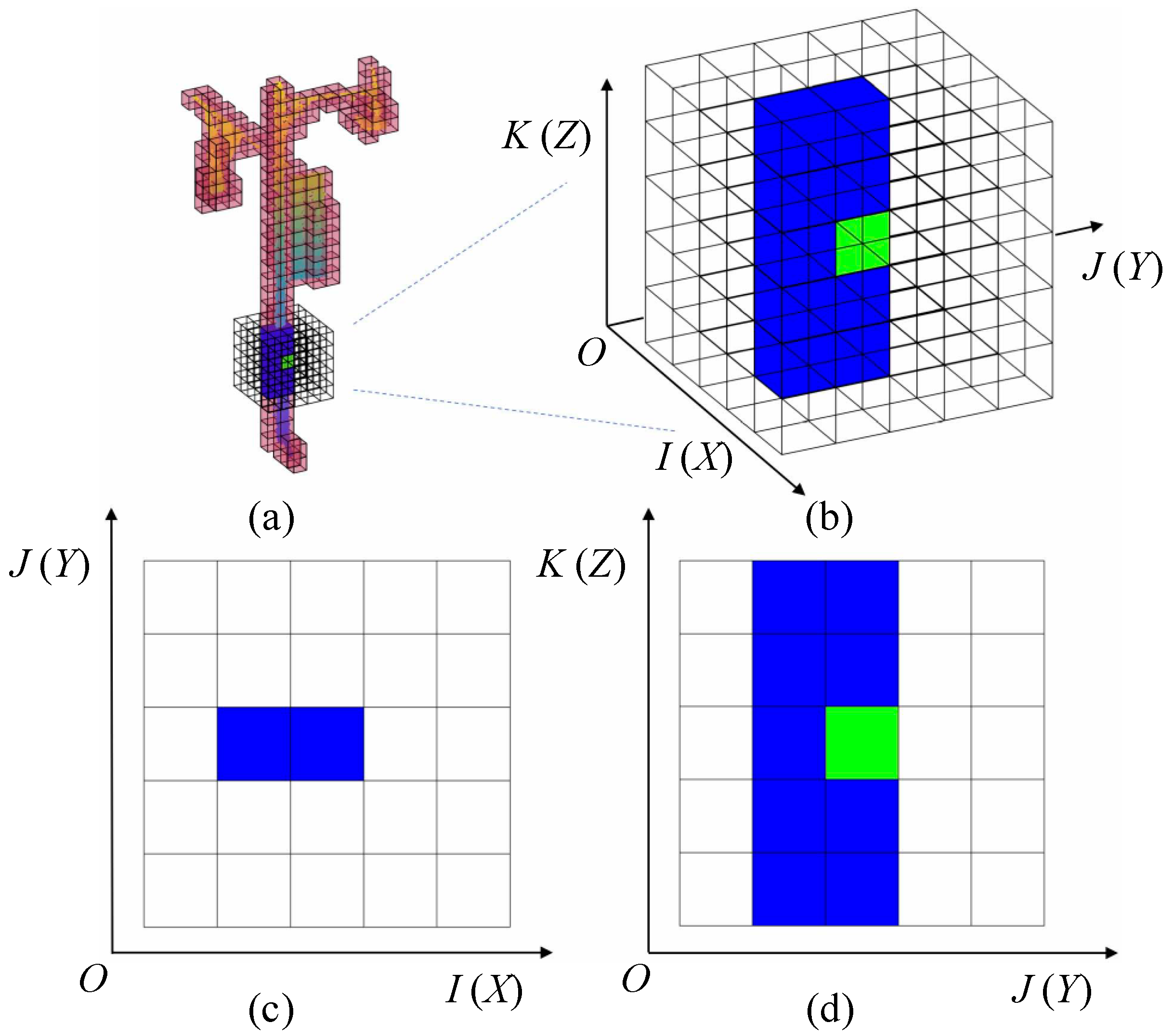
Non-ground points contain all PLOs whose structures are usually slender with different heights, diameters and perpendicular to the ground. Most road ancillary facilities include pole structure [17], and the detection of pole structure is the first step of PLO extraction. In 3D space, the PLOs are independent from other objects. The clusters of different objects could be line, plane, and volume structures. After non-ground points are voxelized, the voxels of PLO are continuous along the -axis, but discontinuous in the horizontal direction. In fact, the voxels of PLO do not exist or have fewer neighborhood non-empty voxels in the horizontal layer (the same layer). The building facade, vehicle and crown have more neighborhood non-empty voxels in multiple directions because of their large spatial volume. The voxels of PLO are quickly detected by analyzing the number of empty neighborhood voxels. To further detect the cylindrical feature or linear feature, RANSAC algorithm and PCA were used to get vertical cylinder model and principle direction of point set in neighborhood voxels. If the voxel, is one of PLO voxels, the neighborhood voxels have a smaller amount of non-empty voxels than empty voxels. Figure 6 shows different viewing angles of PLO voxels. Color-marked voxels are non-empty voxels which contain some points, and empty voxels without color are drawn to show neighborhood search. The central voxel is marked with green and the non-empty neighborhood voxels are marked with blue, as shown in Figure 6b. Figure 6c,d are the top view and side view of the neighborhood voxels, respectively. The neighborhood coordinates of voxel are, , with , and , and belonging to the set of integers. The is used to set the range of neighborhood searching. Figure 6 illustrates the searching ranges for central voxel , and the number of empty neighborhood voxels is 115.
The voxel has an independent feature if it satisfies the following three conditions: (1) voxels are non-empty voxels; (2) the outer voxels of the same layer are empty; (3) statistics on the number of empty neighborhood, voxel , must meet a certain threshold. If the voxel has this independent characteristic, then the cylindrical or linear feature of the point set in neighborhood voxels will be detected.
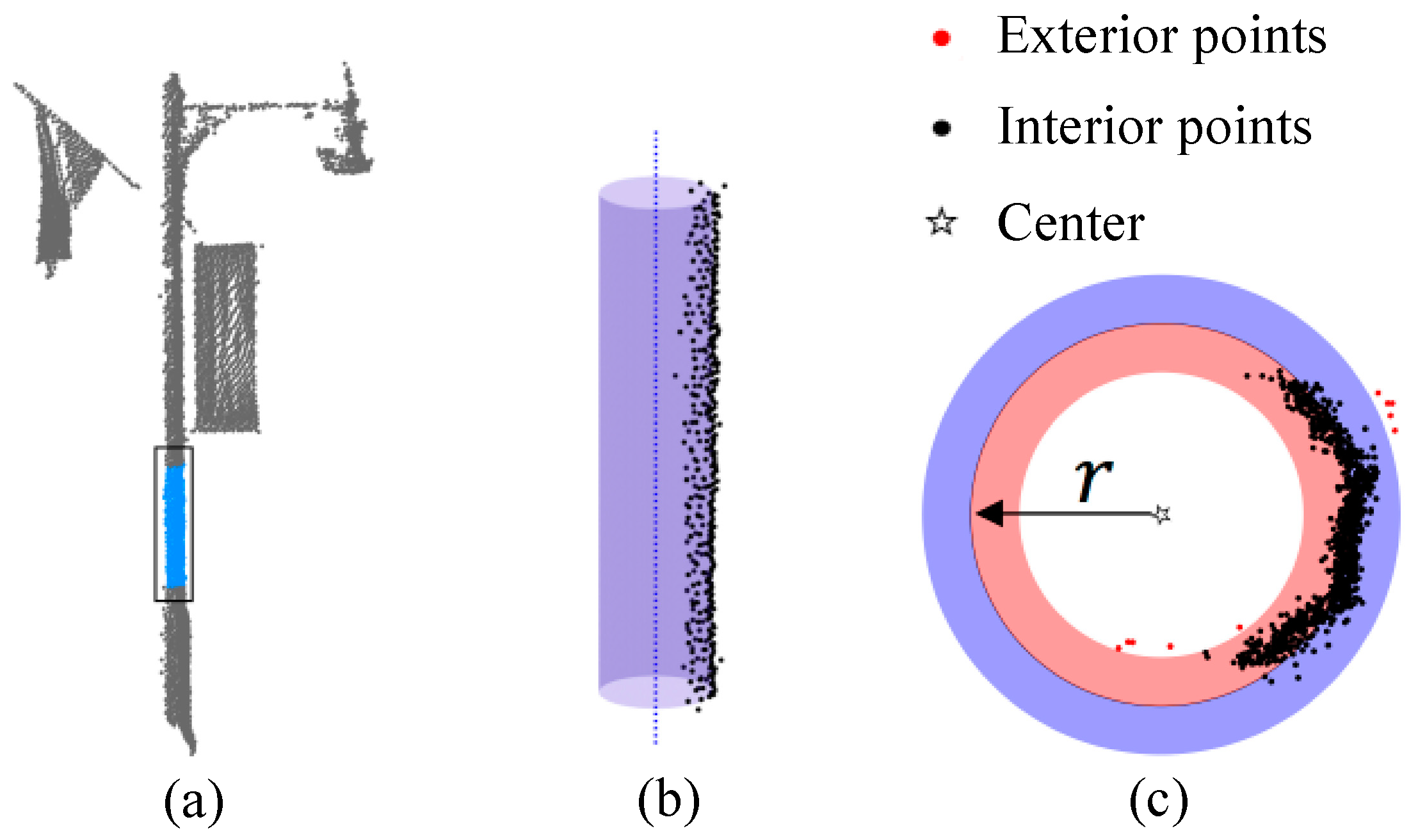
The voxels of PLOs were detected by independent analysis. If the point set belongs to pole in non-empty voxels, it has a cylindrical feature when the density of point clouds is high. The RANSAC algorithm is used to detect cylinder from point set [41,42,43]. Figure 7 shows the result of cylinder detection, and the black ring is the top view of the detected cylindrical feature. denotes the cylindrical radius and denotes distance threshold point to cylindrical surface. The blue and red regions are the regions of and , respectively. It is the interior point if the point to cylindrical surface distance satisfies , otherwise it is the exterior point. If the ratio of internal points to the number of point set is greater than or equal to 95%, it means that the point set belongs to PLO. If the point set is not adequate for detecting the cylindrical feature, it is therefore necessary to detect its linear feature.
PCA was used to detect point sets that have specific structure such as a linear feature. The eigenvalue and eigenvector represent the geometric features of the point set [35,44]. Calculate the covariance matrix of the point set, with , and () being used as the three normalized eigenvalues of . When the point set was part of a linear object, its eigenvalue , where corresponding to eigenvector is the principal direction of the linear object [26,45,46]. If the angle between vector and vector is less than 5°, the point set is a part of the PLO.
By applying to the above detection methods, it is easy to verify that voxel belongs to PLO. Region growing algorithm is used to extract the complete structure of PLO. Voxel is the initial seed and grows in the vertical direction if voxel belongs to PLO. When the neighborhood voxels of seed voxel are non-empty, they are added to the growth region. The unlabeled voxels in the growth region continue to grow as seeds until no new voxels are added to the growth region. Seed voxels are labeled in the process of growth. We limit the range of growth region to prevent overgrowth. In order to obtain a more detailed structure of PLO, the horizontal range above the voxel is set to and , and here under the voxel , only voxels with the same and coordinates are grown. At the end of the region growing, the PLO is extracted as a cluster. PLOs have a certain height and are buried on the ground. Thus, a cluster with a height less than that of the threshold is removed, and a cluster with a height above the ground and greater than that of the threshold is also removed.
2.5. Classification
The clusters of PLOs include street lamp, unity pole, traffic sign, tree and other poles. In the process of classification, the artificial PLOs will be classified into three categories: Street lamp, traffic sign, and utility pole. At this stage, the design of classifier is the key to achieving good results of recognition. The 3D shape and height of the pole are considered in the classification.
Different categories of PLO have different shapes and heights. Traffic signs, with a pole-like and plane structure, provide instructions or traffic information to road users. The shape of street lamps can be I-shaped, -shaped and T-shaped [47], and there may be banners or billboards on the poles for celebration or other purposes. Complex shapes are created by adding flags or planes to the simplest pole. The height of the PLO is an important feature that is worth considering when designing the classifier. The height of a traffic sign is usually lower than a street lamp and utility pole for observation by pedestrians and drivers. The utility pole has a power transmission function in order to avoid a connection between the electrical wires and other objects, and the height of the utility pole is usually the highest among the PLOs. The height of the street lamp is between those of the traffic sign and the utility pole.
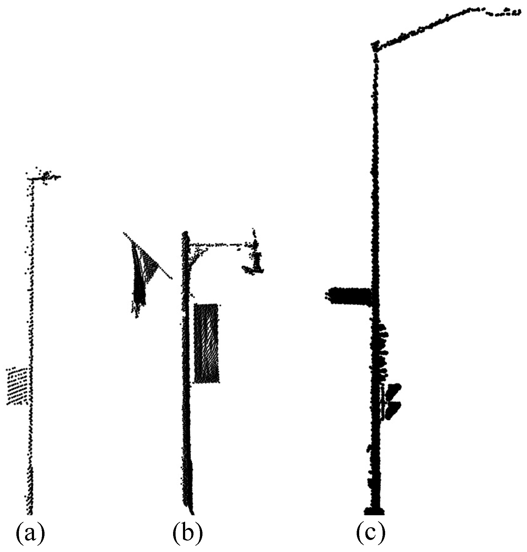
Taking into consideration the shape and height of the PLO, we chose complex street lamps as the template from original point cloud, as shown in Figure 8. The number of templates is related to the subcategory of the street lamps. The street lamp in Data I has no subcategory, so we choose a complex street lamp as Template I, as shown in Figure 8a. The street lamp in Data II has two subcategories, whose height and shape are quite different, so one of the two subcategories was chosen as Template II and Template III, respectively, as shown in Figure 8b,c. The 3D shape matching method between unclassified and template is one key problem in PLOs classification. Iterative closest point (ICP) algorithm is commonly used in the registration of 3D shapes. The ICP algorithm achieves registration by rotating and translating point set around the , , and axis, respectively [48,49]. The PLOs are perpendicular to the ground, and make principal orientation approximately parallel to the -axis. To achieve a match between unclassified pole and template, it only needs to translate the unclassified pole relative to the template and rotate around the -axis. If the root mean square error (RMSE) of 3D shape matching is less than the threshold, the unclassified pole to be matched is of the same shape of the template. The height of the PLO is also an important feature worth considering when conducting classification. If multiple templates are chosen from the same data, templates need to be prioritized through their heights. Low templates have higher priority over high templates. The unclassified poles match these templates separately, and if any pole does not belong to the street lamp category, it would be classified according to the template with the highest priority. This process would be repeated for the next unclassified object until all objects are classified. In the experiment, the priority level of Template II is higher than that of Template III. The meaning of the classification features were detailed in Table 2.
According to the above ideas, a 3D shape matching classification method is designed. and denote the unclassified pole and template, respectively. rotates around the -axis with angular resolution, and rotated point set is . Rotation matrix is calculated by Formula (3). RMSE is calculated by Formula (4). The minimum value of RMSE is the result of the 3D shape matching.
where is the angle that the turns relative to the initial position.
where is the number of points of , and represents the distance of the -th closest point pair.
According to the calculation of RMSE, the more similar the 3D shape of and , the smaller the RMSE. Therefore, RMSE is used to judge whether the shape matching is successful. Threshold is defined as the upper limit of RMSE. If the RMSE is greater than , the shape of and differ greatly and will be grouped into other objects. If the RMSE is less than or equal to , the shape of is similar to . The height difference between and needs to be further compared. If is less than or equal to the threshold , it means that and belong to the same category, namely a street lamp. If , it means that is a traffic sign, otherwise it is a utility pole.
3. Results
3.1. Parameters Setting
When the sparse outlier points were removed, the number of neighborhood points of parameter is set to 30. The size of voxel for downsampling is based on the average resolution of point cloud. During the PLOs extraction phase, the voxel size for non-ground points was set to 0.3 m. We selected the horizontal and vertical search ranges and to detect the spatial independence of voxel. Using the RANSAC algorithm to fit cylindrical feature, is set to 0.05 m. If the distance from point to cylinder surface is less than or equal to 0.05 m, the point belongs to the cylinder. After the region growing, the clusters of m and m were removed. In the ground filter based on the cloth simulation method, we set cloth resolution at 1.0 m, max iterations at 500, and classification threshold at 0.3 m. These parameters settings are suitable for most scenarios.
The shape and height of the PLOs in Data I and Data II are different, and the classification method parameters are set as shown in Table 3.
3.2. Recognition Result
In Table 4, three quality measures are listed in order to quantitatively evaluate performance of method, namely, completeness (), correctness (), and quality () [24]. They are defined as
where TP, FP and FN denote respectively the number of True-Positives, False-Positives and False-Negatives in extraction of PLOs. High indicates high detection rate of pole. indicates the correctness of poles extraction. represents the overall quality of the poles extraction.
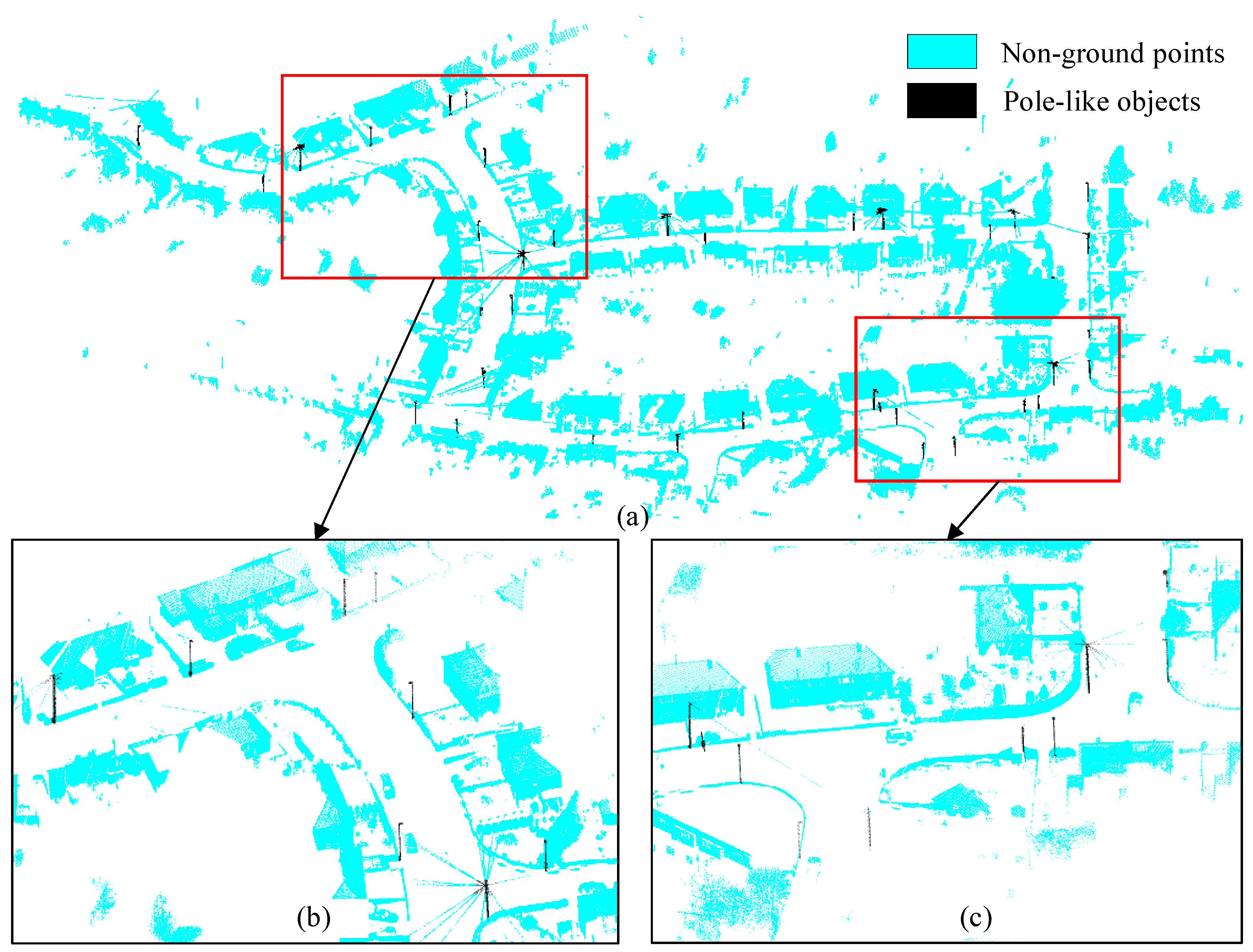
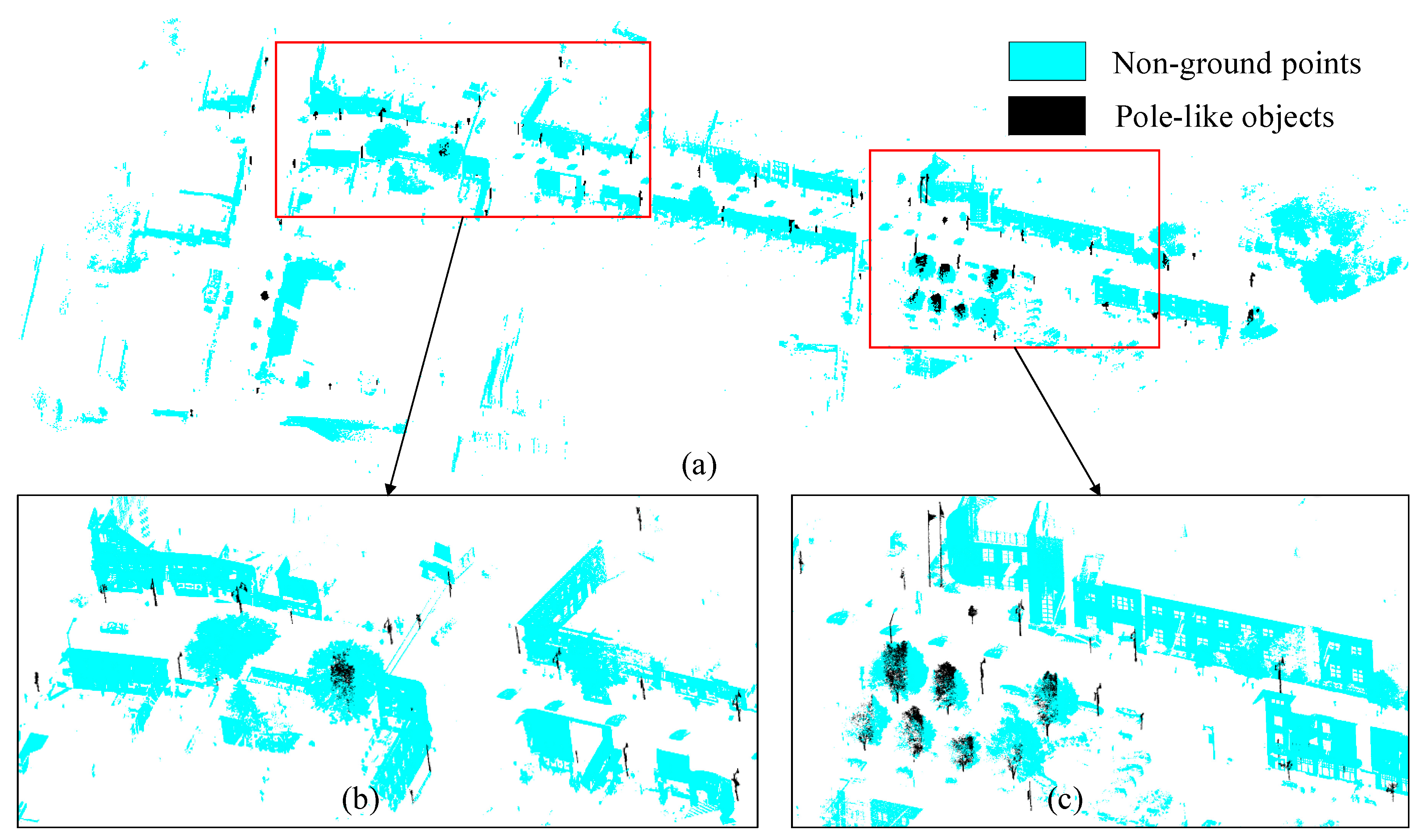
Figure 9 and Figure 10 illustrate the results of PLOs extraction of Data I and Data II, respectively. A total of 39 poles were extracted from Data I, and the number of matches with the reference poles were 38. There was 1 pole that did not match the reference poles and 3 poles were not extracted. A total of 69 poles were extracted from Data II, of which 67 poles matched the reference poles, 2 poles did not match the reference poles, and 7 poles were not extracted. The completeness, correctness and quality of the two data were calculated by Formula (5).
As performance metrics for quantitative evaluation, we use precision, overall accuracy (OA), individually for street lamp, traffic sign and utility pole. Each element of Table 5 was filled in line by line according to the classification results of PLOs. As shown in Table 5, the diagonal elements are the number of accurate classification of PLOs. The last column is the precision of the classification of the PLO. Overall accuracy was used to evaluate the overall accuracy of all three categories, which was defined as the percentage of the correct classification to the total number of extracted PLOs.
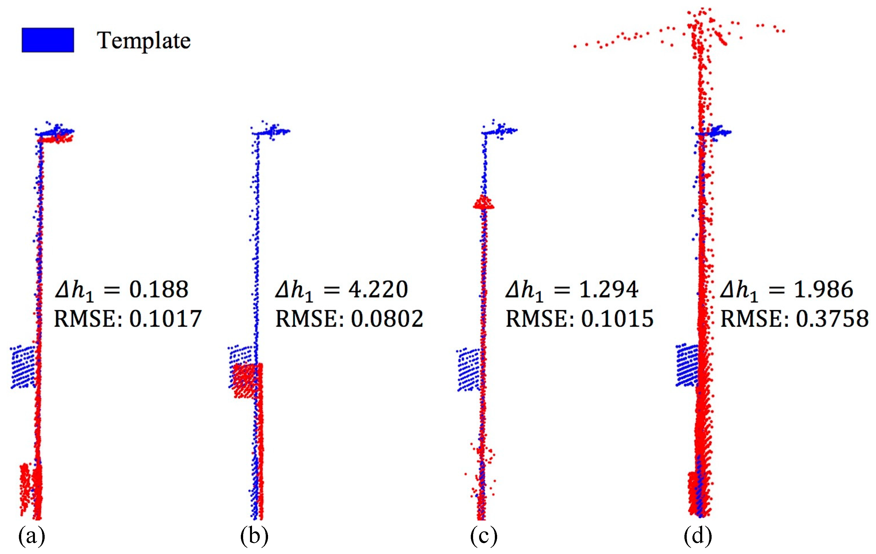
Figure 11 and Figure 12 represent the results of the 3D shape matching of the poles and the templates of Data I and Data II, respectively. The RMSE of matching results of the same category was smaller. According to Data I and Data II, PLOs had different shapes and geometric features. The height of the same category of poles was also different, as shown in Figure 11c,d. The 3D shape matching method takes into account by applying shape differences and height features to classify the PLOs. The same kind of poles match the template with small RMSE and similar height.
The road conditions of Data I was simpler than those of Data II, and the features of poles on both sides of the road were less overlapped by other objects. Figure 13 shows the result of recognition. The method had extracted 22 street lamps with a classification precision of 91.7%. The classification precision of utility poles reached 100.0%. 39 PLOs were extracted from Data I, among which were 36 correct recognitions, and the overall classification accuracy of the PLOs was 92.3%. The undetected traffic sign was highlighted as shown in Figure 13. Only one utility pole was not extracted from Data I (see Figure 14).
Figure 15 represents the result of recognition of PLOs in Data II. 35 street lamps were extracted, and the classification precision of street lamps was 92.1%. Because the utility poles are far from the road and the points are sparse, the method only correctly extracted and classified one utility pole. The classification precision of traffic signs was 93.1%. The overall classification accuracy of PLO was 91.3%.
3.3. Computational Complexity
The procedures of preprocessing, voxelization and the independence analysis were implemented in C++. The cylindrical feature fitting, linear feature detection, and shape matching processing were implemented in MATLAB. A personal computer with an Intel Core-i5-3470 2.30 GHz CPU and 8 GB of RAM was used to process Data I and Data II. The time costs of processing different steps depended on many parameters, such as the amount of input data, the complexity of algorithm, and the number of iterations. Table 6 shown a list concerning the time costs of each processing and the total time cost. The time cost of voxelization was very low. The preprocessing time for Data I and Data II were 126.3 s and 381.4 s, respectively. The original point cloud was preprocessed, which greatly reduced the amount of input data in the extraction of PLO stage. The proposed algorithm provided a promising solution for PLO recognition from MLS point cloud, and achieved acceptable computational complexity. The two data sets had a total time cost of less than half an hour, which fully proves that the proposed algorithm is highly effective and suitable for mass point cloud processing.
4. Discussion
4.1. Sensitivity Analysis
In this method, most of the parameters are configurable, and the correct selection of these parameters will affect the performance of the recognition. Parameters of preprocessing were designed for MLS point cloud and therefore these parameters were generally applicable to MLS point cloud. In the process of downsampling, the voxel size is based on the average resolution of point cloud. At the stage of PLOs extraction, the appropriate voxel size is the key to correctly extracting PLOs. The undersized voxel will reduce the efficiency of the method, and the oversized voxel will result in neighborhood voxels containing other objects. Different categories of pole can have different diameters and heights. The voxel size could be set according to the diameter of main poles, and the size should be approximate to the diameter of main poles. This ensures that neighborhood voxels of poles would be as little as possible during independence analysis, which is beneficial to the extraction of PLO. In the process of classification, the RMSE value represents the degree of similarity between template and poles. The smaller the RMSE value was, the more likely the poles was in the same category with the template. The topography, objects, and data size of Data I and Data II were different. As shown in Table 7, the mean diameters and heights of the street lamps, utility poles, and traffic signs were listed separately. The maximum gradient of Data II was greater than Data I. Data I and Data II had different characteristics, and the proposed algorithm could effectively extract and classify poles. The results show that the algorithm was insensitive to the diameter and height changes of poles.
4.2. Pole-Like Object Recognition
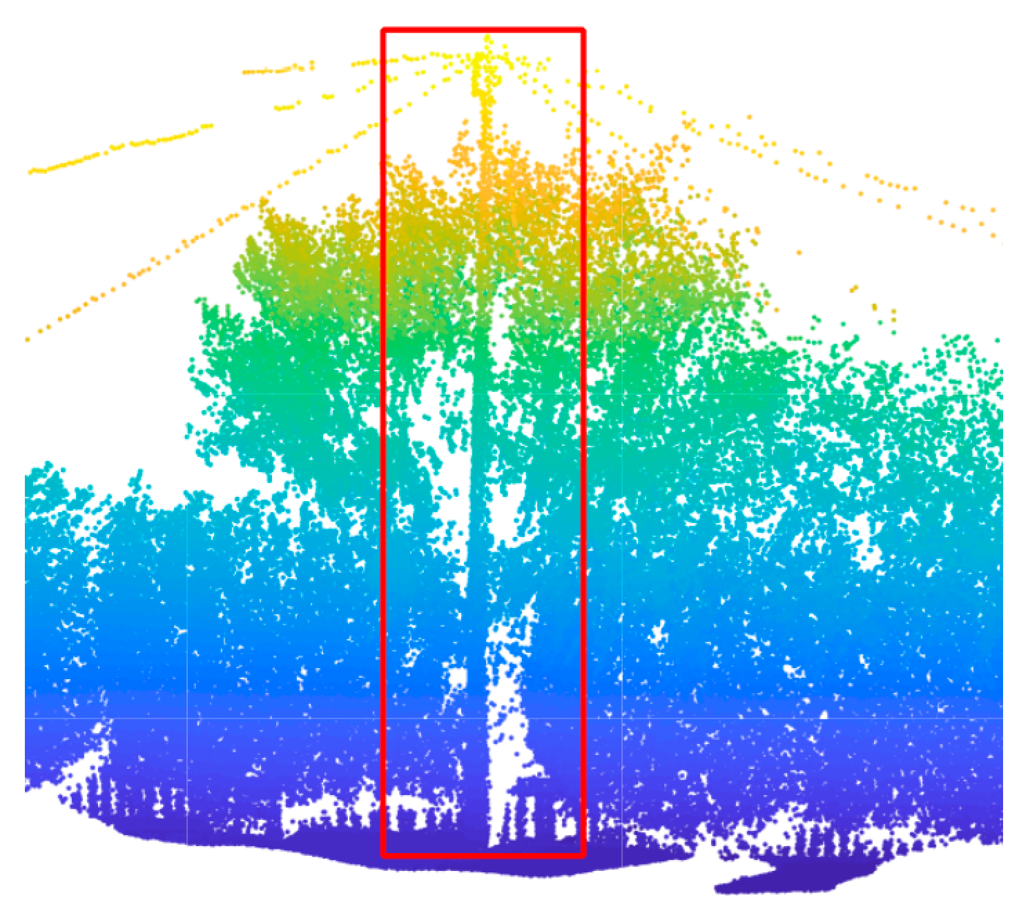
The experiments, conducted with two MLS point clouds, showed that this method can automatically extract and classify most of the PLOs. Objects overlapping and missing parts of the poles are possible challenges to accurate PLOs recognition. The utility pole is so close to the tree that it is almost surrounded by the canopy of the tree, as shown in Figure 14. Figure 16 shows an undetected street lamp, the upper part of which is surrounded by crown and the lower part is too close to the green plant. In this case of poles in the canopy, the proposed algorithm cannot recognize these poles.
Building columns and pillars between windows may lead to extraction errors (see Figure 17). These structures are spatial independence with a cylindrical or linear feature, and they were thus extracted as poles by the method. In the phase of 3D shape matching, these clusters will be classified as other objects because their values of RMSE are larger than the threshold .
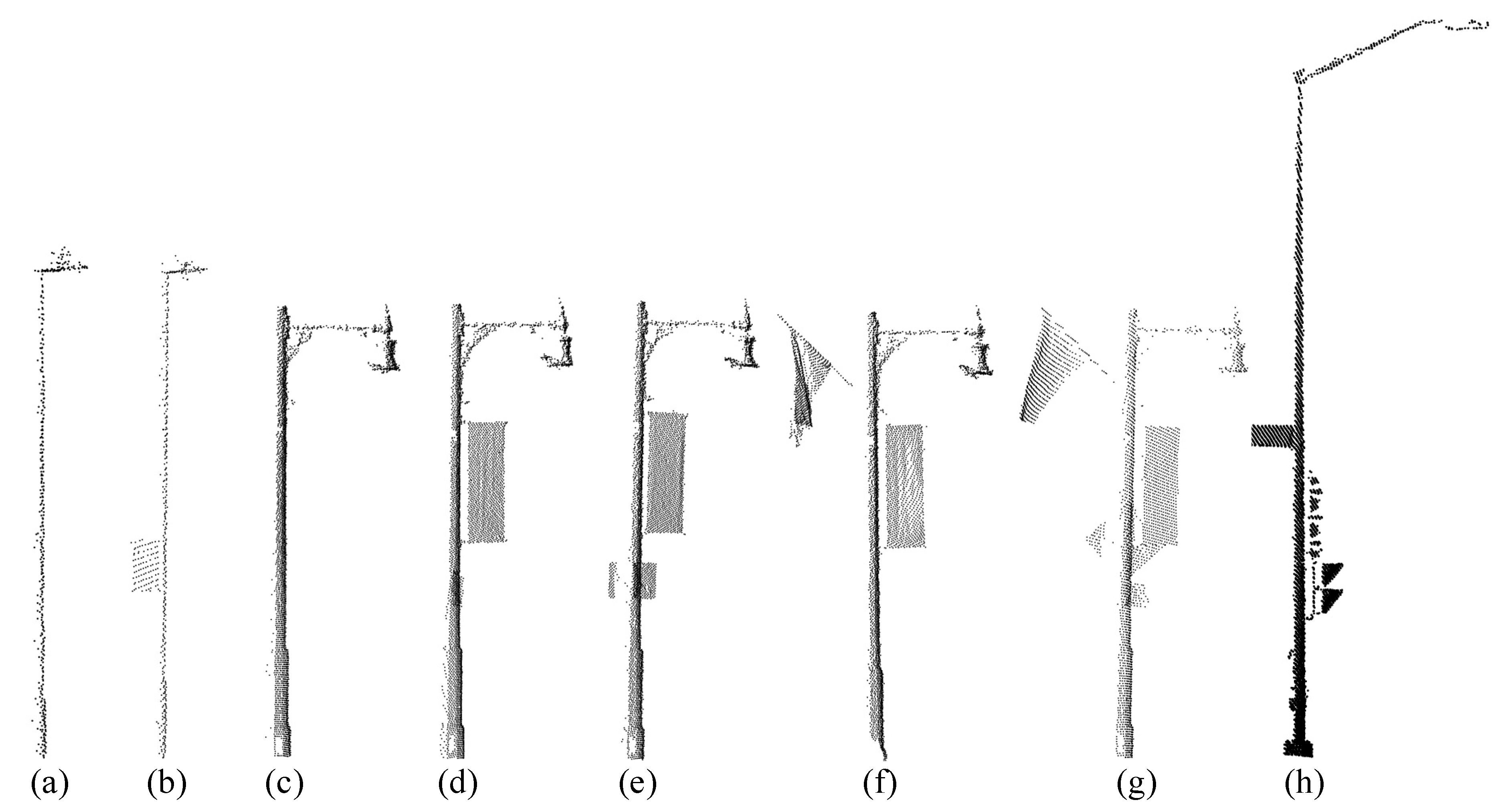
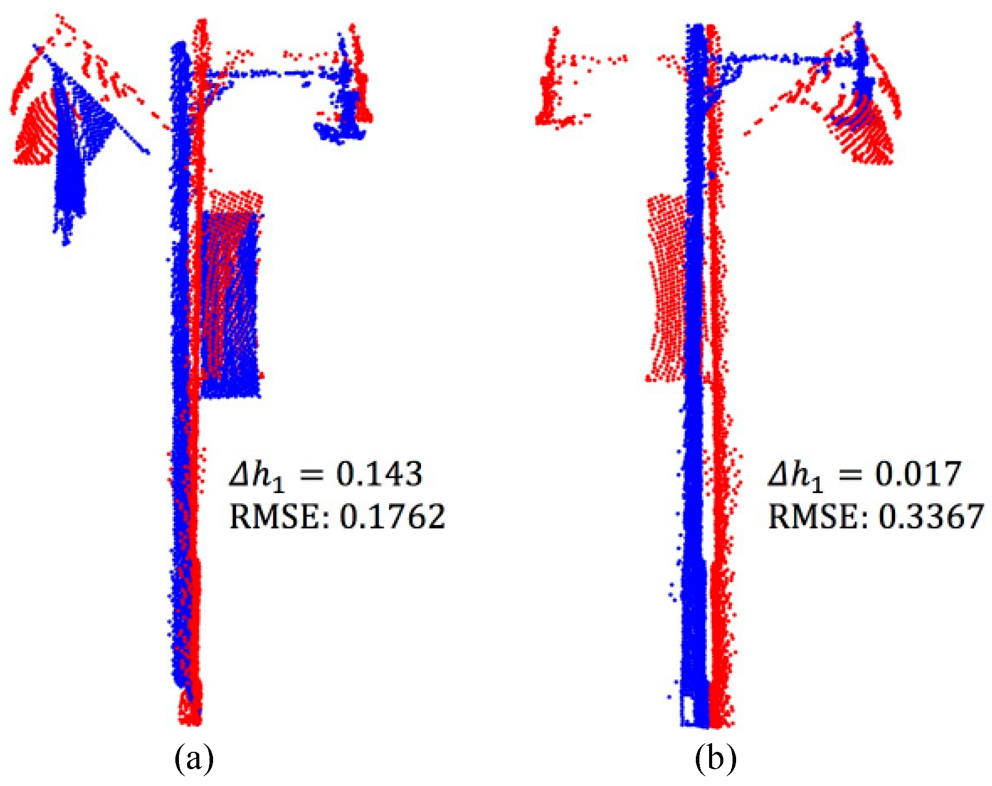
The shape of the street lamps in different scenarios is usually different. The template should be chosen according to the category of street lamps. Figure 18 shows all street lamps with different shapes in the point clouds. The street lamps shown in Figure 18a,c are simple street lamps with a single function, and the other street lamps are complex street lamps with multiple functions. Flags, signs and traffic lights are attached to the simple poles to form complex street lamps. There are two subcategories of street lamp in Data II: Subcategory I (see Figure 18c–g) and Subcategory II (see Figure 18h). In Data II, Subcategory I is the main category of street lamp, and Subcategory II has two. The street lamp shown in Figure 18g is the most complicated one, with flag and signs attached to the pole. Traffic signs and lights are attached to Subcategory II, so the street lamp has lighting and guidance functions, as shown Figure 18h. Street lamps with clear and complex shapes should be preferred as templates. Compared to simple street lamps, complex street lamps should be used as templates since they present more precise registrations, as shown in Figure 19. Figure 19b illustrates the result of registration between a simple street lamp and a complex one as the template. The RMSE is larger than the complex street lamp as template. During the classification phase, choosing simple street lamps as templates increases the possibility of shape matching incorrectness and increases the possibility of pole classification errors.
As shown in Figure 11a and Figure 12a,d, the more similar the 3D shape of pole and template, the smaller the RMSE value. However, the smaller RMSE value is not sufficient evidence to indicate that the pole and the template belong to the same category (see Figure 20). The height difference between pole and template needs to be further compared. As shown in Figure 20a, since the utility pole was similar in height to the template, it was misclassified as a street lamp. The discontinuousness of PLO voxels in the Z-axis direction caused by a small amount of occlusion will not affect PLO extraction. However, the pole was misclassified as a traffic sign because it became shorter, as shown in Figure 20b. In the design of the classification algorithm stage, we assumed that the height of street lamps is between those of the traffic sign and the utility pole. When the heights of utility pole and template are similar and the RMSE is small, an incorrect classification will occur, as shown in Figure 20a. The incomplete pole caused by a small amount of obstacles will not affect pole extraction. However, the pole was misclassified as a traffic sign because it became shorter, as shown in Figure 20b.
During the pole extraction phase, trees with an apparent pole structure will be extracted, as shown in Figure 10. These trees were classified as other objects in the classification step. As shown in Figure 20c,d, in comparison with artificial poles, these trees have relatively large volumes. The RMSEs by registering the trees with the template are greater than that of . For the tree shown in Figure 20d, similar to the template in height, the RMSE is still greater than . In this paper, the method focuses on the extraction and classification of artificial poles, so the extraction and classification accuracy of the trees are not discussed. For future studies, we will focus on the recognition of trees.
The registration result and the height difference between the objects and the template are used for classification. The point on the object forms a point pair with the nearest point on the template to calculate the RMSE. If the size of poles (e.g., traffic signs) is smaller than the template, the poles would match the template segments. Since these PLOs have a pole structure, matching can be performed, and PLOs can be distinguished based on height difference. In future research, the 3D shape matching method can be used according to feature points, which might be more efficient.
4.3. Comparison with Previous Methods
The proposed method can automatically extract and classify most of PLOs, but it is not easy to compare the findings of this study with previous ones since different road conditions and different accuracy sensors will influence the results of recognition. In addition, most previous studies focused on PLOs extraction, while automatic PLOs classification was under-researched. Even so, a comparison was performed by considering the dataset used in their studies. The detection rate and correct detection rate was 77.7% and 81.0% respectively by method of Lehtomäki, et al. [2], respectively. The poles detection rate of the method of Pu, et al. [1] was 86.9% in Enschede data set and 60.8% in the Espoo data set. A completeness, correctness and accuracy rate of 93.6%, 79.5% and 75.1%, respectively, were achieved by Li and Oude Elberink [4] for PLOs detection. The detection rate for the three data sets tested were 83%, 91% and 83% by the method of El-Halawany and Lichti [8], respectively. The detection rate was about 90% by the method of Teo and Chiu [36]. The method of Rodríguez-Cuenca, et al. [24] detected rates in the two datasets at 94.3% and 95.7%. The method of Yan, et al. [50] detection rate achieved over 91% for five types of light poles and towers. The PLO detection method proposed by Guan, et al. [26] achieved a poles detection ratio of 88.9%. The method of Wu, et al. [19] achieved an average overall accuracy of 98.8% for classifying street lamps and traffic signs.
The average completeness, correctness and quality values for PLOs extraction of our method were 91.6%, 97.3% and 89.4%, respectively. Our proposed method achieved an overall accuracy of 92.3% and 91.3% for classifying street lamps and traffic signs and utility poles in two datasets. The method can classify more kinds of PLOs and has high overall accuracy compared with the previous methods. Two different data sets were used in this study, which are very complex and feature overlapped objects.
5. Conclusions
This paper proposed a complete method for PLOs recognition. Point clouds from both town and urban scenes were used to test the proposed method. Firstly, the original data was preprocessed through removing outliers, downsampling and ground filtering. Then, the PLOs were extracted according to the independence analysis and cylindrical or linear feature detection. At last, the PLOs were classified into street lamp, traffic sign, and utility pole by the 3D shape matching method. The method only used , , and coordinates without additional data or training data, and the parameters or thresholds were adjusted according to the structures of different pole-like objects. The PLOs with low point density can also be extracted from point cloud. The correctness was more than 97% in both point clouds. The overall accuracy was 92.3% and 91.3%, respectively. The main advantages of the method are as follows: (1) rapidly extracts poles by spatial and geometric features of the PLO. The potential PLO was extracted at the voxel scale, and then cylindrical and linear feature detection for the potential PLO; (2) classify complex poles based on the method of 3D shape matching. Artificial poles were classified into three categories: Street lamp, traffic sign, and utility pole. The experimental results showed that the proposed method has a high robustness. Our proposed method can effectively extract and classify PLOs, which provides technical support for road maintenance, safety inspection and city modelling using MLS data.
Considering the importance of forest tree species in urban landscape construction and 3D city modeling, it is necessary to focus on automatic extraction and classification of urban trees, which will be covered in our future work.
Author Contributions
Funding acquisition, Y.L. (Yi Lin); Investigation, Z.S. and Z.K.; Methodology, Z.S. and Z.K.; Supervision, Y.L. (Yi Lin); Validation, Z.S., Y.L. (Yi Lin), Y.L. (Yu Liu) and W.C.; Writing–original draft, Z.S.; Writing–review & editing, Y.L. (Yi Lin).
Funding
This work was financially supported in part by the National Natural Science Foundation of China (Grant No. 41471281 and 31670718) and in part by the SRF for ROCS, SEM, China.
Acknowledgments
We are very thankful to the Data II provided by the ISPRS Technical Commission III and the Optech company. The constructive comments and suggestions from three reviewers helped improve the manuscript significantly.
Conflicts of Interest
The authors declare no conflict of interest.
References
- Pu, S.; Rutzinger, M.; Vosselman, G.; Oude Elberink, S. Recognizing basic structures from mobile laser scanning data for road inventory studies. ISPRS J. Photogramm. Remote Sens. 2011, 66, S28–S39. [Google Scholar] [CrossRef]
- Lehtomäki, M.; Jaakkola, A.; Hyyppä, J.; Kukko, A.; Kaartinen, H. Detection of Vertical Pole-Like Objects in a Road Environment Using Vehicle-Based Laser Scanning Data. Remote Sens. 2010, 2, 641–664. [Google Scholar] [CrossRef] [Green Version]
- Jaakkola, A.; Hyyppä, J.; Hyyppä, H.; Kukko, A. Retrieval Algorithms for Road Surface Modelling Using Laser-Based Mobile Mapping. Sensors 2008, 8, 5238–5249. [Google Scholar] [CrossRef] [PubMed] [Green Version]
- Li, D.; Oude Elberink, S. Optimizing detection of road furniture (pole-like object) in Mobile Laser Scanner data. ISPRS Ann. Photogramm. Remote Sens. Spat. Inf. Sci. 2013, 1, 163–168. [Google Scholar] [CrossRef]
- Lehtomäki, M.; Jaakkola, A.; Hyyppä, J.; Kukko, A.; Kaartinen, H. Performance Analysis of a Pole and Tree Trunk Detection Method for Mobile Laser Scanning Data. In Proceedings of the ISPRS Calgary 2011 Workshop, Calgary, AB, Canada, 29–31 August 2011; pp. 197–202. [Google Scholar]
- Aijazi, A.; Checchin, P.; Trassoudaine, L. Segmentation Based Classification of 3D Urban Point Clouds: A Super-Voxel Based Approach with Evaluation. Remote Sens. 2013, 5, 1624–1650. [Google Scholar] [CrossRef] [Green Version]
- Li, Y.; Li, L.; Li, D.; Yang, F.; Liu, Y. A Density-Based Clustering Method for Urban Scene Mobile Laser Scanning Data Segmentation. Remote Sens. 2017, 9, 331. [Google Scholar] [CrossRef]
- El-Halawany, S.I.; Lichti, D.D. Detecting road poles from mobile terrestrial laser scanning data. GISci. Remote Sens. 2013, 50, 704–722. [Google Scholar] [CrossRef]
- Kukko, A.; Kaartinen, H.; Hyyppä, J.; Chen, Y. Multiplatform Mobile Laser Scanning: Usability and Performance. Sensors 2012, 12, 11712–11733. [Google Scholar] [CrossRef] [Green Version]
- Li, L.; Li, Y.; Li, D. A method based on an adaptive radius cylinder model for detecting pole-like objects in mobile laser scanning data. Remote Sens. Lett. 2015, 7, 249–258. [Google Scholar] [CrossRef]
- Zheng, H.; Tan, F.T.; Wang, R.S. Pole-Like Object Extraction from Mobile Lidar Data. Int. Arch. Photogramm. Remote Sens. Spat. Inf. Sci. 2016, 41, 729–734. [Google Scholar] [CrossRef]
- Yadav, M.; Lohani, B.; Singh, A.K.; Husain, A. Identification of pole-like structures from mobile lidar data of complex road environment. Int. J. Remote Sens. 2016, 37, 4748–4777. [Google Scholar] [CrossRef]
- Yadav, M.; Singh, A.K.; Lohani, B. Extraction of road surface from mobile LiDAR data of complex road environment. Int. J. Remote Sens. 2017, 38, 4655–4682. [Google Scholar] [CrossRef]
- Wang, C.; Ji, R.; Wen, C.; Weng, S.; Li, J.; Chen, Y.; Wang, C. Road traffic sign detection and classification from mobile LiDAR point clouds. In Proceedings of the 2nd ISPRS International Conference on Computer Vision in Remote Sensing (CVRS 2015), Xiamen, China, 28–30 April 2015. [Google Scholar]
- Yu, Y.T.; Li, J.; Guan, H.Y.; Wang, C.; Yu, J. Semiautomated Extraction of Street Light Poles From Mobile LiDAR Point-Clouds. IEEE Trans. Geosci. Remote Sens. 2015, 53, 1374–1386. [Google Scholar] [CrossRef]
- Yadav, M.; Husain, A.; Singh, A.K.; Lohani, B. Pole-Shaped Object Detection Using Mobile Lidar Data in Rural Road Environments. Int. Arch. Photogramm. Remote Sens. Spat. Inf. Sci. 2015, 3, 11–16. [Google Scholar] [CrossRef]
- Cabo, C.; Ordoñez, C.; García-Cortés, S.; Martínez, J. An algorithm for automatic detection of pole-like street furniture objects from Mobile Laser Scanner point clouds. ISPRS J. Photogramm. Remote Sens. 2014, 87, 47–56. [Google Scholar] [CrossRef]
- Lim, E.H.; Suter, D. 3D terrestrial LIDAR classifications with super-voxels and multi-scale Conditional Random Fields. Comput. Aided Des. 2009, 41, 701–710. [Google Scholar] [CrossRef]
- Wu, F.; Wen, C.L.; Guo, Y.L.; Wang, J.J.; Yu, Y.T.; Wang, C.; Li, J. Rapid Localization and Extraction of Street Light Poles in Mobile LiDAR Point Clouds: A Supervoxel-Based Approach. IEEE Trans. Intell. Transp. Syst. 2017, 18, 292–305. [Google Scholar] [CrossRef]
- Rabbani, T.; Van Den Heuvel, F. Efficient hough transform for automatic detection of cylinders in point clouds. In Proceedings of the Workshop “Laser Scanning 2005”, Enschede, The Netherlands, 12–14 September 2005; pp. 60–65. [Google Scholar]
- Lam, J.; Kusevic, K.; Mrstik, P.; Harrap, R.; Greenspan, M. Urban Scene Extraction from Mobile Ground Based LiDAR Data. In Proceedings of the 5th International Symposium on 3D Data Processing, Visualization and Transmission, Paris, France, 17–20 May 2010; pp. 1–8. [Google Scholar]
- Hu, Y.; Li, X.; Xie, J.; Guo, L. A Novel Approach to Extracting Street Lamps from Vehicle-borne Laser Data. In Proceedings of the 2011 19th International Conference on Geoinformatics, Shanghai, China, 24–26 June 2011; pp. 1–6. [Google Scholar]
- Yan, L.; Li, Z.; Liu, H.; Tan, J.; Zhao, S.; Chen, C. Detection and classification of pole-like road objects from mobile LiDAR data in motorway environment. Opt. Laser Technol. 2017, 97, 272–283. [Google Scholar] [CrossRef]
- Rodríguez-Cuenca, B.; García-Cortés, S.; Ordóñez, C.; Alonso, M. Automatic Detection and Classification of Pole-Like Objects in Urban Point Cloud Data Using an Anomaly Detection Algorithm. Remote Sens. 2015, 7, 12680–12703. [Google Scholar] [CrossRef] [Green Version]
- Reed, I.S.; Yu, X. Adaptive multiple-band CFAR detection of an optical pattern with unknown spectral distribution. IEEE Trans. Acoust. Speech Signal Process. 1990, 38, 1760–1770. [Google Scholar] [CrossRef]
- Guan, H.; Yu, Y.; Li, J.; Liu, P. Pole-Like Road Object Detection in Mobile LiDAR Data via Supervoxel and Bag-of-Contextual-Visual-Words Representation. IEEE Geosci. Remote Sens. Lett. 2016, 13, 520–524. [Google Scholar] [CrossRef]
- Zheng, H.; Wang, R.S.; Xu, S. Recognizing Street Lighting Poles From Mobile LiDAR Data. IEEE Trans. Geosci. Remote Sens. 2017, 55, 407–420. [Google Scholar] [CrossRef]
- Hosoi, F.; Omasa, K. Voxel-Based 3-D Modeling of Individual Trees for Estimating Leaf Area Density Using High-Resolution Portable Scanning Lidar. IEEE Trans. Geosci. Remote Sens. 2006, 44, 3610–3618. [Google Scholar] [CrossRef]
- Wu, B.; Yu, B.; Yue, W.; Shu, S.; Tan, W.; Hu, C.; Huang, Y.; Wu, J.; Liu, H. A Voxel-Based Method for Automated Identification and Morphological Parameters Estimation of Individual Street Trees from Mobile Laser Scanning Data. Remote Sens. 2013, 5, 584–611. [Google Scholar] [CrossRef] [Green Version]
- Wang, J.; Lindenbergh, R.; Menenti, M. SigVox—A 3D feature matching algorithm for automatic street object recognition in mobile laser scanning point clouds. ISPRS J. Photogramm. Remote Sens. 2017, 128, 111–129. [Google Scholar] [CrossRef]
- Wang, Y.; Feng, H.-Y. Effects of scanning orientation on outlier formation in 3D laser scanning of reflective surfaces. Opt. Lasers Eng. 2016, 81, 35–45. [Google Scholar] [CrossRef]
- Sotoodeh, S. Outlier detection in laser scanner point clouds. Int. Arch. Photogramm. Remote Sens. Spat. Inf. Sci. 2006, 36, 297–302. [Google Scholar]
- Herrero-Huerta, M.; Lindenbergh, R.; Rodriguez-Gonzalvez, P. Automatic tree parameter extraction by a Mobile LiDAR System in an urban context. PLoS One 2018, 13, e0196004. [Google Scholar] [CrossRef] [PubMed]
- Rusu, R.B.; Marton, Z.C.; Blodow, N.; Dolha, M.; Beetz, M. Towards 3D Point cloud based object maps for household environments. Robot. Autom. Syst. 2008, 56, 927–941. [Google Scholar] [CrossRef]
- Hackel, T.; Wegner, J.D.; Schindler, K. Fast Semantic Segmentation of 3d Point Clouds with Strongly Varying Density. In Proceedings of the 2016 ISPRS Congress, Prague, Czech Republic, 12–19 July 2016. [Google Scholar] [CrossRef]
- Teo, T.A.; Chiu, C.M. Pole-Like Road Object Detection From Mobile Lidar System Using a Coarse-to-Fine Approach. IEEE J. Sel. Top. Appl. Earth Obs. Remote Sens. 2015, 8, 4805–4818. [Google Scholar] [CrossRef]
- Luo, H.; Wang, C.; Wang, H.Y.; Chen, Z.Y.; Zai, D.W.; Zhang, S.X.; Li, J. Exploiting Location Information to Detect Light Pole in Mobile Lidar Point Clouds. Int. Geosci. Remote Sens. 2016. [Google Scholar] [CrossRef]
- Zhang, K.Q.; Chen, S.C.; Whitman, D.; Shyu, M.L.; Yan, J.H.; Zhang, C.C. A progressive morphological filter for removing nonground measurements from airborne LIDAR data. IEEE Trans. Geosci. Remote Sens. 2003, 41, 872–882. [Google Scholar] [CrossRef] [Green Version]
- Vosselman, G. Slope based filtering of laser altimetry data. Int. Arch. Photogramm. Remote Sens. Spat. Inf. Sci. 2000, 33, 935–942. [Google Scholar]
- Zhang, W.M.; Qi, J.B.; Wan, P.; Wang, H.T.; Xie, D.H.; Wang, X.Y.; Yan, G.J. An Easy-to-Use Airborne LiDAR Data Filtering Method Based on Cloth Simulation. Remote Sens. 2016, 8, 501. [Google Scholar] [CrossRef]
- Fischler, M.A.; Bolles, R.C. Random Sample Consensus—A Paradigm for Model-Fitting with Applications to Image-Analysis and Automated Cartography. Commun. ACM 1981, 24, 381–395. [Google Scholar] [CrossRef]
- Kang, Z.Z.; Zhang, L.Q.; Wang, B.Q.; Li, Z.; Jia, F.M. An Optimized BaySAC Algorithm for Efficient Fitting of Primitives in Point Clouds. IEEE Geosci. Remote Sens. Lett. 2014, 11, 1096–1100. [Google Scholar] [CrossRef]
- Kang, Z.; Zhong, R.; Wu, A.; Shi, Z.; Luo, Z. An Efficient Planar Feature Fitting Method Using Point Cloud Simplification and Threshold-Independent BaySAC. IEEE Geosci. Remote Sens. Lett. 2016, 13, 1842–1846. [Google Scholar] [CrossRef]
- Gross, H.; Thoennessen, U. Extraction of Lines From Laser Point Clouds. Int. Arch. Photogramm. Remote Sens. Spat. Inf. Sci. 2006, 36, 86–91. [Google Scholar]
- Yokoyama, H.; Date, H.; Kanai, S.; Takeda, H. Pole-Like Objects Recognition from Mobile Laser Scanning Data Using Smoothing and Principal Component Analysis. Int. Arch. Photogramm. Remote Sens. Spat. Inf. Sci. 2011, 38, 115–120. [Google Scholar] [CrossRef]
- Qin, X.; Wu, G.; Ye, X.; Huang, L.; Lei, J. A Novel Method to Reconstruct Overhead High-Voltage Power Lines Using Cable Inspection Robot LiDAR Data. Remote Sens. 2017, 9, 753. [Google Scholar] [CrossRef]
- Lin, Y.; Hyyppa, J.; Jaakkola, A. Mini-UAV-Borne LIDAR for Fine-Scale Mapping. IEEE Geosci. Remote Sens. Lett. 2011, 8, 426–430. [Google Scholar] [CrossRef]
- Holz, D.; Ichim, A.E.; Tombari, F.; Rusu, R.B.; Behnke, S. Registration with the Point Cloud Library a Modular Framework for Aligning in 3-D. IEEE Robot. Autom. Mag. 2015, 22, 110–124. [Google Scholar] [CrossRef]
- Besl, P.J.; McKay, N.D. A Method for Registration of 3-D Shapes. IEEE Trans. Pattern Anal. Mach. Intell. 1992, 14, 239–256. [Google Scholar] [CrossRef]
- Yan, W.Y.; Morsy, S.; Shaker, A.; Tulloch, M. Automatic extraction of highway light poles and towers from mobile LiDAR data. Opt. Laser Technol. 2016, 77, 162–168. [Google Scholar] [CrossRef]
Figure 1.
Flow chart of pole-like object (PLO) recognition.

Figure 2.
Data I (town scene). (a) Original point cloud; (b) Rough ground classification.

Figure 3.
Data II (urban scene). (a) Original point cloud; (b) Rough ground classification.

Figure 4.
Voxel used in this study. (a) Coordinate system of voxel; (b) 8-neighbors in the same layer; (c) 3-neighbors in the vertical direction.
Figure 4.
Voxel used in this study. (a) Coordinate system of voxel; (b) 8-neighbors in the same layer; (c) 3-neighbors in the vertical direction.

Figure 5.
Point cloud voxelization. (a) Original dataset; (b) Regular voxels.

Figure 6.
Space structure of PLO voxels. (a) PLO voxels; (b) Neighborhood voxels; (c) Top view of (b); (d) The side view of (b).
Figure 6.
Space structure of PLO voxels. (a) PLO voxels; (b) Neighborhood voxels; (c) Top view of (b); (d) The side view of (b).

Figure 7.
Cylindrical feature detection. (a) Street lamp and point set with independence; (b) Fitting cylinder; (c) Interior points and exterior points.
Figure 7.
Cylindrical feature detection. (a) Street lamp and point set with independence; (b) Fitting cylinder; (c) Interior points and exterior points.

Figure 8.
Templates. (a) Template I; (b) Template II; (c) Template III.

Figure 9.
Results of PLOs extraction in Data I. (a) Non-ground points colored in cyan and PLOs colored in black; (b) view 1; (c) view 2.
Figure 9.
Results of PLOs extraction in Data I. (a) Non-ground points colored in cyan and PLOs colored in black; (b) view 1; (c) view 2.

Figure 10.
Results of PLOs extraction in Data II. (a) Non-ground points colored in cyan and PLOs colored in black; (b) view 1; (c) view 2.
Figure 10.
Results of PLOs extraction in Data II. (a) Non-ground points colored in cyan and PLOs colored in black; (b) view 1; (c) view 2.

Figure 11.
Illustration of the results for three-dimensional (3D) shape matching of poles in Data I (the template was illustrated in Figure 8). (a–d) are the classified poles of a street lamp, a traffic sign, a street lamp and a utility pole, respectively.
Figure 11.
Illustration of the results for three-dimensional (3D) shape matching of poles in Data I (the template was illustrated in Figure 8). (a–d) are the classified poles of a street lamp, a traffic sign, a street lamp and a utility pole, respectively.

Figure 12.
Illustration of the results for 3D shape matching results of poles in Data II (the templates were illustrated in Figure 8). (a,b) are the classified poles of a street lamp and a traffic sign, respectively; (c) The pole cannot be classified as a street lamp based on Template II; (d) The pole (see (c)) is classified as a street light after being matched with Template III.

Figure 13.
Results of PLO recognition in Data I. Different colors represent the different class.

Figure 14.
Undetected utility pole that is surrounded by the canopy.

Figure 15.
Results of PLO recognition in Data II. Different colors represent different classes.

Figure 16.
Undetected street lamp due to high crown and low vegetation.

Figure 17.
Wrongly detected building pillar as pole.

Figure 18.
Differently shaped street lamps. (a,b) belong to Data I; (c–h) belong to Data II.

Figure 19.
Registration differences between the same pole and different templates. (a) Complex street lamp as template; (b) Simple street lamp as template.
Figure 19.
Registration differences between the same pole and different templates. (a) Complex street lamp as template; (b) Simple street lamp as template.

Figure 20.
(a) Falsely classified utility pole as a street lamp; (b) Part of street lamp was misclassified as a traffic sign; (c) The big tree was classified as other object after matching the template; (d) The small tree was also classified as other object.
Figure 20.
(a) Falsely classified utility pole as a street lamp; (b) Part of street lamp was misclassified as a traffic sign; (c) The big tree was classified as other object after matching the template; (d) The small tree was also classified as other object.


Table 1.
Mobile Laser Scanning (MLS) Point cloud information.
| Data | Original Points | Removed Points | Non-Ground Points | |
|---|---|---|---|---|
| Data I | 8,139,726 | 733 | 1,703,153 (20.9%) | 2,202,120 (27%) |
| Data II | 35,527,813 | 4183 | 11,112,865 (31.3%) | 7,795,873 (21.9%) |
Table 2.
Features used in the process of classification.
| Classification Features | Description | |
|---|---|---|
| Shape | The street lamp with high point density and clear shape in the raw point cloud. | |
| The unclassified poles are used as input data for the classification process. | ||
| RMSE | RMSE is used to judge whether the 3D shape matching is successful. If RMSE is greater than , will be classified as others. | |
| If the RMSE value is between and , falls in the utility pole category. If the RMSE is less than or equal to , the category of needs to be further judged based on the height feature. | ||
| Height | If is less than or equal to , belongs to the category street lamp. | |
| If is greater than , then can be classified to be category traffic signal, otherwise it is a utility pole. and denote different levels of height difference between and , . | ||
Table 3.
Parameters used for classification pole-like objects (PLOs).
| Data | |||||
|---|---|---|---|---|---|
| Data I | 0.80 | 0.15 | 1.5 | 3.00 | 3.6 |
| Data II | 0.80 | 0.20 | 1.0 | 1.50 | 3.6 |
Table 4.
PLO extraction quality.
| Data | TP | FP | FN | Completeness | Correctness | Quality |
|---|---|---|---|---|---|---|
| Data I | 38 | 1 | 3 | 92.7% | 97.4% | 90.5% |
| Data II | 67 | 2 | 7 | 90.5% | 97.1% | 88.2% |
Table 5.
Quality of classification results of PLOs.
| Data | Street Lamp | Utility Pole | Traffic Sign | Others | Precision (%) | |
|---|---|---|---|---|---|---|
| Data I | Street lamp | 22 | 2 | 0 | 0 | 91.7 |
| Utility pole | 0 | 10 | 0 | 0 | 100.0 | |
| Traffic sign | 0 | 0 | 4 | 1 | 80.0 | |
| OA: 36/39 = 92.3% | ||||||
| Data II | Street lamp | 35 | 2 | 1 | 0 | 92.1 |
| Utility pole | 1 | 1 | 0 | 0 | 50.0 | |
| Traffic sign | 0 | 0 | 27 | 2 | 93.1 | |
| OA: 63/69 = 91.3% | ||||||
Table 6.
Processing time cost by each stage of our method (seconds).
| Data | Preprocessing | 2nd Voxelization | Independence Analysis | Features Detection | PLOs Classification | Total Time |
|---|---|---|---|---|---|---|
| Data I | 126.3 | 0.4 | 1.8 | 41.6 | 139.5 | 309.6 |
| Data II | 381.4 | 1.1 | 15.7 | 237.5 | 813.6 | 1449.3 |
Table 7.
The different characteristics between Data I and Data II.
| Data | Objects | Poles | Topography | |
|---|---|---|---|---|
| Diameter (m) | Height (m) | Maximum Gradient | ||
| Data I | Houses, poles, trees, lawn, people, vehicles | 0.23, 0.27,0.13 | 6.32, 7.42, 2.70 | 2.2% |
| Data II | Buildings, poles, trees, people, vehicles | 0.21, 0.35, 0.08 | 5.75, 11.83, 3.07 | 3.0% |
© 2018 by the authors. Licensee MDPI, Basel, Switzerland. This article is an open access article distributed under the terms and conditions of the Creative Commons Attribution (CC BY) license (http://creativecommons.org/licenses/by/4.0/).
Share and Cite
MDPI and ACS Style
Shi, Z.; Kang, Z.; Lin, Y.; Liu, Y.; Chen, W. Automatic Recognition of Pole-Like Objects from Mobile Laser Scanning Point Clouds. Remote Sens. 2018, 10, 1891. https://0-doi-org.brum.beds.ac.uk/10.3390/rs10121891
AMA Style
Shi Z, Kang Z, Lin Y, Liu Y, Chen W. Automatic Recognition of Pole-Like Objects from Mobile Laser Scanning Point Clouds. Remote Sensing. 2018; 10(12):1891. https://0-doi-org.brum.beds.ac.uk/10.3390/rs10121891
Chicago/Turabian StyleShi, Zhenwei, Zhizhong Kang, Yi Lin, Yu Liu, and Wei Chen. 2018. "Automatic Recognition of Pole-Like Objects from Mobile Laser Scanning Point Clouds" Remote Sensing 10, no. 12: 1891. https://0-doi-org.brum.beds.ac.uk/10.3390/rs10121891
Note that from the first issue of 2016, this journal uses article numbers instead of page numbers. See further details here.