A Comparative Assessment of Different Modeling Algorithms for Estimating Leaf Nitrogen Content in Winter Wheat Using Multispectral Images from an Unmanned Aerial Vehicle

Abstract

Unmanned aerial vehicle (UAV)-based remote sensing (RS) possesses the significant advantage of being able to efficiently collect images for precision agricultural applications. Although numerous methods have been proposed to monitor crop nitrogen (N) status in recent decades, just how to utilize an appropriate modeling algorithm to estimate crop leaf N content (LNC) remains poorly understood, especially based on UAV multispectral imagery. A comparative assessment of different modeling algorithms (i.e., simple and non-parametric modeling algorithms alongside the physical model retrieval method) for winter wheat LNC estimation is presented in this study. Experiments were conducted over two consecutive years and involved different winter wheat varieties, N rates, and planting densities. A five-band multispectral camera (i.e., 490 nm, 550 nm, 671 nm, 700 nm, and 800 nm) was mounted on a UAV to acquire canopy images across five critical growth stages. The results of this study showed that the best-performing vegetation index (VI) was the modified renormalized difference VI (RDVI), which had a determination coefficient (R²) of 0.73 and a root mean square error (RMSE) of 0.38. This method was also characterized by a high processing speed (0.03 s) for model calibration and validation. Among the 13 non-parametric modeling algorithms evaluated here, the random forest (RF) approach performed best, characterized by R² and RMSE values of 0.79 and 0.33, respectively. This method also had the advantage of full optical spectrum utilization and enabled flexible, non-linear fitting with a fast processing speed (2.3 s). Compared to the other two methods assessed here, the use of a look up table (LUT)-based radiative transfer model (RTM) remained challenging with regard to LNC estimation because of low prediction accuracy (i.e., an R² value of 0.62 and an RMSE value of 0.46) and slow processing speed. The RF approach is a fast and accurate technique for N estimation based on UAV multispectral imagery.

1. Introduction

Nitrogen (N) is one of the most important nutrients required for plant growth and is therefore critical for crop production. A deficiency in N significantly reduces crop photosynthetic yields while the excessive use of fertilizers for this element leads to both resource waste and environmental pollution [1,2]. Furthermore, leaf N content (LNC) at early growth stages (e.g., jointing and booting) is a good indicator for N fertilizer application [3], and LNC at late growth stages (e.g., after heading) is highly related to the final grain quality [4]. Quantification of LNC is therefore a prerequisite for the production of high-yield and good-quality crops while causing minimal environmental impact.

Remote sensing (RS) has become an attractive technique in precision agricultural assessment as it can be used to monitor crop growth status rapidly and nondestructively. The main RS platforms currently in use include satellite, manned airborne, and ground-based approaches, which can all be equipped with various kinds of sensors. Although satellite images can be used to monitor N status across large areas [5,6], they cannot provide sufficient accuracy because of their low spatio-temporal resolution. Even though manned airborne platforms are able to capture images at high spatio-temporal resolution, this approach is limited by both high operational complexity and cost [7].

In contrast, ground-based RS platforms are able to attain high N status estimation monitoring accuracy [8,9], but this approach remains inefficient when used over large areas, while unmanned aerial vehicle (UAV)-based RS platforms provide a low-cost alternative for collecting RS data at high spatio-temporal resolution [10,11]. This platform has been widely applied in precision agriculture and has been utilized for LAI [12] as well as biomass estimations [10,13], but few studies to date have discussed N status detection using this approach [14,15]. It therefore remains an open question whether, or not, UAV images can be used to monitor N status.

A range of methods have so far been proposed that use spectral data to model N content, including statistical and chemometric algorithms alongside physical models. The statistical method has been used most commonly to monitor N content based on optical measurements from different platforms [8,16]. Empirical relationships between LNC and canopy optical properties have also been calibrated using experimental datasets, an approach that has proven to be both efficient and accurate [8,9,17]. It is also the case, however, that retrieval algorithms based on vegetation indices (VIs) tend to exhibit poor model portability because they are easily influenced by band configuration, index formulation, and fitting function [18]. Besides, most VIs are easily saturated at high N content levels [8,19].

An additional set of techniques that have been commonly applied to identify variables for N modeling comprise non-parametric algorithms, including partial least square regression (PLSR), artificial neural networks (ANNs), random forest (RF), and support vector machines (SVMs) [3,20,21]. These approaches make full use of all spectral data and avoid multicollinearity that is inherent to multiple linear regressions [20]. As these methods have also been shown to be very efficient for processing nonlinear data, it is likely that they are also able to deal with high-dimensional data [21] although performance remains an issue [22,23]. In the earlier study, Verrelst et al. [23] investigated the efficiency of four machine learning regression algorithms at estimating leaf chlorophyll content (LCC), LAI, and fractional vegetation cover (FVC), specifically neural networks (NN), support vector regression (SVR), kernel ridge regression (KRR), and Gaussian processes regression (GPR). As the results of this study showed that the latter was more efficient compared to the other three [23], it will also be worthwhile to investigate the performance of different non-parametric algorithms for LNC estimation.

It remains challenging to quantify LNC differences based on small-plot experiments using several cultivars as well as N application levels and planting densities. As differences in N content under experimental conditions are generally limited, established models might be unstable in practical applications. It is also the case that a significant component of variations in canopy optical properties are also due to changes in sun zenith angles, canopy structures, and background. As these differences significantly affect the relationships between spectral parameters and N content, a model based on physical parameters should enable us to clearly explain these potentially confounding factors. Although a PROSAIL radiative transfer model (RTM) [24] used in combination with hyperspectral reflectance has been shown to provide an effective method for estimating crop LAI [25,26] and LCC [27], it remains unclear how this approach can be utilized to offer enough LNC estimation accuracy with UAV multispectral imagery.

The different modeling algorithms discussed above were studied here using a range of species and sites. One key aim of this research was to comprehensively compare these approaches and determine the optimal retrieval method for a particular objective, especially when using UAV images. A range of questions remains to be addressed, including which VI is optimal for wheat LNC estimation? Which non-parametric algorithm provides the best estimates? How well do physical models perform for LNC retrieval when based on UAV multispectral images? Additionally, which is the best approach when all three modeling algorithms are compared in terms of processing efficiency, model simplification, and estimation accuracy? The objective of this study was therefore to evaluate the performance of these three different retrieval methods for winter wheat LNC estimation using UAV multispectral imagery.

2. Materials and Methods

2.1. Experimental Design

Three field experiments were conducted over two growing seasons (2013–2014 and 2014–2015) in Rugao City (120°45′E, 32°16′N) within Jiangsu Province in eastern China. The predominant soil type is loam and the soil organic matter was 18.9–24.6 g/kg, available N was 140.56–150.41 mg/kg, total nitrogen was 1.87–2.07 g/kg, available phosphorus was 50.12–57.84 mg/kg, and available potassium was 90.32–96.76 mg/kg. These experiments involved different N rates, planting densities, and wheat cultivars, and comprised a randomized complete block design with three replicates, thus there were 36, 30, and 36 treatments for Exp. 1, Exp. 2, and Exp. 3, respectively. A mixture of 120 kg/ha P₂O₅ and 120 kg/ha K₂O was applied to all treatments prior to seeding. Crop management followed local standard practices for wheat production; additional details regarding these three experiments are provided in

Table 1. Details of the three field experiments.

Experiment	Year	Cultivar	N Rate (kg/ha)	Planting Density (plants/ha)	Sampling Date	Growth Stage	N
Exp. 1	2013–2014	Yangmai 18 Shengxuan 6	0, 100, 300	1.5 × 106 3.0 × 106	14 March 9/15/23 April 6 May	Jointing, Booting, Heading, Anthesis, Filling	159
Exp. 2	2013–2014	Xumai 30 Ningmai 13	0, 75, 150, 225, 300	2.4 × 106	14 March 9/15/23 April 6 May	Jointing, Booting, Heading, Anthesis, Filling	135
Exp. 3	2014–2015	Yangmai 18 Shengxuan 6	0, 100, 300	1.5 × 106 2.4 × 106	26 March 8/17/25 April 6 May	Jointing, Booting, Heading, Anthesis, Filling	164

.

2.2. Data Collection

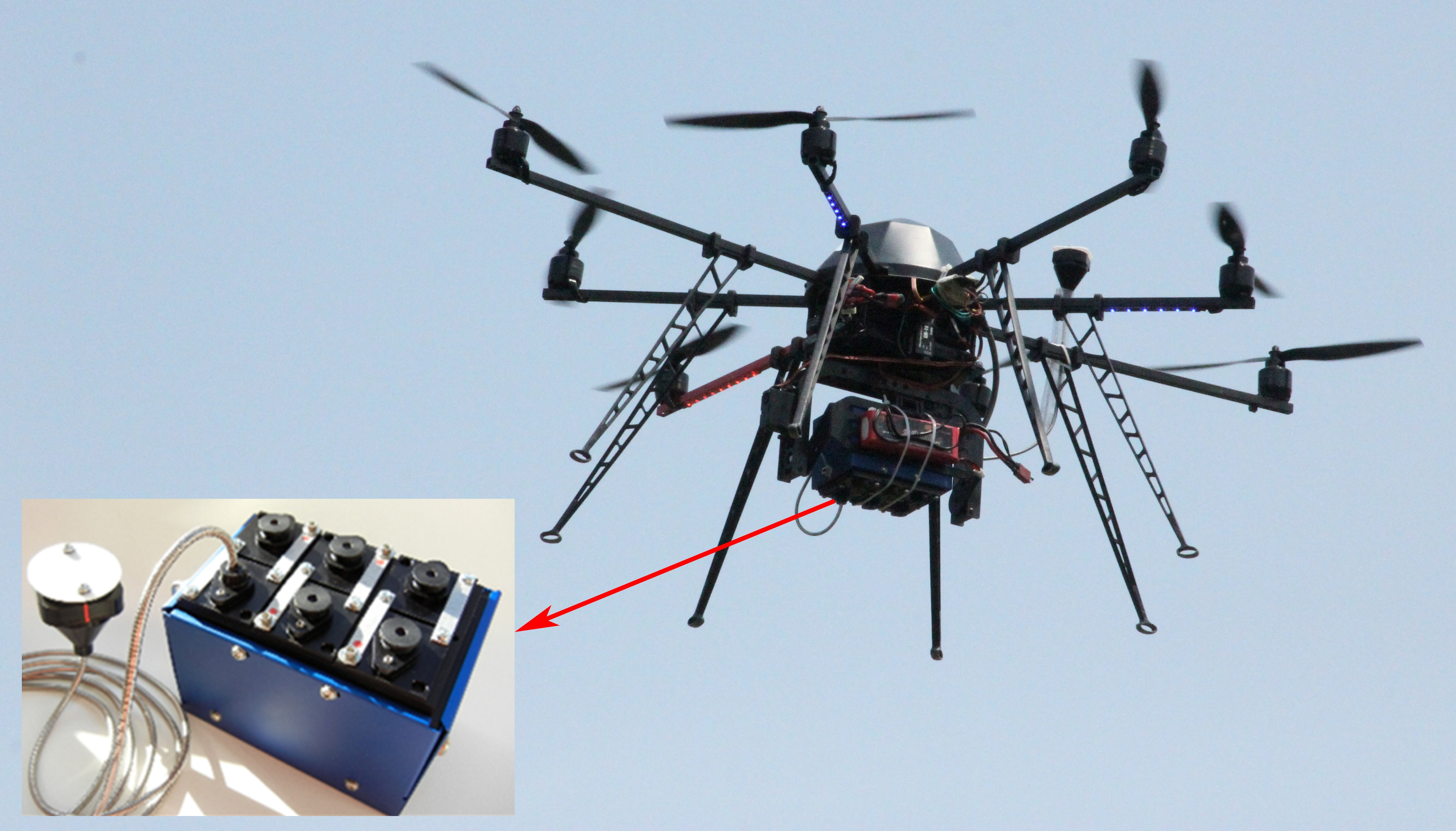
2.2.1. UAV System and Image Acquisition

An eight-rotor MK-Oktokopter UAV (Mikrokopter Inc., Moormerland, Germany) was used to carry a six-channel multispectral Tetracam mini-MCA6 camera (Tetracam Inc., Chatsworth, CA, USA) to collect images in this study (Figure 1). The specific parameters of this UAV and camera are shown in

Table 2. Specifications of UAV and Mini-MCA multispectral camera.

UAV		Camera
Weight (g)	2050	Weight (g)	700
Battery weight (g)	520	Geometric resolution (pixel)	1280 × 1024
Maximum payload (g)	2500	Radiometric resolution (bit)	10
Flight duration (min)	8–41	Speed (frame/s)	1.3
Radius (m)	1000	Focal length (mm)	9.6

. This multispectral camera was equipped with five spectral channels (i.e., 490 nm, 550 nm, 671 nm, 700 nm, and 800 nm) with a 10 nm bandwidth, and had an incident light sensor (ILS). All UAV campaigns were undertaken in stable ambient light conditions (between 11:00 and 13:30) at five critical growth stages (Table 1). The UAV was flown at a height of 150 m, and images were collected with spatial resolution of 8.125 cm. After each flight, only one image with high quality was selected for image analysis due to the small study area (50 m × 35 m).

2.2.2. Ground Sampling

A total of 30 wheat plant samples were randomly collected from each plot subsequent to each UAV campaign in order to determine LNC values (%). All the green leaves from each sample were separated from stems, oven-dried at 80 °C to a constant weight, and then weighed. Dried leaf samples were ground to pass through a 1 mm screen and stored in plastic bags for subsequent chemical analysis. Total leaf N concentration was determined using the micro-Kjeldahl method. Leaf chlorophyll content (Cab) was measured using a soil and plant analyzer development (SPAD) 502 (Minolta Camera Co., Osaka, Japan) with sub-samples (five plants) randomly selected and the first, second, and third fully expanded leaves chosen from three layers encompassing the base, middle, and top parts of wheat leaves. Averaged SPAD readings were taken as sample values in each case. Absolute leaf chlorophyll content (LCC) was then obtained using an equation that expresses the relationship between SPAD readings and LCC values [28].

2.3. Image Processing

The pre-processing UAV image workflows used in this analysis followed those proposed by [12,29], and included noise reduction, veginetting, and lens distortion correction as well as band registration and radiometric calibration. Thirty ground control points (GCPs) were evenly distributed in the experimental area, and the geographic coordinates were determined by X900 GNSS (Huace Inc., Beijing, China). The GCPs were used for band registration and georeferencecing processed in the ENVI/IDL environment (Exelis Visual Information Solutions, Boulder, CO, USA). After that, radiometric calibration was conducted by the empirical line method [30] with four standard calibration canvas with different reflectance values (3%, 22%, 48%, and 82%). Reflectance was then extracted from each radiometrically corrected image using a region of interest (ROI) from each plot.

2.4. Retrieval Techniques

2.4.1. Parametric Modeling Algorithms

The parametric modeling algorithm used in this analysis was based on VI calculated with reflectance from UAV multispectral images. Thus, 19 kinds of VI formulations, including two-band, three-band, and four-band indices, encompassing all possible combinations were used to develop correlations versus wheat LNC (

Table 3. Commonly used vegetation indices.

Index	Formula	Reference
Two-band
Ratio VI (RVI)	Rλ1/Rλ2	[31]
Difference VI (DVI)	Rλ1 − Rλ2	[31]
NDVI	(Rλ1 − Rλ2)/(Rλ1 + Rλ2)	[32]
Renormalized difference VI (RDVI)	(Rλ1 − Rλ2)/(Rλ1 + Rλ2)0.5	[33]
Soil adjusted VI (SAVI)	1.5(Rλ1 − Rλ2)/(Rλ1 + Rλ2 + 0.5)	[34]
Optimized soil adjusted VI (OSAVI)	(1 + 0.16)(Rλ1 − Rλ2)/(Rλ1 + Rλ2 + 0.16)	[35]
Optimized VI (VIopt)	(1 + 0.45)(Rλ12 + 1)/(Rλ2 + 0.45)	[36]
Modified sample ratio (MSR)	((Rλ1/Rλ2) − 1)/(SQRT((Rλ1/Rλ2) + 1))	[37]
Three-band
Enhanced VI (EVI)	2.5(Rλ1 − Rλ2)/(Rλ1 + 6Rλ2 − 7.5Rλ3 + 1)	[38]
Modified normalized difference (mND)	(Rλ1 − Rλ2)/(Rλ1 + Rλ2 − 2Rλ3)	[39]
Modified sample ratio (mSR)	(Rλ1 − Rλ2)/(Rλ3 − Rλ2)	[39]
Modified chlorophyll absorption in RI (MCARI)	(Rλ1 − Rλ2 − 0.2(Rλ1 − Rλ3))(Rλ1/Rλ2)	[40]
Transformed chlorophyll absorption in RI (TCARI)	3((Rλ1 − Rλ2) − 0.2(Rλ1 − Rλ3)(Rλ1/Rλ2))	[41]
Three-band index 1 (TBI1)	(Rλ1 − Rλ2 − Rλ3)/(Rλ1 + Rλ2 + Rλ3)	[42]
Three-band index 2 (TBI2)	(Rλ1 − Rλ2 + 2Rλ3)/(Rλ1 + Rλ2 − 2Rλ3)	[17]
Four-band
Vogelmann index (VOG)	(Rλ1 − Rλ2)/(Rλ3 + Rλ4)	[43]
MERIS terrestrial chlorophyll index (MTCI)	(Rλ1 − Rλ2)/(Rλ3 − Rλ4)	[44]
TCARI/OSAVI	TCARI/OSAVI	[41]
MCARI/OSAVI	MCARI/OSAVI	[40]

R_λ1, R_λ2, R_λ3, and R_λ4 denote the reflectance of spectral bands randomly selected from 490 nm, 550 nm, 671 nm, 700 nm, and 800 nm.

). Linear regression between LNC and all VIs was utilized to eliminate the impact of functions as opposed to band selection and index formulation.

2.4.2. Non-Parametric Modeling Algorithms

The SimpleR toolbox [45] was used in this study to implement 13 non-parametric modeling algorithms and to develop models. A comprehensive description of these algorithms was presented in [46]. These non-parametric approaches can be further subdivided into linear and non-linear regressions; of these, three fall into the former category-least-squares linear regression (LSLR), principal component regression (PCR), and partial least-squares regression (PLSR)-while 10 fall into the latter-artificial neutral networks (ANN), decision trees (DT), regression trees (RT), bagging trees (BaT), and boosting trees (BoT) as well as random forest (RF), relevance vector machine (RVM), kernel ridge (KRR), and Gaussian processes regressions (GPR) alongside variational heteroscedastic GPR (VH-GPR) and extreme learning machines (ELM).

2.4.3. Physical Based Modeling

The widely used PROSAIL radiative transfer model comprises a combination of the SAIL canopy reflectance and PROSPECT leaf optical properties models. The combined approach was utilized here to retrieve canopy parameter data and was generated via both the latter two methods, PROSPECT-5 and 4SAIL. A look-up-table (LUT) was then applied; these efficient inversion algorithms are commonly used for agronomic parameter retrieval [46,47]. The imposed boundaries and distributions of PROSAIL input variables used in this study are summarized in

Table 4. PROSAIL model input parameters.

Parameters	Units	Range	Distribution
Leaf: PROSPECT-5
Leaf structure index (N)	Unitless	1.2–1.8	Gaussian
Leaf chlorophyll content (LCC)	[μg/cm2]	25–75	Gaussian
Leaf dry matter content (Cm)	[g/cm2]	0.013
Leaf water content (Cw)	[cm]	0.018
Canopy: 4SAIL
Leaf area index (LAI)	[m2/m2]	0–7	Gaussian
Soil scaling factor (αsoil)	Unitless	0.3
Average leaf angle (ALA)	[°]	60
Hotspot parameter (HotS)	[m/m]	0.2
Diffuse incoming solar radiation (skyl)	[%]	10
Sun zenith angle (θs)	[°]	25
View zenith angle (θv)	[°]	0
Sun-sensor azimuth angle (Φ)	[°]	0

; these values were obtained from field measurements and other studies that have utilized the same crops [47,48]. Thus, uniform distributions of LCC and normally distributed LAI were sampled 100 times, uniform carotenoid distributions were sampled 50 times, and all other variables were held constant. A resultant LUT dataset comprising 500,000 parameter combinations was chosen for this analysis; a total of 22 cost functions, including the insertion of up to 50% Gaussian noise into simulated data and multiple best solutions, were considered to optimize the LUT inversion strategy to address radiative transfer model issues [49]. After LCC was retrieved from the PROSAIL model, LNC was indirectly obtained on the empirically linear relationship between LCC and LNC.

2.5. Model Calibration and Validation

Table 5. Calibration and validation of the models on different methods.

Method	Calibration	Validation
Parametric	10-fold cross validation, nine sub-datasets used for calibration (training), the rest for validation (test), repeated 10 times
Non-parametric
Physical-based model	LCC retrieved from PROSAIL, LNC obtained through the empirically linear model between LCC and LNC with measured data	All retrieved LNC values compared with measured LNC values

lists the calibration and validation of models on different methods. Data collected from all experiments were pooled to examine the relationship between VIs and LNC with linear regression, and then the optimal bands’ configurations were determined. Both the LNC-VI model and non-parametric model were calibrated and validated with a k-fold (k = 10) cross-validation procedure. The whole dataset was randomly divided into 10 equal-sized sub-datasets. Nine sub-datasets were used as the calibration (training) dataset and the rest was used as the validation (test) dataset, then this procedure was repeated 10 times [48]. For the physical-based modeling method, predicted LNC values, after being retrieved from the empirical model, were compared with the field measured values. The predictive capability of those models with different methods was then assessed using the determination coefficient (R²) and root mean square error (RMSE). All the above procedures were implemented using MATLAB 2014a (The MathWorks Inc., Natick, MA, USA).

3. Results

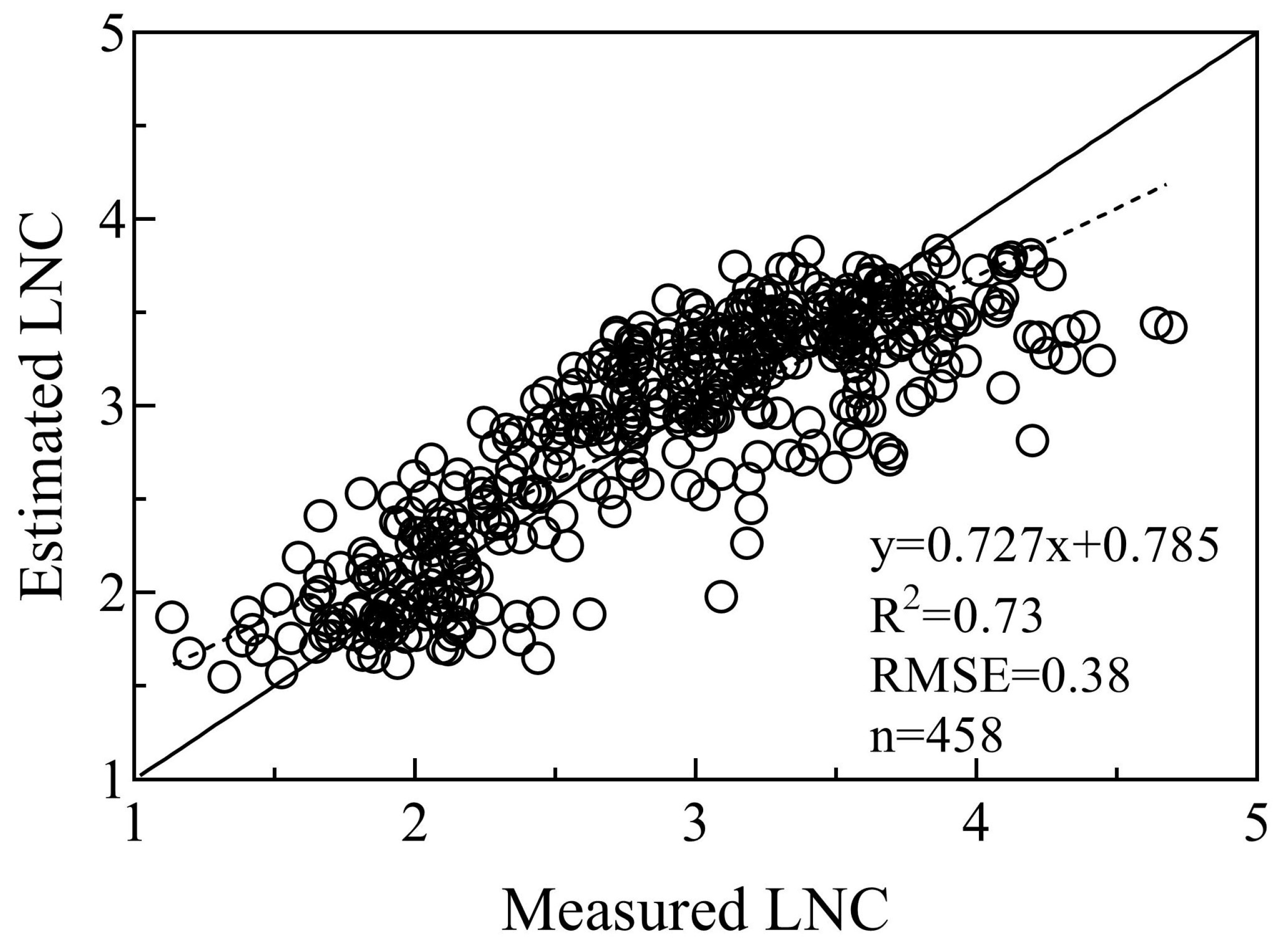
3.1. Optimal VI Determination

Relationships between LNC and 19 different formulas with random bands were established, and the best-performing VIs in each case are listed in

Table 6. Cross-validation statistics and processing speed for the best-performing vegetation index (VI) under each formulation.

	VI	Optimal Bands	R2	RMSE (%)	Processing Speed (s)
Two-band	RVI	λ1: 700; λ2: 800	0.49	0.52	0.029
	DVI	λ1: 800; λ2: 700	0.67	0.41	0.029
	NDVI	λ1: 800; λ2: 700	0.49	0.52	0.046
	RDVI	λ1: 800; λ2: 700	0.73	0.38	0.029
	SAVI	λ1: 800; λ2: 700	0.73	0.38	0.030
	OSAVI	λ1: 800; λ2: 671	0.70	0.40	0.029
	VIopt	λ1: 800; λ2: 671	0.69	0.40	0.029
	MSR	λ1: 700; λ2: 800	0.48	0.52	0.028
Three-band	EVI	λ1: 800; λ2: 700; λ3: 490	0.73	0.38	0.031
	mND	λ1: 800; λ2: 700; λ3: 490	0.69	0.40	0.029
	mSR	λ1: 700; λ2: 490; λ3: 800	0.68	0.41	0.026
	MCARI	λ1: 550; λ2: 700; λ3: 800	0.69	0.41	0.029
	TCARI	λ1: 550; λ2: 700; λ3: 800	0.68	0.41	0.028
	TBI1	λ1: 671; λ2: 700; λ3: 550	0.56	0.48	0.028
	TBI2	λ1: 800; λ2: 490; λ3: 671	0.55	0.49	0.028
Four-band	VOG	λ1: 490; λ2: 700; λ3: 800; λ4: 671	0.70	0.40	0.027
	MTCI	λ1: 671; λ2: 800; λ3: 700; λ4: 490	0.69	0.40	0.027
	TCARI/OSAVI	λ1: 550; λ2: 700; λ3: 800; λ4: 490	0.66	0.42	0.028
	MCARI/OSAVI	λ1: 550; λ2: 700; λ3: 800; λ4: 490	0.66	0.42	0.028

The row in bold type denotes the best-performing VI.

. Results show that both RDVI and SAVI performed equally well in the case of two-band indices (R² = 0.73 and RMSE = 0.38, respectively), outperforming other examples. In addition, optimal VI values for each formulation comprising two bands were constructed with a red edge (720 nm) and a near infrared band (800 nm); results show that EVI was superior to others in terms of LNC estimation in the case of three-band indices yielding an R² and RMSE of 0.73 and 0.38, respectively. Data show that all four-band indices exhibited similar LNC estimation efficiency even when encompassing different band combinations, but performed worse than optimal two-band and three-band VI variations. It is also clear that formulation type exerts a significant influence on VI performance even when the same bands are employed. In addition, this modeling method is characterized with an extremely fast speed (within 0.05 s) under the MATLAB. From the scatter plots shown in Figure 2, the saturation at high LNC values still exists despite a relatively high R², resulting in low estimation accuracy at high values.

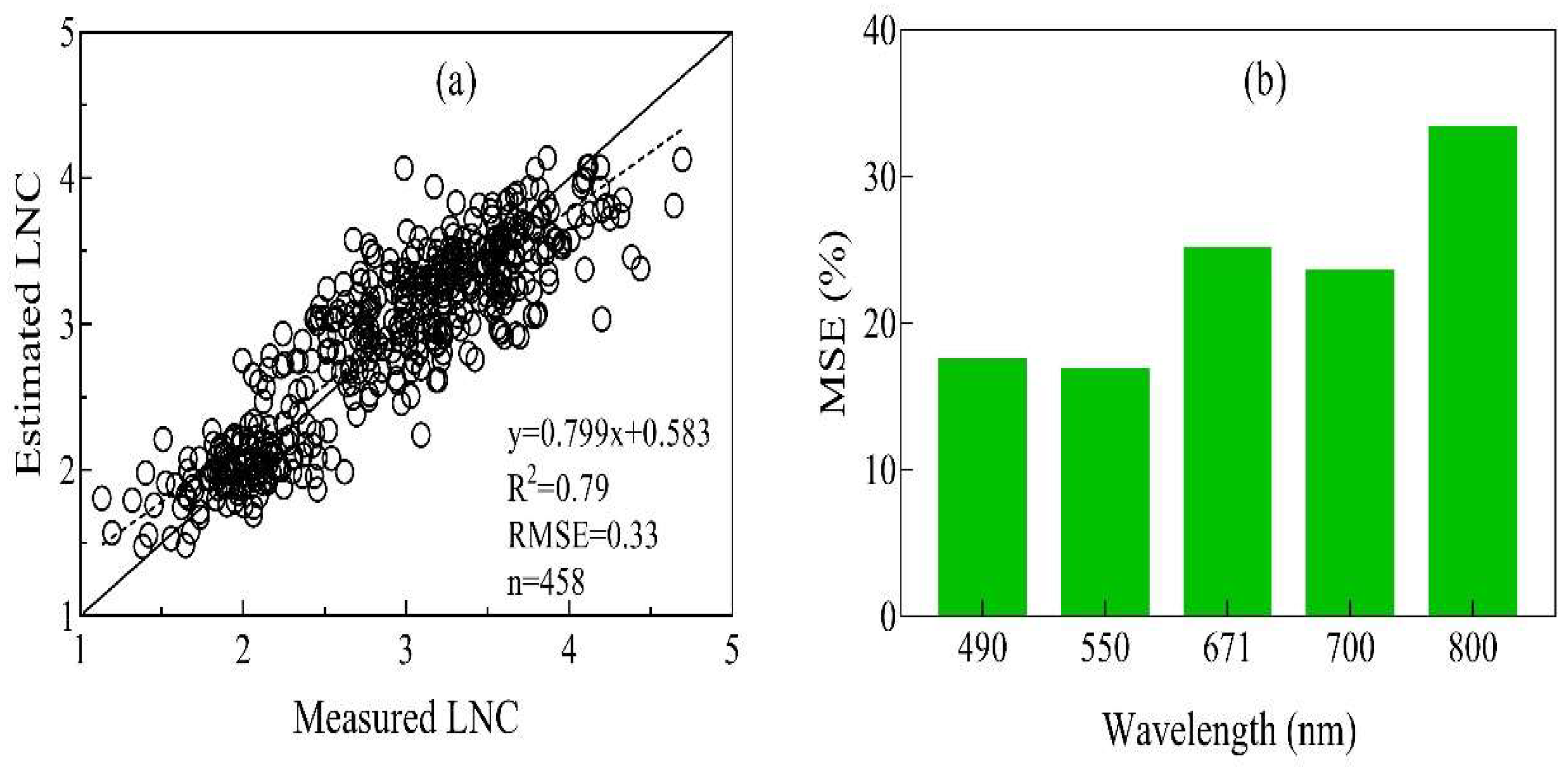
3.2. Optimal Non-Parametric Modeling Algorithm Determination

A total of 13 non-parametric modeling algorithms were utilized in this study to estimate wheat LNC (

Table 7. Performance of different non-parametric modeling algorithms in LNC estimation ranked according to RMSE values.

Non-Parametric Algorithm	R2	RMSE (%)	Processing Speed (s)
Random Forest (RF)	0.79	0.33	2.284
Bagging Trees (BaT)	0.78	0.34	2.700
Kernel Ridge Regression (KRR)	0.78	0.35	1.934
Neural Network (NN)	0.77	0.35	10.406
VH Gaussian Process Regression (VH-GPR)	0.77	0.35	17.059
Gaussian Process Regression (GPR)	0.77	0.35	4.265
Extreme Learning Machine (ELM)	0.76	0.36	20.068
Least-Squares Linear Regression (LSLR)	0.75	0.36	0.007
Boosting Trees (BoT)	0.75	0.37	2.301
Relevance Vector Machine (RVM)	0.75	0.37	268.473
Partial Least-Squares Regression (PLSR)	0.74	0.37	0.016
Principal Component Regression (PCR)	0.73	0.38	0.009
Regression Trees (RT)	0.69	0.40	0.616

); data show that all outperformed optimal VI, with the exception of RT. Indeed, the best-performing regression method was RF, which yielded an R² of 0.79 and an RMSE of 0.33 and had a fast processing speed of 2.28 s. In addition, we found that the majority of nonlinear non-parametric modeling algorithms were superior to their linear counterparts. Albeit yielding accurate estimates, RVM, ELM, VH-GPR, and NN approaches all proceeded very slowly. In contrast, the linear non-parametric regression models of LSLR, PCR, and PLSR were all extremely fast, more rapid even than their parametric counterparts.

The data presented in Figure 3a comprise scatter plots of measured LNC values versus estimated ones derived from the optimal non-parametric RF algorithm. In this case, estimated values at the high level turned out to be closer to the 1:1 line than those generated from RDVI. Thus, after measuring the importance of predictor variables using the mean squared error (MSE) [50], it is clear that these values for NIR (800 nm) bands were the largest among the five, followed by the red (671 nm) band (Figure 3b). The red (671 nm) and NIR (800 nm) bands are therefore more important for LNC estimation than any of their counterparts.

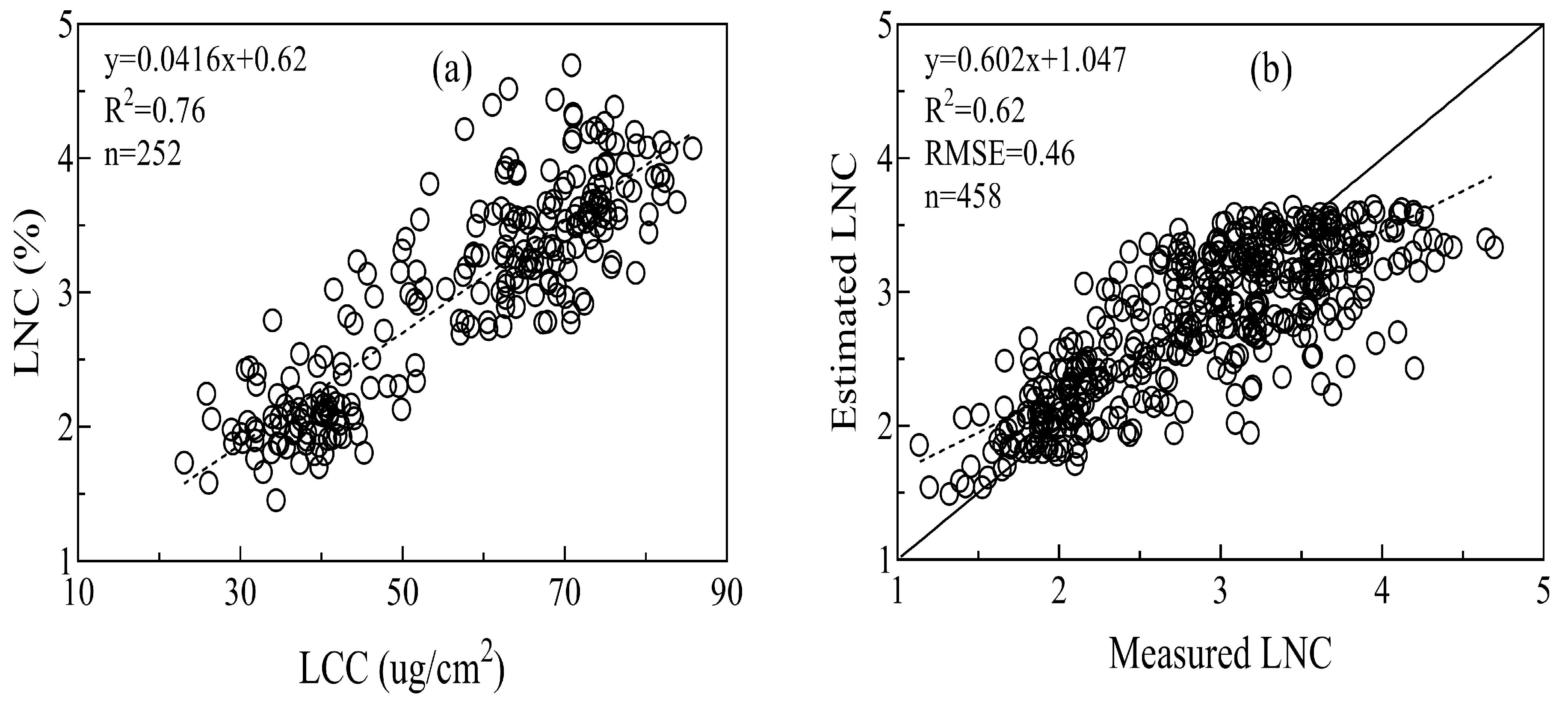
3.3. Performance of LUT-Based PROSAIL Inversion Performance

The data presented in

Table 8. Performance of different regularization strategies used in the PROSAIL model ranked according to RMSE values.

Cost Function	Noise (%)	Multiple Solutions (%)	R2	RMSE (μg/cm2)	Processing Speed (s)
K(x) = log(x)2	29	9	0.81	7.05	2.04
K(x) = x(log(x)) − x	41	41.5	0.75	8.24	1.85
Neyman chi-square	37	10.5	0.74	8.74	1.86
W Kagan	37	10.5	0.74	8.74	1.85
Kullback-Leibler	45	11.5	0.81	8.98	1.92
Jeffreys-Kullback-Leibler	45	19.5	0.80	9.17	1.76
Bhattacharyya divergence	45	19.5	0.81	9.26	2.03
Pearson chi-square	50	43	0.78	9.33	1.85
L-divergence Lin	47	20.5	0.81	9.35	2.16
Shannon (1948)	47	20.5	0.81	9.35	1.98
Shannon entropy	50	21.5	0.81	9.45	1.82
Harmonique toussaint	50	21	0.81	9.50	1.85
K-divergence Lin	50	30.5	0.80	9.54	1.96
Negative exponential disparity	48	20.5	0.79	9.65	1.92
Exponential	50	48	0.59	11.84	1.98
Normal distribution-LSE	50	50	0.47	13.10	1.74
Geman and McClure	50	50	0.46	13.16	1.79
K(x) = −log(x) + x	39	50	0.79	13.19	1.98
Least absolute error	50	50	0.34	15.16	1.75
K(x) = log(x) + 1/x	50	50	0.07	17.61	1.96

illustrate the performance of the LUT-based PROSAIL model with different cost functions, noise proportions, and multiple solutions. In this case, however, as LNC could not be retrieved directly from the PROSAIL model, LCC was initially estimated. The optimal inversion strategy for LCC retrieval used in this study was K(x) = log(x)² with R² and RMSE values of 0.81 and 7.05, respectively. LNC was then indirectly estimated subsequent to LCC inversion via the relationship between LCC and LNC (Figure 4a). The PROSAIL model performance in LNC inversion was not particularly satisfactory with an R² value of 0.62 (Figure 4b); thus, compared to both VIs and non-parameter modeling methods, the LUT-based PROSAIL approach actually performed worse although the processing speed in this case was comparable with those of non-linear non-parametric regression algorithms.

3.4. Effects of Growth Stage, Cultivar, and Cultivation Factors on Estimation Accuracy

The data presented in

Table 9. Relative RMSE (RRMSE, %) values for different wheat LNC estimation methods under different conditions.

Sub-Group	Treatment	Different Modeling Algorithms
		RDVI	RF	LUT
Growth stage	Jointing	16.0	11.4	16.53
	Booting	8.8	8.8	12.60
	Heading	10.0	9.9	12.80
	Anthesis	11.7	11.7	14.03
	Filling	17.9	16.2	22.92
Variety	Yangmai 18	13.1	11.3	16.34
	Shengxuan 6	14.0	12.0	16.43
	Xumai 30	13.4	11.9	16.51
	Ningmai 13	10.4	10.7	15.41
Plant density	1.5 × 106 plants/ha	12.1	12.1	13.41
	2.4 × 106 plants/ha	12.4	11.7	16.30
	3 × 106 plants/ha	14.4	11.1	16.34
Year	2014	12.0	11.2	0.14
	2015	14.6	12.2	0.18

summarize the effects of growth stage, cultivar, planting density, and year on the estimation accuracy of different methods. These records show that for different growth stages, both RDVI and LUT-based methods performed better in the middle of the season (i.e., booting, heading, and anthesis) compared to either early (i.e., jointing) or late (filling) stages. An RF approach was able to obtain accurate estimates from jointing to anthesis stages alongside lower ones at the filling stage.

The results of this study reveal varied RDVI performance depending on the wheat cultivar; the most accurate estimates were recovered for Ningmai 13 (RRMSE = 10.4%) while the worst were seen for Shenxuan 6 (RRMSE = 14.0%). The RF approach also generated satisfactory and stable values for different cultivars with RRMSE ranging between 10.7% and 12.0%, while the LUT-based retrieval method also performed equally in all cases.

As planting density increased, LNC estimation accuracy gradually decreased based on RDVI and the best performance was obtained at the lowest density. At the same time, the LUT-based retrieval method yielded highest accuracies at the lowest density while the RF approach led to comparable performance at different planting densities. All three methods performed better for 2014 than for 2015.

4. Discussion

Although ground-based spectral data and satellite images have been widely utilized to monitor the N status of crops [9,16,51], few studies to date have assessed the capabilities of UAV platforms. We evaluated the performance of UAV images using different modeling algorithms and demonstrate that this approach provides a reliable technique for winter wheat leaf N content estimation.

The results of this analysis show that in terms of parametric approaches, use of an RDVI modified with NIR and red edge bands provides optimal VI values for LNC estimation (i.e., R² = 0.73; RMSE = 0.38); this result is in close agreement with the previous findings of Inoue et al. [20] and Yao et al. [52], who noted that a combination of NIR and red edge bands provides an efficient approach for N status monitoring. The RDVI is also advantageous because it optimizes the vegetation signal and therefore has an improved degree of sensitivity in high-biomass regions; this approach is able to enhance vegetation monitoring via decoupling of the canopy background signal and reducing atmospheric influence [38].

However, even though results of sufficient accuracy were obtained in this analysis using a simple model, a number of drawbacks remain, including the fact that this approach becomes saturated at high N rates and canopy densities; it is easily affected by the growth stage, and information is lost at other spectral bands. Indeed, the RDVI performed poorly at both jointing and filling stages (Table 8), a result that might be explained by the fact that the canopy was mixed with soil background during the early stage and then panicles later in development. Furthermore, the accuracy of estimation decreased from the booting to filling stage, which might be due to the differences of the leaf biomass at varied stages [53]. The use of the VI incorporating more bands was also unable to generate higher accuracy than a two-band approach; furthermore, different formulas with the same bands performed significantly in LNC estimation, which indicated that both band configuration and VI formulation played an important role in LNC estimation. It is also crucial to consider the applicability of VI-LNC models as the performance of these approaches often depends on the ecological site, crop type, and growth stage [54]. The RDVI-LNC model should therefore be tested using additional datasets so as to extend its capability in the future.

It is well known that vegetation canopy spectral signatures are dominated by numerous biophysical and biochemical variables [55,56]. Thus, compared with parametric methods, most non-parametric algorithms tend to perform better because this regression family makes full use of all spectral information and so are able to better handle confounding factors when compared to VI values [20,22]. Although linear non-parametric algorithms performed lightly worse than their nonlinear counterparts in this analysis, these approaches possessed an extremely fast processing speed; this attribute indicates that these methods comprise a promising technique that can be integrated into crop monitoring systems.

Previous studies have also shown that linear non-parametric algorithms, such as PLSR, are able to generate satisfactory estimates for crop biomass [3] as well as N [20] and chlorophyll content [22]. The results of this study show that amongst non-parametric algorithms, the RF approach was both the most accurate and stable method under different conditions because RF provides a nonlinear regression with LNC and has the advantage of dealing with a large dataset with high speed and efficiency [50,57]. Furthermore, RF also has the ability to rank the importance of variables [50,57]. We therefore recommend that the RF approach would be a reliable technique for crop N estimation, even though many software packages do not yet include this algorithm.

The LUT-based retrieval method used in this study had the lowest LNC estimation accuracy of the three approaches tried, in contrast to previous research results [27,58]. Indeed, as some variables (e.g., LAI and chlorophyll content) could be retrieved directly from the PROSAIL model while LNC was generated indirectly from the empirical relationship between LNC and LCC [59,60], estimation accuracy was influenced by retrieval equation accuracy. We also note that the LUT-based retrieval method has a number of drawbacks, including the need for too many input parameters, large data size, and long processing times, and the fact that only parameters inherent to the model can be retrieved. However, a physical model has the advantage of offering uncertainty estimates, which provide information on model transplantation possibilities.

Although previous studies have attempted to employ UAV-based images to monitor crop N status [14,15], the datasets used was small and so estimation accuracy was unsatisfactory. In contrast, the results of this study show that the RDVI generated higher estimates while the non-parametric RF regression method led to a higher degree of accuracy under different conditions. These results suggest that UAV-based multispectral images provide a promising approach that can be applied to crop N status monitoring. However, even though a high predictive accuracy was obtained in this study, the established LNC model will still need to be tested with data from other ecological sites and crop types as the variables used here came from just one site. We also show that the PROSAIL model is not suitable for LNC retrieval because of its low predictive accuracy unless the relationship between this variable and LNC can be made more robust.

5. Conclusions

A range of modeling algorithms (i.e., parametric, non-parametric, and physical retrieval) were employed in this study to estimate winter wheat LNC using UAV-based multispectral images. Estimation models were then cross-validated with datasets from different growing seasons, including different stages, cultivars, N rates, and planting densities. In terms of parametric regressions, modified RDVI with a red edge and NIR bands turned out to comprise the best-performing index with the most accurate cross-validated result (i.e., R² = 0.73, RMSE = 0.38). This method was also characterized by an extremely high processing speed and a saturation effect at high LNC levels. In terms of non-parametric regression approaches, we showed that the RF method comprised the best-performing algorithm (i.e., R² = 0.79, RMSE = 0.33), also with a fast processing speed. The use of a physical retrieval method remains challenging for LNC estimations because of undeterminable input variables and low prediction accuracies.

References

1. Hatfield, J.L.; Gitelson, A.A.; Schepers, J.S.; Walthall, C.L. Application of spectral remote sensing for agronomic decisions. Agron. J. 2008, 100, 117–131. [Google Scholar] [CrossRef]
2. Ju, X.T.; Xing, G.X.; Chen, X.P.; Zhang, S.L.; Zhang, L.J.; Liu, X.J.; Cui, Z.L.; Yin, B.; Christie, P.; Zhu, Z.L.; et al. Reducing environmental risk by improving N management in intensive Chinese agricultural systems. Proc. Natl. Acad. Sci. USA 2009, 106, 3041–3046. [Google Scholar] [CrossRef] [PubMed] [Green Version]
3. Hansen, P.M.; Schjoerring, J.K. Reflectance measurement of canopy biomass and nitrogen status in wheat crops using normalized difference vegetation indices and partial least squares regression. Remote Sens. Environ. 2003, 86, 542–553. [Google Scholar] [CrossRef]
4. Tan, C.; Guo, W.; Wang, J. Predicting grain protein content of winter wheat based on Landsat TM images and leaf nitrogen content. In Proceedings of the International Conference on Remote Sensing, Environment and Transportation Engineering, Nanjing, China, 24–26 June 2011. [Google Scholar]
5. Eitel, J.U.H.; Long, D.S.; Gessler, P.E.; Smith, A.M.S. Using in-situ measurements to evaluate the new RapidEyeTM satellite series for prediction of wheat nitrogen status. Int. J. Remote Sens. 2007, 28, 4183–4190. [Google Scholar] [CrossRef]
6. Huang, S.; Miao, Y.; Yuan, F.; Gnyp, M.L.; Yao, Y.; Cao, Q.; Wang, H.; Lenz-Wiedemann, V.I.; Bareth, G. Potential of RapidEye and WorldView-2 satellite data for improving rice nitrogen status monitoring at different growth stages. Remote Sens. 2017, 9, 227. [Google Scholar] [CrossRef]
7. Boegh, E.; Soegaard, H.; Broge, N.; Hasager, C.B.; Jensen, N.O.; Schelde, K.; Thomsen, A. Airborne multispectral data for quantifying leaf area index, nitrogen concentration, and photosynthetic efficiency in agriculture. Remote Sens. Environ. 2002, 81, 179–193. [Google Scholar] [CrossRef]
8. Tian, Y.C.; Yao, X.; Yang, J.; Cao, W.X.; Hannaway, D.B.; Zhu, Y. Assessing newly developed and published vegetation indices for estimating rice leaf nitrogen concentration with ground-and space-based hyperspectral reflectance. Field Crops Res. 2011, 120, 299–310. [Google Scholar] [CrossRef]
9. Yao, X.; Ren, H.; Cao, Z.; Tian, Y.; Cao, W.; Zhu, Y.; Cheng, T. Detecting leaf nitrogen content in wheat with canopy hyperspectrum under different soil backgrounds. Int. J. Appl. Earth Obs. Geoinf. 2014, 32, 114–124. [Google Scholar] [CrossRef]
10. Bendig, J.; Yu, K.; Aasen, H.; Bolten, A.; Bennertz, S.; Broscheit, J.; Gnyp, M.L.; Bareth, G. Combining UAV-based plant height from crop surface models, visible, and near infrared vegetation indices for biomass monitoring in barley. Int. J. Appl. Earth Obs. Geoinf. 2015, 39, 79–87. [Google Scholar] [CrossRef]
11. Zheng, H.; Cheng, T.; Li, D.; Zhou, X.; Yao, X.; Tian, Y.; Cao, W.; Zhu, Y. Evaluation of RGB, color-infrared and multispectral images acquired from unmanned aerial systems for the estimation of nitrogen accumulation in rice. Remote Sens. 2018, 10, 824. [Google Scholar] [CrossRef]
12. Yao, X.; Wang, N.; Liu, Y.; Cheng, T.; Tian, Y.; Chen, Q.; Zhu, Y. Estimation of wheat LAI at middle to high levels using unmanned aerial vehicle narrowband multispectral imagery. Remote Sens. 2017, 9, 1304. [Google Scholar] [CrossRef]
13. Yue, J.; Yang, G.; Li, C.; Li, Z.; Wang, Y.; Feng, H.; Xu, B. Estimation of winter wheat above-ground biomass using unmanned aerial vehicle-based snapshot hyperspectral sensor and crop height improved models. Remote Sens. 2017, 9, 708. [Google Scholar] [CrossRef]
14. Gnyp, M.L.; Panitzki, M.; Reusch, S.; Jasper, J.; Bolten, A.; Bareth, G. Comparison between tractor -based and UAV-based spectrometer measurements in winter wheat. In Proceedings of the 13th International Conference on Precision Agriculture, Monticello, IL, USA, 31 July–3 August 2016. [Google Scholar]
15. Li, J.; Zhang, F.; Qian, X.; Zhu, Y.; Shen, G. Quantification of rice canopy nitrogen balance index with digital imagery from unmanned aerial vehicle. Remote Sens. Lett. 2015, 6, 183–189. [Google Scholar] [CrossRef]
16. Stroppiana, D.; Boschetti, M.; Brivio, P.A.; Bocchi, S. Plant nitrogen concentration in paddy rice from field canopy hyperspectral radiometry. Field Crops Res. 2009, 111, 119–129. [Google Scholar] [CrossRef]
17. Wang, W.; Yao, X.; Yao, X.; Tian, Y.; Liu, X.; Ni, J.; Cao, W.; Zhu, Y. Estimating leaf nitrogen concentration with three-band vegetation indices in rice and wheat. Field Crops Res. 2012, 129, 90–98. [Google Scholar] [CrossRef]
18. Rivera, J.P.; Verrelst, J.; Delegido, J.; Veroustraete, F.; Moreno, J. On the semi-automatic retrieval of biophysical parameters based on spectral index optimization. Remote Sens. 2014, 6, 4927–4951. [Google Scholar] [CrossRef]
19. Zhu, Y.; Tian, Y.; Yao, X.; Liu, X.; Cao, W. Analysis of common canopy reflectance spectra for indicating leaf nitrogen concentrations in wheat and rice. Plant Prod. Sci. 2007, 10, 400–411. [Google Scholar] [CrossRef]
20. Inoue, Y.; Sakaiya, E.; Zhu, Y.; Takahashi, W. Diagnostic mapping of canopy nitrogen content in rice based on hyperspectral measurements. Remote Sens. Environ. 2012, 126, 210–221. [Google Scholar] [CrossRef]
21. Yao, X.; Huang, Y.; Shang, G.; Zhou, C.; Cheng, T.; Tian, Y.; Cao, W.; Zhu, Y. Evaluation of six algorithms to monitor wheat leaf nitrogen concentration. Remote Sens. 2015, 7, 14939–14966. [Google Scholar] [CrossRef]
22. Atzberger, C.; Guérif, M.; Baret, F.; Werner, W. Comparative analysis of three chemometric techniques for the spectroradiometric assessment of canopy chlorophyll content in winter wheat. Comput. Electron. Agric. 2010, 73, 165–173. [Google Scholar] [CrossRef]
23. Verrelst, J.; Muñoz, J.; Alonso, L.; Delegido, J.; Rivera, J.P.; Camps-Valls, G.; Moreno, J. Machine learning regression algorithms for biophysical parameter retrieval: Opportunities for Sentinel-2 and-3. Remote Sens. Environ. 2012, 118, 127–139. [Google Scholar] [CrossRef]
24. Jacquemoud, S.; Baret, F.; Andrieu, B.; Danson, F.M.; Jaggard, K. Extraction of vegetation biophysical parameters by inversion of the PROSPECT + SAIL models on sugar beet canopy reflectance data. Application to TM and AVIRIS sensors. Remote Sens. Environ. 1995, 52, 163–172. [Google Scholar] [CrossRef]
25. Liang, L.; Di, L.; Zhang, L.; Deng, M.; Qin, Z.; Zhao, S.; Lin, H. Estimation of crop LAI using hyperspectral vegetation indices and a hybrid inversion method. Remote Sens. Environ. 2015, 165, 123–134. [Google Scholar] [CrossRef]
26. Yang, G.; Zhao, C.; Xing, Z.; Huang, W.; Wang, J. LAI Inversion of Spring Wheat Based on PROBA/CHRIS Hyperspectral Multi-Angular Data and PROSAIL Model. Available online: http://xueshu.baidu.com/usercenter/paper/show?paperid=7ff0cdf37366c37dd6406bf9aa80a99f&site=xueshu_se&hitarticle=1 (accessed on 11 December 2018).
27. Botha, E.J.; Leblon, B.; Zebarth, B.; Watmough, J. Non-destructive estimation of potato leaf chlorophyll from canopy hyperspectral reflectance using the inverted PROSAIL model. Int. J. Appl. Earth Obs. Geoinf. 2007, 9, 360–374. [Google Scholar] [CrossRef]
28. Uddling, J.; Gelang-Alfredsson, J.; Piikki, K.; Pleijel, H. Evaluating the relationship between leaf chlorophyll concentration and SPAD-502 chlorophyll meter readings. Photosynth. Res. 2007, 91, 37–46. [Google Scholar] [CrossRef]
29. Kelcey, J.; Lucieer, A. Sensor correction of a 6-band multispectral imaging sensor for UAV remote sensing. Remote Sens. 2012, 4, 1462–1493. [Google Scholar] [CrossRef]
30. Smith, G.M.; Milton, E.J. The use of the empirical line method to calibrate remotely sensed data to reflectance. Int. J. Remote Sens. 1999, 20, 2653–2662. [Google Scholar] [CrossRef]
31. Jordan, C.F. Derivation of leaf area index from quality of light on the forest floor. Ecology 1969, 50, 663–666. [Google Scholar] [CrossRef]
32. Tucker, C.J. Red and photographic infrared linear combinations for monitoring vegetation. Remote Sens. Environ. 1979, 8, 127–150. [Google Scholar] [CrossRef] [Green Version]
33. Roujean, J.L.; Breon, F.M. Estimating PAR absorbed by vegetation from bidirectional reflectance measurements. Remote Sens. Environ. 1995, 51, 375–384. [Google Scholar] [CrossRef]
34. Huete, A.R. A soil-adjusted vegetation index (SAVI). Remote Sens. Environ. 1988, 25, 295–309. [Google Scholar] [CrossRef]
35. Rondeaux, G.; Steven, M.; Baret, F. Optimization of soil-adjusted vegetation indices. Remote Sens. Environ. 1996, 55, 95–107. [Google Scholar] [CrossRef]
36. Reyniers, M.; Walvoort, D.J.; De Baardemaaker, J. A linear model to predict with a multi-spectral radiometer the amount of nitrogen in winter wheat. Int. J. Remote Sens. 2006, 27, 4159–4179. [Google Scholar] [CrossRef]
37. Chen, J.M. Evaluation of vegetation indices and a modified simple ratio for boreal applications. Can. J. Remote Sens. 1996, 22, 229–242. [Google Scholar] [CrossRef]
38. Huete, A.; Didan, K.; Miura, T.; Rodriguez, E.P.; Gao, X.; Ferreira, L.G. Overview of the radiometric and biophysical performance of the MODIS vegetation indices. Remote Sens. Environ. 2002, 83, 195–213. [Google Scholar] [CrossRef]
39. Sims, D.A.; Gamon, J.A. Relationships between leaf pigment content and spectral reflectance across a wide range of species, leaf structures and developmental stages. Remote Sens. Environ. 2002, 81, 337–354. [Google Scholar] [CrossRef]
40. Daughtry, C.S.T.; Walthall, C.L.; Kim, M.S.; De Colstoun, E.B.; McMurtrey Iii, J.E. Estimating corn leaf chlorophyll concentration from leaf and canopy reflectance. Remote Sens. Environ. 2000, 74, 229–239. [Google Scholar] [CrossRef]
41. Haboudane, D.; Miller, J.R.; Tremblay, N.; Zarco-Tejada, P.J.; Dextraze, L. Integrated narrow-band vegetation indices for prediction of crop chlorophyll content for application to precision agriculture. Remote Sens. Environ. 2002, 81, 416–426. [Google Scholar] [CrossRef]
42. Tian, Y.C.; Gu, K.J.; Chu, X.; Yao, X.; Cao, W.X.; Zhu, Y. Comparison of different hyperspectral vegetation indices for canopy leaf nitrogen concentration estimation in rice. Plant Soil 2014, 376, 193–209. [Google Scholar] [CrossRef]
43. Zarco-Tejada, P.J.; Miller, J.R.; Noland, T.L.; Mohammed, G.H.; Sampson, P.H. Scaling-up and model inversion methods with narrowband optical indices for chlorophyll content estimation in closed forest canopies with hyperspectral data. IEEE Trans. Geosci. Remote Sens. 2001, 39, 1491–1507. [Google Scholar] [CrossRef] [Green Version]
44. Dash, J.; Curran, P.J. The MERIS terrestrial chlorophyll index. Int. J. Remote Sens. 2004, 25, 5403–5413. [Google Scholar] [CrossRef]
45. Camps-Valls, G.; Gómez-Chova, L.; Muñoz-Marí, J.; Lázaro-Gredilla, M.; Verrelst, J. simpleR: A Simple Educational Matlab Toolbox for Statistical Regression. In: V2. Available online: https://www.uv.es/gcamps/software.html (accessed on 10 December 2018).
46. Verrelst, J.; Rivera, J.P.; Veroustraete, F.; Muñoz-Marí, J.; Clevers, J.G.; Camps-Valls, G.; Moreno, J. Experimental Sentinel-2 LAI estimation using parametric, non-parametric and physical retrieval methods-A comparison. ISPRS J. Photogramm. Remote Sens. 2015, 108, 260–272. [Google Scholar] [CrossRef]
47. Zhang, L.; Guo, C.L.; Zhao, L.Y.; Zhu, Y.; Cao, W.X.; Tian, Y.C.; Cheng, T.; Wang, X. Estimating wheat yield by integrating the WheatGrow and PROSAIL models. Field Crops Res. 2016, 192, 55–66. [Google Scholar] [CrossRef]
48. Li, H.; Liu, G.; Liu, Q.; Chen, Z.; Huang, C. Retrieval of winter wheat leaf area index from Chinese GF-1 satellite data using the PROSAIL model. Sensors 2018, 18, 1120. [Google Scholar] [CrossRef] [PubMed]
49. Rivera, J.P.; Verrelst, J.; Leonenko, G.; Moreno, J. Multiple cost functions and regularization options for improved retrieval of leaf chlorophyll content and LAI through inversion of the PROSAIL model. Remote Sens. 2013, 5, 3280–3304. [Google Scholar] [CrossRef]
50. Breiman, L. Random Forests. Mach. Learn. 2001, 45, 5–32. [Google Scholar] [CrossRef] [Green Version]
51. Huang, S.; Miao, Y.; Zhao, G.; Yuan, F.; Ma, X.; Tan, C.; Yu, W.; Gnyp, M.L.; Lenz-Wiedemann, V.I.; Rascher, U.; et al. Satellite remote sensing-based in-season diagnosis of rice nitrogen status in Northeast China. Remote Sens. 2015, 7, 10646–10667. [Google Scholar] [CrossRef]
52. Yao, X.; Zhu, Y.; Tian, Y.; Feng, W.; Cao, W. Exploring hyperspectral bands and estimation indices for leaf nitrogen accumulation in wheat. Int. J. Appl. Earth Obs. Geoinf. 2010, 12, 89–100. [Google Scholar] [CrossRef]
53. Li, F.; Gnyp, M.L.; Jia, L.; Miao, Y.; Yu, Z.; Koppe, W.; Zhang, F. Estimating N status of winter wheat using a handheld spectrometer in the North China Plain. Field Crops Res. 2008, 106, 77–85. [Google Scholar] [CrossRef]
54. Nigam, R.; Bhattacharya, B.K.; Vyas, S.; Oza, M.P. Retrieval of wheat leaf area index from AWiFS multispectral data using canopy radiative transfer simulation. Int. J. Appl. Earth Obs. Geoinf. 2014, 32, 173–185. [Google Scholar] [CrossRef]
55. Asner, G.P. Biophysical and biochemical sources of variability in canopy reflectance. Remote Sens. Environ. 1998, 64, 234–253. [Google Scholar] [CrossRef]
56. Ustin, S.L. Remote sensing of canopy chemistry. Proc. Natl. Acad. Sci. USA 2013, 10, 804–805. [Google Scholar] [CrossRef] [PubMed]
57. Belgiu, M.; Dragut, L. Random forest in remote sensing: A review of applications and future directions. ISPRS J. Photogramm. Remote Sens. 2016, 114, 24–31. [Google Scholar] [CrossRef]
58. Jiang, J.; Comar, A.; Burger, P.; Bancal, P.; Weiss, M.; Baret, F. Estimation of leaf traits from reflectance measurements: Comparison between methods based on vegetation indices and several versions of the PROSPECT model. Plant Methods 2018, 14, 23. [Google Scholar] [CrossRef] [PubMed]
59. Cammarano, D.; Fitzgerald, G.; Basso, B.; O’Leary, G.; Chen, D.; Grace, P.; Fiorentino, C. Use of the Canopy Chlorophyl Content Index (CCCI) for remote estimation of wheat nitrogen content in rainfed environments. Agron. J. 2011, 103, 1597–1603. [Google Scholar] [CrossRef]
60. Zhao, C.; Wang, Z.; Wang, J.; Huang, W.; Guo, T. Early detection of canopy nitrogen deficiency in winter wheat (Triticum aestivum L.) based on hyperspectral measurement of canopy chlorophyll status. N. Z. J. Crop Hortic. Sci. 2011, 39, 251–262. [Google Scholar] [CrossRef]
Figure 1. The UAV equipped with multispectral camera used in this study.
Remotesensing 10 02026 g001
Figure 2. Comparison between measured and estimated LNC values with the best performing VI.
Remotesensing 10 02026 g002
Figure 3. Comparison of measured and estimated LNC values derived using the RF modeling algorithm (a) and MSE values for this model at different spectral bands (b).
Remotesensing 10 02026 g003
Figure 4. Empirical linear relationship between LCC and LNC values (a). Measured versus estimated LNC values derived from the most effective LUT-based inversion scheme (Table 8) (b).
Remotesensing 10 02026 g004