Evaluation of Ground Surface Models Derived from Unmanned Aerial Systems with Digital Aerial Photogrammetry in a Disturbed Conifer Forest

Abstract

Detailed vertical forest structure information can be remotely sensed by combining technologies of unmanned aerial systems (UAS) and digital aerial photogrammetry (DAP). A key limitation in the application of DAP methods, however, is the inability to produce accurate digital elevation models (DEM) in areas of dense vegetation. This study investigates the terrain modeling potential of UAS-DAP methods within a temperate conifer forest in British Columbia, Canada. UAS-acquired images were photogrammetrically processed to produce high-resolution DAP point clouds. To evaluate the terrain modeling ability of DAP, first, a sensitivity analysis was conducted to estimate optimal parameters of three ground-point classification algorithms designed for airborne laser scanning (ALS). Algorithms tested include progressive triangulated irregular network (TIN) densification (PTD), hierarchical robust interpolation (HRI) and simple progressive morphological filtering (SMRF). Points were classified as ground from the ALS and served as ground-truth data to which UAS-DAP derived DEMs were compared. The proportion of area with root mean square error (RMSE) <1.5 m were 56.5%, 51.6% and 52.3% for the PTD, HRI and SMRF methods respectively. To assess the influence of terrain slope and canopy cover, error values of DAP-DEMs produced using optimal parameters were compared to stratified classes of canopy cover and slope generated from ALS point clouds. Results indicate that canopy cover was approximately three times more influential on RMSE than terrain slope.

1. Introduction

The emergence of three-dimensional remote sensing techniques such as aerial laser scanning (ALS) and digital aerial photogrammetry (DAP) have the ability to provide detailed structural information in the form of point clouds. Provided an adequate digital elevation model (DEM) can be extracted from point clouds, analysis techniques such as individual tree crown detection (ITCD) [1,2,3,4] and area-based analysis (ABA) [5,6,7] can be applied to estimate metrics related to forest structure. ABA metrics generated from the normalized vertical distribution of point clouds can be used to describe complex forest attributes such as timber volume, biomass and basal area from models established between sample field measurements such as tree height and diameter at breast height (DBH). Similar ALS derived structural metrics have also been shown to highlight various animal-habitat associations, useful in implementing effective conservation strategies [8,9].

Concurrent with the development of DAP analysis techniques has been the increased adoption of camera-equipped unmanned aerial systems (UAS). Originally developed for military operations [10], UASs have been rapidly adopted in a wide range of commercial markets. Recent adoption of Lithium-Ion battery technologies in consumer UASs enable greater power to weight ratios and thus flight duration and payload capacity [11]. In addition, the decreasing size, cost and increasing resolution of consumer-grade cameras [10,12] have driven such rapid UAS expansion. Systems specializing in quadcopter flight stability, previously restricted to military use, can now be paired with flight planning software capable of maintaining above ground level (AGL) altitude or terrain following [13]. By flying at lower altitudes than manned counterparts, UAS can capture imagery of higher quality and spatial resolution while reducing dependency on cloud conditions [14]. Moreover, the ease of deployment of UAS allow for frequent flights and therefore the ability to monitor highly dynamic vegetation compared to conventional remote sensing platforms such as aircraft and satellites [15,16].

The ability to provide continuous ground points under complex vegetated environments [17] has facilitated the commercial adoption of ALS techniques to model terrain and thus assess forest structure [18]. In contrast, the derivation of dense photogrammetric point clouds from aerial imagery is a relatively newer technology [19,20,21,22]. Photogrammetry, based on principles of stereo-photography, is the process of gathering 3-D structure from overlapping portions of adjacent two-dimensional images [23]. The extraction of vertical structure relies on the identification of common objects, known as tie-points, in overlapping images. Practical applications for aerial photogrammetry exist [24,25] however, prior to modern digital cameras and advanced computing technology, the creation of photogrammetric products relied on expert photogrammetrists in addition to a pre-existing network of visible tie-points with known coordinates [26]. Automatic tie-point extraction is now possible with the emergence of Structure from Motion (SfM) algorithms, facilitating a marked increase in image-based 3D data generation [27]. As a result, DAP approaches are increasingly being applied in natural resource applications; however, detection of the ground using DAP has principally been limited to non-forested landscapes, open forests with no understory, or plantations (

Table 1. Recent studies utilizing digital aerial photogrammetry divided into forest structure and ground detection.

Publication	Year	Aerial Platform	Location	Landcover Type	Forest Structure	Ground Detection
[28]	2018	MA *	Northern Alberta, Canada	Mixedwood, Boreal and Temperate	√
[29]	2018	UAS	Edmundston, New Brunswick, Canada	Hardwood dominated		√
[30]	2017	UAS	Otsu City, Shiga Prefecture, Japan	Evergreen coniferous	√	√
[31]	2017	UAS	Alcochete, Central Portugal	Pinus pinea plantation	√	√
[32]	2017	MA	Central Norway	Temperate, coniferous	√
[33]	2016	UAS	Central British Columbia, Canada	Young coniferous (<15 years since clearcut)	√
[34]	2016	UAS	Central Belgium	Pasture, arable fields without crops		√
[35]	2016	UAS	Edwards Plateau, Central Texas, USA	Savannah, undulating hills, evergreen	√	√
[36]	2015	MA	Central Cambodia	Evergreen, deciduous,	√
[37]	2014	UAS	Southern Tasmania, Australia	Landslide zone, exposed soil, short grass		√
[38]	2013	Helium Blimp	Central Texas, USA	Bedrock		√
[39]	2012	UAS	Southeast Tasmania, Australia	Scattered shrubs, Coastal marsh, erosion scarp		√
[40]	2012	UAS	Southern Alps, France	Landslide zone, bedrock, exposed soil		√
[41]	2008	MA	New Brunswick, Canada	Boreal forest	√
[42]	2004	MA	Southern Finland	Temperate, coniferous	√

* Manned Aircraft.

).

The analysis of 3D point cloud data typically involves the separation of bare-earth from vegetation object components. This allows the point cloud to be normalized according to height above ground, thus facilitating the measurement of three-dimensional forest metrics. This process will be referred to herein as ground classification. The accuracy of such classification varies according to surface variability [43,44]; therefore, a DEM generation workflow that accounts for these factors is necessary to ensure accurate estimates of forest structure. Both DAP and ALS point clouds provide accurate, continuous top-of-crown measurements however, the ability for DAP to describe forest structure decreases with distance below the canopy surface. Furthermore, DAP is prone to producing voids in the point cloud where trees found in matching photos may occlude each other [45]. The disparity of bare-earth coverage between ALS and DAP generally increases with canopy height [5]. Nevertheless, the low cost and increased repeatability of DAP relative to ALS, for stand-level applications, shows significant potential [27,29]. Recent studies indicate that accurate DEM generation from the unsupervised classification of DAP point clouds under open forest canopies is achievable [29,31,46,47]. For example Guerra-Hernández et al. [31] used 20 high precision GPS checkpoints and found RMSE of 0.046 m, 0.018 m and 0.033 m in the X, Y and Z directions respectively.

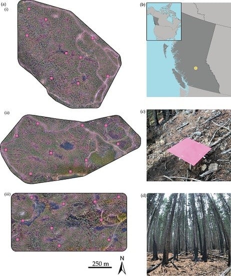
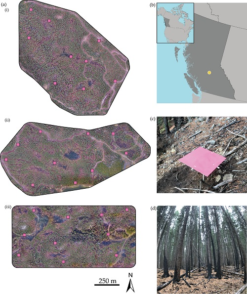
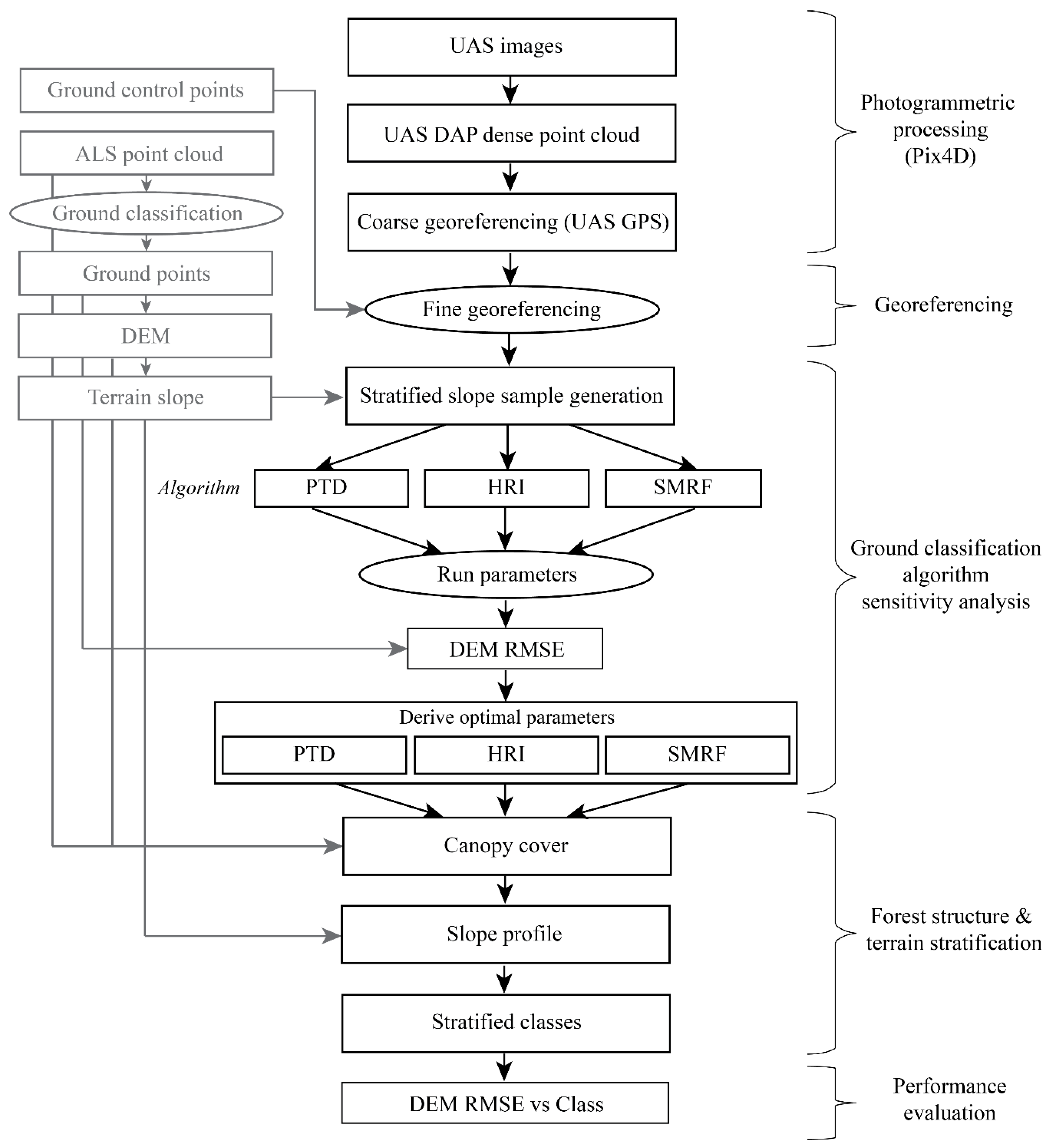
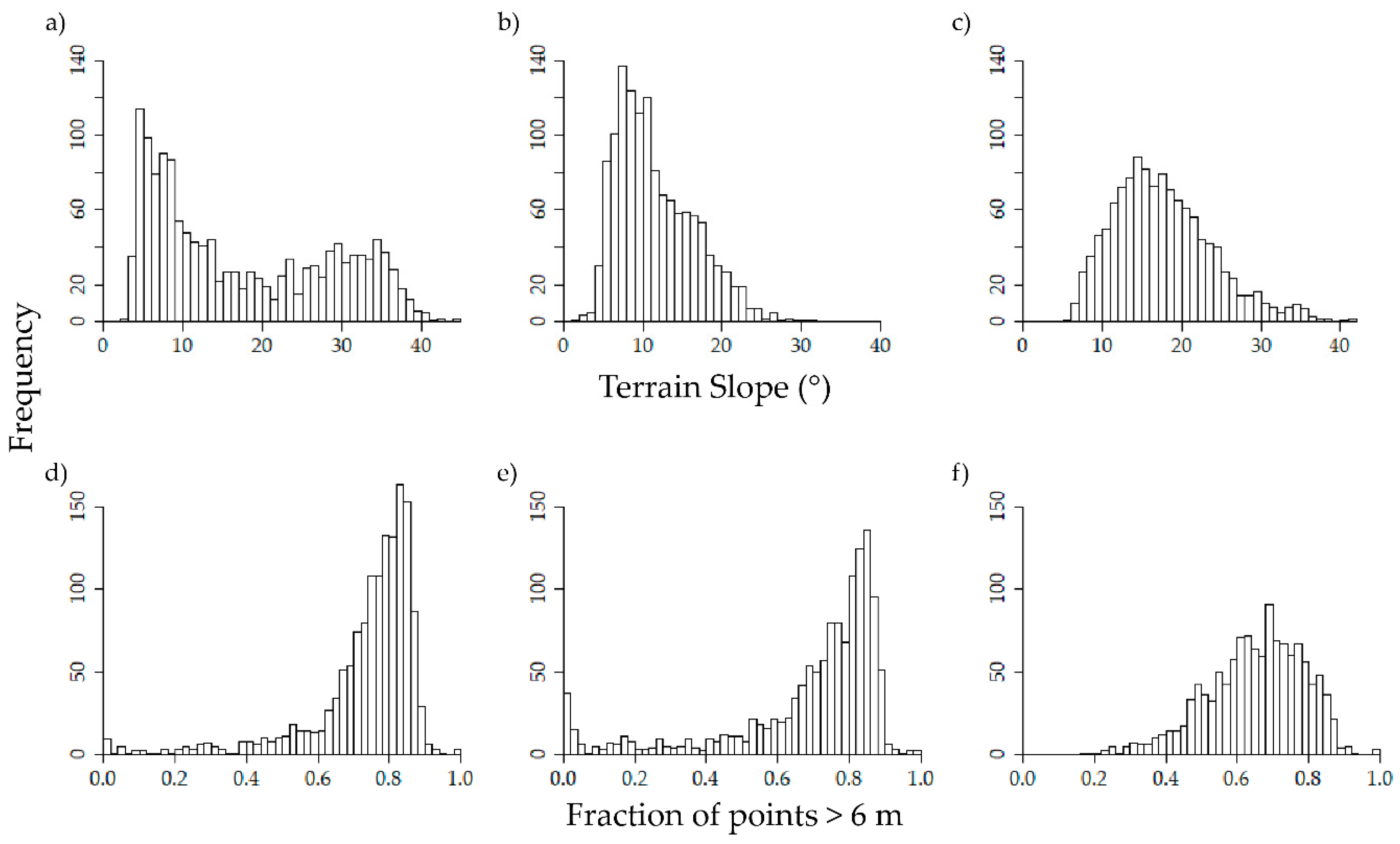
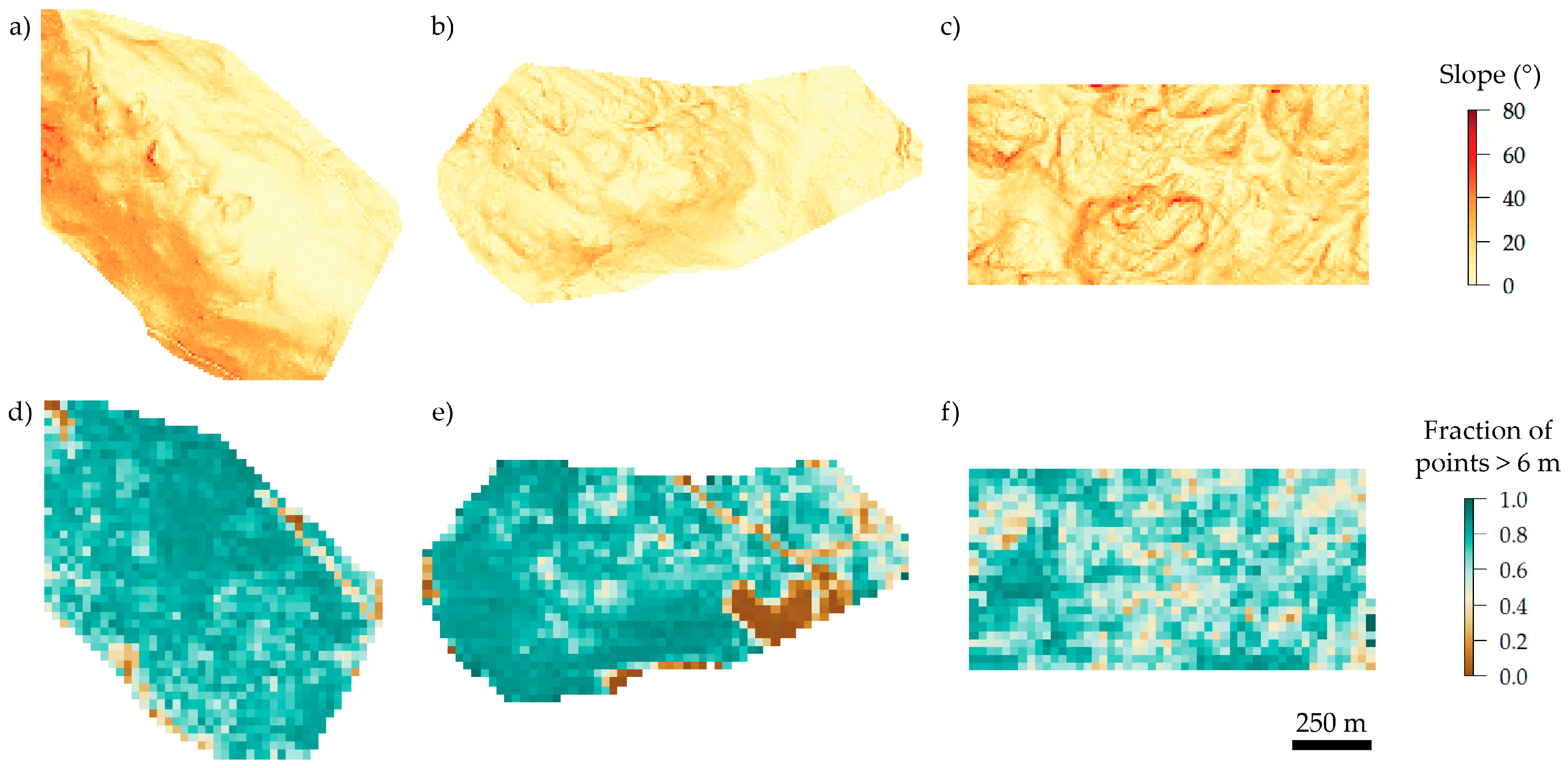
This study aims to (1) obtain terrain-modeling results typical of a low-cost UAS DAP acquisition in a mountainous forest environment, (2) establish optimal parameters of three ground-point classification algorithms, and (3) compare DAP terrain-modeling accuracies under various terrain slope and forest cover conditions. In this paper, we first outline the physical characteristics of the study area chosen for UAS DAP. Secondly, we present the DAP SfM point cloud processing chain and ground control point (GCP) based method of point cloud georeferencing used in this study. This is followed by a description of the ground-point filtering methods applied to UAS DAP point clouds, in addition to a surface interpolation method employed to generate all DEMs. A sensitivity analysis of the ground filtering methods is then described for the purpose of estimating optimal parameters. Accuracies of the UAS DAP derived DEMs (DAP-DEM) are then evaluated against ground filtered ALS points using root-mean-square error (RMSE) and the vertical residual distances (bias) across six stratified classes of forest canopy cover and terrain slope. Lastly, the relative influence of terrain slope and canopy cover on the DAP-DEM error are assessed using a random forest model. We conclude by proposing operational guidelines on the use of DAP to detect the ground surfaces in forest situations.

2. Materials and Methods

This study was carried out in five steps: photogrammetric processing, georeferencing, ground filter sensitivity analysis, forest structure and terrain stratification and performance evaluation. Figure 1 illustrates the conceptual workflow of the methodology. First, UAS images from three acquisitions were processed to generate photogrammetric point clouds. The point clouds were then georeferenced using GCPs followed by a systematic sensitivity analysis of three ground-point classification algorithms to determine optimal parameters, resulting in a single ground classified point cloud for each algorithm. Finally, performance evaluation was carried out to assess the accuracy of subsequently generated DEMs under various terrain slope and forest cover classes.

2.1. Study Area

DAP-DEM evaluations were conducted in three study areas (Figure 2) located within the University of British Columbia Alex Fraser Research Forest (AFRF) Gavin Lake Block, about 50 km northeast of Williams Lake, British Columbia, Canada. The block transitions west to east from the Sub-boreal Spruce (SBS) to the Interior Cedar Hemlock (ICH) biogeoclimatic ecosystem classification (BEC) zones. Forest structure of the Gavin Lake block is a product of frequent wildfires and logging activity dating back to the 1940’s [48]. The forest stands are dominated by coniferous with small patches of deciduous species [49]. Tree species in decreasing abundance are Douglas-fir (Psuedotsuga menziesii var. glauca (56%)), hybrid spruce (Picea glauca × engelmannii (15%)), western redcedar (Thuja plicata (10%)), lodgepole pine (Pinus contorta (9%)), and trembling aspen (Populus tremuloides (6%)) [49]. The combined areas lie between 700 m and 1250 m MSL with varying terrain slopes up to 68° and a mean slope of 16°. In addition to ALS data availability, sites were chosen to represent the variability of forest canopy density and terrain complexity of British Columbia’s interior plateau physiographic region.

A number of non-contiguous wildfires affected sizeable portions of the AFRF Gavin Lake Block with heterogeneous severity in the summer of 2017 prior to UAS data acquisition. As a result, portions of the study areas consist of dead or dying trees along with scorched ground and tree stems. Where the fire intensity was higher, any standing trees had reduced or completely removed foliage. These areas are identifiable in Figure 2 as patches of dark grey and black, where a visual estimation of aggregated burn area increases from area A to C. In order to quantify the proportional burned area within the study areas, relative differenced Normalized Burn Ratio (RdNBR) was divided into low, moderate and high fire severity classes from Landsat TM/ETM+ imagery as per Soverel et al. [50]. The proportion of fire severity classes across aggregated over the focus acquisitions was 28.9%, 14.5% and 5.4% for low, moderate and high respectively.

2.2. Image Acquisition

UAS DAP data acquisitions were conducted within the AFRF Gavin Lake block from 21 to 24 October 2017 using a DJI Phantom 4 quadcopter UAS equipped with a compact RGB digital camera. Each of the study areas (A, B and C) were flown on a single day with up to eight flights per area. Weather conditions were predominantly clear sky with minimal cloud coverage. No precipitation was observed during any acquisitions. The specifications of the phantom UAS along with employed acquisition parameters are presented in

Table 2. UAS specifications of the DJI Phantom 4 and parameters used for image acquisition.

System Specifications
Aircraft
Max Flight Time	28 min
Navigation	GPS & GLONASS
GPS Positional Accuracy	0.5 m (z), 1.5 m (x,y)
Transmission Range	5 km
Camera
Sensor	1/2.3” CMOS
ISO Range	100–1600 (photo)
Electronic Shutter Speed	1/8000s
FOV	94°
Aperture	f/2.8
Image Size	4000 × 3000
Acquisition Parameters
Altitude	~100 m (AGL)
Terrain Following	30 m SRTM *
Image Overlap	>75% Forward, >75% Lateral
Image Capture Interval	2.5 s
Write to Disk Speed	10 Mb/s

* Shuttle Radar Topography Mission.

.

2.3. Georeferencing

Point cloud data captured from aerial platforms can be either directly georeferenced with onboard GPS systems or using a network of GCPs with precise 3D coordinates. In this study, 10 GCPs were evenly distributed within each study site (Figure 2) resulting in an average density of 1 GCP per 13 ha. The location of each GCP was measured using autonomous DGPS techniques with the Ashtech ProMark 120 by averaging one reading per second for five minutes. The Ashtech ProMark 120 is capable of DGPS accuracy of <0.30 m + 1 ppm. One GCP in area A was discarded due to high vertical RMS error reported by the GPS unit at the site. Images containing GCPs were identified, then GCP tagged. The number of images containing GCPs varied across the sites and likely contributed to the inaccuracy of the georefencing block adjustment in areas B and C compared to A. The RMS error of GPS measurements and GCP image identification are presented in

Table 3. Study area characteristics, horizontal and vertical RMS error (HRMS, VRMS) acquired from the DGPS measurements of GCP points used for georeferencing of the DAP point cloud and GCP image identification accuracies averaged per study site.

UAS Flight Area			GPS			GCP Image Identification Accuracy
Site	Size (ha)	Mean GSD (cm)	# of GCP	Mean HRMS (m)	Mean VRMS (m)	# of Marked Images	RMS Error X (m)	RMS Error Y (m)	RMS Error Z (m)
A	131	4.69	9	1.382	1.964	204	0.088	0.082	0.114
B	116	4.88	10	1.662	2.874	101	0.483	0.724	2.507
C	123	4.97	10	0.617	0.882	105	1.026	2.309	3.320

.

2.4. Structure-from-Motion Point Cloud Processing

UAS images were compiled for point cloud generation using Pix4Dmapper Pro [51] software for each study area separately. Images were first aligned and optimized using the on-board inertial measurement unit (IMU) and GNSS/GPS followed by tie-point pixel identification within overlapping images. The number of calibrated images used was 2117, 1890 and 1882 for areas A, B and C respectively. Settings employed for point cloud generation were default image scale and ‘optimal’ point density, and the minimum number of images matches was set to 3. Average processing time for point cloud generation between the three study areas was 5.1 h and the average point cloud density was 95 points per m². Computing hardware used was RAM: 64GB (2400 MHz) and Core: i7-6950X (10 cores, 20 threads).

2.5. ALS Acquisition and Ground-Point Classification

ALS data was acquired over the Gavin Lake Block in 2008 at a point density of 4–6 points per m² using 50% lateral overlap [52]. A 1 × 1 m resolution DEM was generated from the ground-classified returns and used in height normalization necessary for deriving ALS canopy cover metrics. A 1 m × 1 m resolution terrain slope raster was also generated from the ALS DEM.

2.6. UAS DAP Ground-Point Classification

Ground classification routines can be broadly categorized into surface-based, morphology-based and slope-based [53]. Surface-based algorithms can be further subdivided into progressive triangulated irregular network densification (PTD) and interpolation-based algorithms [54,55,56]. We tested three published, academically licensed or open-source ground-point selection methods, all designed for ALS data. The leading two algorithms based on results from Sithole & Vosselman [57] are tested in this study. They are PTD [58,59], followed by the Hierarchical Robust Interpolation (HRI) algorithm [60]. The third method is the simple morphological filter (SMRF) [61], first proposed by Kilian et al. [62] and later implemented by Zhang et al. [63]. The PTD and SMRF algorithms are primarily designed for the ground classification of urban environments with a mix of natural and man-made surface elements while the HRI method is designed for wooded areas [60].

The PTD algorithm [58,59] and its modifications for the improved handling of surface discontinuities [64], first generates a sparse triangulated irregular network (TIN) based on seed points (lowest points) within a gridded point cloud [59]. After seed points are established, the remaining points are used to iteratively densify the initial TIN based on thresholds of normal distance and angle to nearest facets and nodes respectively of the sparse TIN [59]. The PTD method has been shown to produce better results when compared to other methods [54,65] and is implemented in the commercial point cloud classification software, Terrascan (2016).

The HRI algorithm [60], is based on linear-least-squares and is designed for removing non-ground ALS measurements of forested environments. The method begins by computing an equally weighted surface (Z_i) through z-values of all points, and is presumed to lie between the true bare-earth and canopy top surfaces. Under the assumption that points with larger negative residuals with respect to Z_i are more likely to be true bare-earth points, residual based weights are computed. Z_i is then updated iteratively until the specified number of iterations is reached [60]. Upon each iteration, points are assigned a weight value p_i where points with residuals greater than g + w with respect to the current ground surface estimation are assigned as object points. Parameters a, b, g and w of the HRI method operate according to the following equation:

$$p_i=\{\begin{array}{c}1\\ \frac{1}{1+(a{\left(v_i-g\right)}^b)}\\ 0\end{array}\hspace{1em}\begin{array}{c}{v}_i\le g\\ g<v_i\le g+w\\ g+w<v_i\end{array}$$

(1)

The SMRF is a computationally simplified method stemming from the proposed work of Kilian et al. [62], previous implementation by Zhang et al. [63] and establishes a performance baseline for the morphological filtering approach [61]. The algorithm consists of four steps and four required parameters in addition to the 3D coordinates of points. The initial step is similar to that of the PTD algorithm where lowest points within a gridded point cloud are isolated to generate an initial minimum surface, represented as a raster rather than a TIN. Algorithm parameters are the cell-size of the initial minimum raster surface, a slope value that dictates bare-earth vs. object classification upon each iteration, and minimum and maximum window radii controlling the opening operation. An additional optional parameter, cut is dependent on provisional DEM slope calculations and operates under the assumption that bare-earth vs. object distance thresholds should be more liberal in areas of steeper slope.

2.7. DEM Generation

For the final DEM surface generation, the ALS and DAP ground points were converted to a TIN surface, and a 1 m × 1 m raster DEM using memory efficient streaming TIN technology based on three parallel processes [66].

2.8. Ground Classification Algorithm Sensitivity Analysis

All three examined ground classification methods require parameterization, with key parameters likely to be different for DAP vs. ALS derived point clouds. Therefore, a sensitivity analysis was conducted by varying key parameters to derive a single set of optimal parameters for each classification method. Given the strong influence of terrain slope on the results of ground filtering [43,67], we stratified the study area into three terrain slope classes; gentle (0–11°), moderate (11–17°) and high (17–39°) based on the ALS DEM. Three 1 × 1 ha samples were randomly placed within each slope class and a 25 m buffer was incorporated around samples to eliminate edge artefacts during the TIN based DEM generation. Next, a combination of parameter values (see

Table 4. Chosen ALS ground-point classification methods tested on DAP point clouds and their respective parameters and software implementations.

Publication	Class	Key Method	Tested Parameters	Software Implementation
[58,59]	Surface	PTD	step-size, initial search intensity, bulge, spike, ground offset	LAStools
[60]	Surface	HRI	cell-size, tolerance distance, a, b, g, w, iterations	FUSION
[61]	Morphological	SMRF	cell-size, cut-net size, elevation scalar, slope, elevation threshold, max window size	Point Data Abstraction Library (PDAL)

) were utilized for each algorithm at each sample. Step, cell and cell of the PTD, HRI and SMRF algorithms respectively serve as the spatial resolution of the classification input area and were therefore varied from 1 to 25 m in 7 steps. For the remaining parameters, default values from the original authors were used as the median of the varied range. Parameters without default values were varied in equal steps. The cut parameter of the SMRF method is a large structuring element designed for removing large continuous objects on relatively flat terrain [61] and therefore was not varied and held at its default value of 0. As a result, 23,625, 45,927 and 25,515 unique runs were undertaken to produce DAP-DEMs for the PTD, HRI and SMRF methods respectively.

2.9. Ground-Point Classification Algorithm Accuracy

The RMSE and the signed elevation differences, referred to as DEM bias, were calculated for each sensitivity analysis iteration using the vertical residual between the DAP-DEM surfaces and ALS ground points. RMSE was calculated according to the following equation:

$$RMSE=\sqrt{\frac{{{\displaystyle \sum }}_{i=1}^{n}AL{S}_z-DAPDE{M}_z}{n}}$$

(2)

where $AL{S}_z$ is the elevation of ALS ground point and $DAPDE{M}_z$ is the elevation of the 1 m resolution DAP-DEM raster surface and n is the number of ALS ground points. Anticipating that some runs would yield DAP-DEMs with incomplete sample coverage, 99% of ALS ground points were required to overlap with the DAP-DEM to provide a valid RMSE. Then, for each 1 ha sample, RMSE values within the first percentile were extracted and compiled where the mode value of each parameter was designated as the optimal parameter for each method.

2.10. DEM Accuracy under Various Forest Cover and Terrain Slope

Once optimum values were found for each method, the resulting DEMs and their RMSE with respect to ALS ground points were compared to canopy cover and terrain slope classes computed in 25 m × 25 m cells. Terrain slope and canopy cover classes were defined using a single stratification across the three study areas from clipped ALS point clouds and 1 m resolution ALS derived DEMs. Overlaying a 25 m × 25 m grid, each cell was assigned a mean terrain slope and canopy cover value. Traditionally, canopy cover has been defined as fraction of points above breast height (1.3 m) [68] or 2 m [69]. However, an increased height threshold of 6 m was chosen due to the relative abundance of tall stands (>20 m) across all study areas to ensure representation of all canopy cover classes. Six classes of each terrain slope and canopy cover were defined across the study areas at the 25 m × 25 m cell level. The best performing classification method was defined by the greatest proportional area of the DAP-DEM which yielded an RMSE < 1.5 m. Finally, a random forests regression tree algorithm was used to model RMSE in order to estimate the relative influence of terrain slope and canopy cover.

2.11. Software

The PTD algorithm and DEM generation were conducted using LAStools [70]. The SMRF and HRI were implemented using open-source tools from the Point Data Abstraction Library (PDAL) and FUSION respectively. Data processing and error analyses were scripted using Python 3.6 and R statistical software (3.4.2). The lidR package [71] was used to load point cloud data in R.

3. Results

3.1. Ground-Classification Algorithm Sensitivity Analysis

The frequency and spatial distribution of terrain slope and canopy cover over the study areas are shown in Figure 3 and Figure 4 respectively. Proportion of valid DAP-DEMs generated during the sensitivity analysis were 99.9%, 94.9% and 91.8% for the PTD, HRI and SMRF methods respectively. Figure 5 shows a subset of the ground classification algorithm sensitivity analysis results averaged across the nine stratified samples. The ALS vs. DAP RMSE is plotted against the parameter value ranges listed in

Table 5. Ground classification algorithms, parameter descriptions and values used for testing on 1 ha stratified samples.

Method	Parameter	Description	Values
PTD	step	initial grid resolution for assigning TIN seed points (m)	1, 5, 9, 13, 17, 21, 25 *
	intensity	initial ground point search intensity	coarse, fine, hyper-fine
	bulge	positive height coarse TIN surface can bulge during refinement (m)	0.1, 0.6, 1.1, 1.6, 2.1
	spike	height threshold to remove localized positive vertical spikes (m)	0.1, 0.6, 1.1, 1.6, 2.1
	offset	positive vertical offset from ground estimate to include points (m)	0.1, 0.6, 1.1, 0.6, 2.1
HRI	cell	cell-size used for intermediate surface models (m)	1, 5, 9, 13, 17, 21, 25
	g	see Equation (1).	−2.2, −2.0 *, −1.8
	w		2.25, 2.5 *, 2.75
	a		0.9, 1.0 *, 1.1
	b		3.6, 4.0 *, 4.4
	tolerance	vertical tolerance for final classification of ground points	0.1, 1.1, 2.1
	iterations	number of iterations for classification logic	3, 5 *, 7
SMRF	cell	grid cell resolution of ground point search (m)	1, 5, 9, 13, 17, 21, 25
	slope	slope threshold to exclude adjacent ground points (%)	0.05, 0.10, 0.15 *, 0.20, 0.25
	scalar	scaling value to be multiplied by slope of provisional DEM	0.75, 1.00, 1.25 *, 1.50, 1.75
	threshold	vertical distance from provisional DEM to include points (m)	0.1, 0.5 *, 0.9
	window	max search radius for including points in the provisional DEM (m)	10, 14, 18 *, 22, 26
	cut	spacing of minimum values used for removing large objects (m)	0 *

* algorithm default value.

. In order to isolate a given parameter’s relative influence on RMSE, each parameter was varied across its range while the remaining parameters were held constant at the mean of their range. For example, the step parameter curve of the PTD method shown in Figure 5 represents algorithm runs where step was employed with values 1, 5, 9, 13, 17, 21, and 25 m with bulge of 1.1 m, offset of 1.1 m, spike of 1.1 m and ‘fine’ intensity.

The PTD step parameter had the greatest range in RMSE of any method-parameter combination, indicating its susceptibility to erroneous point classification. RMSE steadily decreased with increasing values of the step parameter while the offset, intensity and bulge parameters, in decreasing order, had a relatively smaller inverse effect on RMSE. The spike parameter, designed to remove localized positive vertical spikes in the estimated ground surface, had little to no effect on RMSE. The cell parameter of the HRI method influenced RMSE similar to that of PTD’s step parameter; however, it reached a minimum RMSE using cell of 17 m. Increasing the number of iterations, represented by the iteration parameter, had a relatively smaller effect of reducing RMSE. The tolerance parameter yielded lower RMSE when set to the minimum tested value of 0.1 m. For the SMRF method, RMSE decreased most from a cell value of 1 m to 5 m and continued to decrease until a minimum was reached at a cell value of 17 m similar to the HRI method, while the remaining parameters show very little effect on RMSE. Optimal parameters for each tested classification method were found by isolating the first percentile of RMSE values for each method and are presented in

Table 6. Optimal parameters found for each ground-classification algorithm tested.

Method	Parameter	Optimal Value
PTD	step	21
	intensity	coarse
	bulge	0.1
	spike	0.1
	offset	0.1
HRI	cell	17
	g	−2.2
	w	2.25
	a	1.1
	b	4.4
	tolerance	0.1
	iterations	7
SMRF	cell	21
	slope	0.05
	scalar	0.75
	threshold	0.1
	window	22
	cut	0

. For all methods, default parameter values were not found in any of the optimal parameter sets.

3.2. DEM Accuracy under Various Forest Cover and Terrain Slopes

Figure 6 and Figure 7 show the spatial distribution of DEM RMSE and DEM bias respectively across the three study areas. Figure 8 shows the distribution of RMSE across the six stratified classes of terrain slope and forest cover for each study area. Proportion of 25 m × 25 m cells with RMSE < 1.5 m was 56.5, 51.6 and 52.3% for the PTD, HRI and SMRF methods respectively, therefore based on this criteria, PTD was found to be the best performing method. Mean canopy cover for these areas was 67, 68 and 68% for the PTD, HRI and SMRF methods respectively. A random forest model of RMSE using optimal parameters of the PTD method found the relative importance of canopy cover to be approximately three times that of terrain slope.

4. Discussion

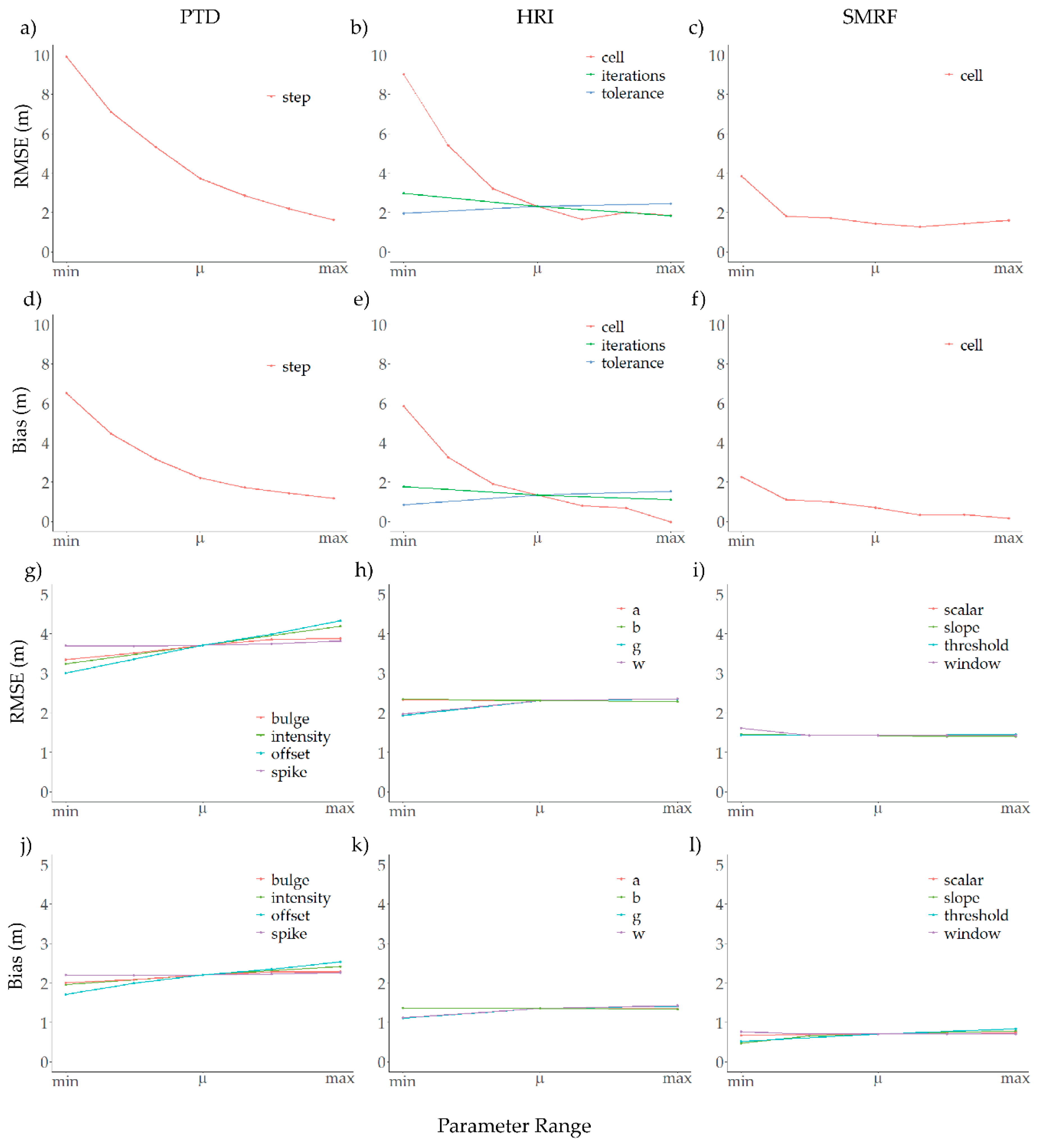
This study examined the achievable terrain-modeling accuracy of a low-cost UAS DAP data acquisition. Optimal parameters of three ground classification algorithms, designed for ALS point clouds, were determined using a sensitivity analysis and the variation in terrain-modeling accuracy was analyzed across local terrain slope and forest cover conditions.

Optimal parameter values for each method differed from the default algorithm values indicating that forested environments, in particular, the combined ICH and SBS BEC zones, require a unique set of parameter values to produce the most accurate DAP-DEM possible. The step, cell and cell parameters of the PTD, HRI and SMRF methods respectively had the greatest influence on DEM RMSE as for they specify the two-dimensional footprint of the initial search for ground points. Given the many ground classification algorithms that employ this fundamental step [53,58,59,60,61,63], the agreement between optimal step, cell and cell values of ~20 m indicate an initial search resolution likely appropriate for conifer stands of the ICH and SBS BEC zones.

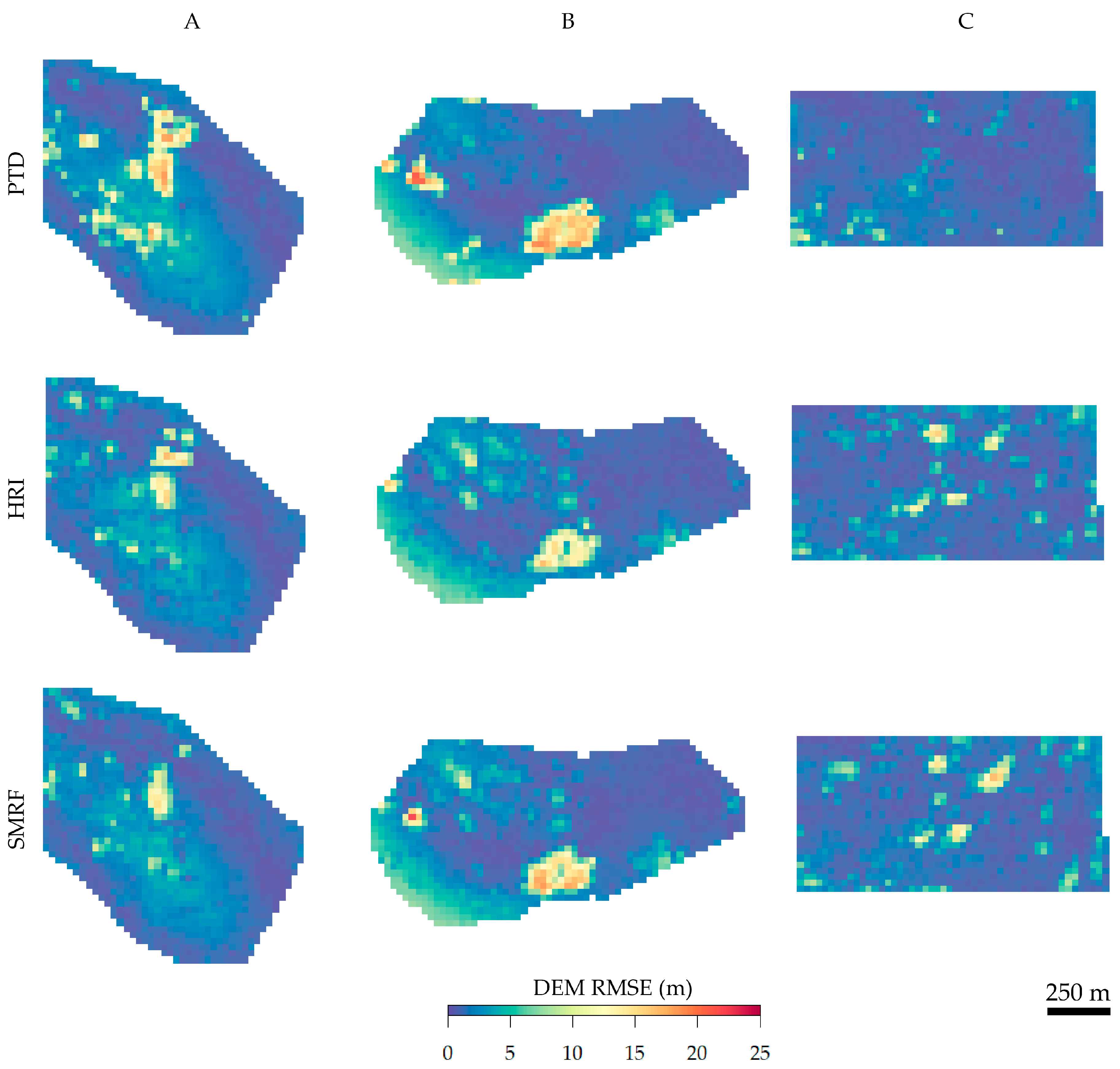
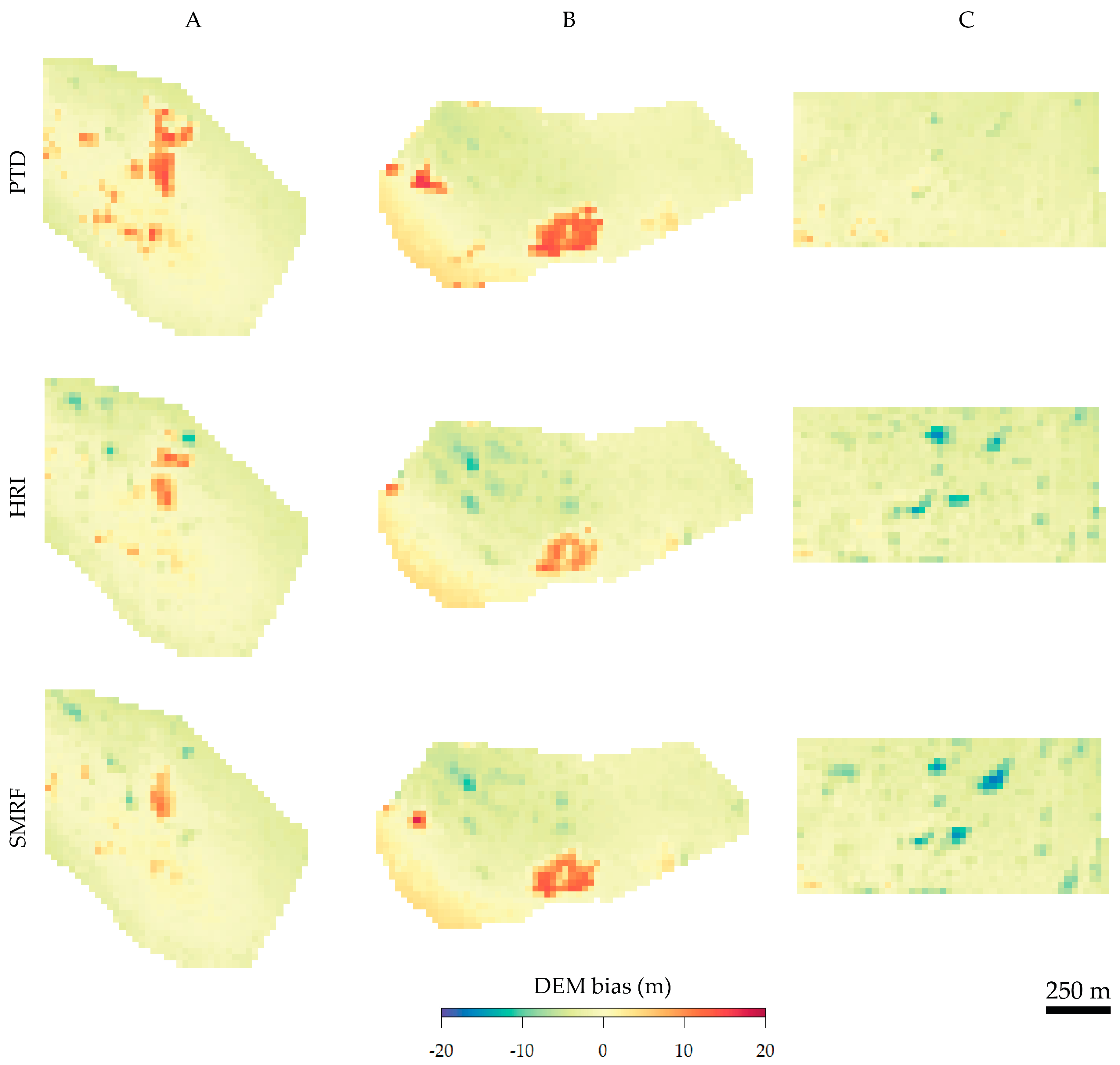
Following the sensitivity analysis, errors of the DAP-DEMs generated employing optimal parameters were compared to stratified classes of terrain slope and canopy cover derived from ALS point clouds. The relative importance of canopy cover was found to be approximately three times that of terrain slope when using optimal parameters of the best performing PTD classification method. We found that 57% of the terrain was modeled with an RMSE < 1.5 m. With this, assuming a mean tree height of 15 m, DEM error may contribute an error of 10% or less. Similar to this study’s findings, Iizuka et al. [30] generated terrain models within a forested environment from a UAS DAP point cloud and found normalized tree heights to be estimated with a minimum RMSE of 1.712 m. Similarly, Guerra-Hernández et al. [47] estimated tree heights with an RMSE of 1.82 m using a UAS DAP point cloud normalized by an ALS DEM. As another comparison, Goodbody et al. [29] were able to produce DAP derived ground models within low cover deciduous forests where the mean error reported was 0.01 m with a standard deviation of 0.14 m. While the results show a significant portion of the terrain was modeled adequately, large errors (>4 m) persist in areas of high canopy cover >80% where DAP was unable to register ground in areas larger than the defined initial search extent of the ground classification algorithms. In these areas, the algorithm misclassifies some canopy points as ground leading to a large over estimation in terrain elevation. Similar to results from this study, Guerra-Hernández et al. [47] report terrain height overestimation of >±2.0 m in areas of where slope was >20% and canopy cover >60%. Nevertheless, this study finds that there is potential for operationally acceptable DAP-DEM derivation where mean canopy cover is lower than around 70%.

Of the DAP acquisition parameters, flying altitude was restricted by local regulations to 122 m AGL while flight speed was restricted by the speed at which images are written to disk (5 Mb/s) and the desired image capture interval. As result of these restrictions, we were able to capture ~100 ha per day of flight. In comparison to a flat study site, terrain following over the mountainous terrain of the AFRF required additional power to climb and descend reducing the time of each flight. Up to eight readily charged batteries and subsequent takeoffs and landings were necessary in order to replace the battery.

This study assumes the canopy cover and terrain slope derived from ALS acquired in 2008 are adequate descriptions for analysis with DAP data acquired in 2017. We acknowledge that some degree of change to forest structure between the acquisitions is inevitable, and that a smaller temporal gap may have enhanced the relationship between canopy cover and the RMSE. In addition, the precision of GPS point measurement is known to be reduced within coniferous forests [72,73,74]. Therefore the error of GCP locations in complex forested terrain, such as in this region, likely reduced the agreement between DAP-DEMs and ALS points and therefore inflated RMSE. Tomaštík et al. [75] tested of a range of GCP configurations using a total station in three ~1 ha plots situated in flat, open canopy forests and report a mean vertical RMSE of ~0.1 m. Similarly, Jensen and Mathews [35] used eight GCP over ~15 ha where the landscape transitioned from savannah to closed canopy woodlands and found a mean estimated error of <0.15 m. Given these comparisons, future analyses involving the fusion of UAS DAP and ancillary spatial data over dense conifer forests requires a more precise direct or indirect georeferencing method for DAP point clouds. One possible solution is to deploy a more extensive GCP network using sub-centimeter precision differential GPS elevations collected from a total station such as done in [76]; however, defining and mapping the forest floor is challenging and the associated cost of such equipment is high. Another viable solution is the inclusion of higher precision GPS equipment onboard UASs, however this may erode the low-cost advantage of the UAS DAP approach. A third potential solution is the co-registration of the DAP point cloud with an independent, precisely georeferenced spatial dataset such as an ALS point cloud or an accurate road network layer with a high degree of spatial detail and coverage.

The range of forest conditions found within the chosen AFRF study area are typical of British Columbia’s ICH and SBS BEC zones, which account for 17% of British Columbia’s total land mass [77]. As previously mentioned the AFRF study areas were disturbed by wildfire in the months prior to image acquisition, potentially reducing over story foliage and therefore ground occlusion, providing the opportunity for a case study unique to stands disturbed by wildfire. Given recent catastrophic forest disturbances from the mountain pine beetle and wildfire across British Columbia, there is a demand from forest managers for the timely collection of structural information. For the many forest related natural resource management agencies around the province, the relatively low cost of UAS deployment compared to ALS opens new possibilities for such data collection. This study provides insight into the feasibility of UAS-DAP derived ground modeling in boreal and temperate forest biomes, which respectively account for 24.2% and 21.8% of global forests [78].

5. Conclusions

This study demonstrates the current capacity of typical low-cost UAS-DAP ground modeling results within the interior forests of central British Columbia. We found that DEMs derived from UAS DAP point clouds using existing ALS ground classification algorithms are comparable to ALS derived DEMs in a limited capacity largely due to the lack of ground points registered using DAP under dense forest canopies. Of the ground classification methods tested, PTD was able to model terrain accurately over a significantly larger area than HRI and SMRF methods. We confirm the expectation that DAP-DEM error is largely influenced by a combination of terrain slope and canopy cover and that canopy cover is more influential on error than terrain slope.

References

1. Korpela, I. Individual Tree Measurements by Means of Digital Aerial Photogrammetry; Silva Fennica: Helsinki, Finland, 2004; ISBN 0037-5330. [Google Scholar]
2. Takahashi, T.; Yamamoto, K.; Senda, Y.; Tsuzuku, M. Estimating individual tree heights of sugi (Cryptomeria japonica D. Don) plantations in mountainous areas using small-footprint airborne LiDAR. J. Res. 2005, 10, 135–142. [Google Scholar] [CrossRef]
3. Wang, Y.; Weinacker, H.; Koch, B. A Lidar Point Cloud Based Procedure for Vertical Canopy Structure Analysis And 3D Single Tree Modelling in Forest. Sensors 2008, 8, 3938–3951. [Google Scholar] [CrossRef] [PubMed]
4. Mohan, M.; Silva, C.; Klauberg, C.; Jat, P.; Catts, G.; Cardil, A.; Hudak, A.; Dia, M. Individual Tree Detection from Unmanned Aerial Vehicle (UAV) Derived Canopy Height Model in an Open Canopy Mixed Conifer Forest. Forests 2017, 8, 340. [Google Scholar] [CrossRef]
5. Gatziolis, D.; Lienard, J.F.; Vogs, A.; Strigul, N.S. 3D Tree Dimensionality Assessment Using Photogrammetry and Small Unmanned Aerial Vehicles. PLoS ONE 2015, 10, e0137765. [Google Scholar] [CrossRef] [PubMed]
6. White, J.C.; Wulder, M.A.; Varhola, A.; Vastaranta, M.; Coops, N.C.; Cook, B.D.; Pitt, D.; Woods, M. A best practices guide for generating forest inventory attributes from airborne laser scanning data using an area-based approach. For. Chron. 2013, 89, 722–723. [Google Scholar] [CrossRef] [Green Version]
7. Corona, P.; Fattorini, L. Area-based lidar-assisted estimation of forest standing volume. Can. J. For. Res. 2008, 38, 2911–2916. [Google Scholar] [CrossRef] [Green Version]
8. Turner, W.; Spector, S.; Gardiner, N.; Fladeland, M.; Sterling, E.; Steininger, M. Remote sensing for biodiversity science and conservation. Trends Ecol. Evol. 2003, 18, 306–314. [Google Scholar] [CrossRef]
9. Vierling, K.T.; Vierling, L.A.; Gould, W.A.; Martinuzzi, S.; Clawges, R.M. Lidar: Shedding new light on habitat characterization and modeling. Front. Ecol. Environ. 2008, 6, 90–98. [Google Scholar] [CrossRef]
10. Clarke, R.; Moses, L.B. The regulation of civilian drones’ impacts on public safety. Comput. Law Secur. Rev. 2014, 30, 263–285. [Google Scholar] [CrossRef]
11. Saha, B.; Koshimoto, E.; Quach, C.C.; Hogge, E.F.; Strom, T.H.; Hill, B.L.; Vazquez, S.L.; Goebel, K. Battery health management system for electric UAVs. IEEE Aerosp. Conf. Proc. 2011, 1–9. [Google Scholar] [CrossRef]
12. Amilton, J.A.D.H. Drones: A Rising Market. Appl. Econ. 2009, 91, 1257–1258. [Google Scholar] [CrossRef]
13. Malaek, S.M.; Kosari, A.R. Novel minimum time trajectory planning in terrain following flights. IEEE Trans. Aerosp. Electron. Syst. 2007, 43, 2–12. [Google Scholar] [CrossRef]
14. Shi, Y.; Thomasson, J.A.; Murray, S.C.; Pugh, N.A.; Rooney, W.L.; Shafian, S. Unmanned Aerial Vehicles for High-Throughput Phenotyping and Agronomic Research. PLoS ONE 2016, 11, e0159781. [Google Scholar] [CrossRef] [PubMed]
15. Scaioni, M.; Barazzetti, L.; Brumana, R.; Cuca, B.; Fassi, F.; Prandi, F. RC-Heli and structure & motion techniques for the 3-D reconstruction of a Milan Dome spire. ISPRS Int. Arch. Photogramm. Remote Sens. Spat. Inf. Sci. 2009, 38, 8. [Google Scholar]
16. Turner, D.; Lucieer, A.; Watson, C. An automated technique for generating georectified mosaics from ultra-high resolution Unmanned Aerial Vehicle (UAV) imagery, based on Structure from Motion (SFM) point clouds. Remote Sens. 2012, 4, 1392–1410. [Google Scholar] [CrossRef]
17. Baltsavias, E.P. A comparison between photogrammetry and laser scanning. ISPRS J. Photogramm. Remote Sens. 1999, 54, 83–94. [Google Scholar] [CrossRef]
18. Means, J.; Acker, S.; Fitt, B.; Renslow, M.; Emerson, L.; Hendrix, C. Predicting forest stand characteristics with airborne scanning lidar. Photogramm. Eng. Remote Sens. 2000, 66, 1367–1371. [Google Scholar] [CrossRef]
19. Neitzel, F.; Klonowski, J. Mobile 3D mapping with a low-cost UAV system. Int. Arch. Photogramm. Remote Sens. Inf. Sci. 2011, 38, 1–6. [Google Scholar] [CrossRef]
20. Mancini, F.; Dubbini, M.; Gattelli, M.; Stecchi, F.; Fabbri, S.; Gabbianelli, G. Using Unmanned Aerial Vehicles (UAV) for High-Resolution Reconstruction of Topography: The Structure from Motion Approach on Coastal Environments. Remote Sens. 2013, 5, 6880–6898. [Google Scholar] [CrossRef] [Green Version]
21. Mathews, A.; Jensen, J.L.R. Visualizing and Quantifying Vineyard Canopy LAI Using an Unmanned Aerial Vehicle (UAV) Collected High Density Structure from Motion Point Cloud. Remote Sens. 2013, 5, 2164–2183. [Google Scholar] [CrossRef] [Green Version]
22. Wallace, L.; Lucieer, A.; Malenovský, Z.; Turner, D.; Vopěnka, P. Assessment of Forest Structure Using Two UAV Techniques: A Comparison of Airborne Laser Scanning and Structure from Motion (SfM) Point Clouds. Forests 2016, 7, 62. [Google Scholar] [CrossRef]
23. Westoby, M.J.; Brasington, J.; Glasser, N.F.; Hambrey, M.J.; Reynolds, J.M. “Structure-from-Motion” photogrammetry: A low-cost, effective tool for geoscience applications. Geomorphology 2012, 179, 300–314. [Google Scholar] [CrossRef]
24. Woodcock, W.E. Aerial Reconnaissance and Photogrammetry with Small Cameras. Photogramm. Eng. Remote Sens. 1976, 42, 503–511. [Google Scholar]
25. Helava, U.V. Digital correlation in photogrammetric instruments. Photogrammetria 1978, 34, 19–41. [Google Scholar] [CrossRef]
26. Lane, S.N.; James, T.D.; Crowell, M.D. Application of digital photogrammetry to complex topography for geomorphological research. Photogramm. Rec. 2000, 16, 793–821. [Google Scholar] [CrossRef]
27. Smith, M.W.; Carrivick, J.L.; Quincey, D.J. Structure from motion photogrammetry in physical geography. Prog. Phys. Geogr. 2015, 40, 247–275. [Google Scholar] [CrossRef] [Green Version]
28. Tompalski, P.; Coops, N.C.; Marshall, P.L.; White, J.C.; Wulder, M.A.; Bailey, T. Combining multi-date airborne laser scanning and digital aerial photogrammetric data for forest growth and yield modelling. Remote Sens. 2018, 10, 347. [Google Scholar] [CrossRef]
29. Goodbody, T.R.H.; Coops, N.C.; Hermosilla, T.; Tompalski, P.; Pelletier, G. Vegetation Phenology Driving Error Variation in Digital Aerial Photogrammetrically Derived Terrain Models. Remote Sens. 2018, 10, 1554. [Google Scholar] [CrossRef]
30. Iizuka, K.; Yonehara, T.; Itoh, M.; Kosugi, Y. Estimating Tree Height and Diameter at Breast Height (DBH) from Digital surface models and orthophotos obtained with an unmanned aerial system for a Japanese Cypress (Chamaecyparis obtusa) Forest. Remote Sens. 2018, 10, 13. [Google Scholar] [CrossRef]
31. Guerra-Hernández, J.; González-Ferreiro, E.; Monleón, V.; Faias, S.; Tomé, M.; Díaz-Varela, R. Use of Multi-Temporal UAV-Derived Imagery for Estimating Individual Tree Growth in Pinus pinea Stands. Forests 2017, 8, 300. [Google Scholar] [CrossRef]
32. Rahlf, J.; Breidenbach, J.; Solberg, S.; Naesset, E.; Astrup, R. Digital aerial photogrammetry can efficiently support large-area forest inventories in Norway. For. Int. J. For. Res. For. 2017, 90, 710–718. [Google Scholar] [CrossRef]
33. Goodbody, T.R.H.; Coops, N.C.; Tompalski, P.; Crawford, P.; Day, K.J.K. Updating residual stem volume estimates using ALS-and UAV-acquired stereo-photogrammetric point clouds Updating residual stem volume estimates using ALS-and UAV-acquired stereo-photogrammetric point clouds. Int. J. Remote Sens. 2016, 38, 2938–2953. [Google Scholar] [CrossRef]
34. Clapuyt, F.; Vanacker, V.; Van Oost, K. Reproducibility of UAV-based earth topography reconstructions based on Structure-from-Motion algorithms. Geomorphology 2016, 260, 4–15. [Google Scholar] [CrossRef]
35. Jensen, J.L.R.; Mathews, A.J. Assessment of image-based point cloud products to generate a bare earth surface and estimate canopy heights in a woodland ecosystem. Remote Sens. 2016, 8, 50. [Google Scholar] [CrossRef]
36. Ota, T.; Ogawa, M.; Shimizu, K.; Kajisa, T.; Mizoue, N.; Yoshida, S.; Takao, G.; Hirata, Y.; Furuya, N.; Sano, T.; et al. Aboveground biomass estimation using structure from motion approach with aerial photographs in a seasonal tropical forest. Forests 2015, 6, 3882–3898. [Google Scholar] [CrossRef]
37. Lucieer, A.; de Jong, S.M.; Turner, D. Mapping landslide displacements using Structure from Motion (SfM) and image correlation of multi-temporal UAV photography. Prog. Phys. Geogr. 2014, 38, 97–116. [Google Scholar] [CrossRef]
38. Fonstad, M.A.; Dietrich, J.T.; Courville, B.C.; Jensen, J.L.; Carbonneau, P.E. Topographic structure from motion: A new development in photogrammetric measurement. Earth Surf. Process. Landf. 2013, 38, 421–430. [Google Scholar] [CrossRef]
39. Harwin, S.; Lucieer, A. Assessing the accuracy of georeferenced point clouds produced via multi-view stereopsis from Unmanned Aerial Vehicle (UAV) imagery. Remote Sens. 2012, 4, 1573–1599. [Google Scholar] [CrossRef]
40. Niethammer, U.; James, M.R.; Rothmund, S.; Travelletti, J.; Joswig, M. UAV-based remote sensing of the Super-Sauze landslide: Evaluation and results. Eng. Geol. 2012, 128, 2–11. [Google Scholar] [CrossRef]
41. St-Onge, B.; Vega, C.; Fournier, R.A.; Hu, Y. Mapping canopy height using a combination of digital stereo-photogrammetry and lidar. Int. J. Remote Sens. 2008, 29, 3343–3364. [Google Scholar] [CrossRef]
42. Korpela, I.; Anttila, P. Appraisal of the Mean Height of Trees by Means of Image Matching of Digitised Aerial Photographs. Photogramm. J. Finl. 2004, 19, 23–36. [Google Scholar]
43. Meng, X.; Currit, N.; Zhao, K. Ground Filtering Algorithms for Airborne LiDAR Data: A Review of Critical Issues. Remote Sens. 2010, 2, 833–860. [Google Scholar] [CrossRef] [Green Version]
44. Yan, L.; Liu, H.; Tan, J.; Li, Z.; Chen, C. A Multi-Constraint Combined Method for Ground Surface Point Filtering from Mobile LiDAR Point Clouds. Remote Sens. 2017, 9, 958. [Google Scholar] [CrossRef]
45. Barnard, S.T.; Fischler, M.A. Computational Stereo. ACM Comput. Surv. (CSUR) 1982, 14, 553–572. [Google Scholar] [CrossRef]
46. Kachamba, D.J.; Ørka, H.O.; Næsset, E.; Eid, T.; Gobakken, T. Influence of plot size on efficiency of biomass estimates in inventories of dry tropical forests assisted by photogrammetric data from an unmanned aircraft system. Remote Sens. 2017, 9, 610. [Google Scholar] [CrossRef]
47. Guerra-Hernández, J.; Cosenza, D.N.; Carlos, L.; Rodriguez, E.; Silva, M.; Tomé, M.; Díaz-Varela, R.A.; González-Ferreiro, E.; González, E.; Carlos Estraviz Rodriguez, L. Eucalyptus plantations. Int. J. Remote Sens. 2018, 39, 5211–5235. [Google Scholar] [CrossRef]
48. Day, K. History of the UBC Alex Fraser Research Forest (1987–2007)—Excerpts from Management and Working Plan # 3; University of British Columbia Alex Fraser Research Forest: Williams Lake, BC, Canada, 2007; Available online: http://afrf-forestry.sites.olt.ubc.ca/files/2012/03/MWP3WebQuality.pdf (accessed on 12 November 2018).
49. Klinka, K. Site Identification Tools, Field Site Maps, and Polygon Summaries for the UBC Alex Fraser Research Forest; UBC Alex Fraser Research Forest: Williams Lake, BC, Canada, 2004. [Google Scholar]
50. Soverel, N.O.; Perrakis, D.D.B.; Coops, N.C. Estimating burn severity from Landsat dNBR and RdNBR indices across western Canada. Remote Sens. Environ. 2010, 114, 1896–1909. [Google Scholar] [CrossRef]
51. Pix4Dmapper Pro Version 4.1. Available online: https://www.pix4d.com/ (accessed on 10 Decemeber 2018).
52. Coops, N.C.; Duffe, J.; Koot, C. Assessing the utility of lidar remote sensing technology to identify mule deer winter habitat. Can. J. Remote Sens. 2010, 36, 81–88. [Google Scholar] [CrossRef]
53. Zhang, W.; Qi, J.; Wan, P.; Wang, H.; Xie, D.; Wang, X.; Yan, G. An easy-to-use airborne LiDAR data filtering method based on cloth simulation. Remote Sens. 2016, 8, 501. [Google Scholar] [CrossRef]
54. Asghar, U. Landslide Mapping from Analysis of UAV-SFM Point Clouds. Ph.D. Thesis, University of British Columbia, Vancouver, BC, Canada, 2017. [Google Scholar]
55. Jat, P.; Serre, M.L. Bayesian Maximum Entropy space/time estimation of surface water chloride in Maryland using river distances. Environ. Pollut. 2016, 219, 1148–1155. [Google Scholar] [CrossRef]
56. Jat, P.; Serre, M.L. A novel geostatistical approach combining Euclidean and gradual-flow covariance models to estimate fecal coliform along the Haw and Deep rivers in North Carolina. Stoch. Environ. Res. Risk Assess. 2018, 32. [Google Scholar] [CrossRef]
57. Sithole, G.; Vosselman, G. Experimental comparison of filter algorithms for bare-Earth extraction from airborne laser scanning point clouds. ISPRS J. Photogramm. Remote Sens. 2004, 59, 85–101. [Google Scholar] [CrossRef]
58. Axelsson, P. Processing of laser scanner data—Algorithms and applications. ISPRS J. Photogramm. Remote Sens. 1999, 54, 138–147. [Google Scholar] [CrossRef]
59. Axelsson, P. DEM Generation from Laser Scanner Data Using adaptive TIN Models. Int. Arch. Photogramm. Remote Sens. 2000, 33, 110–117. [Google Scholar] [CrossRef]
60. Kraus, K.; Pfeifer, N. Determination of terrain models in wooded areas with airborne laser scanner data. ISPRS J. Photogramm. Remote Sens. 1998, 53, 193–203. [Google Scholar] [CrossRef]
61. Pingel, T.J.; Clarke, K.C.; Mcbride, W.A. An improved simple morphological filter for the terrain classification of airborne LIDAR data. ISPRS J. Photogramm. Remote Sens. 2013, 77, 21–30. [Google Scholar] [CrossRef]
62. Kilian, J.; Haala, N.; Markus, E. Capture and evaluation of airborne laser scanner data. Int. Arch. Photogramm. Remote Sens. 1996, 31, 383–388. [Google Scholar]
63. Zhang, K.; Chen, S.C.; Whitman, D.; Shyu, M.L.; Yan, J.; Zhang, C. A progressive morphological filter for removing nonground measurements from airborne LIDAR data. IEEE Trans. Geosci. Remote Sens. 2003, 41, 872–882. [Google Scholar] [CrossRef] [Green Version]
64. Zhang, J.; Lin, X. Filtering airborne LiDAR data by embedding smoothness-constrained segmentation in progressive TIN densification. ISPRS J. Photogramm. Remote Sens. 2013, 81, 44–59. [Google Scholar] [CrossRef]
65. Montealegre, A.L.; Lamelas, M.T.; De La Riva, J. A Comparison of Open—Source LiDAR Filtering Algorithms in a Mediterranean Forest Environment. IEEE J. Sel. Top. Appl. Earth Obs. Remote Sens. 2015, 8, 4072–4085. [Google Scholar] [CrossRef]
66. Isenburg, M.; Liu, Y.; Shewchuk, J.; Snoeyink, J.; Thirion, T. Generating Raster DEM from Mass Points via TIN Streaming. In International Conference on Geographic Information Science; Springer: Berlin/Heidelberg, Germany, 2006; pp. 186–198. [Google Scholar]
67. Hodgson, M.E.; Jensen, J.; Raber, G.; Tullis, J.; Davis, B.A.; Thompson, G.; Schuckman, K. An Evaluation of Lidar-derived Elevation and Terrain Slope in Leaf-off Conditions. Photogramm. Eng. Remote Sens. 2005, 71, 817–823. [Google Scholar] [CrossRef]
68. Korhonen, L.; Korpela, I.; Heiskanen, J.; Maltamo, M. Airborne discrete-return LIDAR data in the estimation of vertical canopy cover, angular canopy closure and leaf area index. Remote Sens. Environ. 2011, 115, 1065–1080. [Google Scholar] [CrossRef]
69. Nilsson, M. Estimation of tree heights and stand volume using an airborne lidar system. Remote Sens. Environ. 1996, 56, 1–7. [Google Scholar] [CrossRef]
70. Isenburg, M. LAStools. Available online: http://lastools.org (accessed on 10 August 2018).
71. Roussel, J.-R.; Auty, D. lidR: Airborne LiDAR Data Manipulation and Visualization for Forestry Applications. R Package Version 1.4.1. 2018. Available online: https://CRAN.R-project.org/package=lidR (accessed on 10 August 2018).
72. Deckert, C.; Bolstad, P. V Forest canopy, terrain, and distance effects on global positioning system point accuracy. Photogramm. Eng. Remote Sens. 1996, 62, 317–321. [Google Scholar]
73. Næsset, E. Point accuracy of combined pseudorange and carrier phase differential GPS under forest canopy. Can. J. For. Res. 1999, 29, 547–553. [Google Scholar] [CrossRef]
74. Reutebuch, S.E.; McGaughey, R.J.; Andersen, H.-E.; Carson, W.W. Accuracy of a high-resolution lidar terrain model under a conifer forest canopy. Can. J. Remote Sens. 2003, 29, 527–535. [Google Scholar] [CrossRef] [Green Version]
75. Tomaštík, J.; Mokroš, M.; Saloň, Š.; Chudý, F.; Tunák, D. Accuracy of Photogrammetric UAV-Based Point Clouds under Conditions of Partially-Open Forest Canopy. Forests 2017, 8, 151. [Google Scholar] [CrossRef]
76. Simpson, J.; Smith, T.; Wooster, M. Assessment of Errors Caused by Forest Vegetation Structure in Airborne LiDAR-Derived DTMs. Remote Sens. 2017, 9, 1101. [Google Scholar] [CrossRef]
77. British Columbia—Ministry of Forest, Lands, Natural Resource Operations and Rural Development. Biogeoclimatic Ecosystem Classification (BEC) Map; British Columbia—Ministry of Forest, Lands, Natural Resource Operations and Rural Development: Victoria, BC, Canada, 2018.
78. Crowther, T.W.; Glick, H.B.; Covey, K.R.; Bettigole, C.; Maynard, D.S.; Thomas, S.M.; Smith, J.R.; Hintler, G.; Duguid, M.C.; Amatulli, G.; et al. Mapping tree density at a global scale. Nature 2015, 525, 201–205. [Google Scholar] [CrossRef]
Figure 1. Schematic workflow of DAP point cloud generation, ground filter sensitivity analysis and DEM error assessment.
Remotesensing 11 00084 g001
Figure 2. UAV acquired orthomosaics (a) of study areas A, B and C (i, ii, and iii) respectively with overlaid GCP locations, study area northeast of Williams Lake, BC (b), an example photo of GCP (0.7 m × 0.7 m) situated on steep slope in study area A (c), and subcanopy image taken at the northwest corner of study area A (d). The coordinate system used throughout this study is X, Y: NAD83, UTM Zone 10 N; and Z: NADV 88.
Remotesensing 11 00084 g002
Figure 3. Distribution of area-based ALS derived terrain slope and canopy cover per study area A (a,d), B (b,e), and C (c,f) defined at 25 m × 25 m cell resolution.
Remotesensing 11 00084 g003
Figure 4. Spatial distribution of the 1 m × 1 m resolution ALS derived slope layer for areas A, B and C respectively (ac), and canopy cover (df) defined at 25 m × 25 m cell resolution.
Remotesensing 11 00084 g004
Figure 5. Sensitivity analysis results of ALS ground points vs. DAP DEM surface elevations using ground classification methods PTD (a,d,g,j); HRI (b,e,h,k); and SMRF (c,f,i,l). Varied parameter ranges are combined in a relative scale.
Remotesensing 11 00084 g005
Figure 6. Spatial distribution of the ALS vs. DAP-DEM RMSE averaged using 25 × 25 m cells for the three study areas and ground classification methods.
Remotesensing 11 00084 g006
Figure 7. Spatial distribution of the ALS vs. DAP-DEM bias averaged using 25 × 25 m cells for the three study areas and ground classification methods.
Remotesensing 11 00084 g007
Figure 8. DEM RMSE vs. stratified classes of terrain slope and canopy cover for the three study areas (A, B and C) and ground classification algorithms tested (PTD, HRI and SMRF) and their respective optimal parameterizations found in Section 3.1. The strata combining terrain slope class 6 and canopy cover class 1 was not represented in area B an is denoted by the white square.
Remotesensing 11 00084 g008