Determining Regional-Scale Groundwater Recharge with GRACE and GLDAS


1
Key Laboratory of Agricultural Soil and Water Engineering in Arid and Semiarid Areas, Ministry of Education, Northwest A&F University, Yangling 712100, China
2
Department of Soil Science, University of Saskatchewan, Saskatoon, SK S7N 5C8, Canada
*
Authors to whom correspondence should be addressed.
Remote Sens. 2019, 11(2), 154; https://0-doi-org.brum.beds.ac.uk/10.3390/rs11020154
Submission received: 10 November 2018
/
Revised: 9 January 2019
/
Accepted: 11 January 2019
/
Published: 15 January 2019
(This article belongs to the Special Issue GRACE Facing the Challenge of Extreme Spatial and Temporal Scales)
Abstract
:Groundwater recharge (GR) is a key component of regional and global water cycles and is a critical flux for water resource management. However, recharge estimates are difficult to obtain at regional scales due to the lack of an accurate measurement method. Here, we estimate GR using Gravity Recovery and Climate Experiment (GRACE) and Global Land Data Assimilation System (GLDAS) data. The regional-scale GR rate is calculated based on the groundwater storage fluctuation, which is, in turn, calculated from the difference between GRACE and root zone soil water storage from GLDAS data. We estimated GR in the Ordos Basin of the Chinese Loess Plateau from 2002 to 2012. There was no obvious long-term trend in GR, but the annual recharge varies greatly from 30.8 to 66.5 mm year−1, 42% of which can be explained by the variability in the annual precipitation. The average GR rate over the 11-year period from GRACE data was 48.3 mm year−1, which did not differ significantly from the long-term average recharge estimate of 39.9 mm year−1 from the environmental tracer methods and one-dimensional models. Moreover, the standard deviation of the 11-year average GR is 16.0 mm year−1, with a coefficient of variation (CV) of 33.1%, which is, in most cases, comparable to or smaller than estimates from other GR methods. The improved method could provide critically needed, regional-scale GR estimates for groundwater management and may eventually lead to a sustainable use of groundwater resources.
1. Introduction
Groundwater recharge is a key link between surface water and groundwater. The recharge water not only replenishes groundwater reservoirs, but also carries solutes from the upper strata, which could potentially contaminate groundwater. Thus, groundwater recharge influences both groundwater quality and quantity. Therefore, sustainable management of aquifers requires accurate estimates of GR [1,2].
GR has been estimated using a variety of techniques, including physical, chemical, isotopic, and modelling techniques [3,4,5]. Among these methods, the tritium (3H) peak concentration method and chloride mass balance method (CMB) have been widely used in arid and semiarid regions at the point scale [3,6,7]. The half-life of 3H is 12.5 years. Therefore, the concentrations currently account for 1/16 of that in the early 1960s. It was confirmed that the bomb test tritium peak was undetectable in many places around the globe [8,9]. Even if it may be detectable at some locations, the 3H introduced by thermonuclear tests can now be found either at great depths (>20 m) or even in the groundwater [10], which practically eliminates the method for estimating recharge using historical 3H from the portfolio of methods when the unsaturated zone is shallow [11]. The CMB method can be further divided into the unsaturated zone and the saturated zone CMB. The unsaturated zone CMB estimates long-term GR rates from the chloride (Cl) concentrations in the soil profile at the point scale [6,12]. The saturated zone CMB, however, estimates GR from the Cl concentrations in the groundwater, which is a result of long-term mixing of Cl from various recharge sources. Therefore, the recharge rates obtained by the saturated zone CMB are at intermediate scales, ranging from 1 m2 to 10,000 m2 [3]. However, the Cl input from precipitation at the surface must balance the Cl output (GR) below the root zone for the unsaturated zone CMB and the Cl input to groundwater for the saturated zone CMB. Unfortunately, any land use or climate change could significantly disturb the equilibrium, and once it is disturbed, to re-establish the equilibrium could take as long as years to decades for the unsaturated zone CMB and decades to hundreds of years for the saturated zone CMB. Consequently, the CMB methods are only applicable to cases where there has been no recent land use and climate change.
GR is known to be episodic, but only the long-term average of GR is reproduced by the above-mentioned tracer methods, giving no information about the temporal evolution of GR. Conversely, the groundwater table fluctuation method (WTF), taking advantage of the sharp water table rise in response to a given recharge event, estimates GR on a much short time scale, such as the recharge from a rainfall event. Therefore, WTF can be used to capture transient GR and is particularly suited for investigating the seasonality and episodicity of GR. However, rainfall infiltration fronts tend to disperse over a long distance [13], and thus, the sharp water table rise required by WTF may not occur or may display only seasonal water-level fluctuations in a deep aquifer or in aquifers overlain by fine-textured soils through which water moves slowly.
Moreover, these aforementioned methods can only estimate GR at small (unsaturated zone CMB) or intermediate scales (saturated zone CMB and WTF) [3,11,14]. Because small-scale GR rates possess strong spatial variability [4,7,15] and in many applications are sparsely measured, aggregation to regional scales remains difficult. Even if an average for a region can be obtained, temporal information is lost in the CMB methods [16,17,18,19]. To solve these problems, several efforts have been undertaken to estimate the GR at large scales, such as modelling and baseflow separation methods. For the baseflow separation method to estimate GR, pumpage, evapotranspiration, and underflow to deep aquifers may be significant and should be estimated independently. Unfortunately, these estimates are rarely available and are often based on many assumptions. The validity of these assumptions dictates the accuracy of the estimated recharge rates [3,20]. Similarly, the model estimates largely depend on the choice of parameterization [21,22,23,24], which often generates unsatisfactory flux estimates [25,26]. Therefore, an alternative method that can accurately estimate GR at large spatial scales but short time scales is critically needed.
The Gravity Recovery and Climate Experiment (GRACE) satellites, launched in 2002 by the National Aeronautics and Space Administration (NASA) and the German Aerospace Center, is no longer active as of 2018. The GRACE product is derived from two satellites flying in tandem (GRACE-1 and GRACE-2) and has the potential to meet these demands [27,28,29]. Previous studies have evaluated GRACE data with groundwater level monitoring data on seasonal or annual trend signals [30,31,32,33,34,35,36,37,38,39,40]. For example, Strassberg et al. [39] reported that the GRACE-derived seasonal groundwater storage anomaly (GWSA) in the High Plains of the USA agreed well with estimates based on groundwater level measurements. This was further corroborated by studies conducted in Jordan [41], India [30], and China [36,38,42]. Furthermore, the GRACE-derived monthly GWSAs on the Chinese Loess Plateau were highly correlated with in situ measured GWSA data [40]. Therefore, GRACE data have been the most successful in evaluating the groundwater depletion rates.
Recently, a few attempts have been made to estimate regional-scale GR rates using GRACE data [43,44,45]. All these approaches obtain groundwater storage anomaly (GWSA) by subtracting the unsaturated zone soil water storage anomaly (SWSA) obtained through GLDAS product, from the total water storage anomaly (TWSA) obtained from GRACE data. Then, the change in GWSA can be related to GR through two regional-scale water budget approaches:
- The average recharge within a time period equals to the sum of change of groundwater storage and groundwater discharge [44,45]; the average change of groundwater storage can be evaluated by the slope of the best-fitted linear equation to the measured GWSA as a function of time; and the groundwater discharge is the sum of natural discharge and total water withdrawn by pumping wells, which need to be estimated from other methods or information.
- The water storage fluctuation method [43] is used to estimate recharge from the change of groundwater storage, which is analogous to the well-known water table fluctuation (WTF). More specifically, the change in GWSA between the peak and trough over the time interval of interest gives net recharge [43].
To obtain total recharge though approach (1), one must know a priori groundwater discharge due to natural and anthropogenic reasons, which are rarely available at the regional-scale. Different from approach (1), the attraction of approach (2) is that the GR can be estimated without additional regional discharge information, but only gives net recharge, i.e., the increase in groundwater storage. The total recharge as the sum of net recharge and the recharge that balance the discharge, cannot be evaluated through approach (2). Therefore, the objectives of this paper are: (1) to extend the water storage fluctuation method of Henry et al. [43] to estimate total GR at regional-scale without the hard-to-obtain regional groundwater discharge data; (2) to evaluate the uncertainty of the estimated total GR rates at the regional scale; and (3) to compare the obtained total recharge with the recharge obtained from the environmental tracer methods and one-dimensional models. We tested the feasibility of this method for regional-scale GR estimation in the Ordos Basin of the Chinese Loess Plateau.
2. Materials and Methods
2.1. Study Area
The Chinese Loess Plateau is in the middle reach of the Yellow River basin in North China. It covers approximately 640,000 km2 (33°∼41°N, 100°∼114°E) (Figure 1). The Loess deposits represent aeolian dust from the deserts of the north and northwest lifted by the winter northwesterlies and deposited on the Loess Plateau. As a result, the soils are coarser in texture in the northwest and finer in the southeast [46]. The continuous deposition in the last 800,000 years has resulted in a deep unsaturated zone, ranging from 30 to 100 m [47].
The Loess Plateau is characterized by an arid and semiarid continental monsoon climate. Precipitation mainly occurs from June to September, bringing 60–70% of the annual total precipitation in the form of high-intensity rainstorms [48]. Because the distance to the vapor source increases from southeast to northwest, the long-term annual precipitation decreases from more than 800 mm year−1 in the southeast to less than 200 mm year−1 in the northwest (Figure 1). Consequently, the vegetation type changes from forest through forest-steppe to typical-steppe, desert-steppe, and then to steppe-desert zones from southeast to northwest [49].
We selected the Ordos Basin (280,000 km2) in the middle of the Loess Plateau as our study area because a large body of work has been conducted to estimate GR from environmental tracers (tritium, chloride) and models [17,50,51,52,53,54,55,56,57]. In addition, the Ordos Basin is one of the largest-scale groundwater basins in the world, and is composed of different interconnected aquifer systems, including the Cambrian-Ordovician Karst Aquifer System, Cretaceous Aquifer System, Carbonate-Jurassic Aquifer System and Quaternary Aquifer System [58]. Moreover, there has been little irrigation [52,54,55], and precipitation is the main source of GR [58].
2.2. Isolation of GWSA from TWSA
TWSA changes at monthly or longer timescales should be dominated by SWSA and GWSA changes in the Ordos Basin. This is because other components have a negligible effect on TWSA. First, the estimated maximum snow water equivalent from the GLDAS model is 7.2 × 10⁻³ mm, which is three orders of magnitude lower than the TWSA and SWSA. Second, the interannual variations in biomass were shown to be negligible [60]. Third, on the Loess Plateau, the reservoir water storage is generally no greater than 0.53 mm year−1 water equivalent based on the Yellow River Water Resources Bulletin (http://www.yellowriver.gov.cn/other/hhgb/) (accessed 18 November 2017) (Table S1). Because the largest reservoir is located at the edge of the Loess Plateau and away from the Ordos Basin, the reservoir effect will be even smaller. Fourth, only a small fraction of soil, with a mean of −0.44 mm year−1 in water equivalent, is transported out of the study area due to erosion (http://www.yellowriver.gov.cn/nishagonggao/) (accessed 18 November 2017) (Table S2). Therefore, the erosion on the Loess Plateau, although severe, has a negligible effect on the TWSA. Therefore, in this study, we assume that the anomalies of TWSA are primarily determined by the SWSA and GWSA.
TWSA can be derived conveniently from the GRACE data, which are available in two forms: spherical harmonics data and mass concentration (Mascon) solutions. Relative to the spherical harmonics data, the GRACE Mascon solutions from the Center for Space Research (CSR) (http://www.csr.utexas.edu/grace) (accessed 18 November 2017) have a reduced leakage from land to ocean [61,62]. Moreover, Mascon data do not require post-processing filtering and have less dependency on scale factors [62]. Therefore, the GRACE Mascon solutions are adopted in this study. In the Ordos Basin, there are 156 monthly TWSA measurements available between April 2002 and August 2016. Unfortunately, data are missing for 9 months between 2013 and 2015, making the recharge estimates unreliable. Thus, GRACE data from 2013 to 2016 were excluded for estimating GR. However, the data in this period still show the long-term trend of groundwater storage change, and thus the data were included in the groundwater storage depletion calculation.
In the Ordos Basin, there has been a large volume of work on soil water storage, but the measurements were not systematic enough in depth and frequency to obtain root zone soil water storage over the period of 2002 to 2016. Instead, we adopted a similar approach to others [30,36,38,41,42] by capitalizing on the GLDAS data and obtaining root zone SWSA with the four well-tested, large-scale hydrological models, Community Land Model (CLM), National Centers for Environmental Prediction/Oregon State University/Air Force/Hydrologic Research Lab model (NOAH), Mosaic and Variable Infiltration Capacity model (VIC) of GLDAS model from NASA [63]. GLDAS integrates satellite-based and ground-based data sets for parameterizing, forcing and constraining the hydrological models. The simulated results included soil water contents in the top 3.4, 2.0, 3.5 and 1.9 m of the soil column for CLM, NOAH, Mosaic and VIC, respectively [63]. GLDAS has been used in numerous studies to estimate unsaturated zone storage where in situ measurements are not feasible in many and diverse regions of the world [39,64,65,66,67,68].
Rainfall water infiltrating beyond the rooting depth can be considered GR. However, rooting depth varies with climate, soil and vegetation. Rooting depths are generally greater in semiarid regions than in humid regions [69,70,71]. In the Ordos Basin, the average rooting depth is approximately 2.0 m for annual cereal crops and grasses [72,73,74] and is greater for some perennial grasses and woody species [75,76,77,78]. For recharge estimates, the modelling depth should be greater than or equal to the rooting depth. The four GLDAS models satisfy this requirement, and thus, we used the four models to calculate SWSA. Although the four models have different root depths, as shown above, they all simulate soil water in the root zone. Therefore, we regard the mean SWSA of the four models as the root zone SWSA.
The GWSA is obtained by subtracting the average SWSA of the four GLDAS hydrologic models [63] from the GRACE TWSA anomalies:
However, unlike the monthly average outputs from GLDAS [79], GRACE has irregular sampling intervals. In addition, a few monthly values of the GRACE data are missing. In this case, we used the linear interpolation method to acquire the regular monthly GRACE data that would match the GLDAS data in time. When a GRACE measurement (TWS) is missing at a specific time t (e.g., 15 May 2002), but TWS1 and TWS2 are available at an earlier t1 and later t2 point in time (t1 < t < t2), then the missing measurement TWS is calculated by the following formula:
2.3. Estimation of Groundwater Recharge
The WTF method was developed in the 1920s for estimating recharge from groundwater table fluctuation and has since gained wide application [80,81,82,83,84,85,86,87]. Briefly, the GR rate can be calculated by multiplying the change in head over a specified time interval by the specific yield [13]:
where R is the GR (in mm year−1), h is the height of the water table (in mm), and Sy is the specific yield (in %). The primary advantage of the WTF method is that this method requires no assumptions on the mechanisms for water movement through the unsaturated zone; thus, it can be applied to a variety of recharge mechanisms, including direct recharge from precipitation or irrigation, indirect recharge from flood channels, or local recharge through preferential flow paths [13]. There are two different variations of the WTF method. An important distinction between the two implementations of the WTF is whether they consider correction for unrealized recession. Recessional processes (e.g., evaporation, discharge to springs) continue while recharge is causing the water table to rise [86]. When is equal to the difference between the peak of the rise and low point of the extrapolated antecedent recession curve at the time of the peak (extrapolation method), the WTF method produces the total recharge. When is the difference in heads between two points in time, the WTF method produces a value for net recharge (no extrapolation) [13].
In this study, we use the WTF method to estimate the total GR. An important distinction between GRACE data-based WTF and other WTF applications is how to define recharge episodes. A recharge episode is defined as a period during which the total recharge significantly exceeds its steady-state condition in response to a substantial water-input event [86]. In the saturated zone, WTF recognizes a recharge episode by water table fluctuation following a storm [13]. In a thick unsaturated zone, recharge is also episodic, particularly for recharge due to preferential flow and focused recharge. The episodic recharge event may be short in duration, relative to the measurement interval of GRACE, and can be randomly distributed over space. However, all recharges in an area add to soil water and groundwater, increasing the mass of the area, and the resulting mass increase from each episode accumulates with time and can be readily detected in the form of mass change in a subsequent GRACE measurement. For a footprint as large as what GRACE has, a wet season (summer in the Ordos Basin) consisting of a series of storm events results in a series of recharge episodes that accumulate over time, creating GRACE-measurable storage increases. This is analogous to tree growth measurements: tree growth has diurnal and seasonal variability; monthly measurements may not detect daily variability, but can capture the salient feature of the growth rates over the season. Therefore, the convolution of these recharge episodes may be considered a response to a large storm (convolution of rainfall events minus evapotranspiration) and can be detected by GRACE as the total storage increment. Consequently, a recharge episode appears from the trough of decline () and finishes at the peak of the rise () (Figure 2). Additionally, the recessions continue after , while recharge causes the GWSA rise. This part of the recession is called unrealized recession. To obtain recharge from the curve, one approach is to assume that unrealized recession is negligible, while the second approach estimates and corrects for it episode by episode, and the third approach quantifies the system behavior with a functional relationship between the water level and the decline rate [86]. Here, we adopt the second method by estimating and correcting for the unrealized recession on an episode-by-episode basis. The antecedent recession curve was obtained by linear fitting GWSA as a function of time during the seasonal recession from the peak in the previous year () to the trough of decline (), and then the obtained linear equation was extrapolated to the time of the peak Finally, we obtain the (), which is the GWSA extrapolated from the antecedent recession curve (solid line) at the time of the peak (). The dashed line from () to () is the unrealized recession (Figure 2).
Because , the GR rate may be calculated by the following formula:
where is the peak of the rise and is the GWSA extrapolated from the antecedent recession curve (dashed line) to the time of the peak. All terms are expressed as rates (e.g., mm year−1). Equation (4) accounts for discharge occurring between and ; thus, the obtained recharge is the sum of recharge that compensates for discharge occurring () and the recharge that causes the water storage increase () (Figure 2). However, if we replace with , we obtain the net recharge (), disregarding the recharge that balances the discharge between to , as is adopted by Henry et al. [43]. Therefore, our method improves Henry et al. [43]’s method by incorporating the additional recharge (RD in Figure 2) that occurs during recessions (red dotted line in Figure 2).
Our method and Henry et al. [43]’s method are based on the traditional, widely used water table fluctuation method (WTF), which takes the primary advantage of the WTF, without assuming the mechanisms of water flow in the unsaturated zone. Furthermore, the lateral recharge or discharge between two GRACE measurement grids needs to be known or may, in many cases, be negligible due to the large footprint. Thus, the lateral recharge events within the footprint does not affect the total recharge estimate within the footprint. Thus, it can be applied to a variety of recharge mechanisms including direct recharge from precipitation or irrigation, indirect recharge from flood channels, or local recharge through preferential flow paths and other complex recharge processes [13]. However, WTF-based methods, including our study and that of Henry et al. [43], do not account for the recharge during the recession [13,86]. We will discuss the uncertainty associated with neglecting this portion of recharge in Section 2.4.
2.4. Uncertainty in Estimated Recharge Rates
We further considered the uncertainty in GR derived from the GRACE data and the hydrological models. For random errors, the uncertainty in the obtained GR may be calculated from the error propagation law [88,89]:
where represents the standard deviation of a certain variable and represents the partial derivative of R with respect to a variable. is the standard deviation of predicted SL using the regression equation (Figure 2), n is the number of years, indicates the standard deviation of GR, i is the ith year, and is the standard deviation of n-year average GR.
The TWSA uncertainty estimation was based on the approach suggested by Landerer and Swenson [90] and Scanlon et al. [61]. First, we obtained the residuals by removing long-term trends and inter-annual, annual, and semi-annual amplitudes from TWSA. Then, the interannual signals were further removed by fitting a 13-month moving average to the residuals because they also contributed significantly to the TWSA in the Ordos Basin. The standard deviation of the residual approximates the measurement uncertainty, which is expressed by .
For SWSA, we do not have measurements of SWSA, as stated earlier. Instead, the uncertainty of SWSA, was obtained from the monthly standard deviation among the four hydrological models [27,31,33,36,39,67,88].
The uncertainties considered above are random errors. However, there may be underestimation or overestimation due to neglecting processes that affect GR, which is systematic error. For example, the recharge during recessions is neglected, thus introducing systematic error. We define and as the possible maximum and minimum mean annual recharge during recessions, respectively. The maximum and minimum are considered the upper limit and lower limit of the 95% confidence interval. Then, the standard deviation of the variable can be approximated by the following formula [91]:
is the standard deviation of neglecting mean GR during recessions.
The total error accounting for both systematic error and random error can be calculated as by Vasquez and Whiting [92]:
is the total error of n-year average GR. κ is the value used to define uncertainty intervals for the mean of large samples from a normal distribution For the 95% confidence, κ is approximately equal to 1.96 for a normally distributed variable.
CV is the coefficient of variation of n-year average GR. is the n-year average GR.
3. Results
3.1. GRACE-Derived Groundwater Storage Anomaly (GWSA) Variations
Figure 3a shows the temporal distribution of the monthly precipitation averaged over the Ordos Basin from 2002 to 2016. There is pronounced seasonality in the monthly precipitation, characterized by intense rainfall between June to September and infrequent, small monthly precipitation during the remainder of the year. The wet season (May to October) accounts for 85% of the total precipitation, while the dry season (November to April) accounts for 15% of the annual precipitation (Figure 3a). The average annual precipitation over the Ordos Basin varied from 346 to 585 mm year−1 from 2002 to 2016 (Table S3), which is consistent with the findings of Feng et al. [93] and Xie et al. [40].
Figure 3b shows the temporal distribution of TWSA and SWSA over the Ordos Basin from 2002 to 2016. The monthly TWSA varied from 126.4 mm in 2004 to −107.1 mm in 2016 (Table S3), showing a general declining trend with time. However, SWSA did not show a clear long-term trend, neither decreasing nor increasing with time. Moreover, both TWSA and SWSA showed a pronounced seasonal cycle, with peak values in autumn and low values in early summer (Figure 3b).
Figure 3c shows the monthly distribution of GWSA over the Ordos Basin from 2002 to 2016. Because GWSA = TWSA − SWSA, GWSA showed a similar decreasing trend as TWSA, with a reduction of 6.0 mm year−1. Seasonality in GWSA is still apparent but much weaker than that of TWSA (Figure 3b,c). TWSA, SWSA, and GWSA peaked, on average, on 1 October, 12 September, and 3 February in the following year, respectively (Table S4). The month of maximum TWSA and SWSA agrees with the occurrence of major precipitation events in the Ordos Basin during the wet season (May to October). There was barely any delay in response to precipitation in TWSA and SWSA. However, there was a nearly four-month lag in GWSA. The recession of GWSA starts, on average, in March and ends in August (Table S4). Because of the four-month delay, the recession period corresponded to the precipitation that occurred in dry seasons (from November to April). Similarly, the rising limb of GWSA corresponded to the precipitation that occurred during the wet season (from May to October).
3.2. Comparison of GRACE-Derived Groundwater Recharge with Estimates from Other Methods
There was a recharge season in each year from 2002 to 2012 (Figure 3c), and a linear equation was fitted to each of the recession curves according to Figure 2. The number of measurements in each recession curve was 4 to 8, with an average of 6.5. The coefficient of determination R2 varied from 0.36 to 0.89, with an average of 0.63 (Table 1; p < 0.05), indicating the goodness of the fit. The 11-year average GR was 48.3 ± 12.5 mm year−1 over the Ordos Basin from 2002 to 2012. The annual GR rates varied from 30.8 to 66.5 mm year−1, indicating that the interannual GR varied greatly. However, there was no obvious long-term trend, either decreasing or increasing, in GR from 2002 to 2012.
We then compared estimates using our method, the method of Henry et al. [43], and the environmental tracer method (Figure 4). The GR calculated using Henry et al. [43]’s method varies from 9.6 to 50.8 mm year−1 (Table S5), with an average of 28.3 ± 13.8 mm year−1 for the 11 years. We also summarized GR estimates from the literature using environmental tracers and modelling in the region (in Table S6 and Figure 4). These estimates were strongly variable, ranging from 0.11 to 110 mm year−1 at different times and locations in the Ordos Basin, with an average of 39.9 ± 26.5 mm year−1. Therefore, the obtained average GR rate from GRACE data is 20 mm year−1 larger than that from the Henry et al. [43]’s method (p < 0.05). It is approximately 8 mm year−1 larger than that from the point-scale environmental tracer method, but the difference is not significantly different from 0 (p > 0.05).
3.3. Evaluation of the Uncertainty of the Estimated Total Groundwater Recharge Rates at Regional Scale
Table 2 lists the different error components in the uncertainty estimates based on Section 2.4. The obtained is 14.9 mm month−1 in the Ordos Basin, which is similar to the standard deviation of 13.5 mm month−1 in the Yellow River basin [61]. For random errors, the standard deviations varied from 18.1 to 36.6 mm year−1 for estimated annual GR (Equations (5) to (7)) but decreased to 7.7 mm year−1 for the 11-year average GR (Equation (8)).
As illustrated above, our method cannot account for GR in dry seasons. Fortunately, there is substantially smaller precipitation and larger evaporation-to-precipitation ratio in dry seasons than in wet season in the Ordos Basin [35,95]. In addition, because of that, the ratio of recharge to precipitation has been shown to be substantially smaller in dry seasons than in wet seasons in most climate zones [35,96,97]. Therefore, the recharge in dry seasons should be substantially smaller than that of wet seasons. However, in order to characterize the potential errors introduced by neglecting the dry season recharge, we assumed the worst-case scenarios: the ratio of recharge to precipitation in dry seasons is equal to that in wet seasons. In this case, since dry season precipitation was only 17.6% of that in the wet season (Figure 3a), the GR in the dry season was calculated as 8.5 mm year−1 (wet season recharge 48.3 mm × 17.6%). Therefore, the underestimation as a form of systematic error is equal to 2.1 mm year−1 (Equation (9)).
Combining the random errors and systematic errors, we calculated the total error and CV for the 11-year average GR from GRACE to be 16.0 mm year−1 and 33.1%, respectively (Equations (9) and (10)).
4. Discussion
4.1. GWSA Seasonality, Long-Term Change and Delay in Response to Precipitation
Seasonality in GWSA is still apparent but much weaker than that of TWSA (Figure 3b,c). The weakened GWSA may be attributed to root water uptake and evaporation that may have reduced precipitation-induced GWSA fluctuation. The exclusion of the “active” surface soil, where water storage fluctuates strongly due to frequent precipitation and evaporation, may also be a reason (Figure 3c). Similar seasonality in TWSA, SWSA and GWSA has also been observed in other regions around the world [39,98,99,100,101]. However, the seasonality in GWSA shown in the Ordos Basin is weaker than in the North China Plain [36], indicating a weaker control of climate (mainly precipitation) on GWSA. This may be due to the lower amount of precipitation in the Ordos Basin (472.1 mm on average) (Table S3) than on the North China Plain (589 mm on average) [36].
Precipitation was stable from 2002 to 2012, but increased drastically from 2013 to 2015. However, TWSA decreased with time, which is in line with previous reports in the same region [40]. Generally, precipitation should be the dominant factor of total water storage. In our case, however, the decreasing total water storage from 2002 to 2016 can be explained by groundwater depletion [40]. The average reduction of groundwater storage was 6.0 mm year−1 in the Ordos Basin from 2002 to 2016, which is consistent with the reported 6.5 mm year−1 from Xie et al. [40] in the Loess Plateau from 2005 to 2014. Xie et al. [40] compared GWSA variations derived from the spherical harmonics solutions, mascon solutions, and the Slepian localization of spherical harmonics solutions (Slepian solutions) of GRACE data, with those derived from 136 groundwater observation wells on the Loess Plateau. They showed that GWSA derived from GRACE matched well with that from groundwater observation wells. Although pumping for irrigation is not a widespread phenomenon in our study region, pumping of groundwater is essential for coal mining, industry and residential life. Furthermore, the precipitation and coal mining data were used by Xie et al. [40] for analyzing the causes of groundwater depletion, and their results showed that seasonal changes in groundwater storage are closely related to rainfall, but the groundwater depletion is mainly due to human activities (e.g., coal mining). Thus, Xie et al. [40] provided convincing evidence for the use of GRACE data to estimate GWSA in the Loess Plateau. Because the Ordos Basin is in the middle of the Loess Plateau and accounts for approximately one-half of the Loess Plateau (Figure 1), the conclusions regarding GRACE data validation and the reason for groundwater storage depletion in Xie et al. [40] are likely to be applicable to the Ordos Basin. Many studies have shown much larger long-term groundwater depletion. For example, there were GWSA depletion rates of 20.0, 22.0 and 20.4 mm year−1 in North India, North China and California’s Central Valley, respectively [31,33,102]. Unlike the Ordos Basin, those regions are under the influence of intensive pumping of groundwater for irrigation.
There was barely any delay in response to precipitation in TWSA and SWSA. However, there was a nearly four-month lag in GWSA. This time lag results from the time it takes for water to percolate from the soil surface to beyond the root zone. Water percolation can be a slow process, and may take months or years for the water from a given precipitation event to pass the root zone, and decades to thousands of years for the water to reach groundwater [51,54,103]. As shown in Figure 3a, 2003 was an extremely wet year, and the 2004, 2005, and 2006 were relatively dry years. As an example, at Changwu (southern portion of the Ordos Basin), the extreme rainfall event (313 mm) in August 2003 created a wetting front at a depth of 3.5 m by mid-October, 4 m by the end of November, and 5 m by the end of December in 2003 [104]. Meanwhile, for years without extreme precipitation, as indicated by the peaks of GWSA, soil water would mainly infiltrate to the bottom of the root zone early in the next year (February and March) (Table S4).
4.2. What Is the Difference between Estimates from Our Method and Other Methods?
The obtained average GR rate from GRACE data is not significantly different from the point-scale method (p > 0.05). Theoretically, the GRACE-derived GR should be larger than the average of the point-scale methods. This is because point-scale estimates, such as those from the CMB and 3H in the unsaturated zone, only represent piston flow recharge [53,54,105]; they do not account for preferential flow recharge. Preferential flow exists widely even in uniform soil [106]. Studies indicate that preferential flow recharge can be significant (38% to 87% of the recharge) in the Ordos Basin [17,107]. The contribution of the preferential flow could have been masked by the great variability in recharge estimates by the point-scale methods.
Our estimates are 20.0 mm year−1 greater than the mean net recharge obtained from the method of Henry et al. [43] (Figure 4). As we stated earlier, the total recharge is the sum of net recharge and the portion of the recharge that compensates for the discharge. However, the method of Henry et al. [43] only accounts for the net recharge that elevates the groundwater storage (RS in Figure 2). In contrast, our method not only considers the RS but also incorporates the recharge that compensates for the discharge (RD in Figure 2).
4.3. Precipitation Dominated the Interannual Variability in Groundwater Recharge between 2002 and 2012
There is no obvious long-term trend in GR from 2002 to 2012, but the annual recharge varies greatly (Figure 4). The interannual variability can partially be explained by the precipitation; there was a linear relationship between annual GR rates and annual precipitation, with an R2 of 0.2 (Figure 5). However, there was an obvious outlier (2004) in the linear relationship. Although the annual precipitation in 2004 (point A) was 15.7% lower than the long-term average annual rainfall, its annual GR rate was 66.5 mm year−1, which was much higher than the 11-year average. The residual effect from the previous year’s large precipitation may be the reason for the large GR in 2004, a low precipitation year.
Therefore, the GR in 2004 is excluded, and the R2 between GR and precipitation is as high as 0.42 (p < 0.05), which indicates that in the Ordos Basin, precipitation, in most cases, regulates GR. Many similar studies have also reported the dominance of GR by precipitation, with R2 > 0.7 [108,109,110,111]. The high R2 may be related to only temporal variability in our recharge data because we treated the Ordos Basin as one unit in the recharge calculation. However, when spatial variability is also included, the R2 can be much lower. For example, R2 < 0.3 was observed for recharge data synthesized from around the globe and from Australia [5,7]. This is because other explanatory variables, such as soil texture [112,113] and root depth [114], also contributed to the variability in the recharge.
4.4. Uncertainty of the Groundwater Recharge Estimate Based on GRACE Data Compared with Other Methods
In our uncertainty analysis, we assumed that recharge to precipitation ratios in the dry season were smaller than those in the wet season. Recharges in semiarid and arid regions mainly occur during periods of heavy rainfall, and thus exhibit a distinct seasonal pattern [96,97,115]. Groundwater is recharged by seasonally high rainfall in the Ordos Basin [35]. However, precipitation is much lower in the dry season [95]; thus, there is most likely a much smaller ratio of recharge to precipitation than in the wet season. Therefore, the obtained uncertainty estimate for the GR is likely to be conservative.
The total error and CV are 16.0 mm year−1 and 33.1%, respectively (Equations (10) and (11)) for the 11-year average GR. The CV values for the estimated water flux by CMB varied between 23 and 51% [17,52,116], whereas those based on historical tracer 3H were between 10% and 20% [10,117]. Thus, the uncertainty in the mean recharge estimate from GRACE data is acceptable, despite its large footprint.
4.5. Limitation
There was a consistent decreasing trend in GWSA. However, the average decreasing rate was 6.0 mm year−1 from 2002 to 2016, which is much smaller relative to the mean annual amplitude of GWSA (28.3 mm), and thus will likely not mask the seasonal rise in GWSA. In addition, the total GR rates were estimated from the difference between the peak GWSA and the extrapolated recession at the time of peak; thus, the declining trend does not affect the difference between and .
Ideally, GLDAS data should be validated at the regional scale. However, the validation requires long-term, extensive ground truthing, which has been done in only a few regions [118]. An alternative, as commonly practiced, is to use the average of multiple model outputs [30,33,36,39]. In our study, we took the average of four GLDAS models as a representative SWSA. The peak times between SWSA and TWSA matched well in most years, but differed in some years (on average, the difference was about 0.6 months). The “shifts” may reflect the poor timing of simulated soil-water storage changes as reported by several studies [43,119,120,121]. These may arise from the shallow simulation depth and the inaccurate vegetation and soil parameters for the GLDAS modelling region [43]. For more accurate estimation of groundwater recharge, some sort of calibration is desirable, but this is rarely done because of the scarcity of quality validation data. Despite the problem, Henry et al. [43] found the average annual net recharge using the GRACE data-based WTF was very similar to the recharge estimated from historical well observations [43]. This suggests the “shift” had a negligible influence on the estimated recharge, but a quantitative evaluation of the influence is a subject of future research.
The strong spatial variability in tracer-derived GR is quite typical worldwide [4]. Because the environmental tracer methods only yield long-term average GR rates at a point scale, we took the areal average of all the point-scale recharge estimates from the environmental tracer method. Although the timescales and spatial scales represented by the GRACE method and the environmental tracer methods are quite different, the average of many point-scale estimates distributed over the Ordos Basin using the environmental tracer method may be used to compare and constrain our GRACE estimates. This methodology is also used by many others [122,123,124]. In additional, WTF-GRACE (our method) and Henry et al. [43]’s method have the same data size and time scale (2002 to 2012). However, the point-scale methods (CMB, 3H peak method, one-dimensional model) estimate GR at different time scales: the CMB method calculates the GR of the past decades to thousands of years [116]; the 3H peak method estimates the average GR since the 1960s; the one-dimensional model outputs GR at any time scale, but the outputs are subject to high uncertainty due to lack of calibration data. Thus, it is very difficult to constrain the results of the three methods to the same number of years. However, there is little change in the long-term average precipitation on the Loess Plateau in the past 60 years [95]. Therefore, the long-term GR estimated from different methods may be comparable.
5. Conclusions
In this study, the improved WTF method was used to estimate regional-scale GR based on TWSA obtained from the GRACE satellites and SWSA inferred from GLDAS models. We tested this improved method in the Ordos Basin on the Chinese Loess Plateau from 2002 to 2012 and compared the estimated GR with that estimated by other widely used methods. The results show the following:
- Annual recharge varies from 30.8 to 66.5 mm year−1 between 2002 and 2012, 42% of which can be explained by annual precipitation variation. There was no obvious long-term trend in GR in the period. This suggests that precipitation dominates the interannual variability of GR in the Ordos Basin.
- The estimated mean recharge (48.3 mm year−1) was 20.0 mm year−1 greater than the mean net recharge obtained from the method of Henry et al. [43] and had no significant difference from the reported point-scale estimates.
- The estimated long-term recharge had a standard deviation of 16.0 mm year−1 and a CV of 33.1%, which was, in most cases, comparable to or smaller than that of other methods.
The results indicate that this improved method has acceptable accuracy. Different from previous methods, the improved method presented in this study can be used to estimate total GR at regional scales, which may also be applicable to regions with monsoon, continental and Mediterranean climates and where alternating wet-dry season cycles occur around the world. The improved method is projected to provide rational GR estimates at regional scales for preferable management and budgeting of groundwater resources.
Supplementary Materials
The following are available online at https://0-www-mdpi-com.brum.beds.ac.uk/2072-4292/11/2/154/s1, Table S1: The annual water storage variations in Wanjiazhai reservoirs on the Loess Plateau in 2003-2016, Data based on the Yellow River Water Resources Bulletin (http://www.yellowriver.gov.cn/other/hhgb/), Table S2: Annual sediment runoff records at Tongguan hydrological station with a drainage area 680,000 km2, Data based on the Yellow River Sediment Bulletin (http://www.yellowriver.gov.cn/nishagonggao/), Table S3: Statistics of precipitation, TWSA, SWSA, GWSA from 2002 to 2012, Table S4: The month of peak TWSA, SWSA, and GWSA in each year and the decline period of GWSA, Table S5: Groundwater recharge estimated via method of Henry et al. [43] and our method, Table S6: Groundwater recharge in the Ordos Basin estimated with different methods from different studies [47,50,51,52,53,54,55,57,105,125,126].
Author Contributions
B.S., Q.W. and H.H. conceived and designed the study; Q.W. collected the data and conducted the data analysis; Q.W. and B.S. wrote the manuscript; H.H. proposed many useful suggestions to improve its quality; B.S. and P.W. provided the financial support and rationalized the logic of the manuscript.
Funding
This work was partially funded by the Natural Science Foundation of China (41877017; 41630860), and Natural Science and Engineering Research Council of Canada (NSERC).
Acknowledgments
The authors thank the GRACE processing center (CSR) for allowing access to the GRACE data, Feng Wei for providing the source codes of GRACE data processing, and Zhong Yulong for the useful suggestions in data processing.
Conflicts of Interest
The authors declare no conflict of interest.
Abbreviations
| Cl | Chloride |
| CLM | Community Land Model |
| CMB | Chloride Mass Balance method |
| CSR | Center for Space Research |
| GLDAS | Global Land Data Assimilation System |
| GRACE | Gravity Recovery and Climate Experiment |
| GR | groundwater recharge |
| GWSA | Groundwater Storage Anomaly |
| 3H | Tritium |
| Mascon | Mass concentration |
| NASA | National Aeronautics and Space Administration |
| NOAH | National Centers for Environmental Prediction/Oregon State University/Air Force/Hydrologic Research Lab model |
| Slepian solutions | the Slepian localization of spherical harmonics solutions |
| SWSA | Soil Water Storage Anomaly |
| TWSA | Total Water Storage Anomaly |
| VIC | Variable Infiltration Capacity |
| WTF | Groundwater Table Fluctuation |
References
- Scanlon, B.R.; Faunt, C.C.; Longuevergne, L.; Reedy, R.C.; Alley, W.M.; McGuire, V.L.; McMahon, P.B. Groundwater depletion and sustainability of irrigation in the US High Plains and Central Valley. Proc. Natl. Acad. Sci. USA 2012, 109, 9320–9325. [Google Scholar] [CrossRef] [PubMed] [Green Version]
- Taylor, R.G.; Scanlon, B.; Döll, P.; Rodell, M.; van Beek, R.; Wada, Y.; Longuevergne, L.; Leblanc, M.; Famiglietti, J.S.; Edmunds, M.; et al. Ground water and climate change. Nat. Clim. Chang. 2013, 3, 322–329. [Google Scholar] [CrossRef]
- Scanlon, B.R.; Healy, R.W.; Cook, P.G. Choosing appropriate technique for quantifying groundwater recharge. Hydrogeol. J. 2002, 10, 18–39. [Google Scholar] [CrossRef]
- Scanlon, B.R.; Keese, K.E.; Flint, A.L.; Flint, L.E.; Gaye, C.B.; Edmunds, W.M.; Simmers, I. Global synthesis of groundwater recharge in semiarid and arid regions. Hydrol. Process. 2006, 20, 3335–3370. [Google Scholar] [CrossRef]
- Petheram, C.; Walker, G.; Grayson, R.; Thierfelder, T.; Zhang, L. Towards a framework for predicting impacts of land-use on recharge: 1. A review of recharge studies in Australia. Soil Res. 2002, 40, 397. [Google Scholar] [CrossRef]
- Allison, G.B.; Gee, G.W.; Tyler, S.W. Vadose-Zone Techniques for Estimating Groundwater Recharge in Arid and Semiarid Regions. Soil Sci. Soc. Am. J. 1994, 58, 6. [Google Scholar] [CrossRef]
- Kim, J.H.; Jackson, R.B. A Global Analysis of Groundwater Recharge for Vegetation, Climate, and Soils. Vadose Zone J. 2012, 11. [Google Scholar] [CrossRef] [Green Version]
- Butler, M.J.; Verhagen, B.T. Isotope Studies of a Thick Unsaturated Zone in a Semi-Arid Area of Southern Africa. Available online: https://inis.iaea.org/search/search.aspx?orig_q=RN:33003268 (accessed on 30 November 2018).
- Gaye, C.B.; Edmunds, W.M. Groundwater recharge estimation using chloride, stable isotopes and tritium profiles in the sands of northwestern Senegal. Environ. Geol. 1996, 27, 246–251. [Google Scholar] [CrossRef] [Green Version]
- Rangarajan, R.; Athavale, R.N. Annual replenishable ground water potential of India—An estimate based on injected tritium studies. J. Hydrol. 2000, 234, 38–53. [Google Scholar] [CrossRef]
- Koeniger, P.; Gaj, M.; Beyer, M.; Himmelsbach, T. Review on soil water isotope-based groundwater recharge estimations. Hydrol. Process. 2016, 30, 2817–2834. [Google Scholar] [CrossRef]
- Gee, G.W.; Hillel, D. Groundwater Recharge In Arid Regions—Review And Critique Of Estimation Methods. Hydrol. Process. 1988, 2, 255–266. [Google Scholar] [CrossRef]
- Healy, R.W.; Cook, P.G. Using groundwater levels to estimate recharge. Hydrogeol. J. 2002, 10, 91–109. [Google Scholar] [CrossRef]
- Sophocleous, M.A. Combining the soilwater balance and water-level fluctuation methods to estimate natural groundwater recharge: Practical aspects. J. Hydrol. 1991. [Google Scholar] [CrossRef]
- Wine, M.L.; Hendrickx, J.M.H.; Cadol, D.; Zou, C.B.; Ochsner, T.E. Deep drainage sensitivity to climate, edaphic factors, and woody encroachment, Oklahoma, USA. Hydrol. Process. 2015, 29, 3779–3789. [Google Scholar] [CrossRef]
- Custodio, E.; Jódar, J. Simple solutions for steady–state diffuse recharge evaluation in sloping homogeneous unconfined aquifers by means of atmospheric tracers. J. Hydrol. 2016, 540, 287–305. [Google Scholar] [CrossRef]
- Li, Z.; Chen, X.; Liu, W.; Si, B. Determination of groundwater recharge mechanism in the deep loessial unsaturated zone by environmental tracers. Sci. Total Environ. 2017, 586, 827–835. [Google Scholar] [CrossRef] [PubMed]
- Wood, W.W.; Sanford, W.E. Chemical and Isotopic Methods for Quantifying Ground-Water Recharge in a Regional, Semiarid Environment. Ground Water 1995, 33, 458–468. [Google Scholar] [CrossRef]
- Dyck, M.F.; Kachanoski, R.G.; de Jong, E. Long-term Movement of a Chloride Tracer under Transient, Semi-Arid Conditions. Soil Sci. Soc. Am. J. 2003, 67, 471. [Google Scholar] [CrossRef]
- Chemingui, A.; Sulis, M.; Paniconi, C. An assessment of recharge estimates from stream and well data and from a coupled surface-water/groundwater model for the des Anglais catchment, Quebec (Canada). Hydrogeol. J. 2015, 23, 1731–1743. [Google Scholar] [CrossRef]
- Andreasen, M.; Andreasen, L.A.; Jensen, K.H.; Sonnenborg, T.O.; Bircher, S. Estimation of Regional Groundwater Recharge Using Data from a Distributed Soil Moisture Network. Vadose Zone J. 2013, 12. [Google Scholar] [CrossRef]
- Assefa, K.A.; Woodbury, A.D. Transient, spatially varied groundwater recharge modeling. Water Resour. Res. 2013, 49, 4593–4606. [Google Scholar] [CrossRef] [Green Version]
- Cao, G.; Zheng, C.; Scanlon, B.R.; Liu, J.; Li, W. Use of flow modeling to assess sustainability of groundwater resources in the North China Plain. Water Resour. Res. 2013, 49, 159–175. [Google Scholar] [CrossRef] [Green Version]
- Carrera-Hernández, J.J.; Smerdon, B.D.; Mendoza, C.A. Estimating groundwater recharge through unsaturated flow modelling: Sensitivity to boundary conditions and vertical discretization. J. Hydrol. 2012, 452–453, 90–101. [Google Scholar] [CrossRef]
- Qi, W.; Zhang, C.; Fu, G.T.; Zhou, H.C. Global Land Data Assimilation System data assessment using a distributed biosphere hydrological model. J. Hydrol. 2015, 528, 652–667. [Google Scholar] [CrossRef]
- Robock, A.; Luo, L.F.; Wood, E.F.; Wen, F.H.; Mitchell, K.E.; Houser, P.R.; Schaake, J.C.; Lohmann, D.; Cosgrove, B.; Sheffield, J.; et al. Evaluation of the North American Land Data Assimilation System over the southern Great Plains during the warm season. J. Geophys. Res. 2003, 108, 8846. [Google Scholar] [CrossRef]
- Rodell, M.; Famiglietti, J.S. The potential for satellite-based monitoring of groundwater storage changes using GRACE: The High Plains aquifer, Central US. J. Hydrol. 2002, 263, 245–256. [Google Scholar] [CrossRef]
- Swenson, S.; Wahr, J. Methods for inferring regional surface-mass anomalies from Gravity Recovery and Climate Experiment (GRACE) measurements of time-variable gravity. J. Geophys. Res. Solid Earth 2002, 107, 2193. [Google Scholar] [CrossRef]
- Molina, J.L.; García Aróstegui, J.L.; Benavente, J.; Varela, C.; de la Hera, A.; López Geta, J.A. Aquifers overexploitation in SE Spain: A proposal for the integrated analysis of water management. Water Resour. Manag. 2009. [Google Scholar] [CrossRef]
- Bhanja, S.N.; Mukherjee, A.; Saha, D.; Velicogna, I.; Famiglietti, J.S. Validation of GRACE based groundwater storage anomaly using in-situ groundwater level measurements in India. J. Hydrol. 2016, 543, 729–738. [Google Scholar] [CrossRef]
- Famiglietti, J.S.; Lo, M.; Ho, S.L.; Bethune, J.; Anderson, K.J.; Syed, T.H.; Swenson, S.C.; de Linage, C.R.; Rodell, M. Satellites measure recent rates of groundwater depletion in California’s Central Valley. Geophys. Res. Lett. 2011, 38, L03403. [Google Scholar] [CrossRef]
- Frappart, F.; Papa, F.; Güntner, A.; Werth, S.; Santos da Silva, J.; Tomasella, J.; Seyler, F.; Prigent, C.; Rossow, W.B.; Calmant, S.; et al. Satellite-based estimates of groundwater storage variations in large drainage basins with extensive floodplains. Remote Sens. Environ. 2011, 115, 1588–1594. [Google Scholar] [CrossRef] [Green Version]
- Feng, W.; Zhong, M.; Lemoine, J.M.; Biancale, R.; Hsu, H.T.; Xia, J. Evaluation of groundwater depletion in North China using the Gravity Recovery and Climate Experiment (GRACE) data and ground-based measurements. Water Resour. Res. 2013, 49, 2110–2118. [Google Scholar] [CrossRef] [Green Version]
- Ramillien, G.; Frappart, F.; Cazenave, A.; Güntner, A. Time variations of land water storage from an inversion of 2 years of GRACE geoids. Earth Planet. Sci. Lett. 2005, 235, 283–301. [Google Scholar] [CrossRef] [Green Version]
- Huang, T.; Pang, Z.; Edmunds, W.M. Soil profile evolution following land-use change: Implications for groundwater quantity and quality. Hydrol. Process. 2013, 27, 1238–1252. [Google Scholar] [CrossRef]
- Huang, Z.; Pan, Y.; Gong, H.; Yeh, P.J.F.; Li, X.; Zhou, D.; Zhao, W. Subregional-scale groundwater depletion detected by GRACE for both shallow and deep aquifers in North China Plain. Geophys. Res. Lett. 2015, 42, 1791–1799. [Google Scholar] [CrossRef] [Green Version]
- Shamsudduha, M.; Taylor, R.G.; Longuevergne, L. Monitoring groundwater storage changes in the highly seasonal humid tropics: Validation of GRACE measurements in the Bengal Basin. Water Resour. Res. 2012, 48. [Google Scholar] [CrossRef] [Green Version]
- Shen, H.; Leblanc, M.; Tweed, S.; Liu, W. Groundwater depletion in the Hai River Basin, China, from in situ and GRACE observations. Hydrol. Sci. J. 2015, 60, 671–687. [Google Scholar] [CrossRef]
- Strassberg, G.; Scanlon, B.R.; Rodell, M. Comparison of seasonal terrestrial water storage variations from GRACE with groundwater-level measurements from the High Plains Aquifer (USA). Geophys. Res. Lett. 2007, 34, L14402. [Google Scholar] [CrossRef]
- Xie, X.; Xu, C.; Wen, Y.; Li, W. Monitoring Groundwater Storage Changes in the Loess Plateau Using GRACE Satellite Gravity Data, Hydrological Models and Coal Mining Data. Remote Sens. 2018, 10, 605. [Google Scholar] [CrossRef]
- Liesch, T.; Ohmer, M. Comparison of GRACE data and groundwater levels for the assessment of groundwater depletion in Jordan. Hydrogeol. J. 2016, 24, 1547–1563. [Google Scholar] [CrossRef]
- Yin, W.; Hu, L.; Jiao, J.J. Evaluation of Groundwater Storage Variations in Northern China Using GRACE Data. Geofluids 2017, 2017, 1–13. [Google Scholar] [CrossRef] [Green Version]
- Henry, C.M.; Allen, D.M.; Huang, J. Groundwater storage variability and annual recharge using well-hydrograph and GRACE satellite data. Hydrogeol. J. 2011, 19, 741–755. [Google Scholar] [CrossRef]
- Gonçalvès, J.; Petersen, J.; Deschamps, P.; Hamelin, B.; Baba-Sy, O. Quantifying the modern recharge of the “fossil” Sahara aquifers. Geophys. Res. Lett. 2013, 40, 2673–2678. [Google Scholar] [CrossRef] [Green Version]
- Ahmed, M.; Abdelmohsen, K. Quantifying Modern Recharge and Depletion Rates of the Nubian Aquifer in Egypt. Surv. Geophys. 2018, 39, 729–751. [Google Scholar] [CrossRef]
- Wang, Y.; Shao, M.; Zhu, Y.; Liu, Z. Impacts of land use and plant characteristics on dried soil layers in different climatic regions on the Loess Plateau of China. Agric. For. Meteorol. 2011, 151, 437–448. [Google Scholar] [CrossRef]
- Huang, T.; Yang, S.; Liu, J.; Li, Z. How much information can soil solute profiles reveal about groundwater recharge? Geosci. J. 2016, 20, 495–502. [Google Scholar] [CrossRef]
- Liang, W.; Bai, D.; Wang, F.; Fu, B.; Yan, J.; Wang, S.; Yang, Y.; Long, D.; Feng, M. Quantifying the impacts of climate change and ecological restoration on streamflow changes based on a Budyko hydrological model in China’s Loess Plateau. Water Resour. Res. 2015, 51, 6500–6519. [Google Scholar] [CrossRef]
- Shi, H.; Shao, M. Soil and water loss from the Loess Plateau in China. J. Arid Environ. 2000, 45, 9–20. [Google Scholar] [CrossRef]
- Chen, J.S.; Liu, X.Y.; Wang, C.Y.; Rao, W.B.; Tan, H.B.; Dong, H.Z.; Sun, X.X.; Wang, Y.S.; Su, Z.G. Isotopic constraints on the origin of groundwater in the Ordos Basin of northern China. Environ. Earth Sci. 2012, 66, 505–517. [Google Scholar] [CrossRef]
- Gates, J.B.; Scanlon, B.R.; Mu, X.; Zhang, L. Impacts of soil conservation on groundwater recharge in the semi-arid Loess Plateau, China. Hydrogeol. J. 2011, 19, 865–875. [Google Scholar] [CrossRef]
- Huang, T.; Pang, Z. Estimating groundwater recharge following land-use change using chloride mass balance of soil profiles: A case study at Guyuan and Xifeng in the Loess Plateau of China. Hydrogeol. J. 2011, 19, 177–186. [Google Scholar] [CrossRef]
- Huang, T.; Pang, Z.; Liu, J.; Ma, J.; Gates, J. Groundwater recharge mechanism in an integrated tableland of the Loess Plateau, northern China: Insights from environmental tracers. Hydrogeol. J. 2017, 25, 2049–2065. [Google Scholar] [CrossRef]
- Huang, T.M.; Pang, Z.H.; Liu, J.L.; Yin, L.H.; Edmunds, W.M. Groundwater recharge in an arid grassland as indicated by soil chloride profile and multiple tracers. Hydrol. Process. 2017, 31, 1047–1057. [Google Scholar] [CrossRef]
- Yin, L.H.; Hu, G.C.; Huang, J.T.; Wen, D.G.; Dong, J.Q.; Wang, X.Y.; Li, H.B. Groundwater-recharge estimation in the Ordos Plateau, China: Comparison of methods. Hydrogeol. J. 2011, 19, 1563–1575. [Google Scholar] [CrossRef]
- Turkeltaub, T.; Jia, X.; Zhu, Y.; Shao, M.-A.; Binley, A. Recharge and Nitrate Transport Through the Deep Vadose Zone of the Loess Plateau: A Regional-Scale Model Investigation. Water Resour. Res. 2018, 54, 4332–4346. [Google Scholar] [CrossRef]
- Li, H.; Si, B.; Jin, J.; Zhang, Z.; Wu, Q.; Wang, H. Estimating of Deep Drainage Rates on the Slope Land of Loess Plateau Based on the Use of Environment Tritium (In Chinese). J. Soil Water Conserv. 2013, 30, 91–95. [Google Scholar]
- Hou, G.C.; Liang, Y.P.; Su, X.S.; Zhao, Z.H.; Tao, Z.P.; Yin, L.H.; Yang, Y.C.; Wang, X.Y. Groundwater Systems and Resources in the Ordos Basin, China. Acta Geol. Sin. Ed. 2008, 82, 1061–1069. [Google Scholar]
- Simunek, J.; Van Genuchten, M.T.; Sejna, M. The HYDRUS-1D software package for simulating the one-dimensional movement of water, heat, and multiple solutes in variably-saturated media. Univ. Calif. Riverside Res. Rep. 2005, 3, 1–240. [Google Scholar]
- Rodell, M.; Chao, B.F.; Au, A.Y.; Kimball, J.S.; McDonald, K.C. Global biomass variation and its geodynamic effects: 1982-98. Earth Interact. 2005, 9. [Google Scholar] [CrossRef]
- Scanlon, B.R.; Zhang, Z.; Save, H.; Wiese, D.N.; Landerer, F.W.; Long, D.; Longuevergne, L.; Chen, J. Global evaluation of new GRACE mascon products for hydrologic applications. Water Resour. Res. 2016, 52, 9412–9429. [Google Scholar] [CrossRef] [Green Version]
- Save, H.; Bettadpur, S.; Tapley, B.D. High-resolution CSR GRACE RL05 mascons. J. Geophys. Res. Solid Earth 2016, 121, 7547–7569. [Google Scholar] [CrossRef]
- Rodell, M.; Houser, P.R.; Jambor, U.; Gottschalck, J.; Mitchell, K.; Meng, C.-J.; Arsenault, K.; Cosgrove, B.; Radakovich, J.; Bosilovich, M.; et al. The Global Land Data Assimilation System. Bull. Am. Meteorol. Soc. 2004, 85, 381–394. [Google Scholar] [CrossRef] [Green Version]
- Rodell, M.; Chen, J.; Kato, H.; Famiglietti, J.S.; Nigro, J.; Wilson, C.R. Estimating groundwater storage changes in the Mississippi River basin (USA) using GRACE. Hydrogeol. J. 2007, 15, 159–166. [Google Scholar] [CrossRef]
- Leblanc, M.J.; Tregoning, P.; Ramillien, G.; Tweed, S.O.; Fakes, A. Basin-scale, integrated observations of the early 21st century multiyear drought in Southeast Australia. Water Resour. Res. 2009, 45, 1–10. [Google Scholar] [CrossRef]
- Andersen, O.B.; Seneviratne, S.I.; Hinderer, J.; Viterbo, P. GRACE-derived terrestrial water storage depletion associated with the 2003 European heat wave. Geophys. Res. Lett. 2005, 32, L18405. [Google Scholar] [CrossRef]
- Rodell, M.; Velicogna, I.; Famiglietti, J.S. Satellite-based estimates of groundwater depletion in India. Nature 2009, 460, 999–1002. [Google Scholar] [CrossRef] [PubMed] [Green Version]
- Tiwari, V.M.; Wahr, J.; Swenson, S. Dwindling groundwater resources in northern India, from satellite gravity observations. Geophys. Res. Lett. 2009, 36, 1–5. [Google Scholar] [CrossRef]
- Schenk, H.J.; Jackson, R.B. The Global Biogeography of Roots. Ecol. Monogr. 2002, 72, 311. [Google Scholar] [CrossRef]
- Schenk, H.J.; Jackson, R.B. Rooting depths, lateral root spreads and below-ground/above-ground allometries of plants in water-limited ecosystems. J. Ecol. 2002, 90, 480–494. [Google Scholar] [CrossRef] [Green Version]
- Schenk, H.J.; Jackson, R.B. Mapping the global distribution of deep roots in relation to climate and soil characteristics. Geoderma 2005, 126, 129–140. [Google Scholar] [CrossRef]
- Kang, S.; Zhang, L.; Liang, Y.; Hu, X.; Cai, H.; Gu, B. Effects of limited irrigation on yield and water use efficiency of winter wheat in the Loess Plateau of China. Agric. Water Manag. 2002, 55, 203–216. [Google Scholar] [CrossRef]
- Yang, L.; Wei, W.; Chen, L.; Chen, W.; Wang, J. Response of temporal variation of soil moisture to vegetation restoration in semi-arid Loess Plateau, China. CATENA 2014, 115, 123–133. [Google Scholar] [CrossRef] [Green Version]
- Zhou, L.-M.; Li, F.-M.; Jin, S.-L.; Song, Y. How two ridges and the furrow mulched with plastic film affect soil water, soil temperature and yield of maize on the semiarid Loess Plateau of China. Field Crop. Res. 2009, 113, 41–47. [Google Scholar] [CrossRef]
- Ma, L.H.; Wu, P.t.; Wang, Y.k. Spatial distribution of roots in a dense jujube plantation in the semiarid hilly region of the Chinese Loess Plateau. Plant Soil 2012, 354, 57–68. [Google Scholar] [CrossRef]
- Wang, Y.; Shao, M.; Liu, Z.; Zhang, C. Characteristics of Dried Soil Layers Under Apple Orchards of Different Ages and Their Applications in Soil Water Managements on the Loess Plateau of China. Pedosphere 2015, 25, 546–554. [Google Scholar] [CrossRef]
- Wang, Z.; Liu, B.; Zhang, Y. Soil moisture of different vegetation types on the loess Plateau. J. Geogr. Sci. 2009, 19, 707–718. [Google Scholar] [CrossRef]
- Zhou, Z.; Shangguan, Z. Vertical distribution of fine roots in relation to soil factors in Pinus tabulaeformis Carr. forest of the Loess Plateau of China. Plant Soil 2007, 291, 119–129. [Google Scholar] [CrossRef]
- Rui, H.; Beaudoing, H. Readme document for global land data assimilation system version 2 (GLDAS-2) products. GES DISC 2011, 2011. [Google Scholar]
- Freeze, R.A. The Mechanism of Natural Ground-Water Recharge and Discharge: 1. One-dimensional, Vertical, Unsteady, Unsaturated Flow above a Recharging or Discharging Ground-Water Flow System. Water Resour. Res. 1969, 5, 153–171. [Google Scholar] [CrossRef]
- Gerhart, J.M. Ground-Water Recharge and Its Effects on Nitrate Concentration Beneath a Manured Field Site in Pennsylvania. Groundwater 1986, 24, 483–489. [Google Scholar] [CrossRef]
- Calder, I.R.; Hall, R.L.; Prasanna, K.T. Hydrological impact of Eucalyptus plantation in India. J. Hydrol. 1993, 150, 635–648. [Google Scholar] [CrossRef]
- Heppner, C.S.; Nimmo, J.R. A Computer Program for Predicting Recharge with a Master Recession Curve. Available online: https://wwwrcamnl.wr.usgs.gov/uzf/abs_pubs/papers/SIR5172.pdf (accessed on 30 November 2018).
- Maréchal, J.C.; Dewandel, B.; Ahmed, S.; Galeazzi, L.; Zaidi, F.K. Combined estimation of specific yield and natural recharge in a semi-arid groundwater basin with irrigated agriculture. J. Hydrol. 2006, 329, 281–293. [Google Scholar] [CrossRef]
- Moon, S.K.; Woo, N.C.; Lee, K.S. Statistical analysis of hydrographs and water-table fluctuation to estimate groundwater recharge. J. Hydrol. 2004, 292, 198–209. [Google Scholar] [CrossRef]
- Nimmo, J.R.; Horowitz, C.; Mitchell, L. Discrete-Storm Water-Table Fluctuation Method to Estimate Episodic Recharge. Groundwater 2015, 53, 282–292. [Google Scholar] [CrossRef] [PubMed]
- Rasmussen, W.C.; Andreasen, G.E. Hydrologic Budget of the Beaverdam Creek Basin, Maryland; US Geol Surv Water Suppl Paper; USGS: Lawrence, KS, USA, 1959; Volume 1472, p. 106.
- Zhong, Y.; Zhong, M.; Feng, W.; Wu, D. Groundwater Depletion in the West Liaohe River Basin, China and Its Implications Revealed by GRACE and In Situ Measurements. Remote Sens. 2018, 10, 493. [Google Scholar] [CrossRef]
- Arras, K.O. An Introduction To Error Propagation: Derivation, Meaning and Examples of Equation Cy= Fx Cx FxT. EPFL-ASL-TR-98-01 R3 2014. [Google Scholar] [CrossRef]
- Landerer, F.W.; Swenson, S.C. Accuracy of scaled GRACE terrestrial water storage estimates. Water Resour. Res. 2012, 48, W04531. [Google Scholar] [CrossRef]
- Hozo, S.P.; Djulbegovic, B.; Hozo, I. Estimating the mean and variance from the median, range, and the size of a sample. BMC Med. Res. Methodol. 2005, 5, 13. [Google Scholar] [CrossRef]
- Vasquez, V.R.; Whiting, W.B. Accounting for Both Random Errors and Systematic Errors in Uncertainty Propagation Analysis of Computer Models Involving Experimental Measurements with Monte Carlo Methods. Risk Anal. 2005, 25, 1669–1681. [Google Scholar] [CrossRef]
- Feng, X.; Fu, B.; Piao, S.; Wang, S.; Ciais, P.; Zeng, Z.; Lü, Y.; Zeng, Y.; Li, Y.; Jiang, X.; et al. Revegetation in China’s Loess Plateau is approaching sustainable water resource limits. Nat. Clim. Chang. 2016, 6, 1019–1022. [Google Scholar] [CrossRef]
- He, J.; Yang, K. China Meteorological Forcing Dataset. Cold Arid Reg. Sci. Data Cent. Lanzhou 2011 2011. [Google Scholar] [CrossRef]
- Tang, X.; Miao, C.; Xi, Y.; Duan, Q.; Lei, X.; Li, H. Analysis of precipitation characteristics on the loess plateau between 1965 and 2014, based on high-density gauge observations. Atmos. Res. 2018, 213, 264–274. [Google Scholar] [CrossRef]
- Dripps, W.R.; Bradbury, K.R. The spatial and temporal variability of groundwater recharge in a forested basin in northern Wisconsin. Hydrol. Process. 2009, 24, 383–392. [Google Scholar] [CrossRef]
- Vogel, J.C.; Van Urk, H. Isotopic composition of groundwater in semi-arid regions of southern Africa. J. Hydrol. 1975, 25, 23–36. [Google Scholar] [CrossRef]
- Lettenmaier, D.P.; Famiglietti, J.S. Hydrology: Water from on high. Nature 2006, 444, 562–563. [Google Scholar] [CrossRef] [PubMed]
- Rodell, M.; Famiglietti, J.S. An analysis of terrestrial water storage variations in Illinois with implications for the Gravity Recovery and Climate Experiment (GRACE). Water Resour. Res. 2001, 37, 1327–1339. [Google Scholar] [CrossRef] [Green Version]
- Swenson, S.; Wahr, J. Estimating Large-Scale Precipitation Minus Evapotranspiration from GRACE Satellite Gravity Measurements. J. Hydrometeorol. 2006, 7, 252–270. [Google Scholar] [CrossRef]
- Velicogna, I. Short term mass variability in Greenland, from GRACE. Geophys. Res. Lett. 2005, 32, L05501. [Google Scholar] [CrossRef]
- Asoka, A.; Gleeson, T.; Wada, Y.; Mishra, V. Relative contribution of monsoon precipitation and pumping to changes in groundwater storage in India. Nat. Geosci. 2017, 10, 109–117. [Google Scholar] [CrossRef] [Green Version]
- Gurdak, J.J. Groundwater: Climate-induced pumping. Nat. Geosci. 2017, 10, 71. [Google Scholar] [CrossRef]
- Liu, W.; Zhang, X.C.; Dang, T.; Ouyang, Z.; Li, Z.; Wang, J.; Wang, R.; Gao, C. Soil water dynamics and deep soil recharge in a record wet year in the southern Loess Plateau of China. Agric. Water Manag. 2010, 97, 1133–1138. [Google Scholar] [CrossRef]
- Lin, R.F.; Wei, K.Q. Tritium profiles of pore water in the Chinese loess unsaturated zone: Implications for estimation of groundwater recharge. J. Hydrol. 2006, 328, 192–199. [Google Scholar] [CrossRef]
- Kapetas, L.; Dror, I.; Berkowitz, B. Evidence of preferential path formation and path memory effect during successive infiltration and drainage cycles in uniform sand columns. J. Contam. Hydrol. 2014, 165, 1–10. [Google Scholar] [CrossRef] [PubMed]
- Xiang, W.; Si, B.C.; Biswas, A.; Li, Z. Quantifying dual recharge mechanisms in deep unsaturated zone of Chinese Loess Plateau using stable isotopes. Geoderma 2019, 337, 773–781. [Google Scholar] [CrossRef]
- Turkeltaub, T.; Kurtzman, D.; Bel, G.; Dahan, O. Examination of groundwater recharge with a calibrated/validated flow model of the deep vadose zone. J. Hydrol. 2015, 522, 618–627. [Google Scholar] [CrossRef]
- Min, L.; Shen, Y.; Pei, H. Estimating groundwater recharge using deep vadose zone data under typical irrigated cropland in the piedmont region of the North China Plain. J. Hydrol. 2015, 527, 305–315. [Google Scholar] [CrossRef]
- Sheffer, N.A.; Dafny, E.; Gvirtzman, H.; Navon, S.; Frumkin, A.; Morin, E. Hydrometeorological daily recharge assessment model (DREAM) for the Western Mountain Aquifer, Israel: Model application and effects of temporal patterns. Water Resour. Res. 2010, 46. [Google Scholar] [CrossRef] [Green Version]
- Pulido-Velazquez, D.; García-Aróstegui, J.L.; Molina, J.L.; Pulido-Velazquez, M. Assessment of future groundwater recharge in semi-arid regions under climate change scenarios (Serral-Salinas aquifer, SE Spain). Could increased rainfall variability increase the recharge rate? Hydrol. Process. 2015. [Google Scholar] [CrossRef]
- Wohling, D.L.; Leaney, F.W.; Crosbie, R.S. Deep drainage estimates using multiple linear regression with percent clay content and rainfall. Hydrol. Earth Syst. Sci. 2012, 16, 563–572. [Google Scholar] [CrossRef] [Green Version]
- Dyck, M.F.; Kachanoski, R.G.; de Jong, E. Spatial Variability of Long-Term Chloride Transport under Semiarid Conditions. Vadose Zone J. 2005. [Google Scholar] [CrossRef]
- Li, H.; Si, B.; Li, M. Rooting depth controls potential groundwater recharge on hillslopes. J. Hydrol. 2018, 564, 164–174. [Google Scholar] [CrossRef]
- Martos-Rosillo, S.; Marín-Lechado, C.; Pedrera, A.; Vadillo, I.; Motyka, J.; Molina, J.L.; Ortiz, P.; Ramírez, J.M.M. Methodology to evaluate the renewal period of carbonate aquifers: A key tool for their management in arid and semiarid regions, with the example of Becerrero aquifer, Spain. Hydrogeol. J. 2014. [Google Scholar] [CrossRef]
- Scanlon, B.R. Uncertainties in estimating water fluxes and residence times using environmental tracers in an arid unsaturated zone. Water Resour. Res. 2000, 36, 395–409. [Google Scholar] [CrossRef] [Green Version]
- Cook, P.G.; Jolly, I.D.; Leaney, F.W.; Walker, G.R.; Allan, G.L.; Fifield, L.K.; Allison, G.B. Unsaturated zone tritium and chlorine 36 profiles from southern Australia: Their use as tracers of soil water movement. Water Resour. Res. 1994, 30, 1709–1719. [Google Scholar] [CrossRef]
- Chen, Y.; Yang, K.; Qin, J.; Zhao, L.; Tang, W.; Han, M. Evaluation of AMSR-E retrievals and GLDAS simulations against observations of a soil moisture network on the central Tibetan Plateau. J. Geophys. Res. Atmos. 2013, 118, 4466–4475. [Google Scholar] [CrossRef] [Green Version]
- Grippa, M.; Kergoat, L.; Frappart, F.; Araud, Q.; Boone, A.; De Rosnay, P.; Lemoine, J.M.; Gascoin, S.; Balsamo, G.; Ottlé, C.; et al. Land water storage variability over West Africa estimated by Gravity Recovery and Climate Experiment (GRACE) and land surface models. Water Resour. Res. 2011, 47, 1–18. [Google Scholar] [CrossRef]
- Poméon, T.; Diekkrüger, B.; Kumar, R. Computationally Efficient Multivariate Calibration and Validation of a Grid-Based Hydrologic Model in Sparsely Gauged West African River Basins. Water 2018, 10, 1418. [Google Scholar] [CrossRef]
- Ndehedehe, C.; Awange, J.; Agutu, N.; Kuhn, M.; Heck, B. Understanding changes in terrestrial water storage over West Africa between 2002 and 2014. Adv. Water Resour. 2016. [Google Scholar] [CrossRef]
- Zeng, J.; Li, Z.; Chen, Q.; Bi, H.; Qiu, J.; Zou, P. Evaluation of remotely sensed and reanalysis soil moisture products over the Tibetan Plateau using in-situ observations. Remote Sens. Environ. 2015, 163, 91–110. [Google Scholar] [CrossRef]
- Jackson, T.J.; Cosh, M.H.; Bindlish, R.; Starks, P.J.; Bosch, D.D.; Seyfried, M.; Goodrich, D.C.; Moran, M.S.; Du, J. Validation of Advanced Microwave Scanning Radiometer Soil Moisture Products. IEEE Trans. Geosci. Remote Sens. 2010, 48, 4256–4272. [Google Scholar] [CrossRef]
- Brocca, L.; Massari, C.; Ciabatta, L.; Moramarco, T.; Penna, D.; Zuecco, G.; Pianezzola, L.; Borga, M.; Matgen, P.; Martínez-Fernández, J. Rainfall estimation from in situ soil moisture observations at several sites in Europe: An evaluation of the SM2RAIN algorithm. J. Hydrol. Hydromech. 2015. [Google Scholar] [CrossRef]
- Zhang, S.; Simelton, E.; Lövdahl, L.; Grip, H.; Chen, D. Simulated long-term effects of different soil management regimes on the water balance in the Loess Plateau, China. Field Crop. Res. 2007, 100, 311–319. [Google Scholar] [CrossRef]
- Huang, M.; Gallichand, J. Use of the SHAW model to assess soil water recovery after apple trees in the gully region of the Loess Plateau, China. Agric. Water Manag. 2006, 85, 67–76. [Google Scholar] [CrossRef]
Figure 1.
Location of the Ordos Basin in the Loess Plateau of China and the sampling sites for different methods in the Ordos Basin. These methods include CMB in the unsaturated zone and saturated zone, the tritium peak method and the one-dimensional model (Hydrus-1D [59]). Please see Supplementary Material for more information about GR estimated by different methods in Ordos Basin.

Figure 2.
The conceptual diagram to demonstrate the groundwater storage anomaly (GWSA) from 2003/01 to 2004/06 and the proposed methodology for estimating GR. () is the peak in the previous year, () is the trough of decline, () is the peak of the rise. The solid line is the antecedent recession curve, which is the best fit of GWSA as a function of time between and . () is the GWSA extrapolated from antecedent recession curve at the time of the peak (). The dashed line is the unrealized recession. is the change in groundwater storage or net recharge, is the recharge that balances discharge.

Figure 3.
The time series of precipitation, anomalies, and GR in the Ordos Basin between April 2002 and July 2016: (a) The annual precipitation (blue solid squares), monthly precipitation (column), monthly average precipitation (red dots) and yearly average precipitation (red dot line) obtained from an atmospheric forcing dataset for China [94], downloadable from the Institute of Tibetan Plateau Research, Chinese Academy of Sciences (http://westdc.westgis.ac.cn/) (accessed 18 November 2017). (b) The monthly time series of soil water storage anomaly (SWSA) (orange squares) and GRACE-derived total water storage anomaly (TWSA) (blue squares). The blue and orange shadows represent the uncertainties in TWSA and SWSA, which were calculated by the method in Section 2.4. (c) GRACE-derived groundwater storage anomaly (GWSA) (grey dots) in the Ordos Basin from April 2002 to July 2016. The shadows show the uncertainties in GWSA. Red dots represent the missing data obtained by interpolation. Orange lines represent the regression of the rise curves. Blue lines represent the regression of recession curves. Red solid squares represent the annual GR estimated from the GRACE data. The whiskers represent the uncertainties of the annual GR estimates (Equations (5) to (7)).

Figure 4.
Boxplot of GR in the Ordos Basin estimated from different methods. WTF-GRACE is the estimate using the water table fluctuation method based on GRACE data. Henry’s method is the net GR estimated by the method in Henry et al. [43]. Point-scale methods include unsaturated zone CMB, 3H peak method and one-dimensional model (Hydrus-1D [59]). The points are values of all measurements from those methods in the Ordos Basin in different studies presently available. The boxes represent the interquartile range. The whiskers extend to 1.5 times the interquartile range. The horizontal line in the boxes represents the mean value.

Figure 5.
The annual recharge in relation to annual precipitation. R2 was smaller than 0.2 (p > 0.05). However, when 2004 (point A) was excluded R2 became 0.42 (p < 0.05). The black line is the regression line with 2004 (point A) excluded.
Figure 5.
The annual recharge in relation to annual precipitation. R2 was smaller than 0.2 (p > 0.05). However, when 2004 (point A) was excluded R2 became 0.42 (p < 0.05). The black line is the regression line with 2004 (point A) excluded.


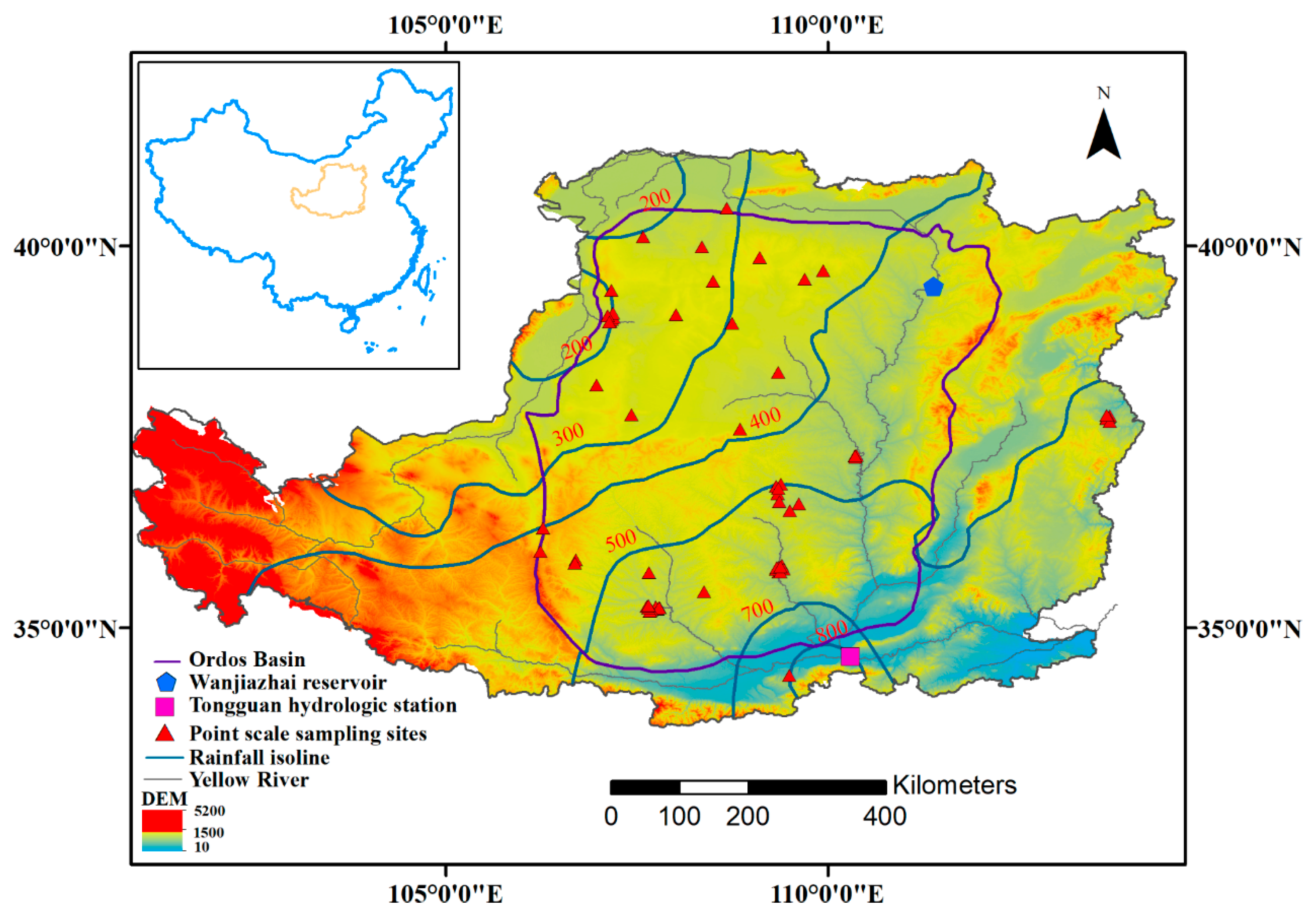
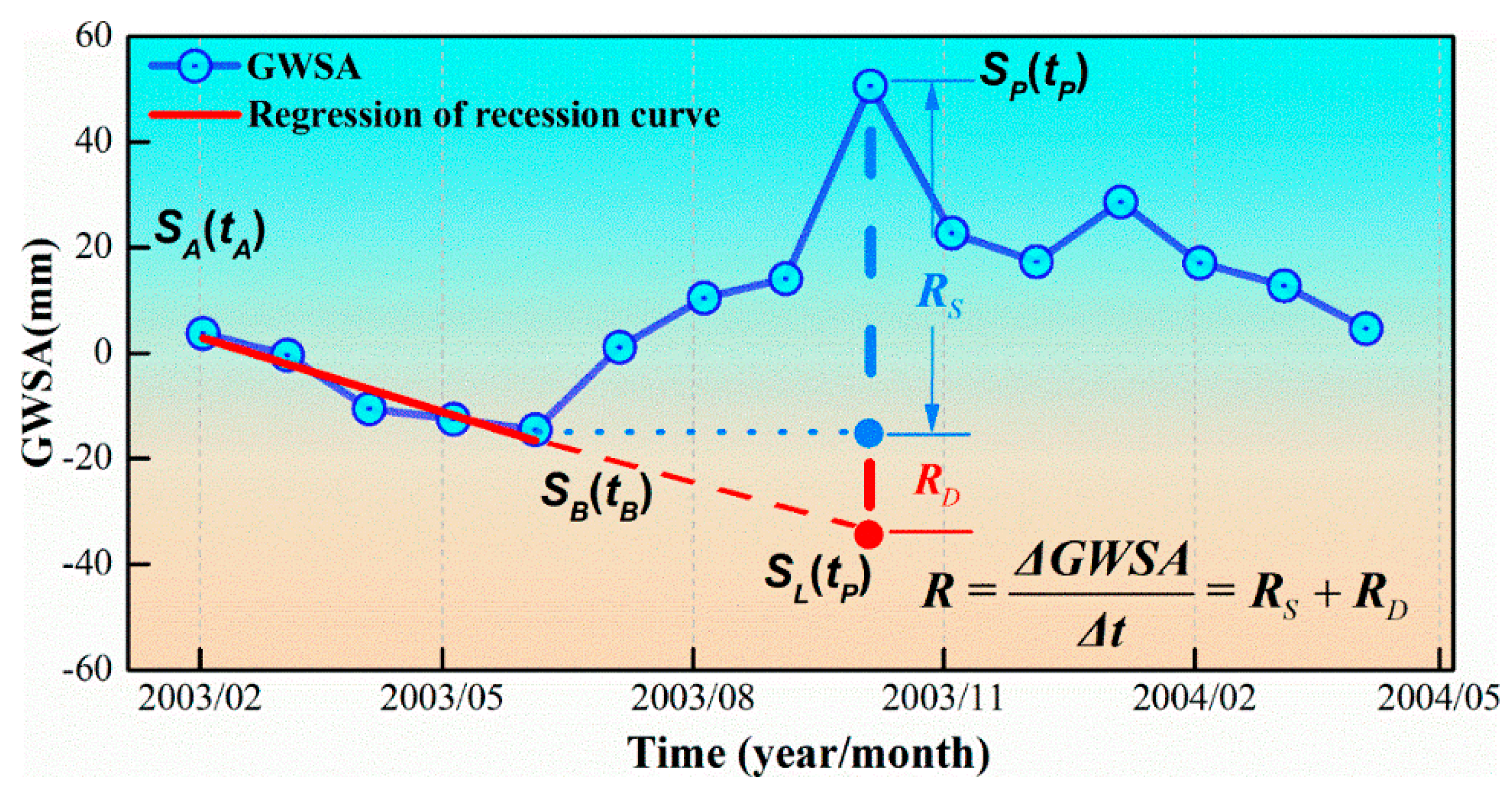
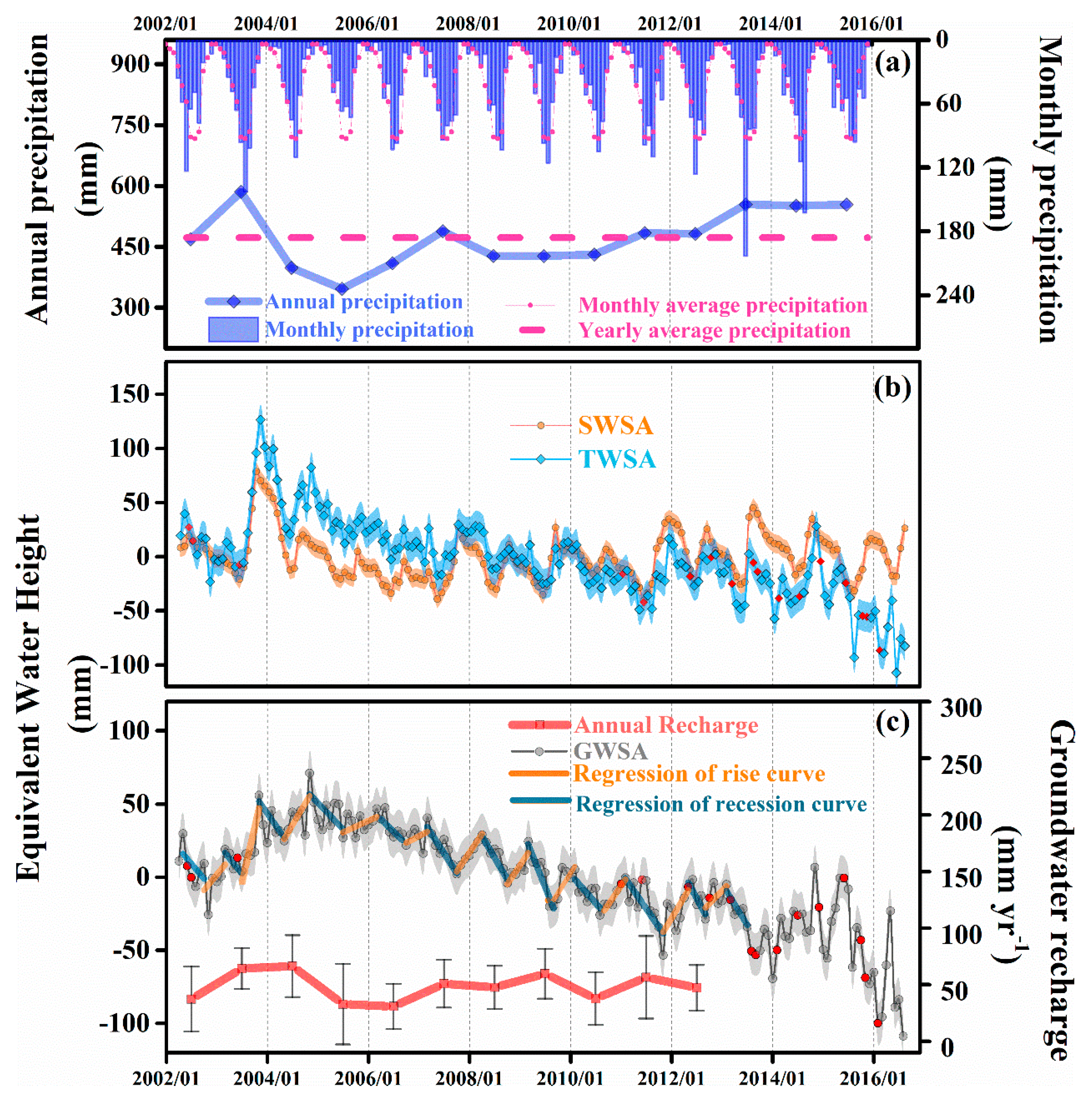
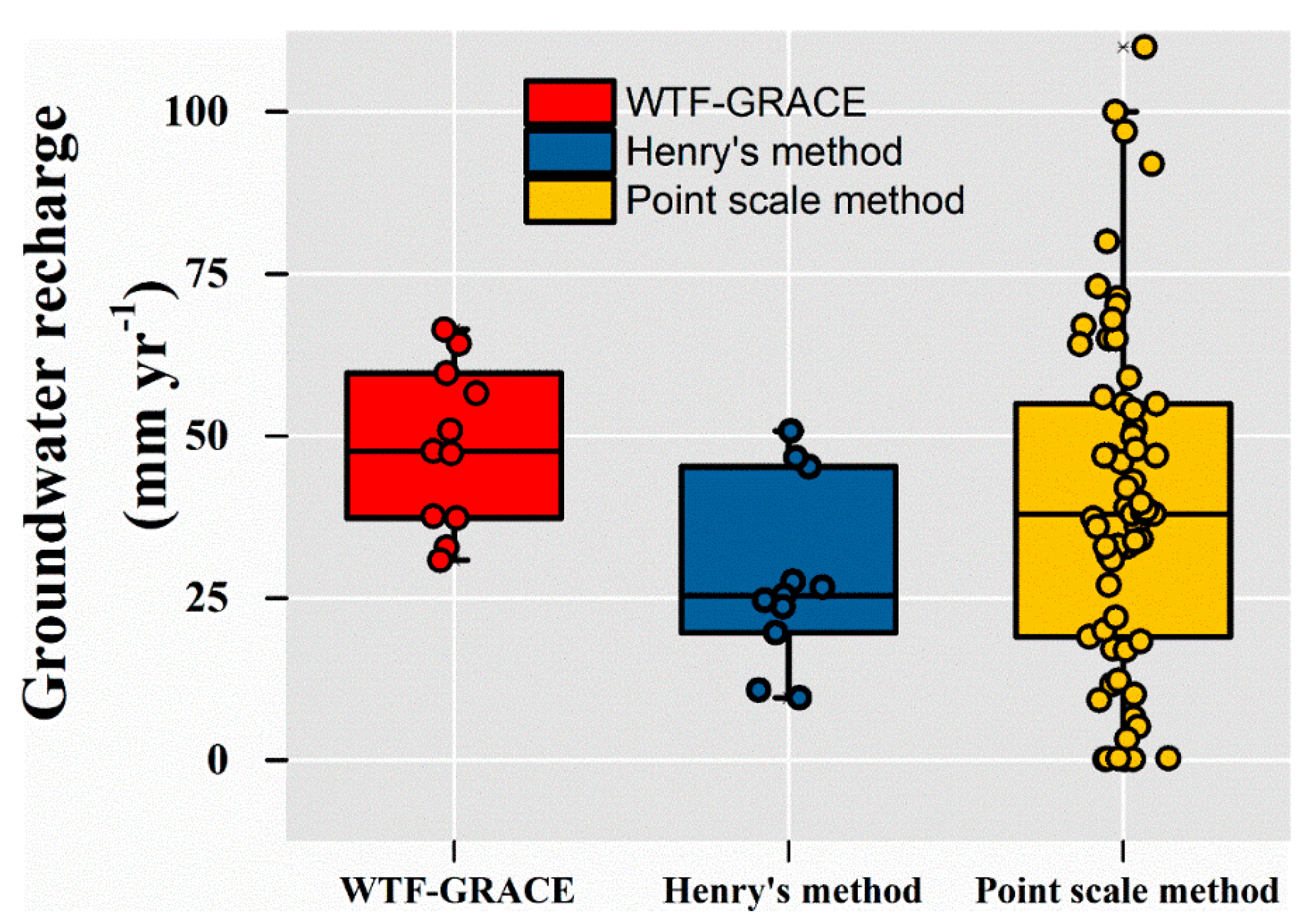
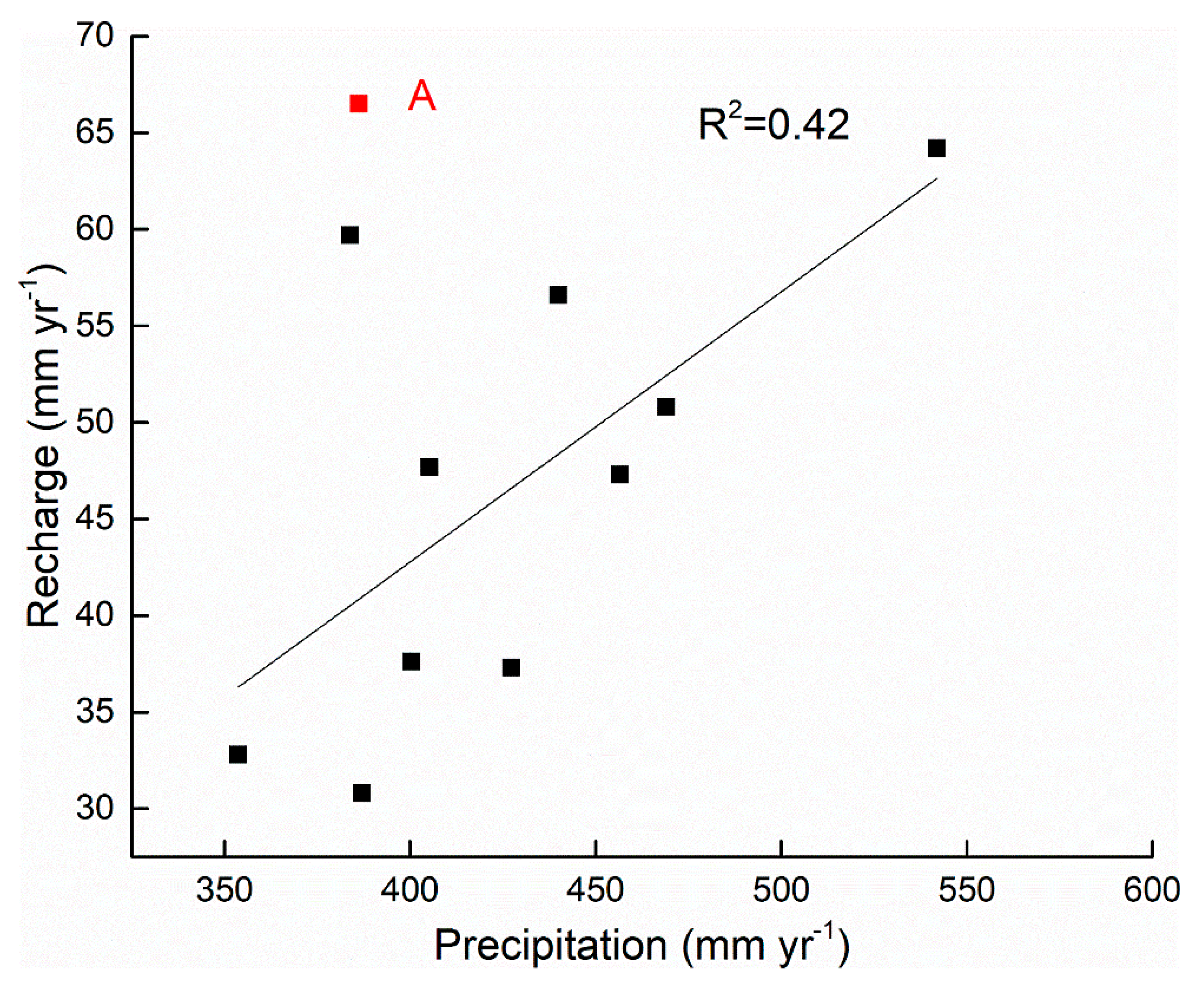
Table 1.
The variables used in estimating groundwater recharge from groundwater storage anomaly.
| Year | GRi (mm year−1) | N | R2 | ||||||
|---|---|---|---|---|---|---|---|---|---|
| 2002 | 19.1 | 14.9 | −18.2 | 23.7 | 37.3 | 28.7 | 5 | 0.52 | |
| 2003 | 56.2 | 14.9 | −8.1 | 8.0 | 64.3 | 18.1 | 4 | 0.66 | |
| 2004 | 71.3 | 14.9 | 4.9 | 22.2 | 66.4 | 27.5 | 6 | 0.50 | |
| 2005 | 46.9 | 14.9 | 14.1 | 31.7 | 32.8 | 35.6 | 8 | 0.36 | |
| 2006 | 40.7 | 14.9 | 9.8 | 11.9 | 30.9 | 20.1 | 6 | 0.46 | |
| 2007 | 29.1 | 14.9 | −21.8 | 13.5 | 50.9 | 21.1 | 6 | 0.81 | |
| 2008 | 24.5 | 14.9 | −23.1 | 10.0 | 47.6 | 19.0 | 5 | 0.89 | |
| 2009 | 5.4 | 14.9 | −54.3 | 15.0 | 59.7 | 22.1 | 5 | 0.88 | |
| 2010 | −0.4 | 14.9 | −38.0 | 16.7 | 37.6 | 23.3 | 6 | 0.53 | |
| 2011 | −6.5 | 14.9 | −63.2 | 32.8 | 56.7 | 36.6 | 6 | 0.63 | |
| 2012 | −4.9 | 14.9 | −52.2 | 12.0 | 47.3 | 20.2 | 5 | 0.68 | |
| Mean | 48.3 | 5.6 | 0.63 |
Note: represents the standard deviation of a certain variable, is the peak of the rise, is the GWSA extrapolated from antecedent recession curve at the time of the peak, GRi is the annual groundwater recharge. N is the number of sampling points used to fit the antecedent recession curve.
Table 2.
Different error components in estimating GR.
| Uncertainty | Equation | |
|---|---|---|
| 8.3 mm month−1 | (5) to (8) | |
| 14.9 mm month−1 | ||
| 7.7 mm year−1 | ||
| 0 mm year−1 | (9) | |
| 8.5 mm year−1 | ||
| 2.1 mm year−1 | ||
| 16.0 mm year−1 | (10) | |
| CV | 33.1% | (11) |
Note: Please see Table 1 for other calculation details.
© 2019 by the authors. Licensee MDPI, Basel, Switzerland. This article is an open access article distributed under the terms and conditions of the Creative Commons Attribution (CC BY) license (http://creativecommons.org/licenses/by/4.0/).
Share and Cite
MDPI and ACS Style
Wu, Q.; Si, B.; He, H.; Wu, P. Determining Regional-Scale Groundwater Recharge with GRACE and GLDAS. Remote Sens. 2019, 11, 154. https://0-doi-org.brum.beds.ac.uk/10.3390/rs11020154
AMA Style
Wu Q, Si B, He H, Wu P. Determining Regional-Scale Groundwater Recharge with GRACE and GLDAS. Remote Sensing. 2019; 11(2):154. https://0-doi-org.brum.beds.ac.uk/10.3390/rs11020154
Chicago/Turabian StyleWu, Qifan, Bingcheng Si, Hailong He, and Pute Wu. 2019. "Determining Regional-Scale Groundwater Recharge with GRACE and GLDAS" Remote Sensing 11, no. 2: 154. https://0-doi-org.brum.beds.ac.uk/10.3390/rs11020154
Note that from the first issue of 2016, this journal uses article numbers instead of page numbers. See further details here.