Article

Study of the Seasonal Effect of Building Shadows on Urban Land Surface Temperatures Based on Remote Sensing Data

1
State Key Laboratory of Earth Surface Processes and Resource Ecology, Faculty of Geographical Science, Beijing Normal University, Beijing 100875, China
2
Beijing Key Laboratory of Environmental Remote Sensing and Digital Cities, Beijing Normal University, Beijing 100875, China
3
Beijing Advanced Innovation Center for Future Urban Design, Beijing University of Civil Engineering and Architecture, Beijing 100044, China
*
Author to whom correspondence should be addressed.
Submission received: 17 January 2019 / Revised: 22 February 2019 / Accepted: 25 February 2019 / Published: 1 March 2019

Abstract

:
Building shadows (BSs) frequently occur in urban areas, and their area and distribution display strong seasonal variations that significantly influence the urban land surface temperature (LST). However, it remains unclear how BSs affect the LST at the city scale because it is difficult to extract the shaded area at the subpixel scale and to connect such areas with the LST at the pixel scale. In this study, we combined the sun angle, building height, building footprint and building occlusion to extract the seasonal spatial distribution of BSs in the central area of Beijing. The effect of BSs on the LST was analyzed using LST retrieved from Landsat-8 thermal infrared sensor data. First, the relationship between the LST patch fragmentation and proportion of BSs in the sample areas was modeled without vegetation. Then, we quantitatively studied the mitigated intensity of the LST in pure impervious surfaces (IS) and vegetation pixels covered by BSs; next, we analyzed the LST sensitivity of these pixels to BSs. The results showed that the existence of BSs influences the fragmentation of the low LST patches strongly from summer to winter. On the other hand, pure IS pixels totally covered by BSs experienced a greater cooling effect, with 3.16 K on 10 July, and the lowest cooling occurred between 14 and 25 December, with a mean of 1.24 K. Without considering the relationship in winter, the LST is nonlinearly correlated to the building shadows ratio (BSR) in pixels, and an approximate 10% increase in the BSR resulted in decreases in the LST of approximately 0.33 K (mean of 16 April and 10 May), 0.37 K (10 July) and 0.24 K (28 September) for pure IS pixels, and 0.18 K, 0.20 K and 0.15 K, respectively, for pure vegetation pixels. Further analysis indicates that the LST of pure IS pixels is more sensitive to BSs than that of vegetation because the self-regulation mechanism of vegetation reduces the cooling effect of BSs. These findings can help urban planners understand the cooling characteristics of BSs and design suitable urban forms to resist urban heat islands (UHIs).

1. Introduction

Urbanization changes the thermal energy exchange over the ground [1], causing many environmental issues in modern cities, including urban heat islands (UHIs). A UHI occurs when the urban air or surface temperature is higher than the suburban temperature due to a large number of artificial buildings and less vegetation [2]. A series of urban environmental problems have arisen, exacerbating reductions in water and air quality, accelerating energy consumption and increasing the violence and mortality of humans, thus making it imperative to reduce UHI effects [3].
Three factors influence UHIs: (1) natural elements; (2) the urban composition and configuration; and (3) the socioeconomic index [4,5]. Most previous studies focused on the relationship between the three factors and urban land surface temperature (LST) using qualitative or quantitative methods based on remote sensing data [6,7,8,9,10,11]. Among them, the urban form is an effective method of mitigating UHI [7], although few studies have focused on this method, especially the three-dimensional features of buildings [12]. The building density, sky view factor (SVF) and other factors have been modeled with urban LST [13,14]. However, except the factors mentioned above, scholars have provided only a limited exploration of how building shadows (BSs) affect LST at the city scale, which is a crucial element affecting the local-scale UHI variations and urban thermal environment [15].
Previous research has shown that solar radiance must be alleviated by BSs in summer [16]. As a special urban surface component that is closely related to the building structure and distribution, BSs have effectively improved urban thermal environment by preventing solar radiation from penetrating into the street canyon [17]. To date, most research focuses on the cooling effect of BSs through analyses of urban thermal comfort [18,19,20,21,22]. Watanabe evaluated outdoor thermal comfort during summer and indicated that building shade provided cooler thermal environments with universal effective temperature (ETU) reductions of 18.4 °C at 800 W/m2 of total solar radiation in sunlight [23]. Hwang conducted field experiments and revealed that, from spring to autumn, the best thermal comfort appeared under street shadows; however, in winter, areas without shadow feel more comfortable, which might due to the sufficient solar radiance [24]. In addition, other studies utilized the W/H (street width/building height) ratio and sky view factor (SVF) between nearby buildings to assess the shading levels [25,26,27,28]. Discussing the cooling effect of BSs from the perspective of thermal comfort is the main direction of current research. Several studies have discussed the thermal performance of buildings under adjacent shading [29,30]. For example, an analysis by Chan suggested that building thermal performance is significantly influenced by shadows from surrounding trees and buildings [31]. Experiments in Hong Kong by Lam indicated that the building cooling loads decreased by approximately 2% due to the shadows of nearby buildings [32].
However, numerous studies on the cooling effect of BSs are based on thermal environments that are determined by fixed point measurements, modeled simulations and manual surveys, which only represent phenomena at microscales such as independent buildings, streets and communities and do not focus on the direct cooling effect of BSs on urban LST in pixels at the macroscale or expand on the temporal scale.
Compared with in situ measurements, remote sensing could provide more complete, continuous and uniform sampling, especially for the spatiotemporal dynamics of surface features, which are widely used in UHI analysis [33]. Moderate Resolution Imaging Spectro radiometer (MODIS) and Landsat Operational Land Imager (OLI) have been used to demonstrate the cooling effect of the above factors from the perspective of remote sensing. Unfortunately, for medium- and low-resolution images, BSs are always excluded as noise [34,35], which results in a limited understanding of BSs and incomplete determinations of factors mitigating UHI. With the occlusion of solar radiance by buildings, BSs are regarded as a non-negligible component at the city scale. In addition to natural surfaces, the existence of BSs also makes the land surface become an urban cool islands (UCI) on the macro scale, especially in areas with high building density [33]. Such areas have more significant seasonal variations, which is partially due to (1) the variation of the solar azimuth and solar elevation angles making shaded areas change dramatically in urban regions compared to vegetation; and (2) the seasonal regulation of solar radiance changing the temperature difference between shaded and nonshaded land surfaces. The above two points confirm the distribution of BSs and their effect on urban LST have significant temporal uncertainty, and therefore, must be addressed under these conditions, which has been rarely noted in previous studies. Therefore, as an urban form factor, it is crucial to analyze the cooling effect and seasonal characteristics of BSs to determine the impacts of urban form on UHI.
Considering the above issues, our study focuses on the seasonal cooling effect of BSs on urban LST at the pixel scale instead of at the micro scale. The seasonal variation of thermal landscape fragmentation under the influence of BSs is discussed and reveals the distributed variation of LST patches caused by the disturbance of BS cooling. Then, the cooling intensity of pure impervious surface (IS) pixels totally covered by BSs is simulated via an interpolation of different seasons, and the BSR in pixels was calculated to enable an analysis of changes in the LST of pure IS and vegetation pixels with increases of the BSR, as well as further comparisons of their difference. The abovementioned studies were conducted within the fifth loop of Beijing. The Landsat-8 datasets on 25 December 2014, 16 April 2015, 14 December 2016, 7 May 2017, 10 July 2017 and 28 September 2017 were utilized to calculate LST, while the pixels of BSs could be extracted with SPOT-6 digital surface model (DSM) data on 1 January 2016. Eventually, we produced 14 figures to express the results of this study. Based on these works, the seasonal contribution of BSs to the mitigation of the UHI at the macro scale could be well represented.

2. Materials and Methods
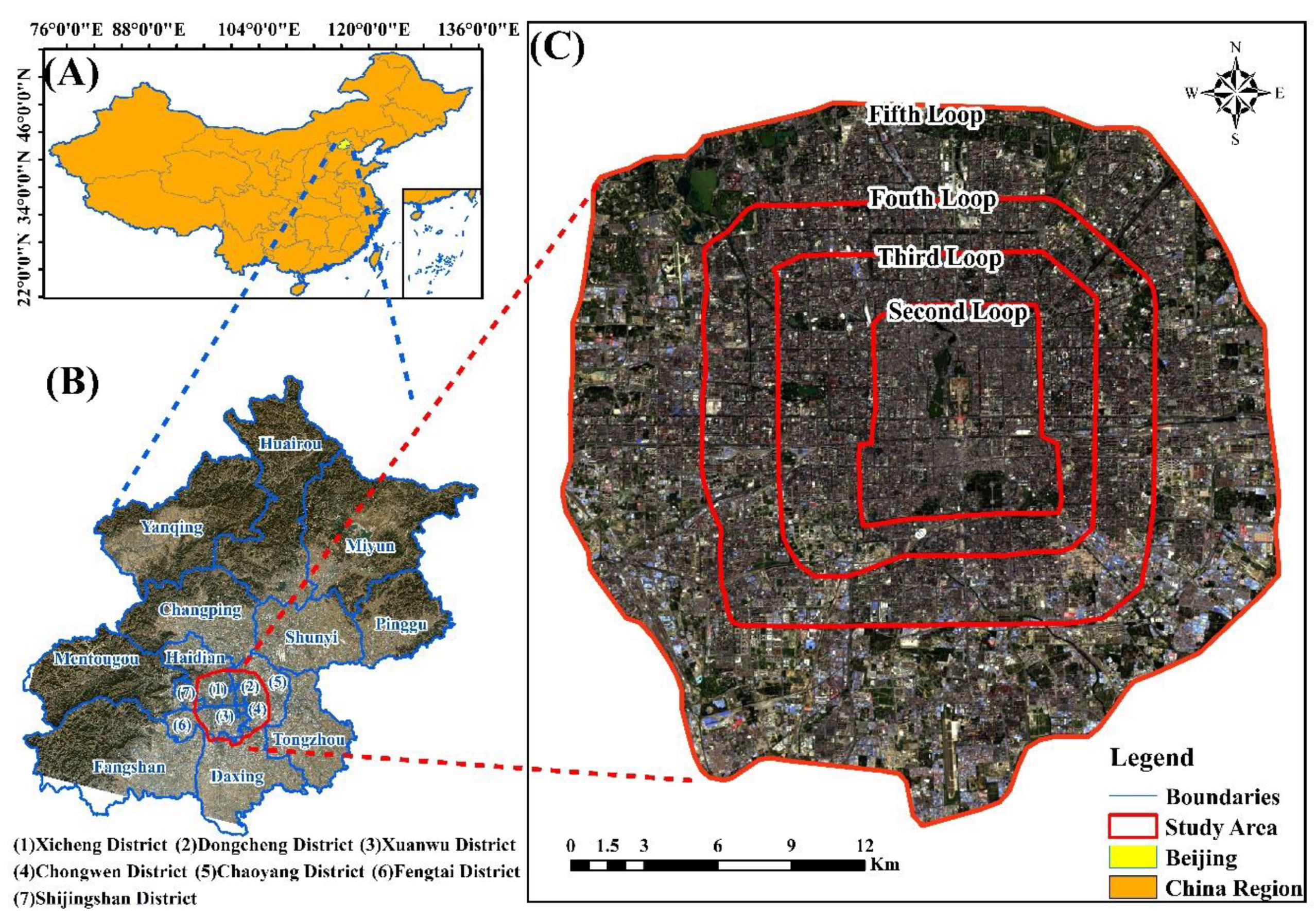
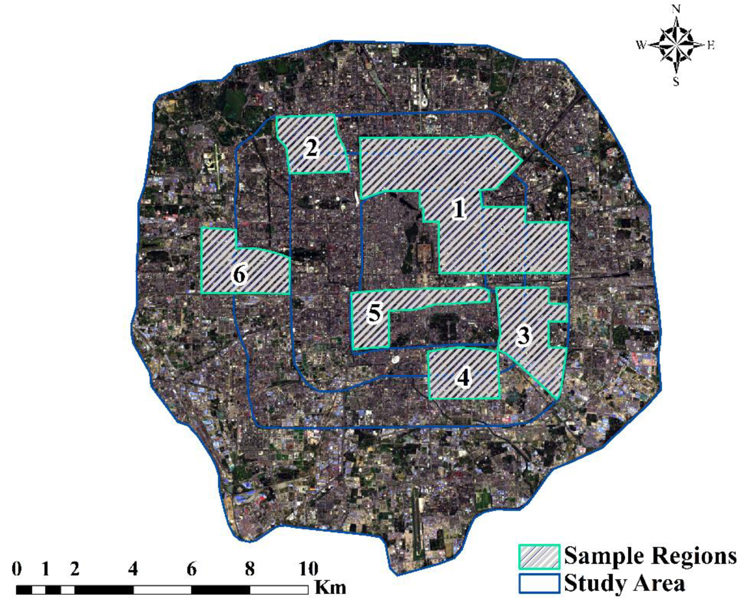
2.1. Study Area

Beijing is the capital of China, and one of the world’s largest cities. It is located at 115.7–117.4°E and 39.4–41.6°N. The average altitude is 43.5 m, and it has a temperate monsoon climate. The annual precipitation is 640 mm and the annual average temperature is 12 degrees Celsius. In the past two decades, Beijing has experienced significant changes characterized by accelerated urbanization. Its development model is a typical concentric expansion, thus forming an obvious circular pattern from the inner center to the suburbs. The roads are mostly supported by this pattern, and they are distributed in parallel with the latitude and longitude lines in the second, third, fourth, fifth and sixth Ring Roads. This study is focused on the area within the Fifth Ring Road, which encompasses the location of the main city of Beijing, covering eight districts. The main area covers 666.02 km2 and consists of 9 counties and 12 townships (Figure 1).

2.2. Data

2.2.1. DSM Data

SPOT-6 Digital Surface Model (DSM) data were used to extract buildings and their shadow pixels from stereoscopic pairs acquired on 1 January 2016, via the Universal Transverse Mercator projection system (datum WGS84, UTM Zone N50). To obtain the building dataset of the study area, it was corrected with Digital Elevation Model (DEM) data. An ALOS PALSAR 12.5 m DEM was obtained from the ALASKA SATELLITE FACILITY (https://vertex.daac.asf.alaska.edu/). The approach was as follows: (1) the DEM (12.5 m) was converted into contours with a spacing of 1 m and the Delaunay Triangulation Net was constructed; (2) using Delaunay Triangulation, we obtained a 6 m DEM; and (3) the actual height of the features for certain pixels was calculated as the difference between the corresponding DSM and DEM pixels. Finally, we selected the landmark height in the study area to validate the accuracy of the DSM, and the R2 reached 0.9898, with a Root Mean Square Error (RMSE) of 3.84 m.

2.2.2. Landsat-8 Thermal Infrared Sensor Data
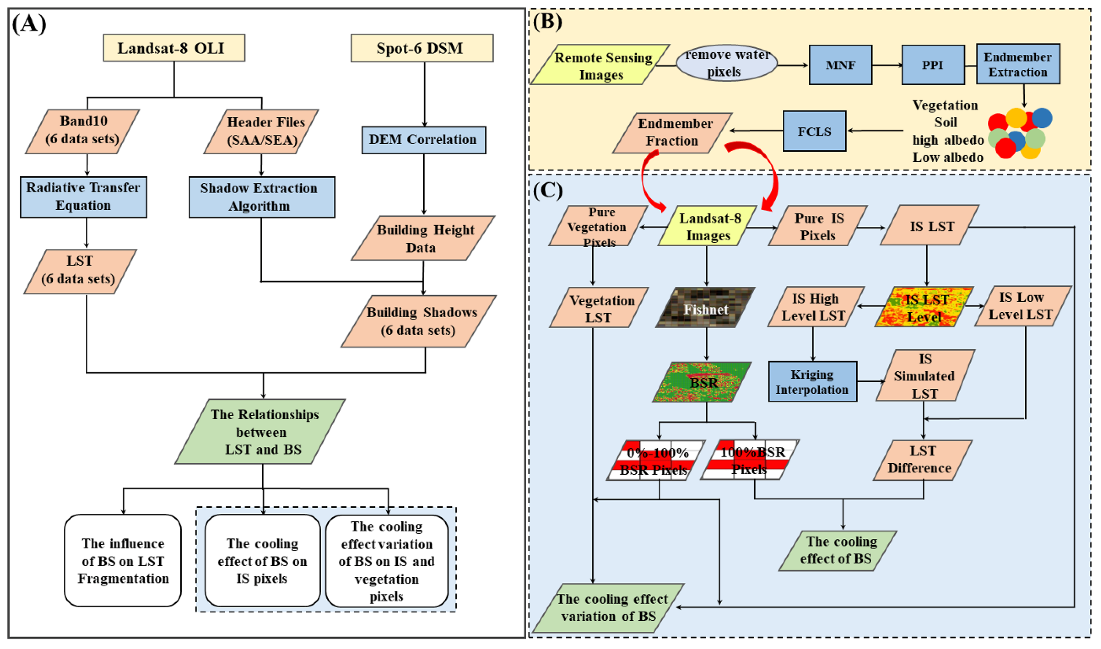
Landsat-8 thermal infrared sensor (TIRS) data were used to calculate the LST in our study with a resolution of 100 m. Data sets with no more than 5% cloud cover could be downloaded from the United States Geological Survey (USGS) (https://earthexplorer.usgs.gov/) to meet the needs of seasonal research; the details are displayed in Table 1. These data have a similar overpass time every day (approximately at 10:53 a.m. CST (China Standard Time)) so that the LSTs could be compared with each other. The solar azimuth angle and elevation angle (SAA and SEA, respectively) were obtained to extract the BSs pixels from DSM data and details can be found in Section 2.3.1. All Landsat-8 data were in the same projection system as the DSM data.

2.3. Methods

The study of the seasonal effects of BSs on LST was divided into the following steps (Figure 2). First, the LST of our study area was retrieved from Landsat-8. Then, DSM data extracted from SPOT-6 were used to obtain BS pixels, with the SAA and SEA from the header files of Landsat-8. Finally, we analyzed the relationships between BSs and LST from different aspects. The details are shown below in the description of the methodology. Note that the study focuses on pure IS pixels in Section 3.2 and Section 3.3.1, and on pure IS and vegetation pixels in Section 3.3.2 and Section 3.3.3.

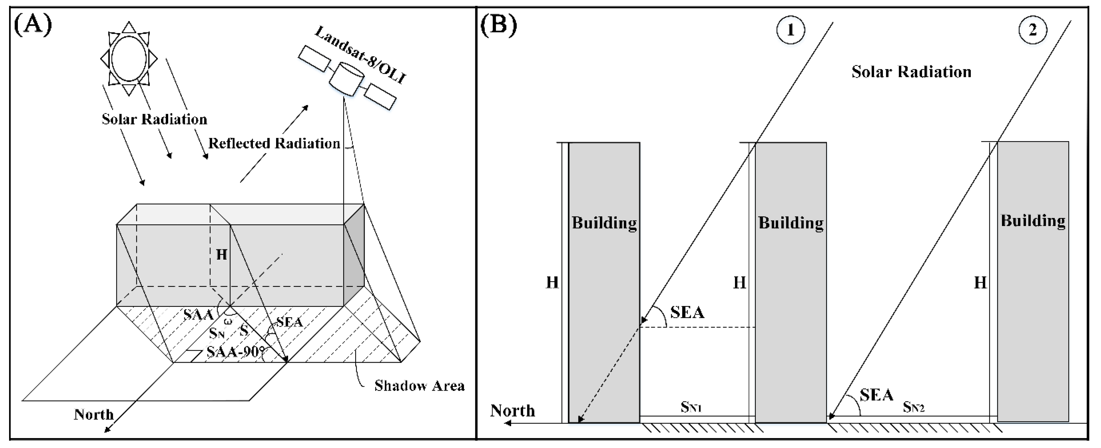
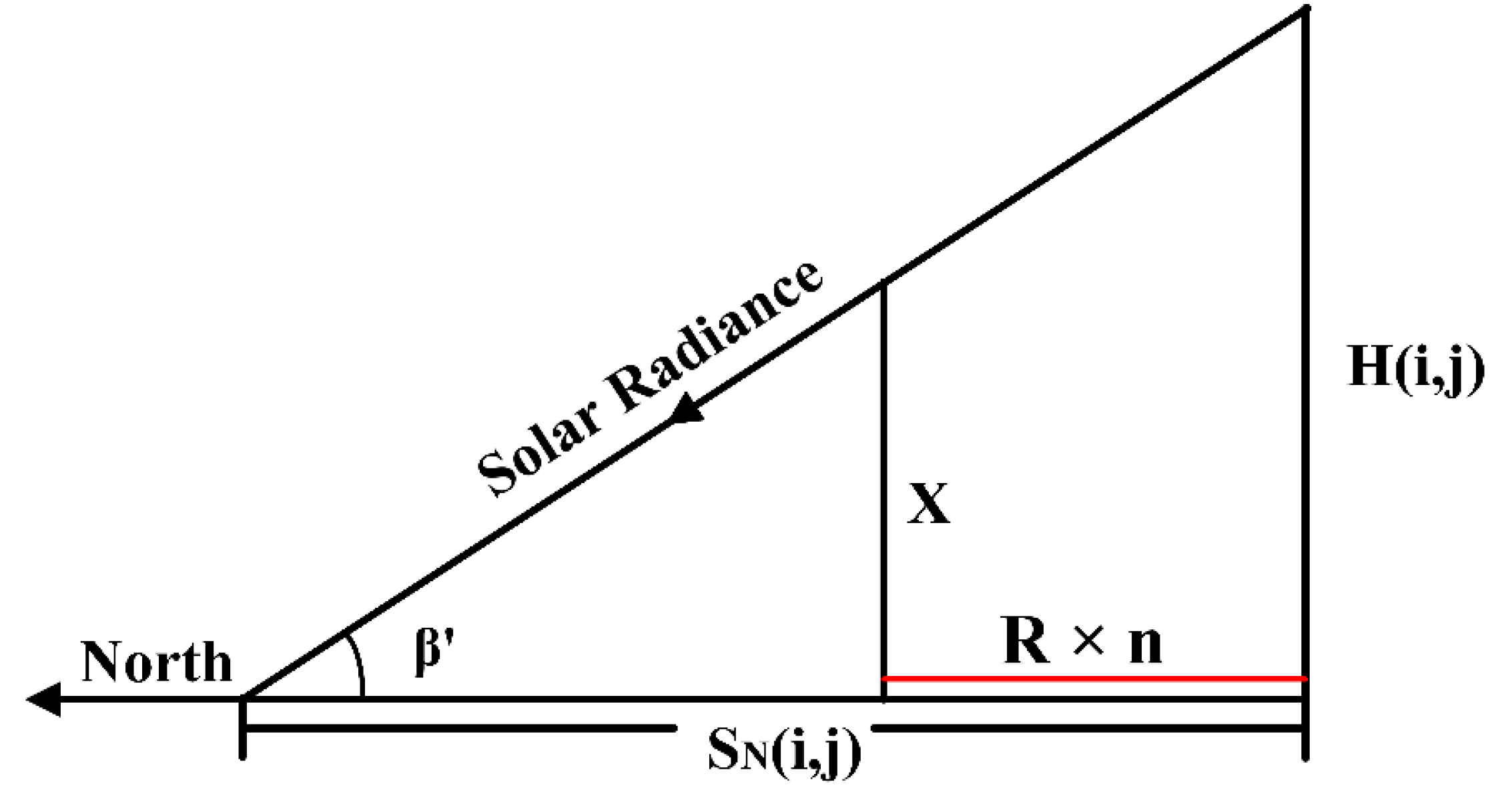
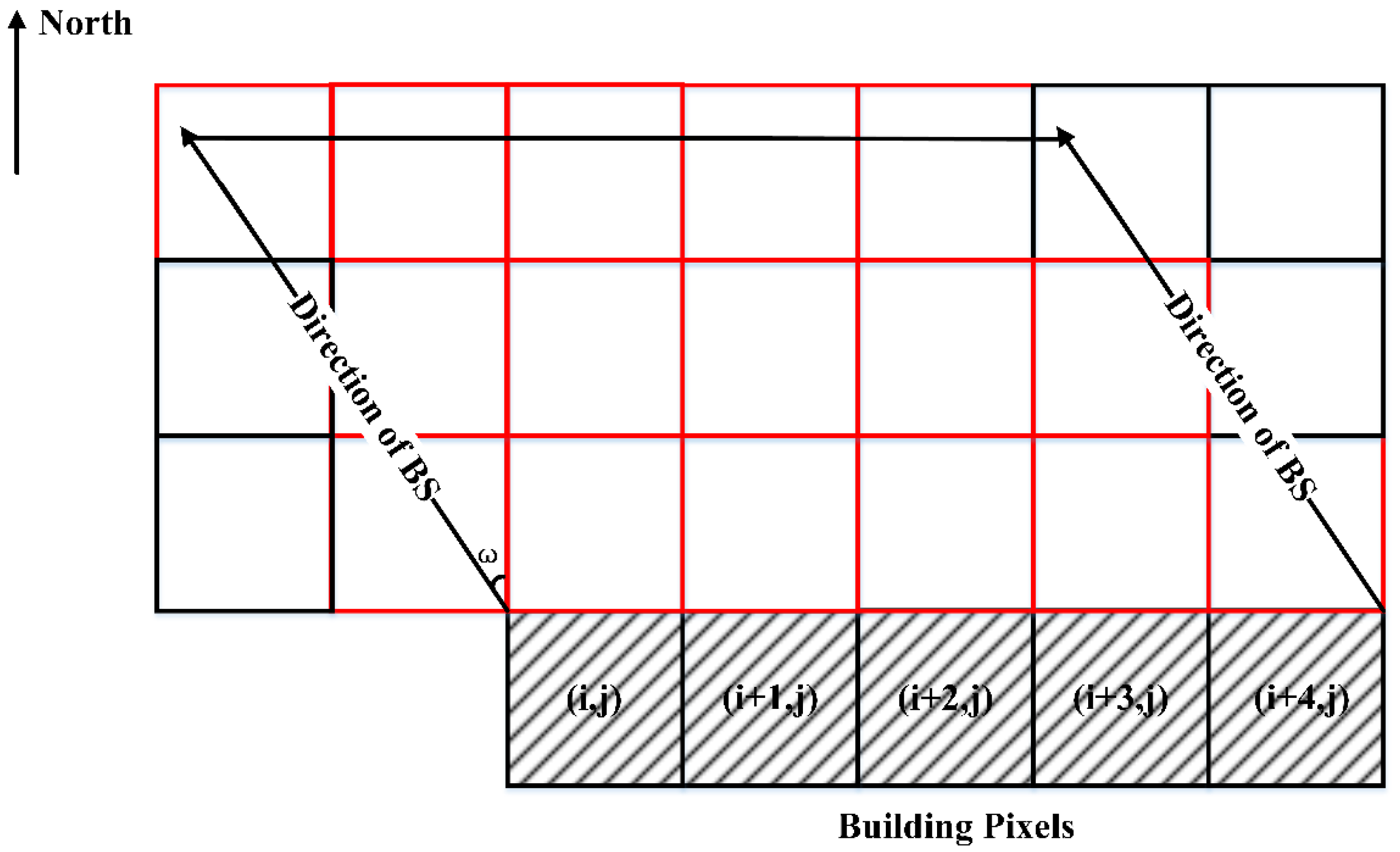
2.3.1. Extraction of Building Shadows

BS pixels from DSM data (6 m) were obtained according to the geometric relationships among the sun, buildings and remote sensors (Figure 3). As the high-resolution images limited the acquisition of data sources, which were unable to meet the needs of our multitemporal analysis, it was not feasible to extract BSs from such images at high resolution with the spectral characteristics used in many previous studies [36,37,38]. BSs are difficult to capture as a special type of surface in remote sensing images with medium and low resolution; thus, the true distribution of BSs is not reflected due to the region smoothing of pixels [39,40]. Therefore, we did not use images of Landsat-8 to extract BSs. For the classification of land cover, many scholars currently use spectral decomposition methods for mixed pixels, such as MESMA (Multiple Endmember Spectral Mixture Analysis) [41,42,43]; however, because of the insufficient amount of BS information, these pixels are often classified as other low-albedo classes [34], such as asphalt road and water. Moreover, we tried to perform mixed pixel decomposition under the premise of excluding water, although the accuracy was difficult to control due to the complexity of the IS spectrum in the study area. For example, roads with lower albedo might be covered by BSs, but their similar spectral characteristics led to a large classification error; thus, we could not separate BSs from other low-albedo IS pixels, and this method was excluded.
The theoretical expression of the simplified model is as follows [44]:
S = H/tan SEA
SN = S × sin (SAA − 90°)/R
where H is the building height; S is the length of shadow on the ground; SN is the number of pixels occupied by the projection of S in the north direction; and R represents the spatial resolution of DSM data. The correlation of S and SN which expressed by Equation (2) could be founded in Figure 3A.
Our calculations were performed for pixels of DSM data. Combined with Equations (1) and (2), the formula for SN was as follows:
SN (i, j) = (H (i, j) × sin (SAA−90°) / (R ×tan SEA))
SN (i, j) is the SN for the pixel in row i and column j; and H (i, j) is the DSM value of pixel (i, j).
Then, we judged the actual SN (i, j) in the image matrix because of the shading effect of surrounding buildings (Figure 4). In addition, (i, n) is the pixel that is n pixels away from (i, j) in the north direction, and the formula for X is as follows:
X = ((SN (i,j) − R × n))/(SN (i,j)) × H(i,j)
where X is the criterion for whether (i, n) is obscured by the BSs of (i, j); n represents the number of pixels between (i, j) and (i, n); R × n is the distance between building pixels; and SN (i, j) and SN (i, j) are the same as above, with the former from Formula (3).
According to the geometric relationship; for the pixel (i, n), if H (i, n) is greater than or equal to X, then the actual SN (i, j) is equal to R × n; and if H (i, n) smaller than X, then the actual SN (i, j) is equal to SN (i, j). Through the above steps we can extract the true shadow length in the north direction.
After ensuring the number of BS pixels in the north, we determined the position of pixels covered by BSs for one building according to the SAA in different seasons (Table 1). Specifically, we could obtain the angle between the north direction and the solar incident direction for buildings, which represented by ω in Figure 3A. Then, we could obtain the pixels that the BSs might cover by utilizing the relationship between the tan (ω) angle and the side length of DSM pixels (Figure 5). Notes that if the occupied area in one pixel was no more than 1/3 of pixel, such pixels would be removed. We regarded each building pixel as a single building, and extracted BS pixels in line with SN and tan (ω).
It is worth mentioning that the DSM might include the elevation of roads, mountains and vegetation, which might increase the errors of the results. Hence, we artificially drawn building polygons with high-resolution Google Earth images (1 January 2016) as a building discrimination basis to accurately extract BS pixels. Note that the Landsat-8 data acquisition time was not consistent with the DSM time; thus, we assumed that the height of the buildings within the study area did not change within three years and the BS pixels at different times could be extracted according to the SAA and SEA in Table 1.

2.3.2. LST Retrieval from Landsat-8 Thermal Infrared Sensor Data

The radiative transfer equation (RTE) was exploited to calculate LST. The accuracy of this method is lower than 1 K in natural surfaces and reached approximately 2.8 K in heterogeneous surfaces such as urban areas [45,46,47]. It could be utilized in our study to retrieve the LST of six datasets (Landsat-8) with the thermal infrared band 10. Details can be found in García- Santos [47], and the main formula is as follows:
B(LST) = (Lλ − L − τ × (1 − ε) × L)/(τ × ε)
LST = K2/ln(K1/(B(LST)) + 1)
where B(LST) is the blackbody radiance under temperature LST; Lλ is the thermal infrared radiance (W⋅m−2⋅sr−1⋅m−1) acquired by radiance calibration [48]; L, L, and τ are the upwelling, downwelling atmospheric radiance and transmittance of the atmosphere in the thermal infrared band, respectively, retrieved from the NASA website (http://atmcorr.gsfc.nasa.gov/); and ε is the land surface emissivity (LSE). For Landsat-8/OLI sensors, K1 = 774.89 W/(m2·sr·m), and K2 = 1321.08 K.
The threshold method was used to estimate ε [46]. Land cover was classified by the normalized difference vegetation index (NDVI), and the ε of every type could be estimated. Specifically, urban surfaces can be considered a mixture of architecture and vegetation, and natural surfaces can be considered a mixture of vegetation and bare land. The main equations of ε were as follows:
  ε n = P v R v ε v + ( 1 P v ) R s ε s + d ε
  ε a = P v R v ε v + ( 1 P v ) R m ε m + d ε
where R v ,   R s and R m   are the temperature ratio of vegetation, bare land and architecture, respectively. ε n ,     ε a , ε v , ε s ,   and   ε m are ε of natural surfaces, urban surfaces, vegetation, bare land and architecture, respectively; and P v   is vegetation coverage. The R could be calculated as follows:
  R v = 0.9332 + 0.0585 P v
  R s = 0.9902 + 0.1068 P v
  R m = 0.9886 + 0.1287 P v
After estimating NDVI max and NDVI min in each Landsat image we could obtain P v . The equation was as follows:
  P v = [ NDVI NDVI min NDVI max NDVI min ] 2
In the above equations, ε v = 0.986 , ε s = 0.972 ,   ε m = 0.970 ,   and   d ε is a parameter of the land surface feature, which we regarded as zero. According to the formula above, ε could be retrieved.

2.3.3. Definition of Thermal Landscape Fragmentation

Landscape fragmentation refers to a patch divided into relatively small areas that are not connected with each other [49]. Previous studies have selected landscape metrics to describe thermal landscape fragmentation [50,51]. To analyze the influence of BSs on the fragmentation of the thermal landscapes of the study area, we divided the LST into five categories using the mean-standard deviation method [52]. The temperature range for each category is shown in Table 2. Frastats4.0 was utilized to calculate percentage of landscape (PLAND), number of patches (NP) and patch density (PD) of every LST class, which could represent the distribution characteristics of LST [53].
The PD included the landscape and class patch density [54]. The former is the NP of all heterogeneous landscape classes per unit area (PD) and the latter is the NP of every landscape class per unit area (PDi). A higher PD means the patches are more isolated. In our study, we only discuss the PDi of five LST classes. Details about the metrics are shown in Table 3.
The cooling effect of natural surfaces (vegetation and water) might interfere with the analysis of BSs, and if we directly removed the pixels of natural surfaces, continuous IS would become broken, thereby reducing the accuracy of the calculation of PD calculations. Therefore, we selected six sample regions to compute the PDi and BSR. These regions are all in the main city and the influence of natural surfaces can be ignored. The details of the sample regions are as follows (Figure 6). These samples were distributed as evenly as possible in the main city. In the fifth loops, there are not enough areas of high-rise buildings and the natural surfaces occupied a considerable area, hence, we selected few samples in this region. The areas of the six samples are 52.12 km2, 10.21 km2, 15.60 km2, 10.52 km2, 11.50 km2 and 13.59 km2. We used these polygons to clip the LST-class images and BS datasets obtained in Section 2.3.1 and Section 2.3.2. The PD and BSR in six samples were calculated and the relationships were described using statistics.

2.3.4. Extraction of Pure Is and Vegetation Pixels

The spectral smoothing effects of pixels with 30m resolution in urban areas c may lead to serious underestimations in the true distribution of BSs in medium-resolution images [55]. Meanwhile, it is difficult to separate BS pixels from low-albedo pixels using pixel unmixing method (Section 2.3.1). To describe the cooling effect of BSs and exclude the influence of other features on LST, we first identified and extracted pure pixels (vegetation and IS), including those covered by BSs, employing the fully constrained least squares (FCLS) method [56,57]. The distribution of BSs in pixels (30 m) could be extracted by combining shadow layers separately obtained with SPOT-6 datasets (6 m). The details are as follows.
Since the study area is relatively small and the spectral similarity of water and shadows might cause errors in calculating modified normalized difference water index (MNDWI), we used artificial vectorization to remove water bodies to reduce noise. Then, we regarded land cover types as vegetation, soil and IS after masking the water bodies because we focus on the influence of BSs on IS and less on the analysis of vegetation; thus, all the IS categories were combined into two classes, with roads, cements, concrete surface and tile in the lower albedo class and glass and metal materials in the higher albedo class [58]. The forests and green spaces were integrated as vegetation for the analysis to ensure a sufficient number of pixels. First, according to the spectral characteristics of our study area, we used a four endmember model (vegetation, soil, low albedo, high albedo) to select pure pixels of different categories [59]. Note that IS and vegetation pixels with BSs belong to low-albedo and vegetation categories, respectively, according to previous research [60]. The endmember extraction of four categories of four categories was performed based on the combination of Minimum Noise Fraction Rotation (MNF) and Pixel Purity Index (PPI) methods [61].
Finally, The FCLS spectral unmixing method was used to calculate the endmember proportion in pixels, and details about this algorithm can be found in Li [56]. The total proportion of high and low albedo categories were considered as IS proportions [59]. To determine a sufficient amount of data, pixels with IS proportions greater than 80% were classified as pure IS pixels, and a similar criterion was applied to pure vegetation pixels. Notably, factories with blue or red roofs in the southern study area were wrongly divided into soil due to the spectral similarity; however, measures to reclassify them as IS pixels were not applied because these factories had lower building heights and thus did not form BSs. In addition, the higher LST of factories increased the spatial heterogeneity of temperature. Hence, we omitted these pixels to reduce LST uncertainty. The extracted results are shown in Table 4. In winter, we did not have enough vegetation pixels to analyze; therefore, the datasets on 14 and 25 December were excluded from this analysis.
The locations of random pure IS and vegetation samples were manually identified using high-resolution Google Earth images to validate the classification accuracy. We selected 3403 pure IS pixels and 1047 vegetation pixels, and the obtained mean matching accuracies were 83.36% and 87.44%, respectively.

2.3.5. Quantification of the Cooling Effect of BSs from LST Data

After obtaining pure pixels, we simulated the cooling effect of BSs and compared the differences between IS and vegetation pixels. The details are as follows.
(1) We covered the entire study area with 30 m grids corresponding to pixels of Landsat-8 data. (2) The BS layers obtained in Section 2.3.1 were applied to calculate the BSR in every pure IS pixel. (3) Meanwhile, temperature class images (Section 2.3.3) occupied by pure IS pixels were extracted, after removing sub-low and low LST pixels, which might correspond to BS pixels. (4) We assume that pixels with higher temperatures were contaminated by few BSs. As such, the LST of IS pixels that were removed in step (3) could be simulated through interpolation using the Kriging method. (5) The effect of BSs on the LST can be expressed as the difference between the simulated temperature of a pure IS pixel and its real temperature retrieved in Section 2.3.2. Finally, pixels that were totally covered by BSs with aBSR of 100% were extracted to obtain the temperature difference between BSs and non-BSs pixels.
Because the cooling effect of BSs on LST might be strongly affected by variations of the BSR in pixels, and IS and vegetation are most likely to show diverse responses to BSs due to their thermal characteristics, we utilized 30 m grids to estimate the BSR in pure IS or vegetation pixels directly because we had no method of interpolating the LST of vegetation pixels by Kriging in the same way as IS. Then, we counted the LST of these grids in different BSR intervals to represent the temperature variation. We used a statistical method for IS and vegetation to replace the interpolation method for two reasons. First, the pixels covered by BSs and vegetation all belong to low-level LST patches (Section 3.2), which might have relatively close temperature s; hence, utilizing the Kriging method for vegetation to calculate the LST difference increased the difficulty of ensuring the credibility of the results. Second, the existence of mixed pixels might increase the extraction errors of vegetation, thus leading to incorrect interpolation results that could not be controlled for. Hence, pixel statistics represents a better method and was used to represent the effect of changes in BSR on the LST in pure IS and vegetation pixels. Note that for IS pixels, the Kriging interpolation was replaced with the statistical method to better compare the cooling difference of BSs between IS and vegetation pixels.

3. Results

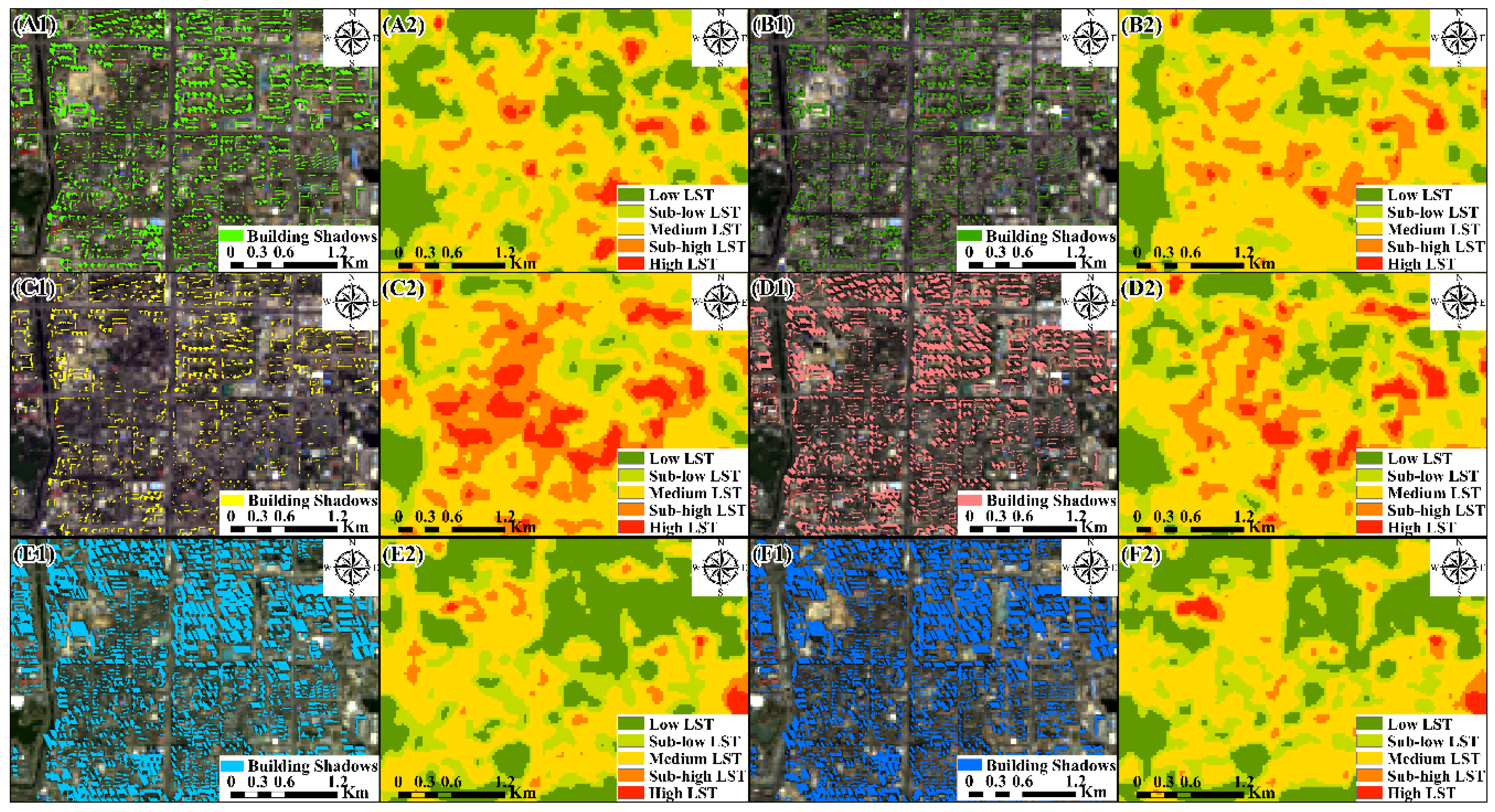
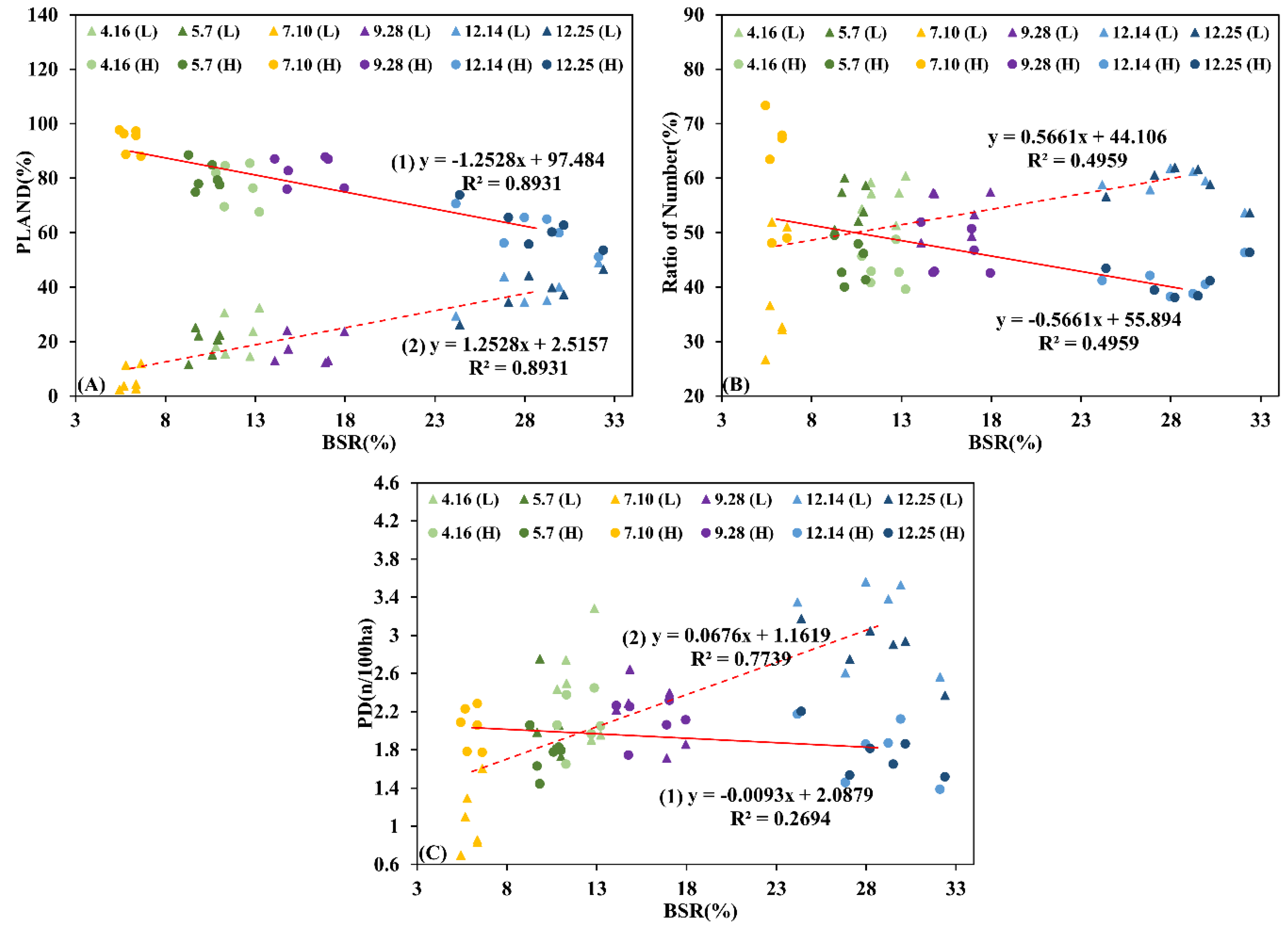
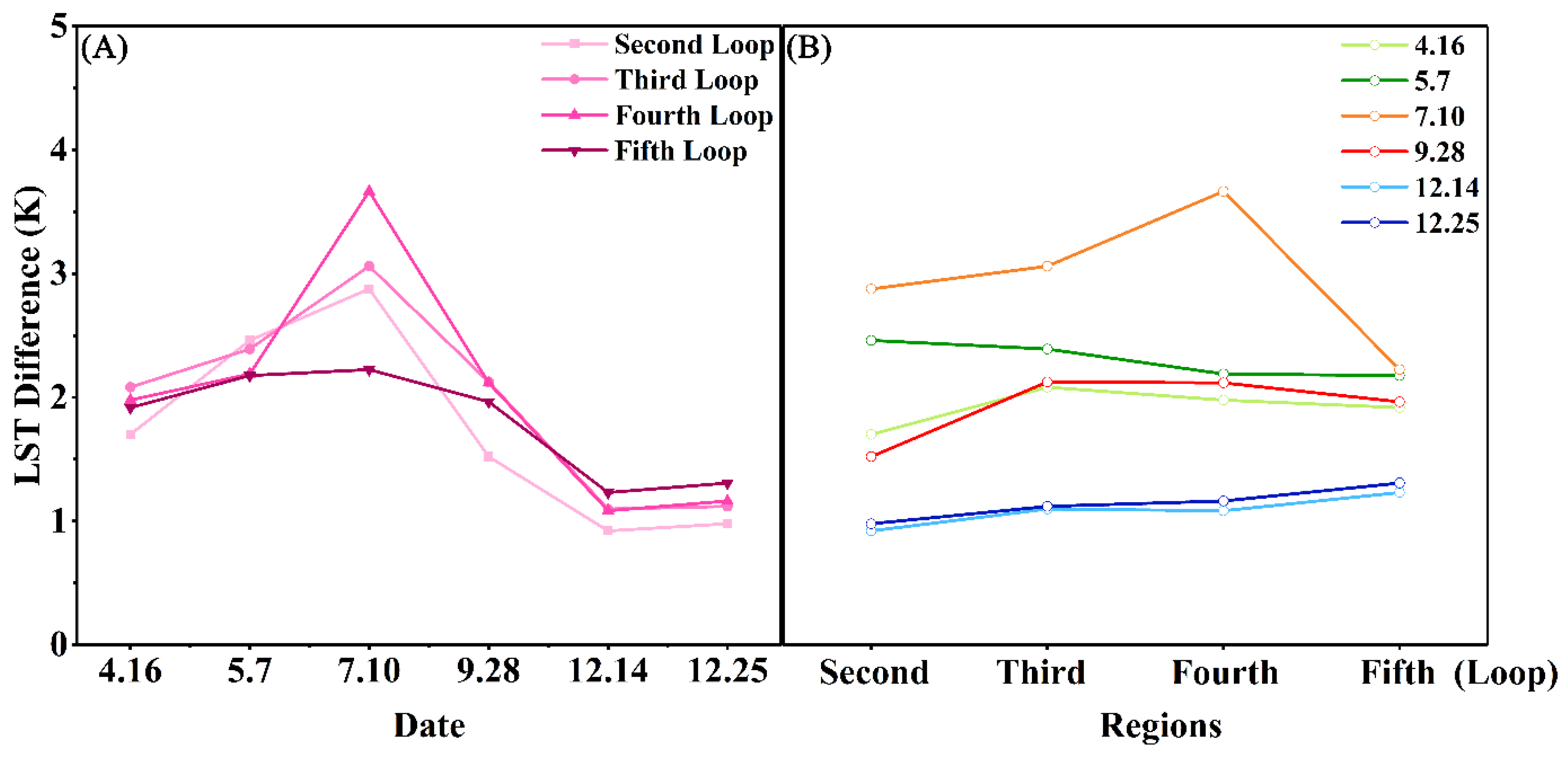
3.1. Seasonal Characteristics of BSs Areas and LST

The spatial distribution of BS pixels and LST in different seasons is shown in Figure 7. In our study, the available datasets were divided into four seasons: 16 April and 7 May for spring; 10 July for summer; 28 September for autumn; 14 and 25 December for winter.
The study region covers an area of approximately 666.02 km2, and the mean building shadow area (BSA) of the six datasets at the satellite overpass time is 76.68 km2, which represents 10.75% of the land. For the temporal variation, the BSR reached a maximum on 14 December (17.83%) and 25 (17.99%) at the same time, and the minimum occurred on 10 July with a value of 3.66%.
According to the high-resolution images from Google Earth, the buildings are dominated by low residential buildings (7.94 m mean building height in the second loop) with brick roofs in the center of the city, which had a large building density and higher LST [58,62]. The operation of factories (including metal, cement, and concrete) with increased heat made the LST in edge regions close to that of the center [2]. These areas do not contain enough high-rise buildings (9.19 m mean height between the fourth and fifth loops) that form BSs (Figure 7). Conversely, there are many high-rise commercial or residential buildings in the middle of the study area except for the center, and these buildings easily create shadow patches with larger areas to mitigate LST, especially between the second and fourth loops (mean heights of 14.14 m). Moreover, mountains and lakes in the north and rivers in the center belong to important UCIs with lower LST.

3.2. Seasonal Influence of BSs on Thermal Landscape Fragmentation

The UCI formed by BSs caused lower LSTs in areas with a high density of high-rise buildings [17], which produces a greater number of low LST patches. According to previous analyses, the area of BSs gradually increased from 10 July in summer to 14 December in winter, and Figure 8 shows the variation of BSR in pixels and LST patches at these two moments (Figure 8). On 10 July, the main components of UCI are natural surfaces and regions with high-rise buildings, and the weaker cooling of BSs (less BSR in pixels) results in most pure IS pixels consisting of high LST, sub-high LST and medium LST patches (A2, Figure 8) regardless of whether they include BSs or not, whereas low and sub-low patches mainly appear in areas without BSs, except for certain areas with high building density. Conversely, the existence of low and sub-low patches was strongly affected by BSs on 14 December, and some low houses with no BSs, such as factories and bare lands, have higher ambient temperature, possibly causing the temperature of buildings with no significant aggregation to become patches with higher LST. This phenomenon can be observed in B1 and B2 of Figure 8, which show pixels with a higher proportion of BSs that do not belong to lower temperature patches. Notably, the LST patches on 14 December have higher fragmentation than that on 10 July based on the seasonal variation of BSR in pixels, and there are clearly a greater number of low LST patches. Hence, the question remains as to how to model the influence of BSs on the variation of LST patches.
Considering the above issues, we built the linear relationship between the PLAND, ratio of number (PR) and PD of LST patches and BS proportion (BS areas/region areas) in the six regions of Figure 6 without natural surfaces to analyze the influence of BSs on thermal landscape patterns (Figure 9). Because the LST patches changed from ‘red’ to ‘green’ with increasing BSs from summer to winter (Figure 8), we combined high, sub-high and medium LST patches into one class named ‘H’ and low and sub-low patches were integrated into another class named ‘L’.
The significant correlations suggested that seasonally increased BSs led to the change in thermal landscape patches. Patches of ‘H’ constantly transformed into ‘L’ with the occlusion of solar radiance by buildings creating more BSs, which resulted in their opposite change trend in (A) and (B) of Figure 9 (p < 0.05 in fitting curves). Moreover, the PD of ‘L’ has a strong positive relationship with the BS proportion (p < 0.05), but the slope is lower than 0.1, which might due to the faster increased speed of PLAND compared to NR (1.253 and 0.566 with slopes) in Figure 9. We thought that this could suggest that the connectivity of ‘L’ patches becomes better with the increased areas of BSs in winter and aggregated building layout according to Figure 7; hence, the fragmentation of ‘L’ patches increases in winter, but not in a significant manner. The PD of ‘H’ did not increase as obviously as expected, indicating that these remaining patches could better aggregate despite the decreasing patch number, such as connected, low residential and factories, especially after more dispersed high-rise buildings converted from ‘H’ to ‘L’ patches.
At the urban scale, the increasing BSs areas from summer (10 July) to winter (14 December) results in the further reductions in the heat radiation received by the surface in winter due to the blocking of buildings; thus, a greater number of low LST patches with fragmented distribution are observed than in summer. Therefore, a more widely distributed range of low LST patches better manifests the cooling effect of BSs in winter, which produces poor thermal comfort, as shown by Hwang [24].

3.3. Seasonal Influence of BSs on Mitigating LST

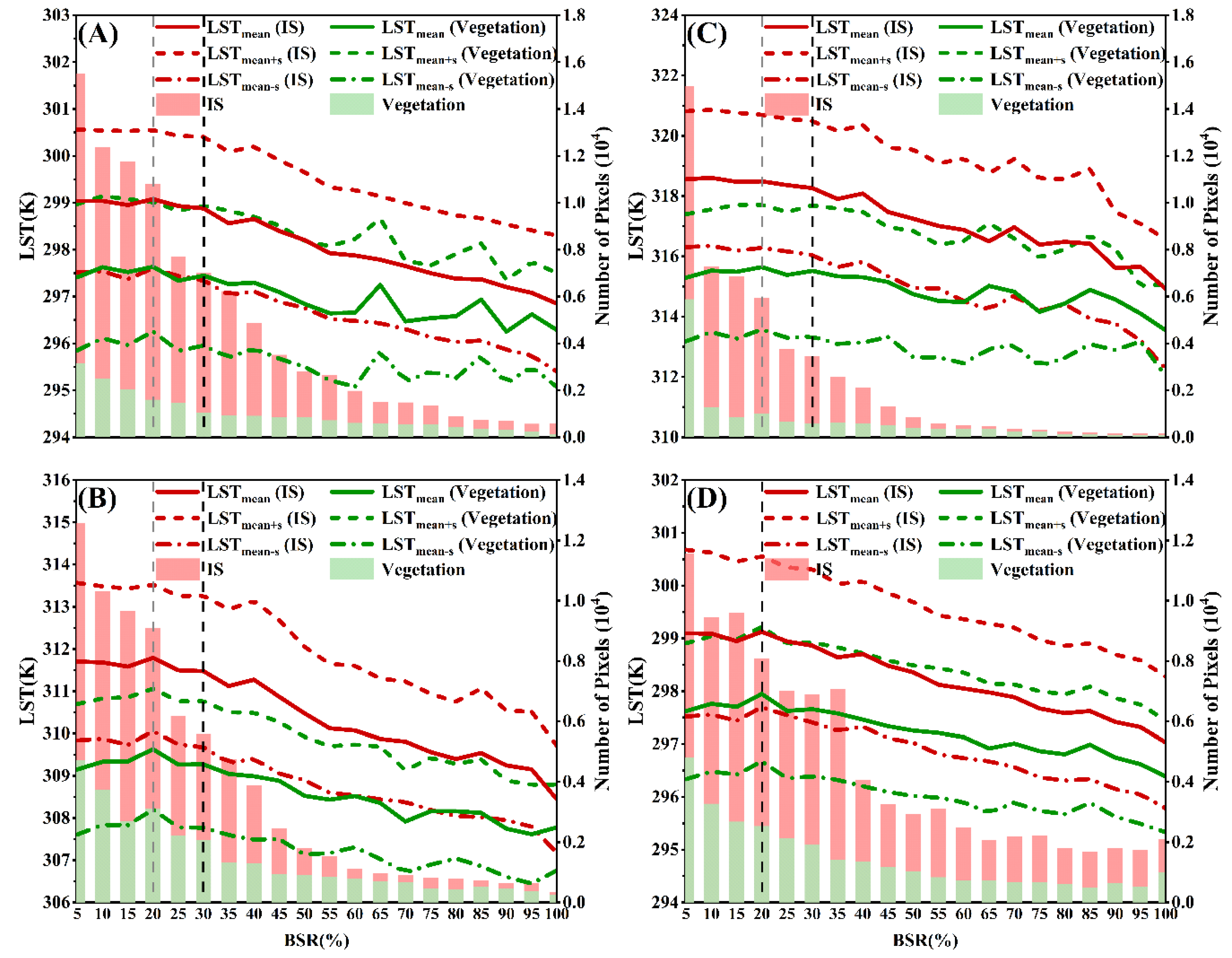
3.3.1. LST Mitigation of IS Pixels Totally Covered by BS

Quantitative evaluation of the cooling of BSs on the LST of pixels totally covered by IS (pure IS pixels) was carried out using Kriging interpolation (Section 2.3.5). IS pixels with a BSR of 100% were extracted to calculate the LST difference between BSs and simulated non-BSs surfaces (Figure 10). In general, the cooling effect of BSs on the LST lead to a decrease of 2.21 K (mean of 16 April and 7 May), 3.16 K (10 July), 1.98 K (28 September) and 1.24 K (mean of 14 and 25 December) at the satellite overpass time in different seasons, and these results are similar to that of previous studies [16]. For different regions, the mean cooling of BSs at the same time for the six dates was 1.59 K (in the second loop), 1.79 K (between the second and third loops), 1.96 K (between the third and fourth loops) and 1.85 K (between the fourth and fifth loops). The most significant impact of BSs on the LST was in the fourth loop on 10 July (3.67 K), and a weaker reduction of LST appeared in the second loop on 14 December (0.92 K). Additionally, the cooling of BSs in summer (10 July) reached a maximum, which was partially because the increased solar radiance in summer exposes IS to the sun with stronger amplitude of increasing LST, leading to the largest difference between BSs and non-BSs surfaces and illustrating the correctness of the interpolated results.

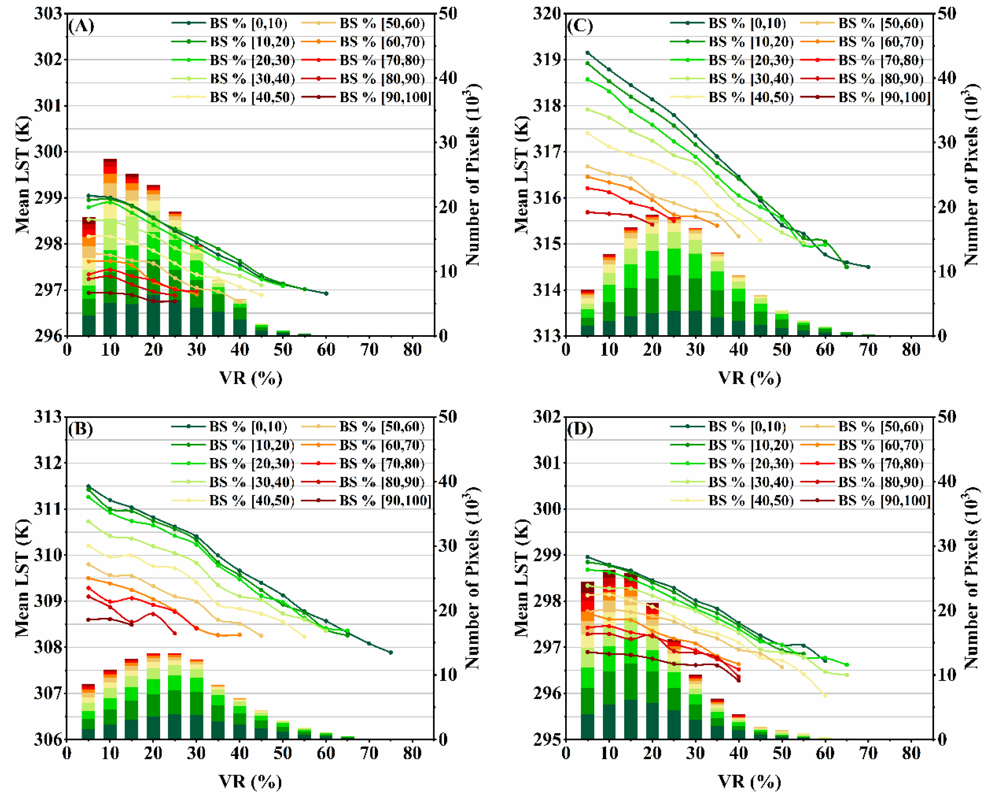
3.3.2. Cooling Variation of BSs with Changed BSR in Pure IS and Vegetation Pixels

To study how BSs affected the LST of IS and vegetation pixels under changes in the BSR, we counted the LST variation of these pixels with an increasing BSR and compared them. Since the lack of vegetation in winter might produce more complicated problems of mixed pixels, we only analyzed the cooling effect of BSs on 16 April and 7 May in spring, 10 July in summer and 28 September in autumn.
According to the principle of double the standard deviation, we removed outliers and integrated the entire LST dataset of IS and vegetation pixels in every season into 20 groups according to the BSR. Considering the anisotropy of the LST, we removed some data of factories in the fifth loop that might result in a more complicated thermal environment compared to that of the other loops (Section 2.3.4). Then, the mean LST of each group in every 5% interval was calculated and the results are shown in Figure 11, meanwhile, the relative number of pixels also be showed to ensure statistical meanings. To avoid the interference of non-BS surfaces, Figure 11 only illustrates the mean LST with a BSR from 5% to 100%. We observed a nonlinear relation between the BSR and mean LST for pure IS and vegetation pixels, and the correlations vary in different seasons.
The cooling effect of BSs on IS and vegetation pixels did not exceed 4 K for all seasons, which is similar to the results for IS pixels in Section 3.3.1. The most obvious change in LST was on 10 July in summer, which represented a more significant difference between BS and non-BS surfaces due to increased solar radiance, as explained in the previous section (Section 3.3.1). Notably, vegetation showed a warming process with pixels covered by more BSs when the BSR ranged from 5–20% in all datasets, as shown by the gray dotted lines in Figure 11 (covered by a black line on 28 September).
The cooling for IS and vegetation pixels had two stages of change in each dataset. For IS pixels, the effect of BSs could be ignored considering the errors from the LST retrieval when the BSR is small, which is emphasized by the black dotted lines in Figure 11. The same holds for vegetation, for which the mean cooling was −0.35 K (mean of 16 April and 7 May), −0.38 K (10 July) and −0.32 K (28 September). The number of pixels provided statistical meaning to the changed LST trend at different times; as shown by the histogram in Figure 11, which confirmed the reliability of the vegetation warming phenomenon, despite it being lower than the errors in the LST. The higher environmental LST of surrounding IS may have a more significant effect on vegetation than BSs through heat conduction when the BSR in pixels is small, especially on 10 July; hence, the LST of vegetation pixels gradually increased until reaching approximately 20% of the BSR [63].
The second stage was almost a linear change in which the LST of IS pixels evenly decreased to 2.52 K (mean of 16 April and 7 May), 3.63 K (on 10 July) and 2.01 K (on 28 September). For the vegetation pixels, the cooling amplitude at the same times were 1.25 K, 1.75 K and 1.15 K, thus showing a similar pattern to that of the IS pixels among the four data groups. Although the LST response of IS pixels to BSs on 28 September (20%, shown by a black dotted line) was faster than that on 16 April, 7 May and 10 July (30%), the BSs on 28 September exerted a weak effect on LST as shown in Figure 11, which was likely due to the lower environmental LST, and a small LST difference was observed between the BS and non-BS surfaces, thus decreasing the LST anisotropy [64]. The LST of pure IS pixels at four times are shown in Table 5.
We calculated the cooling effect of BSs for IS pixels using two methods in this paper, which unavoidably resulted in minor variations in the conclusions. For example, the LST decreased by 3.16 K and 3.63 K on 10 July using Kriging and statistics, respectively. The spatial heterogeneity of regional statistics result in the reliability of results is lower than that of the interpolation, which should consider the accuracy of LST retrieval. The statistical method is implemented to compare the relative cooling difference of BSs on vegetation and IS using the same method; the reason this method was utilized is explained above (Section 2.3.5). The similarity of the interpolated and statistical results showed that the statistics have high credibility in explaining the cooling effect of BSs.

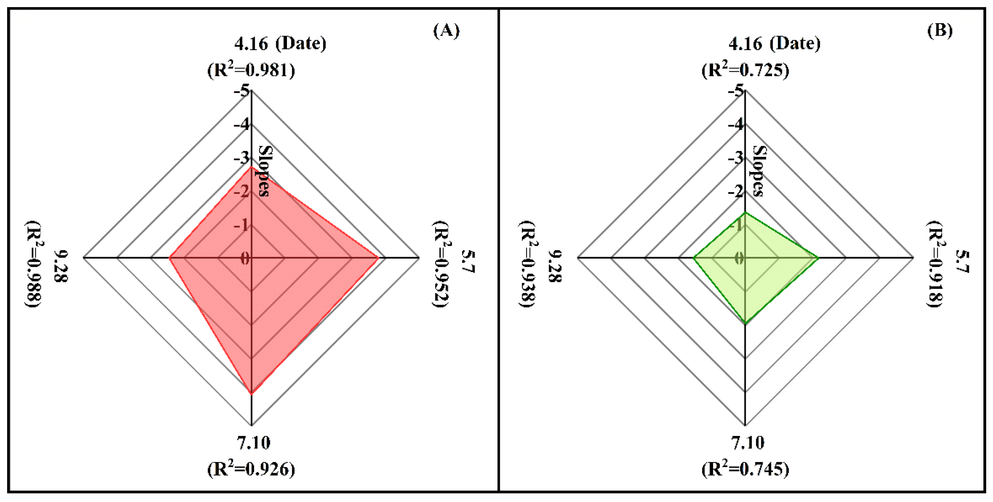
3.3.3. Sensitivity Analysis of BSs on LST of IS and Vegetation Pixels

A linear fitting was performed to assess the relations between the BSR (30–100% on 16 April, 7 May and 10 July, 20–100% on 28 September) and the mean LST; it showed that the temperature of IS pixels is more sensitive to BSs than vegetation pixels, which could be explained by two factors, as follows (Figure 12).
First, the slopes varied in all datasets, with a mean of −3.11 for IS pixels and −1.78 for vegetation (p < 0.05). Specifically, the former showed stronger sensitivity in three seasons, with slopes of −3.26 (mean of 16 April and 7 May), −3.71 (10 July) and −2.37 (28 September), whereas weaker LST variation occurred in the vegetation pixels at approximately −1.77, −2.04 and −1.53 for the same dates as the seasonal slopes, respectively (Figure 12). The mean of the former is almost twice as large as the latter, which is perhaps because the shading of buildings reduced the photosynthesis of vegetation and the thermal insulation of the vegetation suppresses the temperature decrease caused by the BSs [65]. As a result, weaker feedback occurred with vegetation pixels.
Second, the R2 values of the vegetation curves indicated strong instability and were not more than 0.8 on 16 April and 10 July. The urban vegetation pixels with a higher BSR may be surrounded by high-rise buildings; thus, the temperature of these pixels may increase due to the existence of the IS [55], which exceeded the cooling effect of BSs and vegetation. For example, Wetherly indicated an increase in IS cover of 10% results in 0.7 °C hotter pixels [63]. Hence, instability in the curve was observed, especially in the latter half, which represented building-intensive areas (Figure 11). IS pixels only showed a one-way cooling trend without self-regulation, which was superior to that of vegetation in terms of the stability of the curves. Hence, interference of IS might weaken the cooling effect of BSs on vegetation.
In addition, the reduction of the mean LST in IS pixels with an increasing BSR in all datasets had great seasonal volatility compared with that of the vegetation pixels. The values ranged from 2.01 K (28 September) to 3.63 K (10 July) for IS pixels (approximately 30–100%) and from 1.15 K (28 September) to 1.75 K (10 July) for vegetation pixels (20–100%). Theoretically, the change in the artificial IS temperature was entirely dependent on external factors, such as the solar radiance. As an independent living body, vegetation has its own internal regulation mechanism [66]. Since the ambient temperature varies with changed BSs, vegetation will maintain its own temperature by controlling transpiration [45]. Thus, vegetation inhibits the effect of BSs, and its temperature is not sensitive to the seasonal shadow change.
We also extracted the maximum and minimum in every BSR interval and investigated the sensitivity of LSTmax and LSTmin to IS and vegetation pixels with increasing BSR following the same method in Section 3.3.2. In general, the LSTmax of the two categories on four days all decreased with the BSR similar to the LSTmean, although a rising trend occurred for LSTmin, which was partially because the higher environmental LST covers the effect of BSs when the pixel temperature is relatively lower in urban regions.
Meanwhile, the LSTmin of IS and vegetation pixels all showed a weaker response to BSs than the LSTmax, suggesting that the lower temperature of these pixels are not sensitive to BSs cooling.

4. Discussion

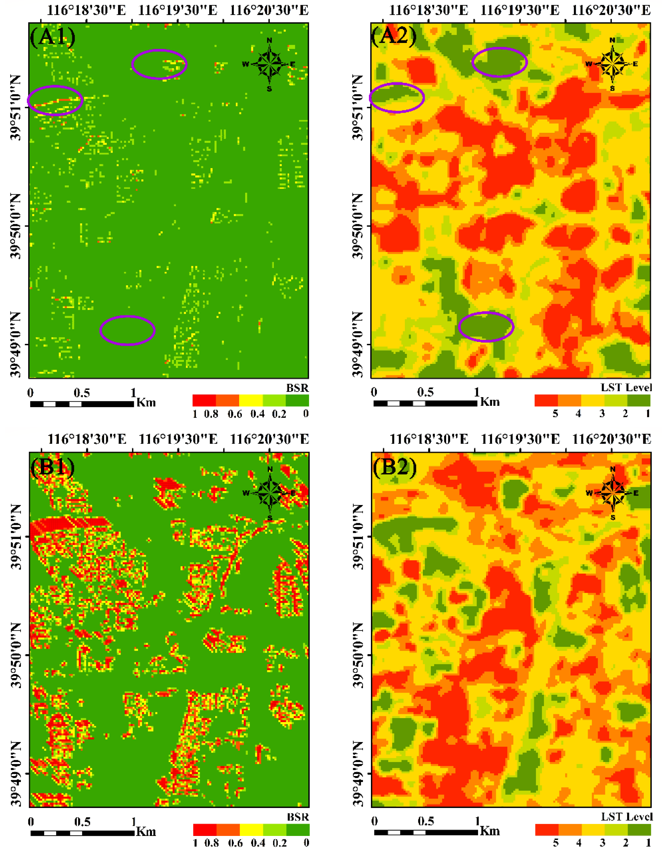
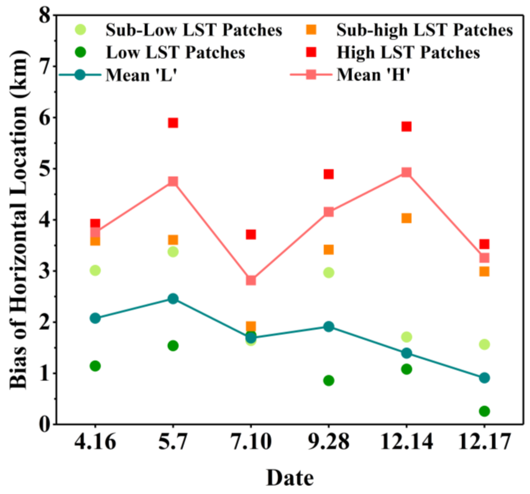
4.1. Relationship Between the Thermal Patch Centroid and BS

As an effective indicator describing spatial distribution, the thermal centroid could comprehensively describe the overall characteristics of thermal landscape distribution. Several scholars have indicated the spatiotemporal distribution of the thermal landscape in urban areas by analyzing the change of the thermal centroid [52]. Based on Section 3.2, we modeled the correlation between BSs and thermal landscape patches by calculating the distances of their centroids.
The centroids of five thermal landscape categories were obtained using LST-class data of pure IS pixels (Section 2.3.3). Because both shaded and nonshaded surfaces are included in medium LST patches of IS on different dates, which might not be conducive to an analysis of the seasonal effect of BSs on LST, we removed this class from the analysis. Figure 13 shows the temporal variation of the horizontal centroid location biases between BSs and thermal patches.
Among the five thermal categories, the centroid of the ‘L’ patches was closest to the BS centroid, with mean biases of 1.74 km for all datasets. This correlation was more obvious on 14 and 17 December, which demonstrated that the horizontal location of lower LST patch centroids was highly relevant to the distribution of BSs, and this was also confirmed by the conclusions in Section 3.2. In addition, area and number variation of ‘L’ patches were mainly controlled by BSs and showed significant seasonal characteristics with gradually increasing BSs, which is demonstrated by the bias of horizontal location in Figure 13. The bias of ‘H’ patches was relatively larger and did not show strong seasonal characteristics. A larger distance indicated a weaker effect of BSs on higher LST distribution.
Regrettably, the above study only focused on the influence of BSs on the LST distribution characteristics and ignored the analysis of changes in LST intensity. In Table 5, we calculated the LST discretization of IS pixels as shown by the standard deviation. What is the main reason for this seasonal change of LST discretization? Can the contribution of BSs be disregarded along with the thermal heterogeneity of building materials [58]? Previous studies have analyzed the centroids of UHI intensity using several methods, such as the Gaussian volume model, nonparametric fast Fourier transformation and mean-standard deviation [52]. Based on the above, the impact of BSs on LST intensity is worthy of a deeper analysis.

4.2. Effect of Adjacent Land Cover Types on BS Cooling at the Pixel Scale

As an important factor showing surface energy conditions, the LST derived from satellite remote sensing provides detailed spatial information about the complicated temperature distribution in urban environments with higher heterogeneity but unavoidably increases the uncertainty of LST retrievals due to the surface anisotropy and region smoothing of pixels [39,40,67]. A previous study shows that LST heterogeneity could reach 18 ℃ during the morning and 14 ℃ at night in the case of unmanned aerial vehicle (UAV)-thermal infrared (TIR) camera system. Satellite TIR sensors with higher resolution have similar difference, but not significant with lower resolution LST products such as that of MODIS [68].
The highest resolution of satellite TIR sensors is only approximately 100 m (90 m for ASTER, 100/120 m for Landsat-5/8, 60 m for Landsat-7), which is insufficient for analyzing urban thermal environments. Because of the 100 m (resampled to 30 m) spatial resolution of Landsat-8 LST data, the temperature of land cover types is largely influenced by the surrounding urban areas in a certain pixel. A study in Los Angeles in the USA comprehensively depicted the variation of LST with different combinations of features in subpixel scales, which could be neglected for the pixels’ LST, and it demonstrated that the daytime maximum anisotropic effects of LST can be up to 9 K for the most urbanized areas [63]. For instance, a pixel considered to be completely covered by vegetation might include IS, especially in regions with high building density. Thus, the influence of BSs in this pixel is not on vegetation, but on the mixed features [60]. In Figure 11, the increasing trend with the BSR from 5% to 20% for pure vegetation pixels suggested that the LST first increased due to the influence of IS and then was dominated by BSs. Consequently, the cooling effect might be heavily overestimated because of the differing sensitivity (IS and vegetation pixels) to BSs. Among them, we have no way to determine the proportion of temperature increase due to mixed pixels. Similarly, an IS pixel might include vegetation because of inevitable anisotropy based on the cooling of vegetation; hence, the effect of BSs is likely to be underestimated and excluding the effect of vegetation is difficult if higher resolution satellite remote sensing data are not available, not considering thermal camera onboard aircraft and UAV, which have meter-level spatial resolution but poor temporal continuity [69]. Note that even a pure pixel of IS might be influenced by the environmental LST of vegetation and the effect of BSs might produce uncertainty.
Hence, studies at the pixel scale may overlook the response of objects to BSs and the function of the environment surrounded cannot be ignored. The best solution to these problems is to develop technology for manufacturing better thermal infrared satellite sensors with higher spatial resolution because the current sensors do not satisfy the requirements for analysis. However, the fast, macro and uniform sampling of satellite remote sensing data is more conducive to spatiotemporal analyses than manual measurements [33]. In addition, the LST data from satellite remote sensing can provide more detailed spatial information about the cooling effect of BSs and insights into the spatial heterogeneity of LST caused by urban forms. As such, satellite remote sensing analyses are indispensable.

4.3. Influence of BSs on the Cooling Effect of Vegetation

Vegetation represents a potent tool for alleviating UHI [6,7,63]. Moreover, we showed that BSs also have a significant cooling effect. To ensure sufficient analytical data was obtained to mutually reinforce the effects of vegetation and BSs, pixels for which the sum of IS and vegetation proportion was greater than 0.9 were chosen from Section 2.3.4. Similarly, the BS data were used as indicator layers to determine the pixel selection condition (Section 2.3.5). According to Section 3.3.2, ten BS cover groups and the mean LST of each group in every 5% step of vegetation ratio (VR) increment were categorized and are shown in Figure 14. To avoid unrepresentative values due to small sample sizes, Figure 14 only illustrates the mean temperatures that are statistically meaningful and have more than 100 samples.
This conclusion about the relationship between the VR and mixed-pixel LST was consistent with previous research [7,63]; however, by regarding BSs as an indicator layer, we discovered that the cooling ability of vegetation has significant differences under changes in the BSR. With a higher BSR in pixels, the trend of LST variation is weaker under increases in VR, because the cooling process of vegetation via accelerated transpiration would be suppressed with less solar radiance [45], which would decrease the sensitivity of mixed-pixel LSTs to changes in vegetation. When the BSR exceeds 90%, the curves at four times gradually flatten (Figure 14).
Curves with a BSR less than and greater than 30% were relatively closer and farther from each other regardless of the proportion of vegetation changes, indicating that the cooling of BSs could be ignored under these circumstances, thus validating our conclusions in Section 3.3.2. Hence, under the influence of a variable BSR, the cooling of vegetation is restrained with higher VRs in pixels and represents manifestations of seasonal characteristics. Note that when both the BSR and VR ranged from 0 to 10%, the mixed-pixel LST decreased more if the VR reached 60% than that if the BSR ranged from 0 to 60%, which suggested the reduction of LST is more attributable to vegetation than BSs. Due to data limitations, we did not select the LST of 100% in the BSR and VR. In addition, the LST mitigation of mixed pixels with BSR from 0 to 60% was more than that in pure IS pixels (Section 3.3.2), indicating that the existence of vegetation promotes the cooling of BSs in IS pixels. Thus, the cooling of BSs might be overestimated if the pixel is mixed, which confirmed our previous opinions (Section 4.2). Based on our trial experiment, a deeper analysis must be performed to understand the cooling effect of BSs.

5. Conclusions

In this study, we explained the temporal effect of BSs on urban LST and mainly focused on the thermal landscape fragmentation and mitigation intensity of LST intensity under the influence of BSs. The results indicates that the distribution of IS LST in winter and the ability of IS and vegetation to mitigate intensity of LST in summer are strongly affected by BSs, while the cooling effect varies with different BSR in pixels. Furthermore, IS has greater sensitivity than vegetation LST.
However, our research has some shortcomings that we are currently unable to resolve. For example, previous research has shown that the accuracy of the geometric algorithm is lower than that of the spectral-based method [38]. However, due to the limitation of data sources and purpose of the research, geometric extraction was the most effective method despite the unavoidable uncertainty. Moreover, the resolution of Landsat-8 increases the proportion of mixed pixels in urban areas, as discussed in Section 4.1. Finally, our analysis of the cooling effect of BSs on pure IS pixels utilized regional pixel statistics in Section 3.3.2, which also inevitably introduced uncertainty due to the heterogeneity of the LST, especially in urban areas, for which we excluded some misclassified pixels in the fifth loop to reduce the LST volatility as much as possible. Although the feasibility of the statistical methods was indicated by a comparison with the interpolation method (Section 3.3.2), it is necessary to utilize other methods with higher accuracy, which could eliminate the LST heterogeneity to obtain better results in subsequent research.
The results in our study indicated that the LST distribution in winter was strongly affected by BS; hence, the influence of BSs on the seasonal change of the UHI centroid can be analyzed deeper. In addition, these works present limitations when conducted in single areas because of the difficulty applying the results to other cities with different climate in the future. Research on different urban forms, such as building densities and climatic environments, can also be compared to discuss the intensity of BSs under different conditions.

Author Contributions

Data curation, Y.C.; Formal analysis, K.Y.; Investigation, Z.C.; Methodology, D.W.; Project administration, Y.C.; Resources, A.G.; Writing—original draft, K.Y.; Writing—review & editing, J.L.

Funding

This work was supported by National Natural Science Foundation of China under Grants 41771448 and 41571342, Beijing Natural Science Foundation under Grant 8192025, Science and Technology Plans of Ministry of Housing and Urban-Rural Development of the People’s Republic of China and Opening Projects of Beijing Advanced Innovation Center for Future Urban Design, Beijing University of Civil Engineering and Architecture under Grants UDC2017030212 and UDC201650100, Project of State Key Laboratory of Earth Surface Processes and Resource Ecology under Grant 2017-ZY-03, and in part by Beijing Laboratory of Water Resources Security.

Conflicts of Interest

The authors declare no conflict of interest.

References

  1. Santamouris, M. Analyzing the heat island magnitude and characteristics in one hundred Asian and Australian cities and regions. Sci. Total Environ. 2015, 512, 582–598. [Google Scholar] [CrossRef] [PubMed]
  2. Voogt, J.A.; Oke, T.R. Thermal remote sensing of urban climates. Remote Sens. Environ. 2003, 86, 370–384. [Google Scholar] [CrossRef]
  3. Bowler, D.E.; Buyung-Ali, L.; Knight, T.M.; Pullin, A.S. Urban greening to cool towns and cities: A systematic review of the empirical evidence. Landscape Urban Plan. 2010, 97, 147–155. [Google Scholar] [CrossRef]
  4. Cai, Z.; Han, G.F.; Chen, M.C. Do water bodies play an important role in the relationship between urban form and land surface temperature? Sustain. Cities Soc. 2018, 39, 487–498. [Google Scholar] [CrossRef]
  5. Peng, J.; Jia, J.L.; Liu, Y.X.; Li, H.L.; Wu, J.S. Seasonal contrast of the dominant factors for spatial distribution of land surface temperature in urban areas. Remote Sens. Environ. 2018, 215, 255–267. [Google Scholar] [CrossRef]
  6. Hsieh, C.M.; Li, J.J.; Zhang, L.; Schwegler, B. Effects of tree shading and transpiration on building cooling energy use. Energy Build. 2018, 159, 382–397. [Google Scholar] [CrossRef]
  7. Zhou, W.; Wang, J.; Cadenasso, M.L. Effects of the spatial configuration of trees on urban heat mitigation: A comparative study. Remote Sens. Environ. 2017, 195, 1–12. [Google Scholar] [CrossRef]
  8. Bonafoni, S.; Keeratikasikorn, C. Land Surface Temperature and Urban Density: Multiyear Modeling and Relationship Analysis Using MODIS and Landsat Data. Remote Sens. 2018, 10, 1471. [Google Scholar] [CrossRef]
  9. Alobaydi, D.; Bakarman, M.A.; Obeidat, B. The Impact of Urban Form Configuration on the Urban Heat Island: The Case Study of Baghdad, Iraq. Procedia Eng. 2016, 145, 820–827. [Google Scholar] [CrossRef]
  10. Hendel, M.; Parison, S.; Grados, A.; Royon, L. Which pavement structures are best suited to limiting the UHI effect? A laboratory-scale study of Parisian pavement structures. Build. Environ. 2018, 144, 216–229. [Google Scholar] [CrossRef]
  11. Sun, Y.W.; Gao, C.; Li, J.L.; Li, W.F.; Ma, R.F. Examining urban thermal environment dynamics and relations to biophysical composition and configuration and socio-economic factors: A case study of the Shanghai metropolitan region. Sustain. Cities Soc. 2018, 40, 284–295. [Google Scholar] [CrossRef]
  12. Zhou, D.C.; Xiao, J.F.; Bonafoni, S.; Berger, C.; Deilami, K.; Zhou, Y.Y.; Frolking, S.; Yao, R.; Qiao, Z.; Sobrino, J.A. Satellite Remote Sensing of Surface Urban Heat Islands: Profress, Challenges, and Perspectives. Remote Sens. 2019, 11, 48. [Google Scholar] [CrossRef]
  13. Yin, C.H.; Yuan, M.; Lu, Y.P.; Huang, Y.P.; Liu, Y.F. Effects of urban form on the urban heat island effect based on spatial regression model. Sci. Total Environ. 2018, 634, 696–704. [Google Scholar] [CrossRef] [PubMed]
  14. Taleghani, M.; Kleerekoper, L.; Tenpierik, M.; Dobbelsteen, A.V.D. Outdoor thermal comfort within five different urban forms in The Netherlands. Build. Environ. 2015, 83, 65–78. [Google Scholar] [CrossRef]
  15. Lin, T.P.; Matzarakis, A.; Hwang, R.L. Shading effect on long-term outdoor thermal comfort. Build. Environ. 2010, 45, 213–221. [Google Scholar] [CrossRef]
  16. Ichinose, T.; Lei, L.; Lin, Y. Impacts of shading effect from nearby buildings on heating and cooling energy consumption in hot summer and cold winter zone of China. Energy Build. 2017, 136, 199–210. [Google Scholar] [CrossRef]
  17. Martinelli, L.; Lin, T.P.; Matzarakis, A. Assessment of the influence of daily shadings pattern on human thermal comfort and attendance in Rome during summer period. Build. Environ. 2015, 92, 30–38. [Google Scholar] [CrossRef]
  18. Villadiego, K.; Velay-Dabat, M.A. Outdoor thermal comfort in a hot and humid climate of Colombia: A field study in Barranquilla. Build. Environ. 2014, 75, 142–152. [Google Scholar] [CrossRef]
  19. Chun, B.; Guldmann, J.M. Impact of greening on the urban heat island: Seasonal variations and mitigation strategies. Comput. Environ. Urban 2018, 84, 1199–1209. [Google Scholar] [CrossRef]
  20. Akbari, H.; Kolokotsa, D. Three decades of urban heat islands and mitigation technologies research. Energy Build. 2016, 133, 834–842. [Google Scholar] [CrossRef]
  21. Li, D.H.W.; Wong, S.L. Daylighting and energy implications due to shading effects from nearby buildings. Appl. Energy 2007, 136, 199–210. [Google Scholar] [CrossRef]
  22. Shahidan, M.F.; Jones, P.J.; Gwilliam, J.; Salleh, E. An evaluation of outdoor and building environment cooling achieved through combination modification of trees with ground materials. Build. Environ. 2012, 58, 245–257. [Google Scholar] [CrossRef]
  23. Watanabe, S.; Nagano, K.; Ishii, J.; Horikoshi, T. Evaluation of outdoor thermal comfort in sunlight, building shade, and pergola shade during summer in a humid subtropical region. Build. Environ. 2014, 82, 556–565. [Google Scholar] [CrossRef]
  24. Hwang, R.L.; Lin, T.P.; Matzarakis, A. Seasonal effects of urban street shading on long-term outdoor thermal comfort. Build. Environ. 2011, 46, 863–870. [Google Scholar] [CrossRef]
  25. Johansson, E. Influence of urban geometry on outdoor thermal comfort in a hot dry climate: A studyin Fez, Morocco. Build. Environ. 2006, 41, 1326–1338. [Google Scholar] [CrossRef]
  26. Ali-Toudert, F.; Mayer, H. Numerical Study on the effects of aspect ratio and orientation on an urban street canyon on outdoor thermal comfort in hot and dry climate. Build. Environ. 2006, 41, 94–108. [Google Scholar] [CrossRef]
  27. Ali-Toudert, F.; Mayer, H. Thermal comfort in an east–west oriented street canyon in Freiburg (Germany) under hot summer conditions. Theor. Appl. Climatol. 2007, 87, 223–237. [Google Scholar] [CrossRef]
  28. Hamdi, R.; Schayes, G. Sensitivity study of the urban heat island intensity to urban characteristics. Int. J. Climatol. 2008, 28, 973–982. [Google Scholar] [CrossRef] [Green Version]
  29. Appelbaum, J.; Bany, J. Shadow effect of adjacent solar collectors in large scale systems. Sol. Energy 1979, 23, 497–507. [Google Scholar] [CrossRef]
  30. Ok, V. A procedure for calculating cooling load due to solar radiation: The shading effects from adjacent or nearby buildings. Energy Build. 1992, 19, 11–20. [Google Scholar] [CrossRef]
  31. Chan, A.L.S. Effect of adjacent shading on the thermal performance of residential buildings in a subtropical region. Appl. Energy 2012, 92, 516–522. [Google Scholar] [CrossRef]
  32. Lam, J.C. Shading effects due to nearby buildings and energy implications. Energy Convers. Manag. 2000, 41, 647–659. [Google Scholar] [CrossRef]
  33. Cao, X.; Onishi, A.; Chen, J.; Imura, H. Quantifying the cool island intensity of urban parks using ASTER and IKONOS data. Landsc. Urban Plan. 2010, 96, 224–231. [Google Scholar] [CrossRef]
  34. Dare, P.M. Shadow Analysis in High-Resolution Satellite Imagery of Urban Areas. Photogramm. Eng. Remote Sens. 2005, 71, 169–177. [Google Scholar] [CrossRef]
  35. Li, Y.Z.; Gong, X.Q.; Guo, Z.; Xu, K.P.; Hu, D.; Zhou, X.H. An index and approach for water extraction using Landsat–OLI data. Int. J. Remote Sens. 2016, 37, 3611–3635. [Google Scholar] [CrossRef]
  36. Chung, K.L.; Lin, Y.R.; Huang, Y.H.; Wang, L.J.; He, X.H. Efficient shadow detection of color aerial images based on successive thresholding scheme. IEEE Trans. Geosci. Remote Sens. 2009, 47, 671–682. [Google Scholar] [CrossRef]
  37. Liasis, G.; Stavrou, S. Satellite images analysis for shadow detection and building height estimation. ISPRS J. Photogramm. Remote Sens. 2016, 119, 437–450. [Google Scholar] [CrossRef]
  38. Hu, Y.F.; Zhang, Q.L. The Extraction of Building Shadow and the Estimation of Building Heights Based on Morphology and Spectral Characteristic Parameters. Bull. Surv. Mapp. 2018, 6, 22–26. [Google Scholar] [CrossRef]
  39. Hu, L.Q.; Monaghan, A.; Voogt, J.A.; Barlage, M. A first satellite-based observational assessment of urban thermal anisotropy. Remote Sens. Environ. 2016, 181, 111–121. [Google Scholar] [CrossRef] [Green Version]
  40. Lagouarde, J.P.; Hénon, A.; Irvine, M.; Voogt, J.; Pigeon, G.; Moreau, P.; Masson, V.; Mestayer, P. Experimental characterization and modelling of the nighttime directional anisotropy of thermal infrared measurements over an urban area: Case study of Toulouse (France). Remote Sens. Environ. 2012, 117, 19–33. [Google Scholar] [CrossRef]
  41. Degerickx, J.; Roberts, D.A.; Somers, B. Enhancing the performance of Multiple Endmember Spectral Mixture Analysis (MESMA) for urban land cover mapping using airborne lidar data and band selection. Remote Sens. Environ. 2019, 221, 260–273. [Google Scholar] [CrossRef]
  42. Fernández-Manso, A.; Quintano, C.; Roberts, D. Evaluation of potential of multiple endmember spectral mixture analysis (MESMA) for surface coal mining affected area mapping in different world forest ecosystems. Remote Sens. Environ. 2012, 127, 181–193. [Google Scholar] [CrossRef]
  43. Quintano, C.; Fernandez-Manso, A.; Roberts, D.A. Burn severity mapping from Landsat MESMA fraction images and Land Surface Temperature. Remote Sens. Environ. 2017, 190, 83–95. [Google Scholar] [CrossRef]
  44. Xiao, R.B.; Weng, Q.H.; Ouyang, Z.Y.; Li, W.F.; Schienke, E.W.; Zhang, Z.M. Land Surface Temperature Variation and Major Factors in Beijing, China. Photogramm. Eng. Remote Sens. 2008, 74, 451–461. [Google Scholar] [CrossRef]
  45. Du, H.Y.; Song, X.J.; Jiang, H.; Kan, Z.H.; Wang, Z.B.; Cai, Y.L. Research on the cooling island effects of water body: A case study of Shanghai, China. Ecol. Indic. 2016, 67, 31–38. [Google Scholar] [CrossRef]
  46. Yu, X.L.; Guo, X.L.; Wu, Z.C. Land Surface Temperature Retrieval from Landsat 8 TIRS—Comparison between Radiative Transfer Equation-Based Method, Split Window Algorithm and Single Channel Method. Remote Sens. 2014, 6, 9829–9852. [Google Scholar] [CrossRef] [Green Version]
  47. García-Santos, V.; Cuxart, J.; Martínez-Villagrasa, D.; Antònia Jiménez, M.; Simó, G. Comparison of Three Methods for Estimating Land Surface Temperature from Landsat 8-TIRS Sensor Data. Remote Sens. 2018, 10, 1450. [Google Scholar] [CrossRef]
  48. Chander, G.; Markham, B. Revised landsat-5 tm radiometric calibration procedures and postcalibration dynamic ranges. IEEE Trans. Geosci. Remote Sens. 2003, 41, 2674–2677. [Google Scholar] [CrossRef]
  49. Jaeger, J.A.G. Landscape division, splitting index, and effective mesh size: New measures of landscape fragmentation. Landsc. Ecol. 2000, 15, 115–130. [Google Scholar] [CrossRef]
  50. Han, B.L.; Liu, H.X.; Wang, R.S. Urban ecological security assessment for cities in the Beijing–Tianjin–Hebei metropolitan region based on fuzzy and entropy methods. Ecol. Model. 2015, 318, 217–225. [Google Scholar] [CrossRef] [Green Version]
  51. Peng, J.; Xie, P.; Liu, Y.X.; Ma, J. Urban thermal environment dynamics and associated landscape pattern factors: A case study in the Beijing metropolitan region. Remote Sens. Environ. 2016, 173, 145–155. [Google Scholar] [CrossRef]
  52. Quan, J.L.; Chen, Y.H.; Zhan, W.F.; Wang, J.F.; Voogt, J.; Wang, M.J. Multi-temporal trajectory of the urban heat island centroid in Beijing, China based on a Gaussian volume model. Remote Sens. Environ. 2014, 149, 33–46. [Google Scholar] [CrossRef]
  53. Raines, G.L. Description and comparison of geologic maps with FRAGSTATS-a spatial statistics program. Comput. Geosci. 2002, 28, 169–177. [Google Scholar] [CrossRef]
  54. Macdonald, D.W.; Bothwell, H.M.; Hearn, A.J.; Cheyne, S.M.; Haidir, I.; Hunter, L.T.B.; Kaszta, Z.; Linkie, M.; Macdonald, E.A.; Ross, J.; et al. Multi-scale habitat selection modeling identifies threats and conservation opportunities for the Sunda clouded leopard (Neofelisdiardi). Biol. Conserv. 2018, 227, 92–103. [Google Scholar] [CrossRef]
  55. Chen, X.; Wang, D.W.; Chen, J.; Wang, C.; Shen, M.G. The mixed pixel effect in land surface phenology: A simulation study. Remote Sens. Environ. 2018, 211, 338–344. [Google Scholar] [CrossRef]
  56. Li, X.M.; Chen, L.; Yang, M. A priori fully constrained least squares spectral unmixing based on sparsity. In Proceedings of the IEEE International Conference on Computer & Communications, Chengdu, China, 14–17 October 2016; IEEE Computer Society: Washington, DC, USA, 2016. [Google Scholar] [CrossRef]
  57. Xie, H.; Luo, X.; Xu, X.; Pan, H.Y.; Tong, X.H. Automated Subpixel Surface Water Mapping from Heterogeneous Urban Environments Using Landsat 8 OLI Imagery. Remote Sens. 2016, 8, 584. [Google Scholar] [CrossRef]
  58. Liu, W.Y.; Gong, A.D.; Zhou, J.; Zhan, W.F. Investigation on Relationships between Urban Building Materials and Land Surface Temperature through a Multi-resource Remote Sensing Approach. Remote Sens. Inf. 2011, 31, 46–53. [Google Scholar] [CrossRef]
  59. Wu, C.S.; Murray, A.T. Estimating impervious surface distribution by spectral mixture analysis. Remote Sens. Environ. 2003, 84, 493–505. [Google Scholar] [CrossRef]
  60. Chen, F.; Jiang, H.J.; Voorde, T.V.D. Land cover mapping in urban environments using hyperspectralAPEX data: A study case in Baden, Switzerland. Int. J. Appl. Earth Obs. 2018, 71, 70–82. [Google Scholar] [CrossRef]
  61. Graceline, J.S.; Pattabiraman, V. Improved pure pixel identification algorithms to determine the endmembers in hyperspectral images. Comput. Electr. Eng. 2018, 71, 515–532. [Google Scholar] [CrossRef]
  62. Svensson, M.K. Sky view factor analysis—Implications for urban air temperature differences. Meteorol. Appl. 2010, 11, 201–211. [Google Scholar] [CrossRef]
  63. Wetherley, E.B.; McFadden, J.P.; Roberts, D.A. Megacity-scale analysis of urban vegetation temperatures. Remote Sens. Environ. 2018, 213, 18–33. [Google Scholar] [CrossRef]
  64. Voogt, J.A. Assessment of an Urban Sensor View Model for thermal anisotropy. Remote Sen. Environ. 2008, 112, 482–495. [Google Scholar] [CrossRef]
  65. Vera, S.; Pinto, C.; Tabares-Velasco, P.C.; Bustamante, W.; Victorero, F.; Gironas, J.; Bonilla, C.A. Influence of Vegetation, Substrate, and Thermal Insulation of an Extensive Vegetated Roof on the Thermal Performance of Retail Stores in Semiarid and Marine Climates. Energy Build. 2017, 146, 312–321. [Google Scholar] [CrossRef]
  66. Catoni, R.; Gratani, L. Variations in leaf respiration and photosynthesis ratio in response to air temperature and water availability among Mediterranean evergreen species. J. Arid Environ. 2014, 102, 82–88. [Google Scholar] [CrossRef]
  67. Simó, G.; García-Santos, V.; Jiménez, M.A.; Martínez-Villagrasa, D.; Picos, R.; Caselles, V.; Cuxart, J. Landsat and Local Land Surface Temperature in a Heterogeneous Terrain Compared to MODIS Value. Remote Sens. 2016, 8, 849. [Google Scholar] [CrossRef]
  68. García-Santos, V.; Joan, C.; Jiménez, M.A.; Martínez-Villagrasa, D.; Simó, G.; Picos, R.; Caselles, V. Study of Temperature Heterogeneities at Sub-Kilometric Scales and Influence on Surface-Atmosphere Energy Interactions. IEEE Trans. Geosci. Remote 2018, 57, 640–654. [Google Scholar] [CrossRef]
  69. Niethammer, U.; James, M.R.; Rothmund, S.; Travelletti, J.; Joswig, M. UAV-based remote sensing of the Super-Sauze landslide: Evaluation and results. Eng. Geol. 2012, 128, 2–11. [Google Scholar] [CrossRef]
Figure 1. Location of the study area. (A) Map of China’s region. (B) Administrative planning and location of the study area. (C) Details of the study area. The background image is from Landsat-8 data on 10 July. The vector data are from the Chinese Academy of Sciences Resource and Environmental Science Data Center (http://www.resdc.cn/).
Remotesensing 11 00497 g001
Figure 2. Flow chart of the study. (A) Method flowchart for the study. (B) Details of the pure impervious surfaces (IS) and vegetation pixel extraction. (C) Details of the study of the building shadows (BS) cooling effect and its variation in pixels.
Remotesensing 11 00497 g002
Figure 3. Geometric structure of the sun-building sensor. Because the buildings in our study area are basically north-south oriented, we used this algorithm to extract building shadow (BS) pixels. (A) Shadow diagram of a single building, where ω is the angle between the north direction and the solar incident direction; S is the length of shadow on the ground, SN is the number of pixels occupied by the projection of S in the north direction, and H is the building height. (B) Actual shadow length under the mutual obstruction of buildings. SN1 is the shadow length with the influence of adjacent buildings; SN2 is the shadow length without the influence of adjacent buildings.
Remotesensing 11 00497 g003
Figure 4. Judgement of the actual SN (i,j). X, n, R, SN (i,j) and H(i,j) are the same as above; and β’ is the solar elevation in the north.
Remotesensing 11 00497 g004
Figure 5. Judgement of the building shadow (BS) pixels. ω has the same meaning as in Figure 3 and is correlated to the SAA. The red frames are BS pixels and the black ones are non-BS pixels.
Remotesensing 11 00497 g005
Figure 6. Six sample regions for analyzing the influence of building shadows (BS) on temperature discretization and fragmentation without vegetation in the study area. The background image is from Landsat-8 data on 10 July.
Remotesensing 11 00497 g006
Figure 7. Spatial distribution of building shadow (BS) pixels and land surface temperature (LST) patches on days of different seasons. (A1F1) Calculation of BSs with Formulas (1)–(4). (A2F2) Spatial distribution of LST. From (AF), the datasets represent 16 April and 10 May for spring, 10 July for summer, 28 September for autumn, 14 and 25 December for winter, respectively.
Remotesensing 11 00497 g007
Figure 8. Variation of the ratio of building shadows (BSR) in pixels and LST patches on 10 July (A1,A2) and 14 December (B1,B2). In (A1,B1), deeper red represents more building shadows (BS) in pixels (30 m) of Landsat-8 images, and deeper green indicates the opposite. In (A2,B2), the five LST classes are: ‘1’, low LST patches; ‘2’, sub-low LST patches; ‘3’, medium LST patches; ‘4’, sub-high LST patches; and ‘5’, high LST patches. The purple ellipses in (A1,A2) represent samples of urban cool islands (UCIs) formed by natural surfaces and BSs.
Remotesensing 11 00497 g008
Figure 9. Linear relationship between three indicators and the BSR in six regions of Figure 6. (AC) Percent of land (PLAND), ratio of patch number and patch density (PD), respectively. Circles and triangles are ‘H’ and ‘L’, respectively, and different colors express different seasons. Red solid and dashed lines show the fitting curves of ‘H’ and ‘L’, respectively.
Remotesensing 11 00497 g009
Figure 10. LST difference of pure IS pixels with building shadows (BS) and simulated non-BS surfaces. The reduction difference of the LST for six dates in different regions showed by (A), and for four regions at different dates in (B).
Remotesensing 11 00497 g010
Figure 11. The land surface temperature (LST) distribution (left-y-axis) versus the building shadow ratios (BSR) (x-axis with a 5% step) in different seasons with 16 April and 7 May for the spring case (A), (B), respectively; 10 July for the summer case (C); and 28 September for the autumn case (D). The red and green lines represent the LST for impervious surface (IS) and vegetation, respectively. The dotted lines are one standard deviation (s in the legend) from the mean LST. The corresponding colored bars (right y-axis) indicate the number of pixels for each land cover type in each BSR group. The black dashed vertical lines highlight the change of LST gradient for IS. The gray dashed vertical lines show that for vegetation (the two lines overlap with each other on 28 September.).
Remotesensing 11 00497 g011
Figure 12. Slopes of the fitting LST curves for the cooling effect of building shadows (BS) on days of different seasons. (A) For impervious surfaces (IS); and (B) for vegetation. R2 values in parentheses represent the goodness of fit of different datasets.
Remotesensing 11 00497 g012
Figure 13. Horizontal location biases between the centroids of the five thermal patch landscape categories and the centroids of building shadows (BSs) in six datasets. Squares and circles represent ‘H’ and ‘L’ patches, respectively, as defined in Section 3.2, and lines show the mean values of patches on different dates.
Remotesensing 11 00497 g013
Figure 14. Mean LST distribution (left-y-axis) versus the vegetation ratio (VR) (x-axis with a 5% step) at the satellite overpass time on 16 April (A), 7 May (B), 10 July (C) and 28 September (D). The colored solid lines represent the mean LST grouped into ten BS intervals. The corresponding colored bars (right y-axis) indicate the number of pixels in each VR group.
Remotesensing 11 00497 g014
Table 1. Satellite (Landsat-8) Images.
SensorDateTime (CST)Spatial Resolution (M)Solar Azimuth Angle (°)Solar Elevation Angle (°)
Landsat-825 December 201410:53100160.1123.64
Landsat-816 April 201510:52100143.0554.80
Landsat-814 December 201610:53100161.3524.14
Landsat-87 May 201710:52100138.1961.23
Landsat-810 July 201710:53100128.8164.47
Landsat-828 September 201710:53100154.9544.68
Table 2. Mean-standard deviation method for dividing LST classes.
Class of LSTDivision Interval of LST
High LSTT > M + S
Sub-high LSTM + 0.5 × S < T <= M + S
Medium LSTM − 0.5 × S < T <= M + 0.5 × S
Sub-low LSTM − S < T <= M − 0.5 × S
Low LSTT < M − S
M is the mean of LSTs and S is the standard deviation of LST.
Table 3. Metrics for the thermal landscape.
MetricFormula
PLANDPLAND = A i / A
A is the total area of landscape, A = i = 1 M A i ; Ai is the total area of landscape i (same as below); and M is the total number of landscape classes.
PDi PD i = N i / A i
PDi is the patch density of landscape i; and Ni is the number of landscape i.
Table 4. Pure pixel extraction results.
DatePure Pixels
VegetationIS
16 April 201537,887166,620
7 May 201783,635120,863
10 July 2017124,952100,513
28 September 2017105,556138,958
Table 5. Statistics of the LST discretization of IS pixels obtained by Landsat-8.
StatisticsMean (K)Std Dev 1 (K)
Date
16 April 2015310.3831.608
7 May 2017312.3012.327
10 July 2017318.7972.607
28 September 2017299.4291.782
1 Std Dev means standard deviation.

