Complex-Valued Convolutional Autoencoder and Spatial Pixel-Squares Refinement for Polarimetric SAR Image Classification

Abstract

Recently, deep learning models, such as autoencoder, deep belief network and convolutional autoencoder (CAE), have been widely applied on polarimetric synthetic aperture radar (PolSAR) image classification task. These algorithms, however, only consider the amplitude information of the pixels in PolSAR images failing to obtain adequate discriminative features. In this work, a complex-valued convolutional autoencoder network (CV-CAE) is proposed. CV-CAE extends the encoding and decoding of CAE to complex domain so that the phase information can be adopted. Benefiting from the advantages of the CAE, CV-CAE extract features from a tiny number of training datasets. To further boost the performance, we propose a novel post processing method called spatial pixel-squares refinement (SPF) for preliminary classification map. Specifically, the majority voting and difference-value methods are utilized to determine whether the pixel-squares (PixS) needs to be refined or not. Based on the blocky structure of land cover of PolSAR images, SPF refines the PixS simultaneously. Therefore, it is more productive than current methods worked on pixel level. The proposed algorithm is measured on three typical PolSAR datasets, and better or comparable accuracy is obtained compared with other state-of-the-art methods.

1. Introduction

Polarimetric synthetic aperture radar (PolSAR) image classification have been extensively used in topographic mapping, natural disaster monitoring, quantitative statistics on vegetation coverage, and urban and rural planning [1,2,3]. In recent years, deep learning models have been utilized to classify optical image and achieved superior accuracy [4]. Nevertheless, imaging mechanism of PolSAR images is different from that of the optical images [5]. These models achieve weak performance working on PolSAR images directly [6].

Before the deep learning models are applied to image classification, many traditional algorithms have been proposed. They focus on developing feature extractors and classifiers that are divided into two parts. The first part aims to design the filters associated with corresponding features. For example, wavelet transform filter is exploited to extract local features [7]. Markov random field and Fisher discriminant analysis are employed to learn spatial features between adjacent pixels [8,9]. In addition, Gabor wavelet filtering is used to extract texture and edge information in different directions [10]. 3D-Gabor filter is employed to generate multiple cubes for active learning [11]. The second part designs classifier via the obtained features to achieve classification tasks, including hierarchical classifier [12], wavelet transform classifier [13], and complex Wishart classifier [14]. Others such as k-nearest neighbor classifier used in [15], improve the classification accuracy significantly. Assisted by SVM and random forest classifier [16,17], Uhlmann et al. annotated PolSAR images according to color features and artificial designed features of PolSAR images [18]. These algorithms have shown better performance, but there is still a need to design hand crafted feature extractors and select suitable classifiers based on experiences that not only spends much time on designing models but also produces poor generalization performance.

With the significant breakthrough of convolutional neural network (CNN), it has performed in optical image classification task [19]. Deep learning methods are introduced in PolSAR images classification. For example, Zhang et al. exploited stack sparse autoencoder to extract spatial sparse features, reducing the effect of speckle noise on pixel level [20]. Geng et al. applied deep recurrent encoding neural networks (DRENNs) to extract contextual information of SAR images [21]. In [22], stack autoencoder is utilized to extract PolSAR features from synthetic target database firstly. Then the classifier, which is constructed of multi-layer perceptron network, is used to label the urban area. Nonetheless, in these models, adequate training datasets are required to achieve high classification accuracy. However, attaining sufficient training samples is difficult because of the rarity and confidentiality of remote sensing images. Consequently, Shang et al. added an information encoder to CNN to increase samples’ utilization [23]. Gao et al. obtained joint feature map using CNN and Multiple Feature Learning to increase the discriminant performance of the features [24]. There are also many unsupervised feature extraction methods, such as sparse autoencoder (SAE) [25], convolutional autoencoder (CAE) [26], multilayer autoencoder with a restriction using Euclidean distance [27], discriminant Analysis with Graph Learning (DAGL) [28], multilayer autoencoders and self-paced learning (SPL) [29], Wishart autoencoder (WAE) and Wishart convolutional autoencoder (WCAE) [30], and Wishart deep belief network (W-DBN) [31]. Specifically, the prior information of Wishart distribution of PolSAR data are used in WAE and WCAE, which increase the accuracy rate by over 2%. W-DBN is composed of the Wishart-Bernoulli restricted Boltzmann machine (WBRBM), achieving better classification performance based on unsupervised pre-training and fine tuning. However, only the real value of coherence matrix or covariance matrix of pixels of PolSAR images is used among these algorithms. To solve this problem, Zhang et al. introduced phase information to CNN and proposed a complex-valued CNN (CV-CNN) [6], which had achieved comparable accuracy and verified the significance of phase information in PolSAR image. But massive annotated training datasets are needed in CV-CNN.

To alleviate the problem that CAE cannot extract the features of PolSAR image adequately with tiny amounts of training datasets, complex-valued convolutional autoencoder network (CV-CAE) is proposed in this paper. Firstly, CV-CAE extracts features from unannotated complex-valued input patch, then training complex-valued fully connected network (CFC) and fine tune CV-CAE with annotated training data. Experiments with three typical datasets show that the classification accuracy can be further improved. Nowadays, many post processing methods have been introduced into the PolSAR image classification. Among them, Liu et al. proposed the Cleaning algorithm, in which Bayesian theory and local spatial information are employed to rectify the class of each pixel [31]. In [32], refined spatial-anchor graph is proposed to reassign the border pixels using majority voting and distance measurement. These methods increase the classification accuracy by refining the pixels one by one. Therefore, Considering the efficiency of postprocessing methods, SPF is proposed in this paper by calculating blocky land cover structure of preliminary classified map. SPF uses majority voting and difference-value to determine whether the refined condition is met or not, and then refines the class of all pixels within the PixS. Therefore, compared with pixel level refinement, SPF can obtain higher refinement efficiency. The proposed algorithm is evaluated using three PolSAR datasets, and achieve better accuracy than other compared algorithms.

The rest of this paper is strctured as follows. Section 2 describes the framework of proposed CV-CAE and SPF in details. Data preprocessing and experimental analysis are introduced in Section 3. The conclusion is discussed in Section 4.

2. Classification Based on CV-CAE Network

In our work, considering the phase and amplitude information of PolSAR images. CV-CAE network is proposed by extending the unsupervised model CAE to complex domain. In order to promote the efficiency of pixel level refinement, a post processing method, SPF, is adopted. The architecture and the training process of CV-CAE, along with the implementation method of SPF are outlined in the following.

2.1. The Framework of the Proposed Algorithm

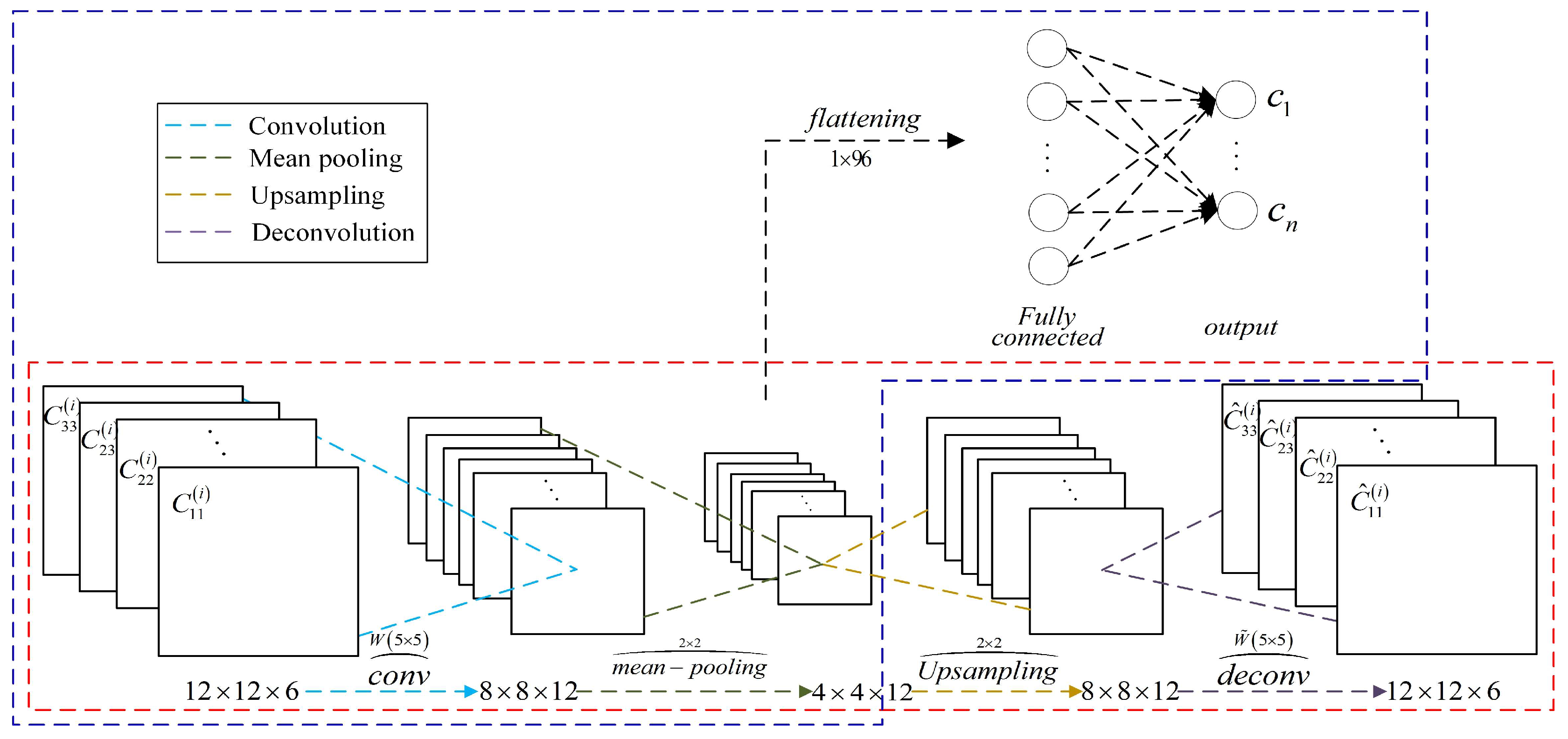
The framework of CV-CAE, depicted in Figure 1, consists of the feature extraction and classification. Which are marked with the red and blue dotted box respectively. Detailed explanation is as follows. Firstly, the network in red box extracts features. Then classification network that formed with encode part of CV-CAE after training and the CFC achieves classification task. Where $C_{11}^{\left(i\right)}$ is the first channel value of each pixel in the ith input patch, ${\widehat{C}}_{11}^{\left(i\right)}$ is the decoding value of $C_{11}^{\left(i\right)}$, $c_n$ is the nth value of classification result, and n indicates the number of terrain type.

2.1.1. CV-CAE

CV-CAE consists of four complex-valued parts, which are input, output, encoding, and decoding. The configuration of CV-CAE is given in

Table 1. The Framework and Parameters Configuration of CV-CAE.

Layer NO.	Architecture	Output Size (Pixels)
1	Input layer	12 × 12 × 6
2	Conv.12 (5 × 5 × 6)/sigmoid	8 × 8 × 12
3	Mean-Po.2 (2 × 2)	4 × 4 × 12
4	Upsampl.2 (2 × 2)	8 × 8 × 12
5	Deconv.6 (5 × 5 × 12)/sigmoid	12 × 12 × 6
6	Fully connected	1 × N

. The encoding includes convolution and mean pooling corresponding to the second and third layer. Next two layers, upsampling and deconvolution, are the components of decoding. Sigmoid activation function is utilized in CV-CAE.

In Table 1, the structure and parameters of convolutional layer and mean pooling layer are represented by “Conv. feature mappings number (kernel size)/activation function” and “Mean-Po. Stride (pooling size)”. In addition, the structure and parameters of the next two layers are similar to those of the two layers. Classification network is formed with Fully connected layer. Output size is the number of output feature mapping. N is the number of terrain type.

Spatial features play a pivotal role in classification of PolSAR images. Therefore, input of CV-CAE is a complex-valued patch that cropped from original PolSAR images. As shown in Figure 1, $C_{11}^{\left(i\right)},C_{12}^{\left(i\right)},C_{13,}^{\left(i\right)},C_{22}^{\left(i\right)},C_{23,}^{\left(i\right)}$ and $C_{33}^{\left(i\right)}$ are complex-valued pixel values of six channels in the $ith$ input patch. Considering the terrain type of PolSAR images [33,34], the size of $12\times 12$ is selected as input patch. On the one hand, this size is big enough to contain the spatial feature that is needed for classification. On the other hand, with the smaller input size, the computational efficiency is increased and the risk of over-fitting is prevented [23].

In encoding part, complex-valued convolution extracts discriminant features for classification task from the complex-valued input patch. They are different from that of real-valued convolution for these features include spatial and polarized information. All parameters in complex-valued convolutional operation are complex value. Specifically, the $ith$ complex input patch is $X_{ic}^{\left(l\right)}\in {}^{W_1\times H_1\times C}$, where l is the layers’ number, and c is the number of channels ($c=1,2,···,C$). The output corresponding to the $ith$ input is $y_{ik}^{\left(l\right)}\in {}^{W_Y\times H_Y\times K}$, k is the number of feature mappings. The complex-valued convolution is defined as

$$\begin{array}{c}{y}_{ik}^{\left(l\right)}={\displaystyle \sum _{c=1}^C}{X}_{ic}^{\left(l\right)}\ast W_{ik}^{\left(l\right)}+b_k^{\left(l\right)}\hfill \\ ={\displaystyle \sum _{c=1}^C}\left(real\left(X_{ic}^{\left(l\right)}\right)·real\left(W_{ik}^{\left(l\right)}\right)-imag\left(X_{ic}^{\left(l\right)}\right)·imag\left(W_{ik}^{\left(l\right)}\right)\right)\hfill \\ +j{\displaystyle \sum _{c=1}^C}\left(real\left(X_{ic}^{\left(l\right)}\right)·imag\left(W_{ik}^{\left(l\right)}\right)+imag\left(X_{ic}^{\left(l\right)}\right)·real\left(W_{ik}^{\left(l\right)}\right)\right)\hfill \\ +b_k^{\left(l\right)}\hfill \end{array}$$

(1)

where $real\left(·\right)$ and $imag\left(·\right)$ are real and imaginary part of the complex value ·. Character * represents convolutional operation. $W_{ik}^{\left(l\right)}$ is the convolutional kernel of size $W_2\times H_2\times C\times K$. Generally, kernels with size of $3\times 3$ or $5\times 5$ are recommended because they are more effective in feature extraction than others [35,36]. $b_k^{\left(l\right)}$ is bias. The parameters of CV-CAE to be trained in the $lth$ layer of convolutional operation are $W_{ik}^{\left(l\right)}$ and $b_k^{\left(l\right)}$. In complex domain, whose number is two times that of the real field. That is $2\times \left(W_2\times H_2\times C\times K+K\right)$. For a convolutional operation with stride S and zero-padding P, the size of feature mappings of convolution result is calculated by

$$\begin{array}{c}{W}_Y=\left(W_1-W_2+2P\right)/S+1\hfill \\ H_Y=\left(H_1-H_2+2P\right)/S+1\hfill \end{array}$$

(2)

In Equation (1), only linear transformation is performed on the input data. In order to obtain improved generalization and robustness of CV-CAE, nonlinear operations must be adopted. In neural networks, sigmoid and ReLU are the two commonly recommended [37]. In addition, they showed good performance on nonlinear transformation and accelerated the speed of training. In CV-CAE, the complex-valued nonlinear operation is defined as

$$Y_{ik}^{\left(l\right)}=\sigma \left(real\left(y_{ik}^{\left(l\right)}\right)\right)+j\sigma \left(imag\left(y_{ik}^{\left(l\right)}\right)\right)$$

(3)

where $\sigma \left(z\right)=\frac{1}{1+e^{-z}}$ denotes sigmoid activation function. $Y_{ik}^{\left(l\right)}$, the size same as $y_{ik}^{\left(l\right)}$, is the result of complex-valued nonlinear transformation.

Pooling is reducing the dimension of its input features based on similarity, which not change the number of channels at all. By means of pooling, the pivotal features are preserved and the redundant information is reduced. Therefore, the calculation and convergence of networks are more efficient. In neural networks, the most useful pooling operations are max-pooling and mean-pooling. Pooling size and stride are dominant parameters. Appropriate parameter values not only eliminate redundant information but also retain the discriminant features. Based on the previous experience, the pooling size $2\times 2$ or $3\times 3$ and stride 2 are commonly recommended.

No padding convolution with kernel size 5 and stride 1 is employed in encoding part. The number of convolutional kernels is 12. In the complex domain, max pooling cannot be directly adopted. So the mean pooling with a pooling size 2 and a stride 2 is exploited in CV-CAE. According to Equation (2), with the complex-valued input patch size of $12\times 12\times 6$, the size of feature mappings after convolution and mean pooling operation are $8\times 8\times 12$ and $4\times 4\times 12$.

Decoding part consists of uppooling and deconvolution, and it is the inverse process of encoding, which aims to reconstruct the input of encoding. In uppooling, feature mappings of encoding are extended by utilizing the location information retained in the pooling process. There are different extension methods with diverse pooling operation. For inverse mean pooling, the result is the case that a pixel value in the feature maps is copied to all positions within the pooling size. Deconvolution, also called transposition convolution, is the inverse process of convolution. In deconvolution, the sparse image representation generated by uppooling is reconstructed to the identical resolution as input patch of encoding. Deconvolution result ${\tilde{Y}}_{ic}^{\left(l\right)}$ is calculated by

$${\tilde{Y}}_{ic}^{\left(l\right)}=\sigma \left(real\left({\tilde{y}}_{ic}^{\left(l\right)}\right)\right)+j\sigma \left(imag\left({\tilde{y}}_{ic}^{\left(l\right)}\right)\right)$$

(4)

$$\begin{array}{c}{\tilde{y}}_{ic}^{\left(l\right)}={\displaystyle \sum _{k=1}^K}{Y}_{ik}^{\left(l\right)}\ast {\tilde{W}}_{ic}^{\left(l\right)}+{\tilde{b}}_c^{\left(l\right)}\hfill \\ ={\displaystyle \sum _{k=1}^K}\left(real\left(Y_{ik}^{\left(l\right)}\right)·real\left({\tilde{W}}_{ic}^{\left(l\right)}\right)-imag\left(Y_{ik}^{\left(l\right)}\right)·imag\left({\tilde{W}}_{ic}^{\left(l\right)}\right)\right)\hfill \\ +j{\displaystyle \sum _{k=1}^K}\left(real\left(Y_{ik}^{\left(l\right)}\right)·imag\left({\tilde{W}}_{ic}^{\left(l\right)}\right)+imag\left(Y_{ik}^{\left(l\right)}\right)·real\left({\tilde{W}}_{ic}^{\left(l\right)}\right)\right)\hfill \\ +{\tilde{b}}_c^{\left(l\right)}\hfill \end{array}$$

(5)

The parameters to be trained in deconvolution are ${\tilde{W}}_{ic}^{\left(l\right)}$ and ${\tilde{b}}_c^{\left(l\right)}$. Where ${\tilde{W}}_{ic}^{\left(l\right)}$ is the deconvolution kernel with size $W_2\times H_2\times K\times C$. The number of parameters is $2\times \left(W_2\times H_2\times K\times C+C\right)$, C is the number of bias ${\tilde{b}}_c^{\left(l\right)}$. In decoding part, the input features of the uppooling are also the feature mappings of encoding. The size of which is $4\times 4\times 12$. The output of uppooling with size of $8\times 8\times 12$. Kernels size $5\times 5$ and the number of output features 6 are employed in deconvolution. Therefore, the output size of decoding is $12\times 12\times 6$.

2.1.2. Classification Network

Encoding of CV-CAE after training and CFC are included in the classification network. Encoding part has been elaborated in Section 2.1.1 and will not be repeated here. The input of CFC ${\stackrel{\rightharpoonup }{Y}}_{ik}^{\left(l\right)}$ is a vector that is obtained by reshaping encoding result ${\tilde{Y}}_{ic}^{\left(l\right)}$. The number of input neurons is equal to the number of the elements in this vector. The result of CFC is $O_{in}^{\left(l\right)}$, n is the number of neurons in a complex-valued output layer (n = 1, 2, ⋯, N), which is also the number of terrain type of PolSAR images. Therefore, $O_{in}^{\left(l\right)}$ can be described as

$$\begin{array}{c}\hfill O_{in}^{\left(l\right)}=\sigma \left(real\left(o_{in}^{\left(l\right)}\right)\right)+j\sigma \left(imag\left(o_{in}^{\left(l\right)}\right)\right)\end{array}$$

(6)

$$\begin{array}{c}\hfill o_{in}^{\left(l\right)}=\sum _{k=1}^K{\stackrel{\rightharpoonup }{Y}}_{ik}^{\left(l\right)}·{W_{in}^{\prime }}^{\left(l\right)}+{b_n^{\prime }}^{\left(l\right)}\end{array}$$

(7)

where character · represents dot product operation. The parameters to be trained are weights ${W_{in}^{\prime }}^{\left(l\right)}$ and bias ${b_n^{\prime }}^{\left(l\right)}$. In CFC, the number of input elements are $4\times 4\times 12$. And the number of bias ${b_n^{\prime }}^{\left(l\right)}$ is the neurons N of output layer. N is varied in different datasets.

2.2. Network Training

In CV-CAE, there are two stages of training. Firstly, unannotated datasets are utilized to train CV-CAE. The encoding of CV-CAE after training is employed to extract features. Then, annotated dataset are applied to train the CFC and fine tune the encoding part. The detailed procedure is as follows.

2.2.1. CV-CAE Training

The training of CV-CAE is to minimize the loss function $J\left(\theta \right)$, which aims to reconstruct the input of CV-CAE by optimizing the parameters $\theta$. $\theta$ includes convolutional kernel $W_{ik}^{\left(l\right)}$, ${\tilde{W}}_{ic}^{\left(l\right)}$ and bias $b_k^{\left(l\right)}$, ${\tilde{b}}_c^{\left(l\right)}$. In CV-CAE, the reconstruction error $J\left(\theta \right)$ with input $X_{ic}^{\left(l\right)}$ and output ${\tilde{Y}}_{ic}^{\left(l\right)}$ can be calculated by

$$J\left(\theta \right)=\frac{1}{2N}\sum _{i=1}^N\left[{∥real\left({\tilde{Y}}_{ic}^{\left(l\right)}\right)-real\left(X_{ic}^{\left(l\right)}\right)∥}^2+{∥imag\left({\tilde{Y}}_{ic}^{\left(l\right)}\right)-imag\left(X_{ic}^{\left(l\right)}\right)∥}^2\right]$$

(8)

where $l=1,2,···,L$ and $c=1,2,···C$ represent network layers and channel numbers respectively. The ${\tilde{W}}_{ic}^{\left(l\right)}$ and ${\tilde{b}}_c^{\left(l\right)}$ in decoding can be updated iteratively using the following Equations.

$${\tilde{W}}_{ic}^{\left(l\right)}={\tilde{W}}_{ic}^{\left(l\right)}-\eta \frac{\partial J\left(\theta \right)}{\partial {\tilde{W}}_{ic}^{\left(l\right)}}$$

(9)

$${\tilde{b}}_c^{\left(l\right)}={\tilde{b}}_c^{\left(l\right)}-\eta \frac{\partial J\left(\theta \right)}{\partial {\tilde{b}}_c^{\left(l\right)}}$$

(10)

As can be known from Equation (8), $J\left(\theta \right)$ is a function of parameter $\theta$. To solve Equations (9) and (10), finding the partial derivatives $\partial J\left(\theta \right)/\phantom{J\left(\theta \right)\partial {\tilde{W}}_{ic}^{\left(l\right)}}\partial {\tilde{W}}_{ic}^{\left(l\right)}$ and $\partial J\left(\theta \right)/\phantom{\partial J\left(\theta \right)\partial {\tilde{b}}_c^{\left(l\right)}}\partial {\tilde{b}}_c^{\left(l\right)}$ are needed. By imitating the real-valued solution process and extending the chain rule to the complex domain, the result can be defined as

$$\begin{array}{c}\frac{\partial J\left(\theta \right)}{\partial {\tilde{W}}_{ic}^{\left(l\right)}}=\frac{\partial J\left(\theta \right)}{\partial real\left({\tilde{W}}_{ic}^{\left(l\right)}\right)}+\frac{\partial J\left(\theta \right)}{\partial imag\left({\tilde{W}}_{ic}^{\left(l\right)}\right)}\hfill \\ =\left(\frac{\partial J\left(\theta \right)}{\partial real\left({\tilde{Y}}_{ic}^{\left(l\right)}\right)}\frac{\partial real\left({\tilde{Y}}_{ic}^{\left(l\right)}\right)}{\partial real\left({\tilde{W}}_{ic}^{\left(l\right)}\right)}+\frac{\partial J\left(\theta \right)}{\partial imag\left({\tilde{Y}}_{ic}^{\left(l\right)}\right)}\frac{\partial imag\left({\tilde{Y}}_{ic}^{\left(l\right)}\right)}{\partial real\left({\tilde{W}}_{ic}^{\left(l\right)}\right)}\right)\hfill \\ +j\left(\frac{\partial J\left(\theta \right)}{\partial real\left({\tilde{Y}}_{ic}^{\left(l\right)}\right)}\frac{\partial real\left({\tilde{Y}}_{ic}^{\left(l\right)}\right)}{\partial imag\left({\tilde{W}}_{ic}^{\left(l\right)}\right)}+\frac{\partial J\left(\theta \right)}{\partial imag\left({\tilde{Y}}_{ic}^{\left(l\right)}\right)}\frac{\partial imag\left({\tilde{Y}}_{ic}^{\left(l\right)}\right)}{\partial imag\left({\tilde{W}}_{ic}^{\left(l\right)}\right)}\right)\hfill \end{array}$$

(11)

with Equations (6)–(8), the second and third term in Equation (11) are zero. So there are two terms in Equation (11). The result can be calculated by utilizing same methods in bias ${\tilde{b}}_c^{\left(l\right)}$

$$\begin{array}{c}\frac{\partial J\left(\theta \right)}{\partial {\tilde{b}}_c^{\left(l\right)}}=\frac{\partial J\left(\theta \right)}{\partial real\left({\tilde{b}}_c^{\left(l\right)}\right)}+\frac{\partial J\left(\theta \right)}{\partial imag\left({\tilde{b}}_c^{\left(l\right)}\right)}\hfill \\ =\frac{\partial J\left(\theta \right)}{\partial real\left({\tilde{Y}}_{ic}^{\left(l\right)}\right)}\frac{\partial real\left({\tilde{Y}}_{ic}^{\left(l\right)}\right)}{\partial real\left({\tilde{b}}_c^{\left(l\right)}\right)}+j\frac{\partial J\left(\theta \right)}{\partial imag\left({\tilde{Y}}_{ic}^{\left(l\right)}\right)}\frac{\partial imag\left({\tilde{Y}}_{ic}^{\left(l\right)}\right)}{\partial imag\left({\tilde{b}}_c^{\left(l\right)}\right)}\hfill \end{array}$$

(12)

The same update method is exploited as in encoding. After training with unannotated dataset, the discriminant features that obtained by encoding part of CV-CAE are used as input for CFC.

2.2.2. Classification Network Training

Annotated dataset are applied to train the CFC in this section. In real-valued convolutional autoencoder (RV-CAE), softmax is used as output layer to obtain the probability of each category. However, complex-valued input data cannot attain the certain probabilistic value of every class. Therefore, the output layer is a complex-valued fully connected layer with N neurons. Mean square error (MSE) between the output of the CFC and the one-hot vector are used as loss function. In complex domain, ON value of one-hot vector is recorded as $1+j$, others are 0. The length of vector is the number of classes of the datasets. Therefore, the loss function of CFC is defined as

$$E=\frac{1}{2N}\sum _{i=1}^N\left[{\left(real\left(T_i\right)-real\left(O_{in}^{\left(l\right)}\right)\right)}^2+{\left(imag\left(T_i\right)-iamg\left(O_{in}^{\left(l\right)}\right)\right)}^2\right]$$

(13)

where $O_{in}^{\left(l\right)}$ is the result of CFC, and $T_i$ is the target corresponding to the input of $O_{in}^{\left(l\right)}$. In this part, the updating method of complex-valued weight ${W_{in}^{\prime }}^{\left(l\right)}$ and bias ${b_n^{\prime }}^{\left(l\right)}$ are similar with those in encoding of CV-CAE.

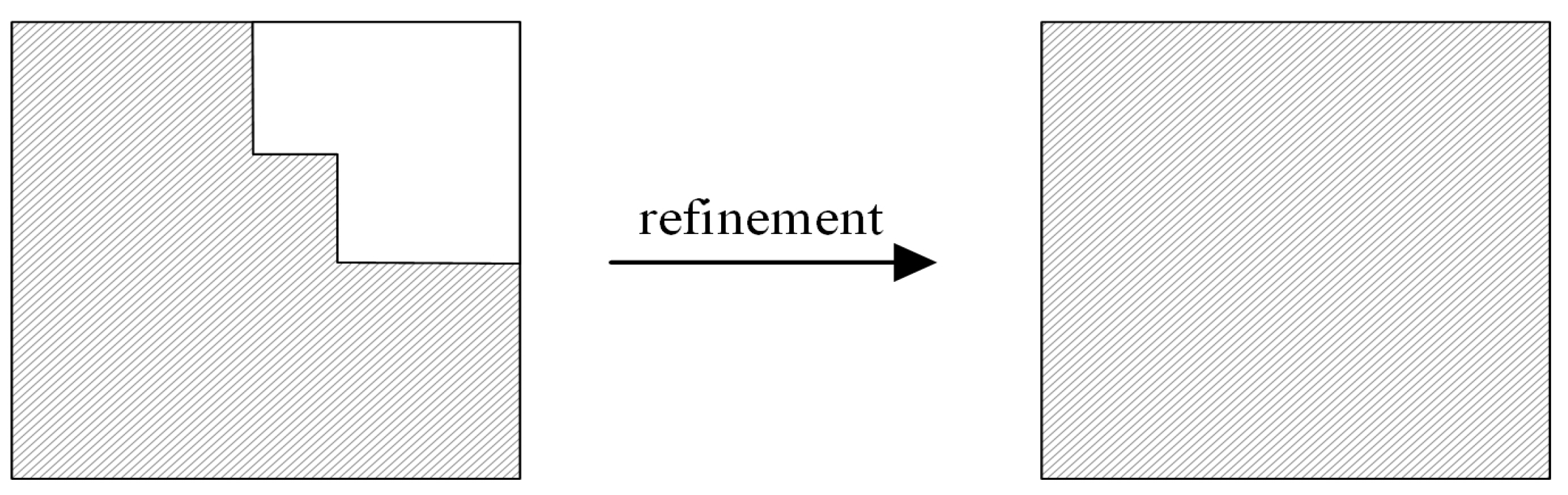
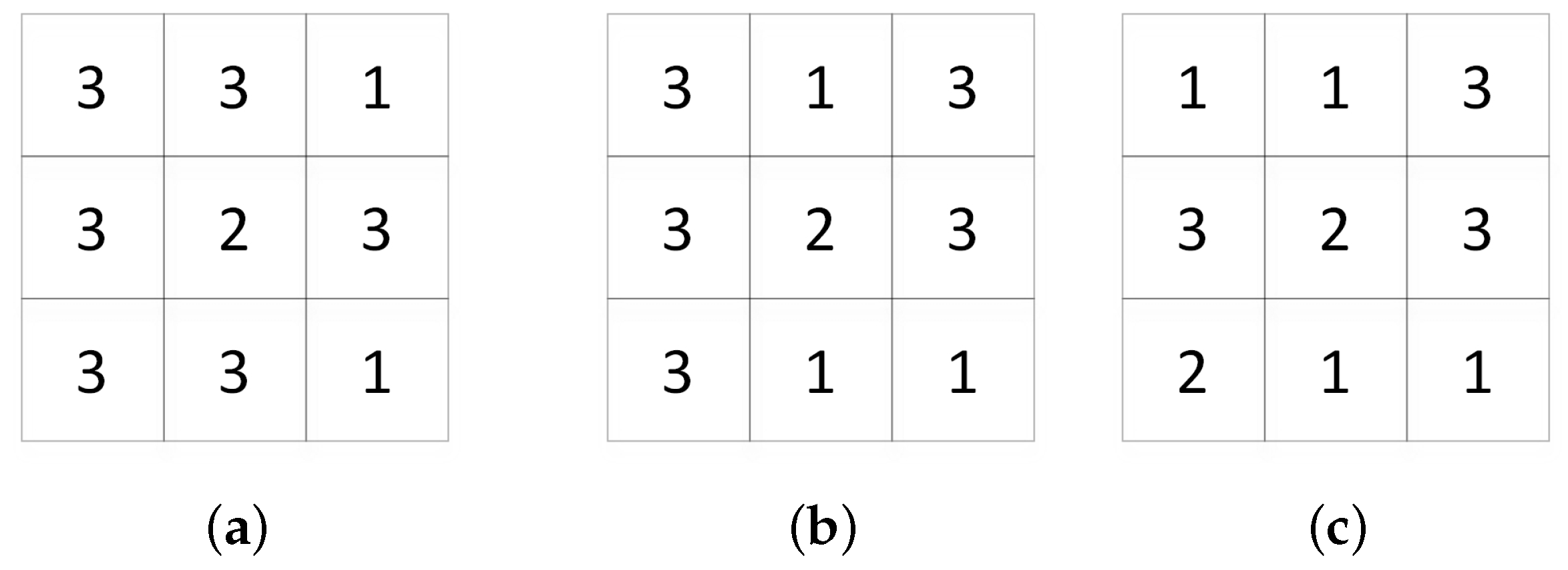
2.3. Spatial Pixel-Squares Refinement

The goal of PolSAR image classification is to assign each pixel to one class. But some pixels may be misclassified into other classes, which affects the classification accuracy. In order to reduce its impact on classification accuracy, this paper proposes a post processing method called SPF based on the blocky structure of PolSAR image. The whole algorithm is summarized in Algorithm 1. For a preliminary calssified mapping of size $w\times h$, the number of times the PixS moves in the horizontal and vertical directions is $⌊w/s⌋$ and $⌊h/s⌋$, where s is the stride of PixS movement, and ⌊⌋ indicates rounding down. $pixNu{m}_n$ represents the number of pixels of the $nth$ ($1\le n\le \left(r\times r\right)$) class in PixS.

Algorithm 1: Spatial Pixel-squares Refinement

Input: Preliminary classification result size $w\times h$, PixS size r, Stride s, Thresholds ${\tau }_0$.

while not refined all PixS do

1: Find the class with the largest number of pixels $pixNu{m}_{max}$ in PixS.

2: If $\left(r\times r\right)/2<pixNu{m}_{max}<\left(r\times r\right)$

3:    Sort all classes in PixS by the number of pixels: $pixNu{m}_{max},pixNu{m}_{2ed\_max},···$.

4:    If $\left(pixNu{m}_{max}-pixNu{m}_{2ed\_max}\right)>{\tau }_0$

5:     Refine all classes of pixels in PixS to the one class with the largest number of pixels.

6:    end if

7: end if

end while

output: refined result.

In SPF, the most critical step is to determine the refined condition. Therefore, the majority voting and difference-value methods are used as judgement rule. Specifically, majority voting is applied to find the class with the largest number of pixels $pixNu{m}_{max}$ in PixS. The size of PixS is r (r represent the number of pixels in each row or column, $r\le s$). Then compare $pixNu{m}_{max}$ with $\left(r\times r\right)/2$ to determine whether to continue processing the PixS or move to the next PixS, i.e.,

$$\left(r\times r\right)/2<pixNu{m}_{max}<\left(r\times r\right)$$

(14)

where $\left(r\times r\right)/2$ is selected to avoid that more than one category satisfies the refined condition. Here, the PixS that satisfying Equation (14) is called unstable window. In unstable window, the number of pixels belonging to each class $pixNu{m}_1,pixNu{m}_2,···,pixNu{m}_n$ need to be calculated, and sorted it then according to pixels’ number. The queue can be represented as $pixNu{m}_{max},pixNu{m}_{2ed\_max},···$. In our work, SPF refines all the classes in unstable window that satisfy the next refined condition into the one class. Therefore, to reduce computational complexity, difference–value method is employed to calculate the difference of first two classes. Then comparing the result with setting threshold ${\tau }_0$, the next refined condition can be calculated by

$$\left(pixNu{m}_{max}-pixNu{m}_{2ed\_max}\right)>{\tau }_0$$

(15)

If both Equations (14) and (15) are established, all pixels in PixS are changed to the category with the largest number of pixels.

The diagram of SPF is shown in Figure 2. Left shows unprocessed PixS, the refined result is displayed in right picture.

In SPF, the size of the PixS is one of the most crucial factors affecting the refinement results. It is proved it by experiment that the larger size of PixS incorrectly refines other class of pixels in the edge of land cover, and smaller size affects the efficiency of refinement. The optimal result can be obtained by setting the size of PixS to $3\times 3$ and the threshold ${\tau }_0$ to 3.

There are three different cases of PixS to be refined in Figure 3. Each digit in the PixS represents a pixel class.

When $r=3$, we have $\left(r\times r\right)/2=\left(3\times 3\right)/2$. Let $num\left(y_c=m\right)$ denote the number of pixels of class m, here $m\in \left\{1,2,3\right\}$. In Figure 3a, $num\left(y_c=3\right)=6>\left(3\times 3\right)/2$, $num\left(y_c=1\right)=2$, and $num\left(y_c=2\right)=1$, $pi{x}_{max}-pi{x}_{2ed\_max}=6-2=4>{\tau }_0$. Hence, the classes of all pixels in PixS are changed into 3. In Figure 3b, $num\left(y_c=3\right)=5>\left(3\times 3\right)/2$, $num\left(y_c=1\right)=3$, and $num\left(y_c=2\right)=1$. But $pi{x}_{max}-pi{x}_{2ed\_max}=5-3=2<{\tau }_0$. Therefore, this PixS should maintain unchanged. In Figure 3c, $num\left(y_c=3\right)=3<\left(3\times 3\right)/2$. Keep it also unchanged.

3. Experimental Results and Discussion

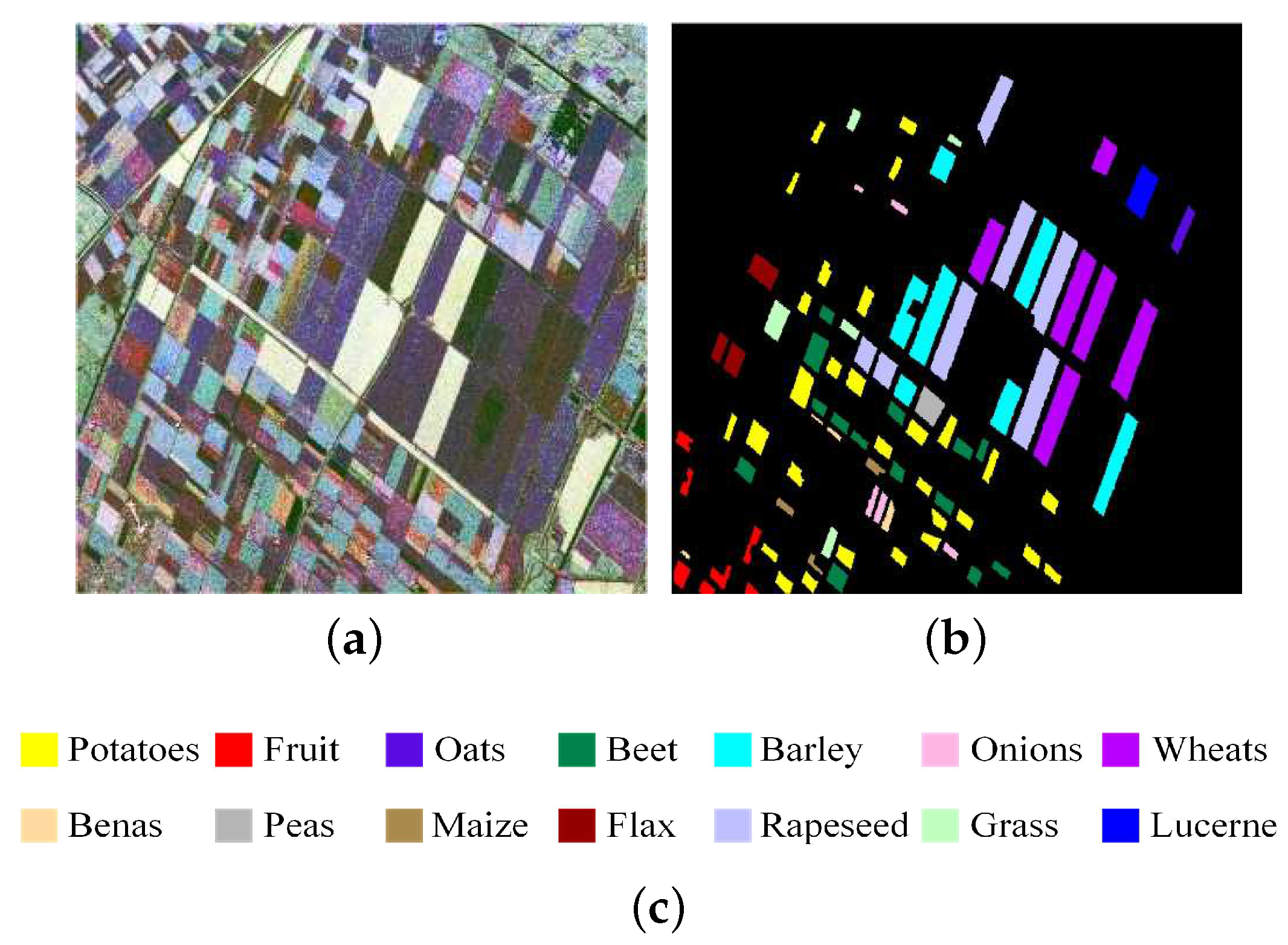
3.1. PolSAR Datasets

3.1.1. PolSAR Data Preprocessing

The scattering characteristics of pixels in PolSAR images are represented by a scattering matrix S [38]. It is defined as

$$S=\left[\begin{array}{cc}{S}_{HH}& S_{HV}\\ S_{VH}& S_{VV}\end{array}\right]$$

(16)

Generally, covariance matrix or coherent matrix are used as the unit of PolSAR image [39]. In CV-CAE, covariance matrix is adopted. Covariance matrix contains all the polarization information of object obtained by radar measurement. And it is deduced from scattering matrix. The effectiveness of covariance matrix has been authenticated in [40]. According to reciprocity theorem $S_{HV}=S_{VH}$, scattering vector is $\mathbf{x}=\left[S_{HH}\sqrt{2}{S}_{HV}{S}_{VV}\right]$. Covariance matrix can be calculated by the kronecker product of the $\mathbf{x}$ as follows

$$\mathbf{C}=\mathbf{x}{\mathbf{x}}^{\mathrm{H}}=\left[\begin{array}{ccc}〈{\left|S_{HH}\right|}^2〉& \sqrt{2}〈S_{HH}{S_{HV}}^{\ast }〉& 〈S_{HH}{S_{VV}}^{\ast }〉\\ \sqrt{2}〈S_{HV}{S_{HH}}^{\ast }〉& \sqrt{2}〈{\left|S_{HV}\right|}^2〉& \sqrt{2}〈S_{HV}{S_{VV}}^{\ast }〉\\ 〈S_{VV}{S_{HH}}^{\ast }〉& \sqrt{2}〈S_{VV}{S_{HV}}^{\ast }〉& 〈{\left|S_{VV}\right|}^2〉\end{array}\right]$$

(17)

where the superscript *, $\mathrm{T}$, $\mathrm{H}$ represent conjugation, transposition and conjugate transposition respectively. In order to suppress the speckle noise of PolSAR images, multi-look processing is introduced in covariance matrix

$$〈\mathbf{C}〉=\frac{1}{L}\sum _{i=1}^L{\mathbf{x}}_i{\mathbf{x}}_i^{\mathrm{H}}=\left[\begin{array}{ccc}{C}_{11}& C_{12}& C_{13}\\ C_{21}& C_{22}& C_{23}\\ C_{31}& C_{32}& C_{33}\end{array}\right]$$

(18)

where L is the number of looks. And ${\mathbf{x}}_i$ is the scattering vector of the $ith$ look. It can be known from the scattering properties of the PolSAR images that elements on the principal diagonal of the covariance matrix $〈\mathbf{C}〉$ are real values. The rest are complex values and conjugated at the symmetric position of the main diagonal. i.e., $C_{12}$ corresponds to $C_{21}$, $C_{13}$ corresponds to $C_{31}$, and $C_{23}$ corresponds to $C_{32}$ are conjugated. To reduce redundancy while preserving the integrity of input information, the upper triangular elements $\left\{C_{11},C_{12},C_{13},C_{22},C_{23},C_{33}\right\}$ of $〈\mathbf{C}〉$ are employed as input of the CV-CAE.

In computer vision, data normalization can effectively avoid the problem of vanishing gradient and exploding gradient, and improve the convergence efficiency of propoded network [25]. So the real values (diagonal elements) and complex values (non-diagonal elements) of input data need to be preprocessed. Taking the first channel $C_{11}$ as an example of real values

$${\tilde{C}}_{11}=\frac{C_{11}-{\mu }_{C_{11}}}{\sqrt{{\delta }_{C_{11}}^2}}$$

(19)

where ${\tilde{C}}_{11}$ is the normalized result of $C_{11}$, ${\mu }_{C_{11}}$ and ${\delta }_{C_{11}}^2$ are the average and standard deviation of $C_{11}$. They can be defined as

$${\mu }_{C_{11}}=\frac{1}{n}\sum _{i=1}^n{C}_{11}^{\left(i\right)}$$

(20)

$${\delta }_{C_{11}}^2=\frac{1}{n}\sum _{i=1}^n{\left(C_{11}^{\left(i\right)}-{\mu }_{C_{11}}\right)}^2$$

(21)

Taking the second channel $C_{12}$ as an example of complex values

$${\tilde{C}}_{12}=\frac{C_{12}-{\mu }_{C_{12}}}{\sqrt{{\delta }_{C_{12}}^2}}$$

(22)

where the average ${\mu }_{C_{12}}$ and standard deviation ${\delta }_{C_{12}}^2$ of $C_{12}$ are calculated by

$${\mu }_{C_{12}}=\frac{1}{n}\sum _{i=1}^n{C}_{12}^{\left(i\right)}$$

(23)

$${\delta }_{C_{12}}^2=\frac{1}{n}\sum _{i=1}^n\left(C_{12}^{\left(i\right)}-{\mu }_{C_{12}}\right)\overline{\left(C_{12}^{\left(i\right)}-{\mu }_{C_{12}}\right)}$$

(24)

Other real values ($C_{22}$ and $C_{33}$) and complex values ($C_{13}$ and $C_{23}$) of input data are treated in the same way.

3.1.2. PolSAR Datasets for Experiment

In this paper, three PolSAR images are used to verify the performance of the proposed algorithm. These datasets are acquired with Airborne SAR (AIRSAR) platform. Two of them show agriculture areas over Flevoland in the Netherlands. There are available online at https://earth.esa.int/web/guest/missions/esa-operational-eo-missions/envisat. And the third one is AIRSAR data over San Francisco [30]. After preprocessed, the datasets are divided into training datasets and test datasets. Training datasets are 5% and the rest are used as test datasets. The spatial resolution of the test datasets is $12\times 12$ and the number of channels is 6, which are the same as that of the training datasets. Detailed analyzing is shown in the following experiments.

3.2. Comparative Algorithms

To objectively evaluate the effectiveness of the proposed method, our algorithm is compared against three state-of-the-art algorithms. They include RV-CAE, WAE, WCAE, and fixed-feature-size CNN (FFS-CNN) [41]. To ensure the fairness of comparison, firstly, the input information content of RV-CAE should be equivalent with that of CV-CAE, so the input elements of RV-CAE are designed as $\left\{C_{11},C_{22},C_{33},real\left(C_{12}\right),imag\left(C_{12}\right),real\left(C_{13}\right),imag\left(C_{13}\right),real\left(C_{23}\right),imag\left(C_{23}\right)\right\}$. Secondly, the number of parameters in CV-CAE and RV-CAE must be the same. Therefore, in the experiment, we configure the structure and the number of parameters of RV-CAE according to

Table 2. The Structure and Parameters Number of RV-CAE and CV-CAE.

Layer NO.	RV-CAE		CV-CAE
	Architecture	Parameters	Architecture	Parameters
1	Input Layer	-	Input Layer	-
2	Conv.16 (5 × 5 × 9)/sigmoid	3600	Conv.12 (5 × 5 × 6)/sigmoid	1800 × 2
3	Mean-Po.2 (2 × 2)	-	Mean-Po.2 (2 × 2)	-
4	Upsampl (2 × 2)	-	Upsampl (2 × 2)	-
5	Deconv.9 (5 × 5 × 16)/sigmoid	3600	Deconv.6 (5 × 5 × 12)/sigmoid	1800 × 2
6	Fully Connected	$S_{Rw}\times S_{Rh}\times N$	Fully Connected	$S_{Cw}\times S_{Ch}\times N\times 2$

. In this table, “parameters” indicate the number of parameters in each layer. $S_{Rw}\times S_{Rh}$ and $S_{Cw}\times S_{Ch}$ represent the size of feature mapping of mean pooling in RV-CAE and CV-CAE respectively. N is the number of terrain type.

The structure of RV-CAE is same as that of CV-CAE. But, the input size of RV-CAE is $12\times 12$ with 9 channels. However, the number of parameters in complex domain is double of that in real domain. Therefore, in order to make sure the parameters of RV-CAE same as CV-CAE, the number of feature mappings is set 16 in RV-CAE. The quantity of parameters is $5\times 5\times 9\times 16$. Which is equal to the $5\times 5\times 6\times 12\times 2$ in CV-CAE. In CV-CAE and RV-CAE, the number of parameters of fully connected layer is the product of neurons number of input layer and output layer. In CV-CAE, the number of neurons of input layer is $S_{Cw}\times S_{Ch}$, while $S_{Rw}\times S_{Rh}$ in RV-CAE, which are feature mappings of mean pooling layer after reshaping.

3.3. Results and Analysis of Experiments

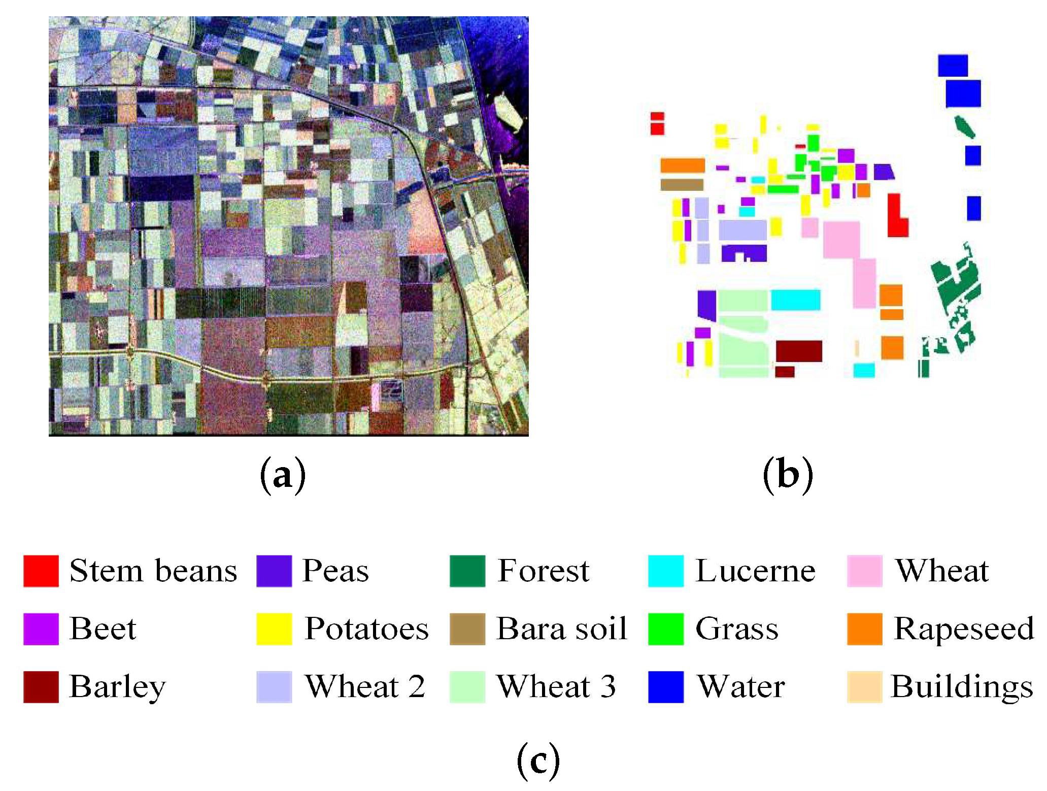
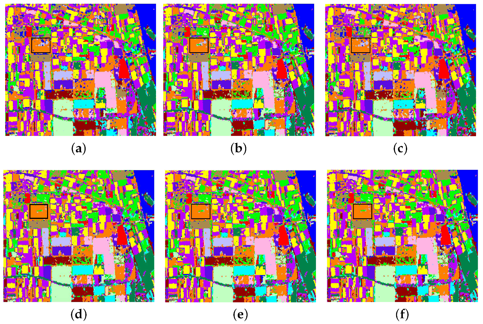
3.3.1. Experiment on Flevoland Datasets of 14 Classes

The first experiment is carried on the datasets over Flevoland, which is a subset of an L-band, full PolSAR image, attained by AIRSAR platform in 1991. It is widely applied as a benchmark data for PolSAR image classification research. The Pauli RGB image and the corresponding ground-truth are exhibited in Figure 4a,b, its size is 1020 × 1024 pixels. There are in total 14 identified classes including Potatoes, Fruit, Oats, Beet, Barley, Onions, Wheats, Beans, Peas, Maize, Flax, Rapeseed, Grass, and Lucerne. Each color indicates a type of class in ground-truth map, the corresponding legends are listed in Figure 4c.

The structure of the network is shown in Figure 1. Hyperparameters were selected as follows. Firstly, unsupervised training processe is employed to train CV-CAE with learning rate 0.001. Then the annotated training data is utilized to train CFC and fine tune encoding of CV-CAE. In supervised training processes, learning rate $\eta$ is 0.48, and the batchsize is 100. In CFC, the number of neurons of the input layer is 192, and the output layer is 14.

For convenience, the proposed methods CV-CAE add SPF are abbreviated to CV-CAE+SPF. The classification results of the compared algorithms and the proposed algorithm are shown in Figure 5. The notable different results are highlighted by black rectangle. Comparing Figure 5a,c, the number of misclassified pixels of CV-CAE are clearly less than that of the compared RV-CAE. And the intra-class of the classification map of CV-CAE is smoother than that of RV-CAE. As is shown in the lower left of Figure 5a,c, CV-CAE achieves the more distinguishable edge. In Figure 5a,b, the number of misclassified pixels is further depressed by CV-CAE+SPF. CV-CAE+SPF achieves the best classification result compared with other two algorithms.

The classified accuracy of each class, OA and Kappa are listed in

Table 3. The OA and Kappa Coefficient of Our Algorithms and the Compared Algorithms.

Class	WAE	WCAE	RV-CAE	CV-CAE	CV-CAE+SPF
Potatoes	89.83	99.78	99.69	99.79	99.8
Fruit	97.62	88.2	94.76	97.09	98.07
Oats	98.92	98.28	98.78	100	100
Beet	89.66	91.72	90.03	92.51	92.77
Barley	97.27	95.96	99.51	99.79	99.78
Onions	81.48	85.69	97.42	91.88	90.7
Wheats	89.47	94.91	99.76	99.86	99.87
Beans	87.52	91.04	82.9	92.7	95.56
Peas	89.95	91.49	99.91	99.54	99.77
Maize	94.19	99.05	95.5	98.6	98.84
Flax	94.49	89.12	94.02	95.54	96.56
Rapeseed	89.62	94.73	99.9	99.93	99.94
Grass	84.59	97.23	97.38	96.12	96.88
Luceme	96.34	97.46	99.73	98.61	98.2
OA	96.53	97.49	98.34	98.7	98.82
Kappa	0.96	0.97	0.98	0.984	0.986

, and the best results are shown in bolding. From Table 3, we can know that the CV-CAE+SPF obtained the best accuracy than the CV-CAE and RV-CAE. The OA of RV-CAE, CV-CAE and CV-CAE+SPF are 98.34%, 98.7%, and 98.82% respectively. And the Kappa coefficients also achieve improvement in our algorithms including CV-CAE and CV-CAE+SPF. This indicates the effectiveness of our methods. Specifically, the accuracy of Oats is 100%, which is achieved by the proposed methods. And the accuracy of Beans in CV-CAE is 92.7% while RV-CAE is only 82.9%. These results illustrate that phase information is a crucial feature in PolSAR image classified tasks.

In addition, the classification accuracy CV-CAE+SPF is further improved compared with CV-CAE in Table 3, which indicates the success of SPF. Furthermore, another experment is carried out to evaluate the effectiveness of proposed SPF. The result shown that the proposed SPF takes 4.39 s while improving the correct rate by 0.12%. And the compated algorithm (pixel-by-pixel refinement based on majority vote) takes 70.95 s while increasing the correct rate by only 0.04%. However, the proposed algorithm achieves a lower accuracy rate on Onions. From the confusion matrix of CV-CAE+SPF shown in

Table 4. The Confusion Matrix of CV-CAE+SPF.

%	1	2	3	4	5	6	7	8	9	10	11	12	13	14
1	99.8	0	0	0	0	0.03	0.01	0	0	0	0	0.13	0	0.02
2	0.32	98.07	0	0.26	0.21	0.03	0.03	0	1.03	0	0.05	0	0	0
3	0	0	100	0	0	0	0	0	0	0	0	0	100	0
4	0	0	0	92.77	0.01	6.83	0.03	0.04	0	0	0	0.01	0	0
5	0	0	0.02	0	99.78	0	0.19	0	0	0	0	0	0.02	0
6	0.38	0	0	1.6	0.38	90.7	1.17	1.46	0.14	1.55	0	0	0	0.05
7	0	0	0.09	0	0	0.03	99.87	0	0	0	0	0	0.09	0.01
8	0	0	0	0	0	4.25	0	95.56	0	0	0	0	0	0
9	0	0	0	0	0	0.23	0	0	99.77	0	0	0	0	0
10	0	0	0	0.23	0	0.85	0	0	0	98.84	0	0	0.08	0
11	0	0	0	0	0.05	0.42	0	1.53	0	0	96.56	0	1.44	0
12	0	0.03	0	0	0	0	0.02	0	0	0	0	99.94	0	0
13	0.64	0	0	0	0	1.05	1.43	0	0	0	0	0	96.88	0
14	0	0	0	0	0	1.42	0.37	0	0	0	0	0	0	98.2

(Each row in the table indicates the natural class, and each column indicates the predicted class. 1 to 14 represent the Potatoes, Fruit, Oats, Beet, Barley, Onions, Wheats, Beans, Peas, Maize, Flax, Rapeseed, Grass, Lucerne), we can know that Beet, Wheats, Beans, and Maize take the large ratio of misclassified classes of Onions. Considering the ground-truth in Figure 4b, it can be found that the annotated area of Onions is smaller than other classes such as Potatoes, Barely, and Wheats. Consequently, many of the input patch is smaller than $12\times 12$ in size and needed zero padding, which leads to the discriminant features cannot be extracted adequately.

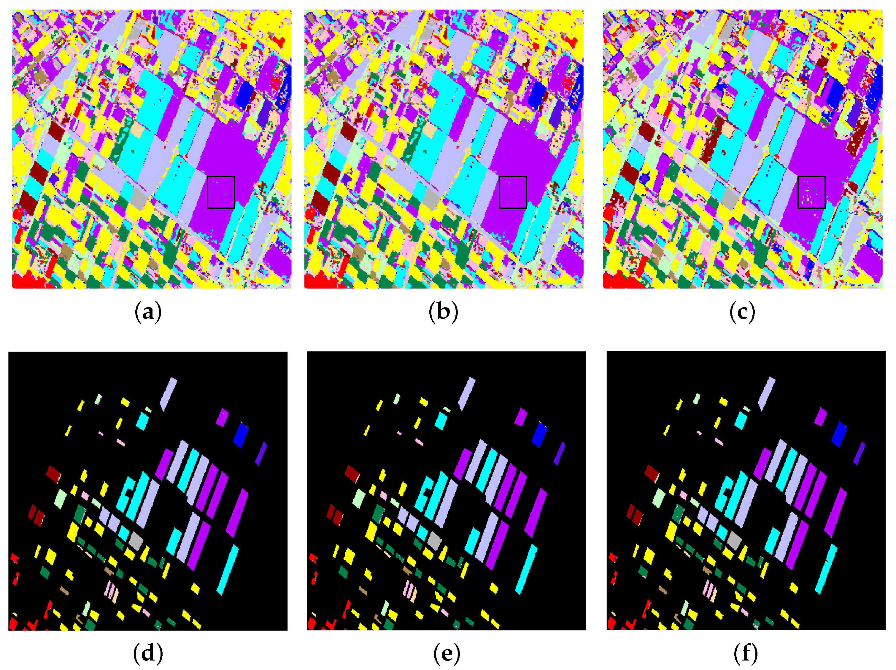
3.3.2. Experiment on Flevoland Datasets of 15 Classes

In this experiment, the datasets acquired by AIRSAR platform in 1989. Pauli RGB image and the corresponding ground-truth are shown in Figure 6a,b, whose size is 750 × 1024 pixels. According to the ground-truth, there are 15 classes including Stem beans, Peas, Forest, Lucerne, Wheat, Beet, Potatoes, Bara soil, Grass, Rapeseed, Barley, Wheat2, Wheat3, Water, and Buildings. The structure of the network and the ratio of training datasets are chosen the same as the previous experiment. Here, the hyperparameters of proposed algorithms are selected the same as those in the experiments of Flevoland of 14 classes. However, learning rate $\eta$ is 0.43, and the number of output neurons is 15.

As is shown in Figure 7, the classification results of WAE, WCAE, RV-CAE, FFS-CNN, CV-CAE and CV-CAE+SPF corresponding from a to f. It can be seen from Figure 7a,c that most pixels of Rapeseed are misclassified into Water and Wheat2. And in Figure 7b, many pixels of Rapeseed are misclassified into Grass and Wheat2. To evaluate the performance of the proposed method, the comparison is made between the compared methods and the proposed methods. It can be observed from Figure 7e,f that the number of misclassified pixels are lower than that of compared algorithms. Therefore, CV-CAE and CV-CAE+SPF give the best performance. In addition, the intra-class smoothness and the inter-class distinctness of the proposed algorithms are better than that of the compared algorithms.

The classification accuracy of the proposed algorithms and the compared algorithms is listed in

Table 5. The OA and Kappa Coefficient of Our Algorithms and the Compared Algorithms.

Class	WAE	WCAE	RV-CAE	FFS-CNN	CV-CAE	CV-CAE+SPF
Stem beans	88.02	93.09	88.2	93	92.25	93.56
Peas	91.49	92.36	87.95	93.21	92.26	93.52
Forest	97.89	98.74	97.12	98.97	98.74	99.21
Lucerne	88.5	89.22	90.69	91.98	91.18	92.24
Wheat	91.48	94.51	94.72	95.41	94.89	95.38
Beet	84.7	91.01	80.25	91.85	90.9	93.09
Potatoes	81.94	87.21	77.56	88.63	86.93	89.24
Bare soil	97.92	99.42	100	99.09	99.12	99.35
Grass	69.82	82.17	73.14	85.91	84.42	87.02
Rapeseed	92.66	91.03	91.91	93.54	92.96	93.24
Barley	96.89	93.83	94.34	94.34	93.45	94.88
Wheat2	87.84	90.91	88.98	91.09	90.42	91.65
Wheat3	94.85	96.6	95.29	97.08	96.76	97.13
Water	98.67	96.66	99.05	97.76	97.56	97.72
Buildings	86.55	87.09	82.14	90.55	90.55	90.13
OA	90.74	92.94	90.39	94	93.31	94.31
Kappa	0.9	0.92	0.89	0.935	0.93	0.94

. CV-CAE and CV-CAE+SPF achieve better OA than the compared algorithms, followed by WCAE, WAE, and RV-CAE. In this experiment, WAE performs not well in recognizing Beet, Potatoes, and Grass. The accuracy of these classes is lower than 85% while CV-CAE+SPF achieved 93.09%, 89.24% and 87.02% respectively. Moreover. RV-CAE cannot distinguish Potatoes, Grass and Buildings clearly, and discriminate Potatoes and Grass with the accuracy of 77.56% and 73.14%. But the proposed CV-CAE improves the accuracy of these two classes by 10 points compared with RV-CAE, and also achieves 100% accuracy on Bare soil. Therefore, phase information can promote the improvement of classification accuracy. In order to explicate the effect of SPF, a comparison of CV-CAE and CV-CAE+SPF is carried out, and the OA is increased by 1 point in CV-CAE+SPF, i.e., 94.31% is comparable to 93.31%. However, the result of FFS-CNN is higher than that of the CV-CAE, but lower than that of CV-CAE+SPF. Furthermore, FFS-CNN is based on the LeNet-5, which contains three convolutional layers with the size of convolutional kernel $3\times 3$ and feature mappings of 100. So the parameters of FFS-CNN are much larger than those of the algorithm proposed in this paper.

To evaluate the generalization of proposed SFP, which is also used to process the preliminary classification results of the compared method. The OA is improved by 0.78%, 1.03%, 1.29%, and 0.86%, of WAE, WCAE, RV-CAE, and FFS-CNN respectively.

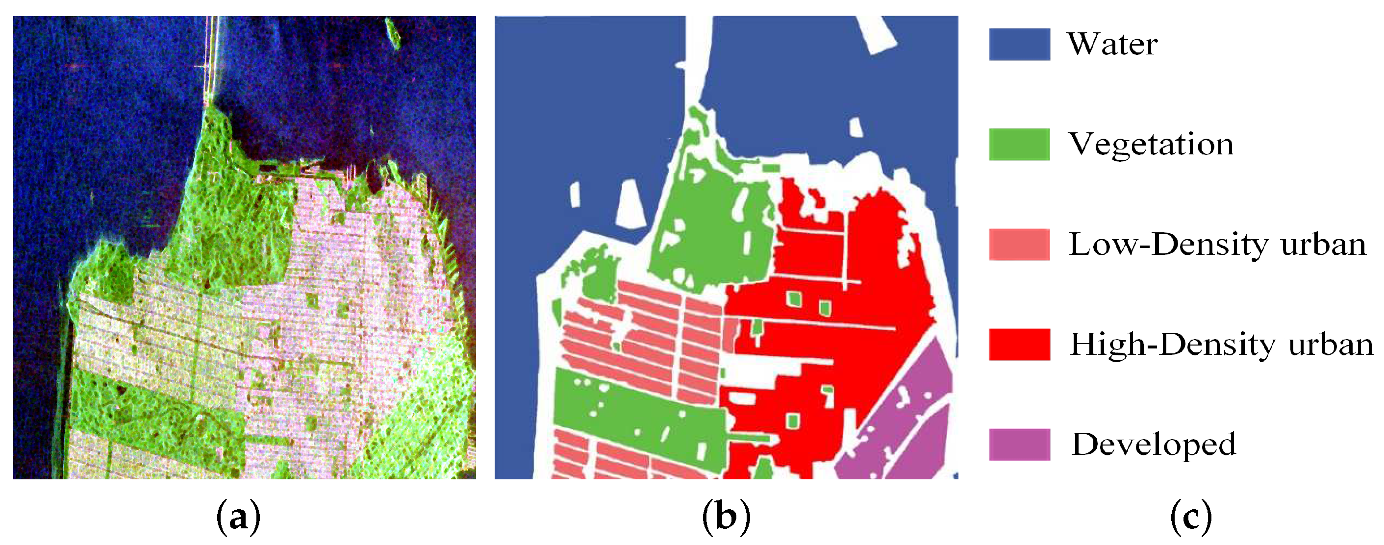
3.3.3. Experiment on San Francisco Datasets of 5 Classes

San Francisco Datasets, acquired by the AIRSAR platform, is adopted in this experiment. The Pauli RGB image and corresponding ground-truth are shown in Figure 8a,b. Five colors in ground-truth map represents five terrain types, which are vegetation, low-density urban, high-density urban, and developed. The legends are listed in Figure 8c. From Figure 8b, we can know that most of the annotated areas are irregular. Thus, the complexity of this experiment is higher than the previous two experiments.

In this experiment, learning rate $\eta$ is 0.6, the number of output neurons is 5, network structure and other hyperparameters are same as that of the above two experiments.

Table 6. The OA and Kappa Coefficient of Our Algorithms and the Compared Algorithms.

Class	WAE	WCAE	RV-CAE	CV-CAE	CV-CAE+SPF
Water	99.91	98.24	95.51	99.46	99.5
Vegetation	58.85	91.34	87.87	93.71	93.77
Low-Density urban	78.12	96.88	90.56	97.58	97.65
High-Density urban	81.43	91.29	80.76	93.06	93.26
Developed	94.08	93.63	94.15	95.54	95.88
OA	87.87	95.44	90.84	96.94	97.03
Kappa	0.81	0.93	0.86	0.95	0.96

indicates the classification results of each algorithm. For WAE, the classification accuracy of Vegetation and Low-Density urban is 58.85% and 78.12%, while CV-CAE achieves significant improvement in classification accuracy. RV-CAE cannot distinguish High-Density urban clearly with the accuracy is 80.76%. The performance of WCAE is better than that of WAE and RV-CAE in Vegetation, Low-Density urban and High-Density urban. However, the accuracy of Developed category is slightly lower than that of the above two algorithms. According to the results summarized in Table 6, compared with WCAE, 1.5 points is increased of OA by CV-CAE+SPF. However, the recognition rate of CV-CAE+SPF on Vegetation and High-Density urban is lower than that of other classes. From the confusion matrix of CV-CAE+SPF shown in

Table 7. The Confusion Matrix of CV-CAE+SPF.

%	1	2	3	4	5
1	99.5	0.44	0.01	0.04	0
2	0.39	93.77	2.77	1.47	1.59
3	0	0.36	97.65	1.99	0
4	0	0.1	6.04	93.26	0.45
5	0	3.28	0.28	0.56	95.88

(Each row in the table indicates the natural class, and each column indicates the predicted class. 1 to 5 represent Water, Vegetation, Low-Density urban, High-Density urban, Developed), we can know that there is a large proportion of these two classes of misclassification into the Low-Density urban. Therefore, the features of these two classes are similar to the Low-Density urban. It also can be verified in Figure 8b. However, associating with the phase information and SPF, CV-CAE+SPF gives the best performance. Its OA and Kappa coefficient are 97.03% and 0.96.

4. Conclusions

CAE has demonstrated significant success in computer vision. In order to take advantage of phase information of PolSAR images, the RV-CAE is extended to complex domain and CV-CAE is proposed. CV-CAE is designed to extract more discriminant features from amplitude and phase information of tiny number of unannotated training data. To fit the classification task, a small number of annotated training datasets are needed to adjust the classification network, the convolution operation of which is initialized by the trained CV-CAE. We have tested the performance of proposed CV-CAE on three PolSAR datasets and compared against several other similar models including WAE, WCAE, and RV-CAE. CV-CAE achieves the better performance than the compared algorithms. In addition, a post processing method named SPF is proposed to further improve the performance. Benefitting from the blocky structure of land cover of PolSAR images, the proposed SPF refines the class of pixels in the spatial squares at the same time, which alleviates the time-consuming problem of pixel level refinement. Compared with CV-CAE, CV-CAE+SPF further improves the classification accuracy. Future work will investigate ways of replacing a two-stage network with an end-to-end network to reduce the complexity and improve the efficiency of this network. We can also investigate the advantages of shorter time-consuming and more efficient post processing methods to achieve better results.

References

1. Van, J.J.; Burnette, C.F. Bayesian classification of polarimetric SAR images using adaptive a priori probabilities. Int. J. Remote Sens. 1992, 13, 835–840. [Google Scholar]
2. Shang, R.; Yuan, Y.; Jiao, L.; Hou, B.; Esfahani, A.M.; Stolkin, R. A Fast Algorithm for SAR Image Segmentation Based on Key Pixels. IEEE J. Sel. Top. Appl. Earth Obs. Remote Sens. 2017, 10, 5657–5673. [Google Scholar] [CrossRef]
3. Wang, Y.; He, C.; Liu, X.; Liao, M. PolSAR Land Cover Classification Based on Roll-Invariant and Selected Hidden Polarimetric Features in the Rotation Domain. Remote Sens. 2017, 9, 660. [Google Scholar] [CrossRef]
4. Szegedy, C.; Ioffe, S.; Vanhoucke, V.; Alemi, A.A. Inception-v4, inception-resnet and the impact of residual connections on learning. In Proceedings of the Thirty-First AAAI Conference on Artificial Intelligence (AAAI-17), San Francisco, CA, USA, 4–9 February 2017; p. 12. [Google Scholar]
5. Yamaguchi, Y.; Moriyama, T.; Ishido, M.; Yamada, H. Four-component scattering model for polarimetric SAR image decomposition. IEEE Trans. Geosci. Remote Sens. 2005, 43, 1699–1706. [Google Scholar] [CrossRef]
6. Zhang, Z.; Wang, H.; Xu, F.; Jin, Y. Complex-valued convolutional neural network and its application in polarimetric SAR image classification. IEEE Trans. Geosci. Remote Sens. 2017, 55, 7177–7188. [Google Scholar] [CrossRef]
7. Akbarizadeh, G. A New Statistical-Based Kurtosis Wavelet Energy Feature for Texture Recognition of SAR Images. IEEE Trans. Geosci. Remote Sens. 2012, 50, 4358–4368. [Google Scholar] [CrossRef]
8. Ghosh, A.; Subudhi, B.N.; Bruzzone, L. Integration of Gibbs Markov Random Field and Hopfield-Type Neural Networks for Unsupervised Change Detection in Remotely Sensed Multitemporal Images. IEEE Trans. Image Process. 2013, 22, 3087–3096. [Google Scholar] [CrossRef] [PubMed]
9. Bombrun, L.; Beaulieu, J.M. Fisher Distribution for Texture Modeling of Polarimetric SAR Data. IEEE Geosci. Remote Sens. Lett. 2008, 5, 512–516. [Google Scholar] [CrossRef] [Green Version]
10. Lee, T.S. Image Representation Using 2D Gabor Wavelets. IEEE Geosci. Remote Sens. Lett. 1996, 18, 959–971. [Google Scholar]
11. Hu, J.; He, Z.; Li, J.; He, L.; Wang, Y. 3D-Gabor Inspired Multiview Active Learning for Spectral-Spatial Hyperspectral Image Classification. Remote Sens. 2018, 10, 1070. [Google Scholar] [CrossRef]
12. Freeman, A.; Villasenor, J.; Klein, J.D.; Hoogeboom, P.; Groot, J. On the use of multi-frequency and polarimetric radar backscatter features for classification of agricultural crops. Int. J. Remote Sens. 1994, 15, 1799–1812. [Google Scholar] [CrossRef]
13. Du, L.; Lee, J.; Hoppel, K.; Mango, S.A. Segmentation of SAR images using the wavelet transform. Int. J. Imaging Syst. Technol. 1992, 4, 319–326. [Google Scholar] [CrossRef]
14. Lee, J.S.; Grunes, M.R.; Ainsworth, T.L.; Du, L.J.; Schuler, D.L.; Cloude, S.R. Unsupervised classification using polarimetric decomposition and the complex Wishart classifier. IEEE Trans. Geosci. Remote Sens. 1999, 37, 2249–2258. [Google Scholar]
15. Hou, B.; Kou, H.; Jiao, L. Classification of polarimetric SAR images using multilayer autoencoders and superpixels. IEEE J. Sel. Top. Appl. Earth Obs. Remote Sens. 2016, 9, 3072–3081. [Google Scholar] [CrossRef]
16. Zhao, Q.; Principe, J.C. Support vector machines for SAR automatic target recognition. IEEE Trans. Aerosp. Electron. Syst. 2001, 37, 643–654. [Google Scholar] [CrossRef]
17. Loosvelt, L.; Peters, J.; Skriver, H.; Baets, B.; Verhoest, N. Impact of reducing polarimetric SAR input on the uncertainty of crop classifications based on the random forests algorithm. IEEE Trans. Geosci. Remote Sens. 2012, 50, 4185–4200. [Google Scholar] [CrossRef]
18. Uhlmann, S.; Kiranyaz, S. Integrating color features in polarimetric SAR image classification. IEEE Trans. Geosci. Remote Sens. 2014, 52, 2197–2216. [Google Scholar] [CrossRef]
19. LeCun, Y.; Bengio, Y.; Hinton, G. Deep learning. Nature 2015, 521, 436–444. [Google Scholar] [CrossRef] [PubMed]
20. Zhang, L.; Ma, W.; Zhang, D. Stacked Sparse Autoencoder in PolSAR Data Classification Using Local Spatial Information. IEEE Geosci. Remote Sens. Lett. 2016, 13, 1359–1363. [Google Scholar] [CrossRef]
21. Geng, J.; Wang, H.; Fan, J.; Ma, X. SAR Image Classification via Deep Recurrent Encoding Neural Networks. IEEE Trans. Geosci. Remote Sens. 2018, 56, 2255–2269. [Google Scholar] [CrossRef]
22. De, S.; Bruzzone, L.; Bhattacharya, A.; Bovolo, F.; Chaudhuri, S. A Novel Technique Based on Deep Learning and a Synthetic Target Database for Classification of Urban Areas in PolSAR Data. IEEE J. Sel. Top. Appl. Earth Obs. Remote Sens. 2018, 11, 154–170. [Google Scholar] [CrossRef]
23. Shang, R.; Wang, J.; Jiao, L.; Stolkin, R.; Hou, B.; Li, Y. SAR Targets Classification Based on Deep Memory Convolution Neural Networks and Transfer Parameters. IEEE J. Sel. Top. Appl. Earth Obs. Remote Sens. 2018, 11, 2834–2846. [Google Scholar] [CrossRef]
24. Gao, Q.; Lim, S.; Jia, X. Hyperspectral Image Classification Using Convolutional Neural Networks and Multiple Feature Learning. Remote Sens. 2018, 10, 299. [Google Scholar] [CrossRef]
25. Hosseini, A.E.; Zurada, J.M.; Nasraoui, O. Deep learning of part-based representation of data using sparse autoencoders with nonnegativity constraints. IEEE Trans. Neural Netw. Learn. Syst. 2016, 27, 2486–2498. [Google Scholar] [CrossRef] [PubMed]
26. Masci, J.; Meier, U.; Ciresan, D.; Schmidhuber, J. Stacked convolutional auto-encoders for hierarchical feature extraction. In Proceedings of the 21st International Conference on Artificial Neural Networks, Espoo, Finland, 14–17 June 2011; pp. 52–59. [Google Scholar]
27. Deng, S.; Du, L.; Li, C.; Ding, J.; Liu, H. SAR automatic target recognition based on euclidean distance restricted autoencoder. IEEE J. Sel. Top. Appl. Earth Obs. Remote Sens. 2017, 10, 3323–3333. [Google Scholar] [CrossRef]
28. Chen, M.; Wang, Q.; Li, X. Discriminant Analysis with Graph Learning for Hyperspectral Image Classification. Remote Sens. 2018, 10, 836. [Google Scholar] [CrossRef]
29. Chen, W.; Gou, S.; Wang, X.; Li, X.; Jiao, L. Classification of PolSAR Images Using Multilayer Autoencoders and a Self-Paced Learning Approach. Remote Sens. 2018, 10, 110. [Google Scholar] [CrossRef]
30. Xie, W.; Jiao, L.; Hou, B.; Ma, W.; Zhao, J.; Zhang, S.; Liu, F. POLSAR image classification via Wishart-AE model or Wishart-CAE model. IEEE J. Sel. Top. Appl. Earth Obs. Remote Sens. 2017, 10, 3604–3615. [Google Scholar] [CrossRef]
31. Liu, F.; Jiao, L.; Hou, B.; Yang, S. POL-SAR Image Classification Based on Wishart DBN and Local Spatial Information. IEEE Trans. Geosci. Remote Sens. 2016, 54, 3292–3308. [Google Scholar] [CrossRef]
32. Liu, H.; Yang, S.; Gou, S.; Chen, P.; Wang, Y.; Jiao, L. Fast Classification for Large Polarimetric SAR Data Based on Refined Spatial-Anchor Graph. IEEE Trans. Geosci. Remote Sens. 2017, 14, 1589–1593. [Google Scholar] [CrossRef]
33. Ulaby, F.T.; Charles, E. Radar Polarimetry for Geoscience Applications; Artech House, Inc.: Norwood, MA, USA, 1990; 376p. [Google Scholar]
34. Marques, P.A.; Dias, J.M. Moving Targets Processing in SAR Spatial Domain. IEEE Trans. Geosci. Remote Sens. 2007, 43, 864–874. [Google Scholar] [CrossRef]
35. Boureau, Y.L.; Bach, F.; LeCun, Y.; Ponce, J. Learning mid-level features for recognition. In Proceedings of the Twenty-Third IEEE Conference on Computer Vision and Pattern Recognition, San Francisco, CA, USA, 13–18 June 2018; pp. 2559–2566. [Google Scholar]
36. Karen, S.; Andrew, Z. Very deep convolutional networks for large-scale image recognition. arXiv, 2009; arXiv:1409.1556. [Google Scholar]
37. Xavier, G.; Bordes, A.; Bengio, Y. Deep sparse rectifier neural networks. In Proceedings of the Fourteenth International Conference on Artificial Intelligence and Statistics, Fort Lauderdale, FL, USA, 11–14 April 2011; pp. 315–323. [Google Scholar]
38. Li, Y.; Chen, Y.; Liu, G.; Jiao, L. A Novel Deep Fully Convolutional Network for PolSAR Image Classification. Remote Sens. 2018, 10, 1984. [Google Scholar] [CrossRef]
39. Biondi, F. Multi-chromatic analysis polarimetric interferometric synthetic aperture radar (MCAPolInSAR) for urban classification. Int. J. Remote Sens. 2018, 1–30. [Google Scholar] [CrossRef]
40. Chen, S.; Wang, X.; SatoLi, M. PolInSAR Complex Coherence Estimation Based on Covariance Matrix Similarity Test. IEEE Trans. Geosci. Remote Sens. 2012, 50, 4699–4710. [Google Scholar] [CrossRef]
41. Wang, L.; Xu, X.; Dong, H.; Gui, R.; Pu, F. Multi-Pixel Simultaneous Classification of PolSAR Image Using Convolutional Neural Networks. Sensors 2018, 18, 769. [Google Scholar] [CrossRef] [PubMed]
Figure 1. CV-CAE architecture. Red and blue boxes are the structure of the CV-CAE and classification network respectively.
Remotesensing 11 00522 g001
Figure 2. The refinement process of SPF. the shaded part represents p i x N u m max , the blank part represents other classes.
Remotesensing 11 00522 g002
Figure 3. PixS to be refined in three different cases.
Remotesensing 11 00522 g003
Figure 4. Flevoland datasets of 14 classes. (a) Pauli RGB. (b) Ground-truth map. (c) Legends.
Remotesensing 11 00522 g004
Figure 5. The classification results and the result overlaid with ground-truth of our algorithm and RV-CAE. (a,d) are result of CV-CAE. (b,e) are result of CV-CAE+SPF. (c,f) are result of RV-CAE.
Remotesensing 11 00522 g005
Figure 6. Flevoland datasets of 15 classes. (a) Pauli RGB. (b) Ground-truth map. (c) Legends.
Remotesensing 11 00522 g006
Figure 7. The classification results of our algorithms and compared algorithms. (a) WAE. (b) WCAE. (c) RV-CAE. (d) FFS-CNN. (e) CV-CAE. (f) CV-CAE+SPF.
Remotesensing 11 00522 g007
Figure 8. San Francisco datasets of 5 class. (a) Pauli RGB. (b) Corresponding Ground-truth. (c) Legends.
Remotesensing 11 00522 g008