Mapping Pure Mangrove Patches in Small Corridors and Sandbanks Using Airborne Hyperspectral Imagery


1
Global Earth Observation and Data Analysis Centre, National Cheng Kung University, Tainan 70101, Taiwan
2
Department of Earth Sciences, National Cheng Kung University, No 1, Ta-Hsueh Road, Tainan 70101, Taiwan
3
Endemic Species Research Institute, Council of Agriculture, Chi-Chi, Nantou 55244, Taiwan
*
Author to whom correspondence should be addressed.
Remote Sens. 2019, 11(5), 592; https://0-doi-org.brum.beds.ac.uk/10.3390/rs11050592
Submission received: 25 January 2019
/
Revised: 5 March 2019
/
Accepted: 7 March 2019
/
Published: 12 March 2019
(This article belongs to the Special Issue Remote Sensing of Mangroves)
Abstract
:Taijiang National Park (TNP) of Taiwan is the northernmost geographical position of mangrove habitats in the Northern Hemisphere. Instead of occupying a vast region with a single species, the mangroves in TNP are usually mingled with other plants in a narrow corridor along the water or in groups on a small sandbank. The multi-spectral images acquired from the spaceborne platforms are therefore limited in mapping the abundance and distribution of the mangrove species in TNP. We report the work of mapping pure mangrove patches in small corridors and sandbanks in TNP using airborne Compact Airborne Spectrographic Imager (CASI) hyperspectral imagery. Bu considering the similarity of spectral reflectance among three species of mangrove and other plants, we followed the concept of supervised classification to select a few training areas with known mangrove trees, where the training areas are determined from the detailed map of mangrove distribution derived from the field investigation. The Hourglass hyperspectral analysis technique was employed to identify the endmembers of pure mangrove in the training areas. The results are consistent with the current distribution of mangrove trees, and the remarkable feature of a “mangrove desert” highlights a fact that biodiversity can be easily and quickly destroyed if no protection is provided. Some remnant patches located by this research are very important to the management of mangrove trees.
1. Introduction
Thriving in a transition zone between land and sea in intertidal coastal regions, mangroves act as a pioneer of coastal ecology and an indicator of climate change. With the features of adaptations for mechanical fixation in loose soil, breathing roots and air exchange devices, specialized dispersal mechanisms, and specialized mechanisms for dealing with excess salt concentrations [1], mangroves are capable of converting a harsh and adverse salty desert into a lush and vibrant green environment. Since mangroves represent a significant sink in carbon, their response to climate change may result in either negative or positive feedback [2]. Although mangroves protect shoreline and inland areas from natural hazards (hurricanes, typhoons, tsunamis) and coastal-erosion processes [3], they cannot save themselves from the anthropogenic threats, such as the emergence of urban development, the boom in commercial aquaculture and mining, and the various forms of non-renewable exploitation [4]. It is estimated that about 36% of the total global mangrove habitat area was lost during the last two decades [5]. In the case of Taiwan, in the northernmost geographical position of mangrove habitats in the Northern Hemisphere [6], at least two species of mangroves (Ceriops tagal and bruguiera gymnorrhiza) became extinct half a century ago. Polidoro et al. [7] collected species-specific data to determine the probability of extinction for all 70 known species of mangroves. They concluded that several species at high risk of extinction may disappear well before the next decade if existing protective measures are not enforced. Retrieving up-to-date information of the extent and condition of mangrove ecosystems, therefore, is an essential aid to management and policy- and decision-making processes [3].
Compared to conventional labor-intensive and time-consuming field investigations, remote sensing offers a large-scale, long-term and cost-effective tool that is capable of providing spatiotemporal information on the mangrove ecosystem distribution, species differentiation, health status, and ongoing changes in mangrove populations [3,6]. A variety of sensors and image processing methods have long been employed in related studies [8,9], ranging from aerial photography to high- and medium-resolution optical imagery [6,10,11,12,13] and from hyperspectral data [4,14,15,16] to synthetic aperture radars (SAR) [14,17]. A comprehensive overview and sound summary of all of the work undertaken was provided by Kuenzer et al. [3]. For mapping mangroves on the species level, they concluded that hyperspectral imagery acquired from either airborne or spaceborne platforms is very promising. With close-range hyperspectral data collected either in the laboratory or in the field, not only the species level [18,19,20], but the health state and the nitrogen concentrations [21,22] can also be retrieved. As also pointed out by Kuenzer et al. [3], however, the investigations concentrate on little more than half a dozen countries. Hyperspectral mangrove-mapping research, therefore, is still in its initial stages and the final goal is to develop a standardized methodology for mangrove-mapping applications [3]. Another challenge of using remote sensing to map mangroves to a species level was presented by Heenkenda et al. [12]. Since spectral reflectance of wetland vegetation is often mixed with that of underlying wet soil and water, remote sensing data and methods that have been successfully used for classifying terrestrial vegetation communities cannot be applied to mangrove studies with the same success. They suggested that the selection of data sources for mangrove mapping should include the consideration of the ideal spectral and spatial resolutions for the species.
As the significance and threats of mangroves are recognized, more and more habitats of mangroves have been designated as conserved areas, to which access is usually highly restricted. This raises another challenge related to mapping mangroves from remote sensing: collecting end members and ground truths of surface reflectance for classification and validation. Most of the advanced techniques of hyperspectral image classification, such as the maximum likelihood classification (MLC) [6,10,14], the spectral angle mapper (SAM) [4,15,19], the neural network classification (NNC) [14], the decision tree classification (DTC) [14], and the Support Vector Machine (SVM) [12,15], all require good ground training information. Even with hundreds of spectral bands provided by hyperspectral imagery, the spectral responses among various species of mangroves are intrinsically rather similar [19]. It is, therefore, very critical to select the most useful wavebands from hyperspectral data for accurate species/condition separation [20]. Considering that the spectral reflectance of wetland vegetation is often mixed with that of underlying wet soil and water [12], a formal way of collecting ground truths is to place a field spectroradiometer on a truck-mounted boom that can be used to acquire overhead views to simulate the viewing perspective of airborne or satellite sensors [23]. However, this is not possible or it may even be forbidden to operate such a heavy truck in a conserved wetland, such as is the case in our study area: Taijiang National Park (TNP). Another challenge is that the mangroves in TNP are usually mingled with other plants in a narrow corridor along the water or in groups on a small sandbank. The multi-spectral images acquired from the spaceborne platforms with a few spectral bands and low spatial resolutions are therefore limited in mapping the abundance and distribution of mangrove species in TNP.
2. Materials and Methods
2.1. Study Site and Image Acquisition
2.1.1. Taijiang National Park
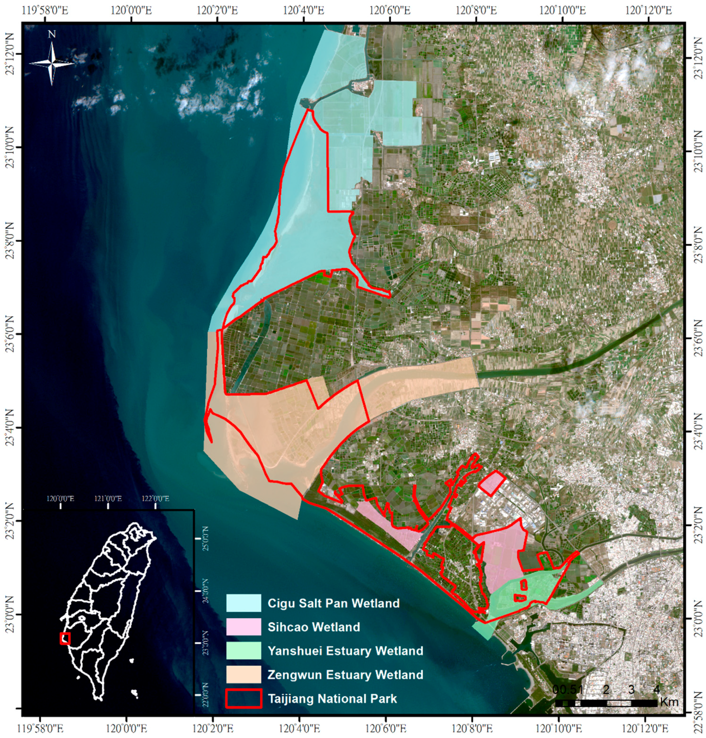
Located in the southwest coast of Taiwan, TNP is a national park in Taiwan with a total area of 39,310 hectares. Over the last few centuries, a large quantity of sand was carried by several westward-flowing rivers and deposited around the river mouths in the park. Wind, tide and waves caused the river mouths to gradually silt up and expand outwards to form four main wetland areas: Zengwen Estuary Wetland, Sicao Wetland, Qigu Salt Pan Wetland and Yanshui Estuary Wetland, as labeled in Figure 1. These wetlands enjoy abundant wildlife resources and diverse flora, including one endangered migratory bird (the black-faced spoonbill) [24] and three rare types of mangrove (Avicennia marina, Lumnitzera racemosa and Rhizophora stylosa). All of them have international ecological importance and should be protected.
A large portion of TNP was originally part of the Taijiang Inland Sea and, as a result, was inundated with brackish water. This area was gradually settled in the last few centuries and, inevitably, human activities resulted in negative impacts on the natural habitats, particularly in the case of mangrove forests. TNP was established as the eighth national park of Taiwan in 2009. One of its main missions is to protect a precious system of flora—mangroves. The first and probably the most fundamental step is to accurately and systematically map the mangroves within TNP on a regular basis. Such information will serve as a crucial source of data to understand the long-term variation in mangrove populations.
2.1.2. CASI Image Acquisition
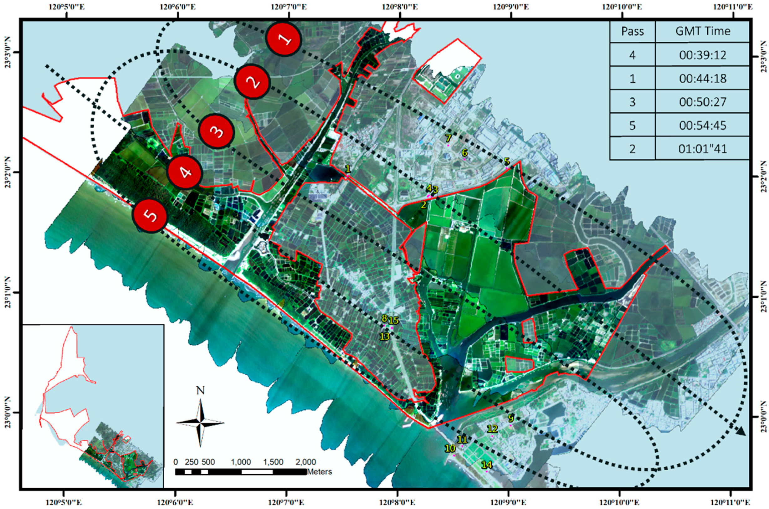
To achieve the requirement of both high-spatial- and high-spectral-resolution, hyperspectral imagery acquired from airborne instruments is preferable to that from existing spaceborne instruments (Hyperion). Zhang et al. [20] provided a full list of airborne hyperspectral instruments, such as the Airborne Visible/Infrared Imaging Spectrometer (AVIRIS), Compact Airborne Spectrographic Imager (CASI), and the Airborne Imaging Spectrometer for Application (AISA+), which have been used for monitoring and classifying mangrove species. With an extended range from 0.4 to 2.5 micron, hyperspectral instruments such as AVIRIS certainly can help in improving both the classification and the assessment of the mangrove stress status. Held et al. [14] recommended CASI because of its ease of use, high resolution, programmability of spectral band position and width, and its capability for measurement of incident light conditions. A total of 72 spectral bands ranging from 380 to 1050 nm with a narrow bandwidth (1.5 ~ 6 nm) were taken by ITRES CASI 1500 at an altitude of 1000 m on 9 September 2013, producing five strips of hyperspectral images with a spatial resolution of 1 m that covered 25 km2 of the study area, as shown in Figure 2. The entire mission was accomplished in about 23 min (from 8:39 am to 9:02 am, local time)
2.2. Surface Reflectance and Atmospheric Correction
2.2.1. Spectra of Surface Reflectance
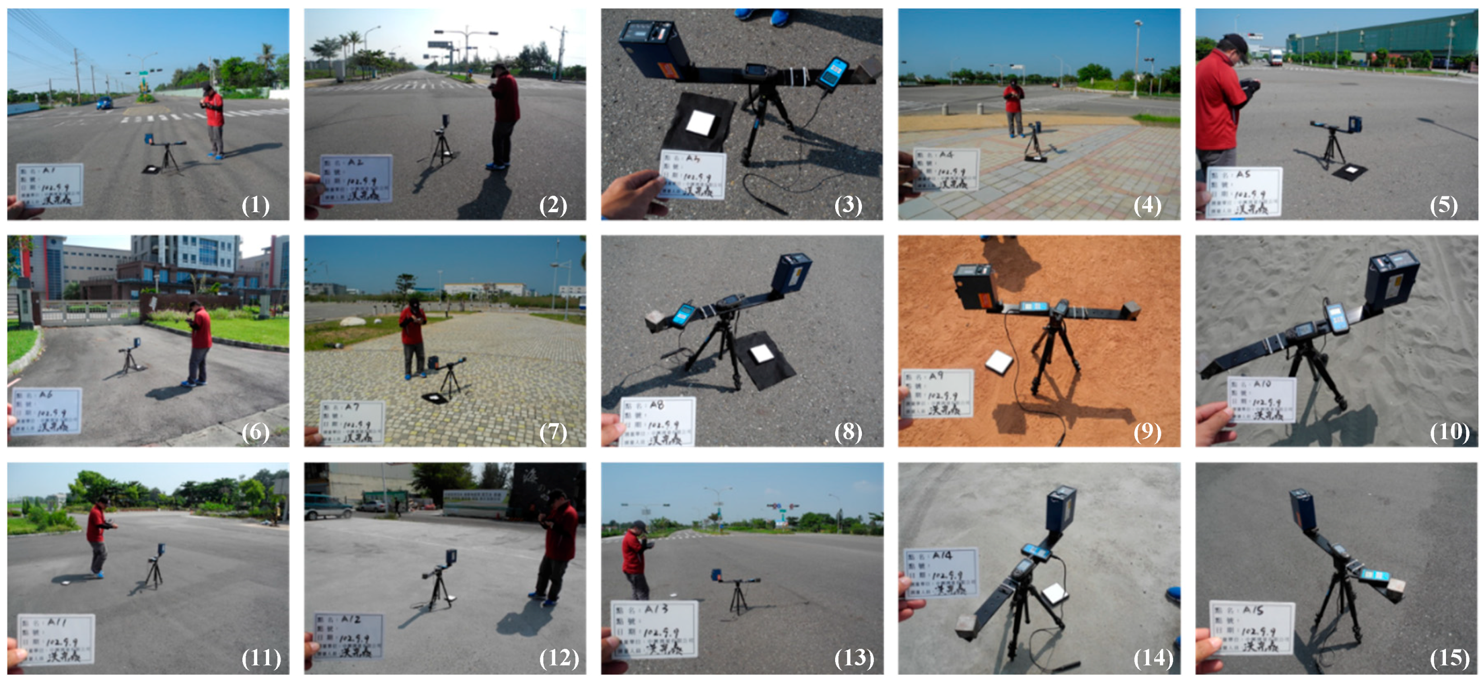
Since operating a heavy truck with a field spectroradiometer mounted on a boom to simulate the viewing perspective of CASI is forbidden inside TNP, a total of 15 sites were selected outside of TNP to collect ground truths of surface reflectance since they are covered by a large uniform area of artificial pavement, as shown in Figure 3. For these cases of large uniform surfaces, the reflectance measured on the ground is considered valid for comparing with the CASI data. As a result, most of the selected sites are covered with asphalt that is the common artificial pavement in Taiwan. Note that the collected surface reflectance is mainly used to evaluate the atmospheric correction rather than to serve as the endmembers. It is fine that no site of pure mangrove is selected to collect surface reflectance. Following the definition proposed by Heenkenda et al. [12], each site has to have a homogenous area of at least 16 m2, which is at least 16 pixels in the CASI image. The coordinates of each site were recorded using a handheld global positioning system (GPS). To overcome GPS inaccuracies, the distance of each site to water features, roads or edges of mudflats were recorded. In addition, at least 10 GPS readings were averaged for the final location.
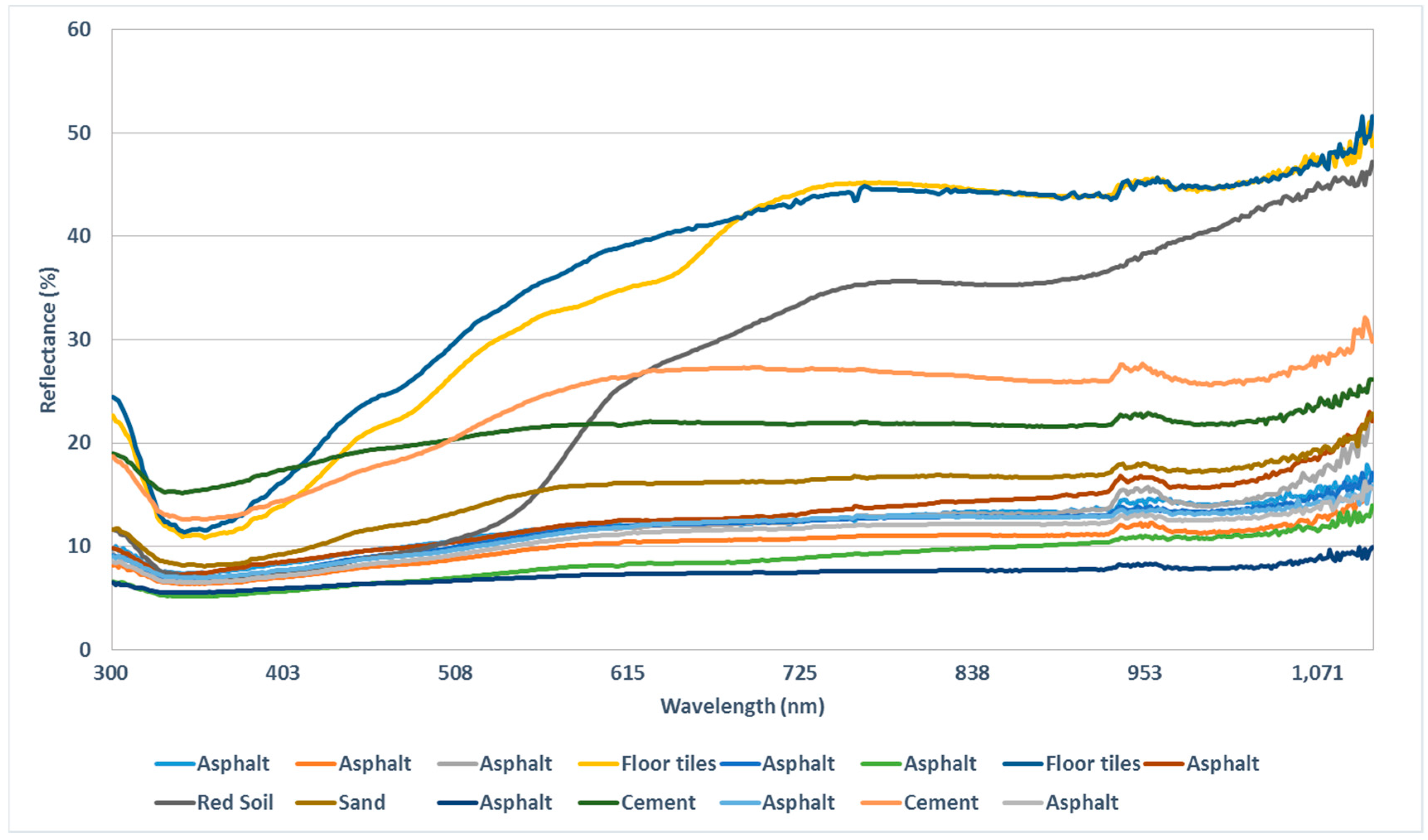
The Spectral Evolution PSR-1100 handheld spectroradiometer was employed to measure the bidirectional diffuse spectral reflectance from 299.6 to 1107.3 nm with a bandwidth of less than 2 nm, as shown in Figure 4. The PSR-1100 spectroradiometer was positioned at an average height of 60 cm above the target in the nadir position using a 250 angular field of view. The standard white reference panel Spectralon®, a barium sulfate plate, was used to measure the white reference spectra in each set of measurements. Note that at least 50 sample spectra were collected and averaged at each site. Instead of serving as the end members for mangrove classification, these spectra measured outside TNP are mainly used as the ground truths of surface reflectance for the validation of atmospheric correction.
2.2.2. Atmospheric Correction
Contaminated by the absorption and scattering effects of atmospheric particles, the spectral signals detected by the hyperspectral sensors mounted on the airborne or spaceborne platforms comprise noise from the atmosphere and signals from the land surface. To retrieve the subtle surface reflectance signal, atmospheric correction is the first process used to identify and separate the significant noise contributed by the atmosphere. Approaches to atmospheric correction fall into three rather broad categories: radiative transfer models, ground-based measurements, and dark object subtraction techniques [23]. Radiative transfer models, such as the MODTRAN-based (MODerate resolution atmospheric TRANsmission) Fast Line-of-sight Atmospheric Analysis of Hypercubes (FLAASH) model for EO-1 Hyperion data [4,10,15,16] and CASI data [14], as well as the ATCOR2 model for Landsat [22] and SPOT (French: Satellite Pour l’Observation de la Terre) data [25], are widely used for applications of hyperspectral imagery in mangrove-related research to remove atmospheric interference. They have been shown to significantly improve the accuracy of image classification. Because FLAASH provides well-adjusted inputs through derivation of atmospheric properties such as surface albedo, surface altitude, water vapor column and aerosol from the image [4], we followed the same procedure described in Held et al. [14] to extract the reflectance characteristics of the mangrove classes with the FLAASH model using commercial software (ENVI version 5.2). Parameters and options specified in FLAASH for atmospheric correction are listed in Table 1.
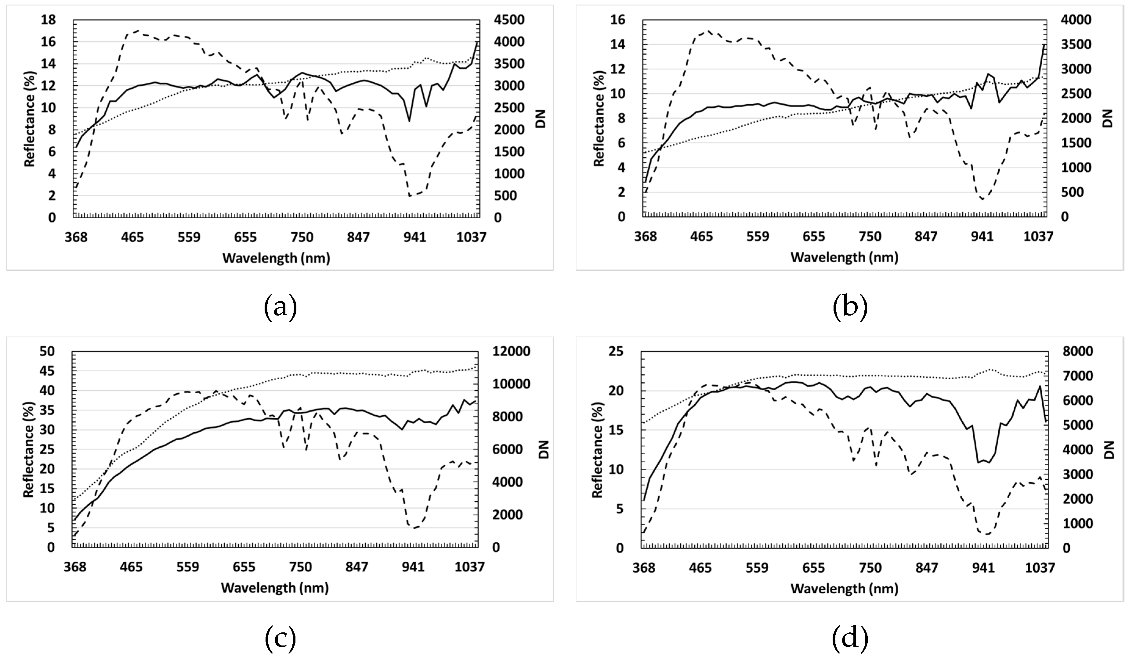
To evaluate the performance of FLAASH, the spectra measured at 15 sites outside TNP are compared to the spectra extracted from the FLAASH-corrected image, as shown in Figure 5. For the cases of asphalt (sites 1, 2, 3, 5, 6, 8, 11, 13, 15), both the trend and scale of surface reflectance between the ground measurements and the FLAASH-corrected spectra are rather consistent (Figure 5a,b). This demonstrates that the FLAASH is indeed able to correct the atmospheric interferences. For cases of floor tiles (sites 4 and 7) (Figure 5c), cement (sites 12 and 14) (Figure 5d), sand (site 10) (Figure 5e), and red soil (site 9) (Figure 5f), however, the deviations are apparent. The reason can be inferred from the field photographs of these sites. Figure 3c,d,e,f show that these sites are covered with large areas of artificial pavement, yet the small tiles and rugged surface of the red soil are not uniform from the point of view of the airborne CASI sensor. This comparison also highlights the influence of underlying wet soil and water on the spectral reflectance of wetland vegetation, as described by Heenkenda et al. [12]. Although the close-range hyperspectral reflectance of mangroves collected either in the laboratory or in the field can reveal not only the species level [18,19,20] but also the state of health and the nitrogen concentrations [21,22], these subtle signals will exhibit very different characteristics that need to be identified and extracted from the CASI imagery with special care.
2.3. Map of Mangrove Distribution
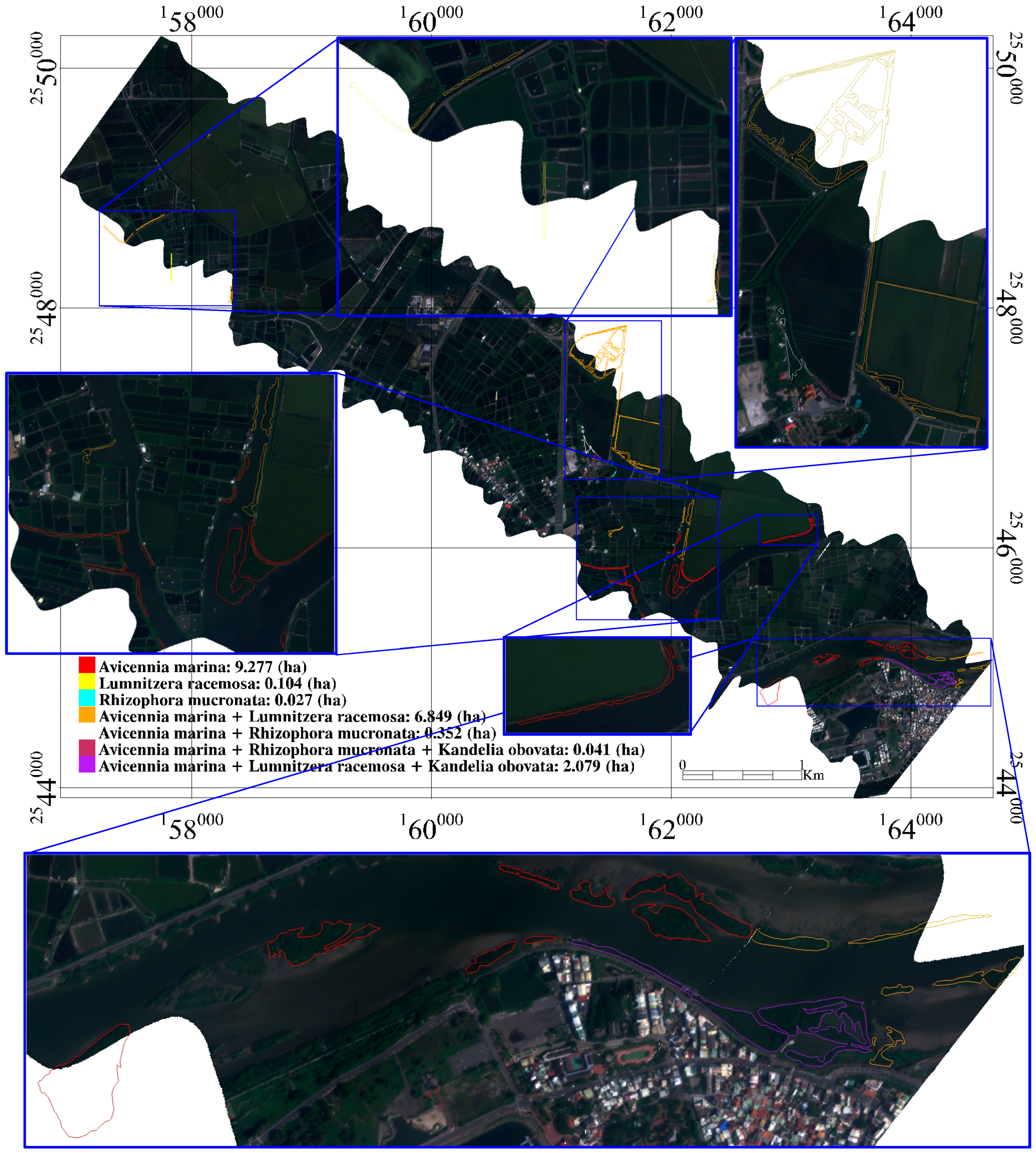
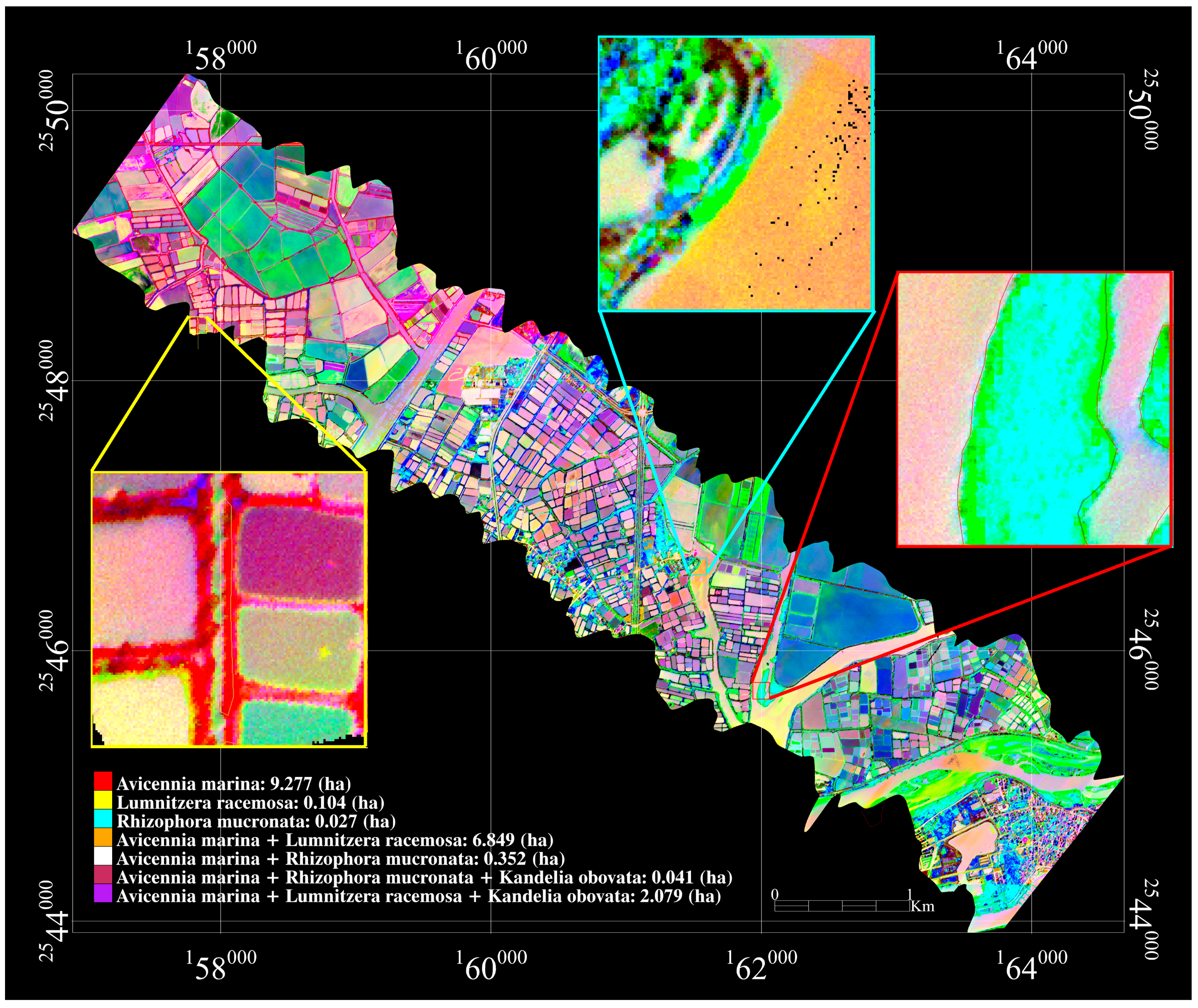
An overview of Taiwan’s mangroves, including diversity and distribution, uses, major threats, conservation and other problems was reported by Fan [26]. However, the detailed map of mangrove distribution was not available until the work by Wang et al. [27]. By means of in-depth interviews with experts and elderly local people, as well as aerial photographs comparison and literature review, they conducted a comprehensive field investigation at a total of 37 remnant habitats of mangrove in Taiwan in 2011 and produced a map of mangrove distribution. The three classes of pure mangroves and four classes of mixed mangroves derived from their field investigation are overlaid on the FLAASH-corrected imagery of TNP in Figure 6, with a legend showing both the species and area of each class. The areas of three pure mangroves, as shown as the red, yellow and cyan polygons in Figure 6, indicate that the most dominant species in TNP is Avicennia marina (9.277 ha), which is approximately 89.2 times of Lumnitzera racemosa (0.104 ha) and 343.6 times that of Rhizophora mucronata (0.027 ha). In addition, the total area of the three classes of pure mangroves (9.408 ha) is roughly the same as the total area of the four classes of mixed mangroves (9.321 ha). Since there is no pure class of Kandelia obovata that is rarely seen in TNP and mostly found in the northern part of Taiwan, we use the three classes of pure mangroves as the training area to identify the endmembers of pure mangrove, which plays a crucial role in the later analysis of CASI hyperspectral imagery.
2.4. Supervised Hourglass Hyperspectral Analysis
The core of hyperspectral data analysis is to identify endmember spectra that are spectrally unique and cannot be reconstructed as a linear combination of other image spectra. A variety of procedures have been developed to process hyperspectral imagery for classification. Kruse et al. [28] integrated a sequence of recommended operations and proposed an end-to-end analysis, namely the HHA approach, which has been implemented in various commercial software packages, such as ENVI® and Geomatica®. Odden [29] compared these two packages and concluded that ENVI® is a step ahead. However, the classification result is not satisfied by applying HHA directly to all of the CASI imagery because the spectral characteristics of the target mangroves and other trees/vegetation are too similar. We are not able, as a result, to identify the endmembers of pure mangrove, nor to determine their dynamic ranges of spectral variation for classification. In this research, therefore, we propose a supervised HHA by utilizing three classes of pure mangrove that were derived from the field investigation by Wang et al. [27] in 2011, as shown as the red, yellow and cyan polygons in Figure 6. These regions are regarded as training areas, within which the HHA is employed first to identify the endmembers of pure mangrove and determine their dynamic spectral variation ranges for the purpose of classification. This is analogous to the decision tree approach that predicts the value of a target variable by learning simple decision rules inferred from the data features [30].
2.4.1. Minimum Noise Fraction Transform
The first step of the HHA is to determine the inherent dimensionality of the hyperspectral imagery, which enables the identification of the number of spectrally distinguishable endmembers through the separation of a signal from noise. This task can be accomplished by performing a Minimum Noise Fraction (MNF) Transform, so the vast majority of unique spectral information will be contained within the first few MNF transform bands [31]. In other words, the number of spectral bands can be significantly reduced after this processing step.
As shown in Figure 2 and Figure 6, the strip that covers most of the training areas of known mangrove trees is selected first. The MNF transform is applied to the entire strip and only the training areas, respectively. Figure 7 displays a profile of the MNF eigenvalue, of which larger values contain signals and smaller ones contain noise. The eigenvalue falls dramatically after eigenvalue number 11 for the case of training areas only (solid line), and 20 for the case of the entire strip (broken line). Since the training areas are comprised of mangrove trees, the vast majority of unique spectral information is expected to be contained within a small number of MNF transform bands. However, the first 11 bands out of the entire 72 bands are still required to preserve most of the signal and variance. As will be revealed later, focusing on the training areas with known mangrove trees, indeed, preserves more signal and variance to discriminate different species of mangroves from the background.
2.4.2. Pixel Purity Index and Endmembers
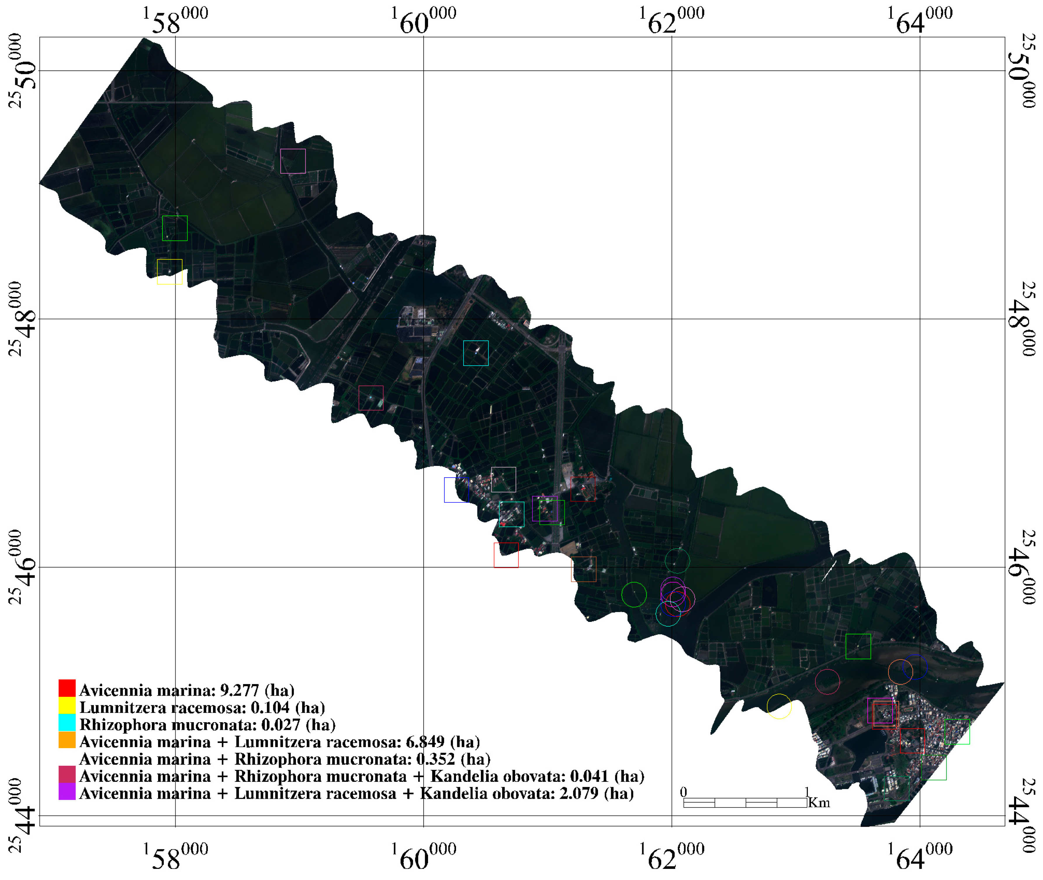
The second step of the HHA is to identify the pixels that are pure and obtain the endmembers. This task can be accomplished by creating a Pixel Purity Index (PPI) Image, on which each pixel value corresponds to the number of times that that pixel was recorded as extreme. Because the endmembers (pure pixels) will most likely only be represented by a few pixels, they do not occur with extreme frequency. This step reduces the data spatially so that it is possible to only focus on pixels that are pure. To retrieve endmembers from the MNF-inversed image on which the spectral bands have been significantly reduced, the n-D scatter plots are repeatedly projected onto a random unit vector, and the extreme pixels are counted in each projection. The PPI is calculated as the total number of times each pixel has been marked as extreme during the projection iteration. The spectra of endmembers are determined by those pixels with larger PPI values. The location of each endmember is labeled in Figure 8 as a colorful square box (entire strip) or a circle (training area only).
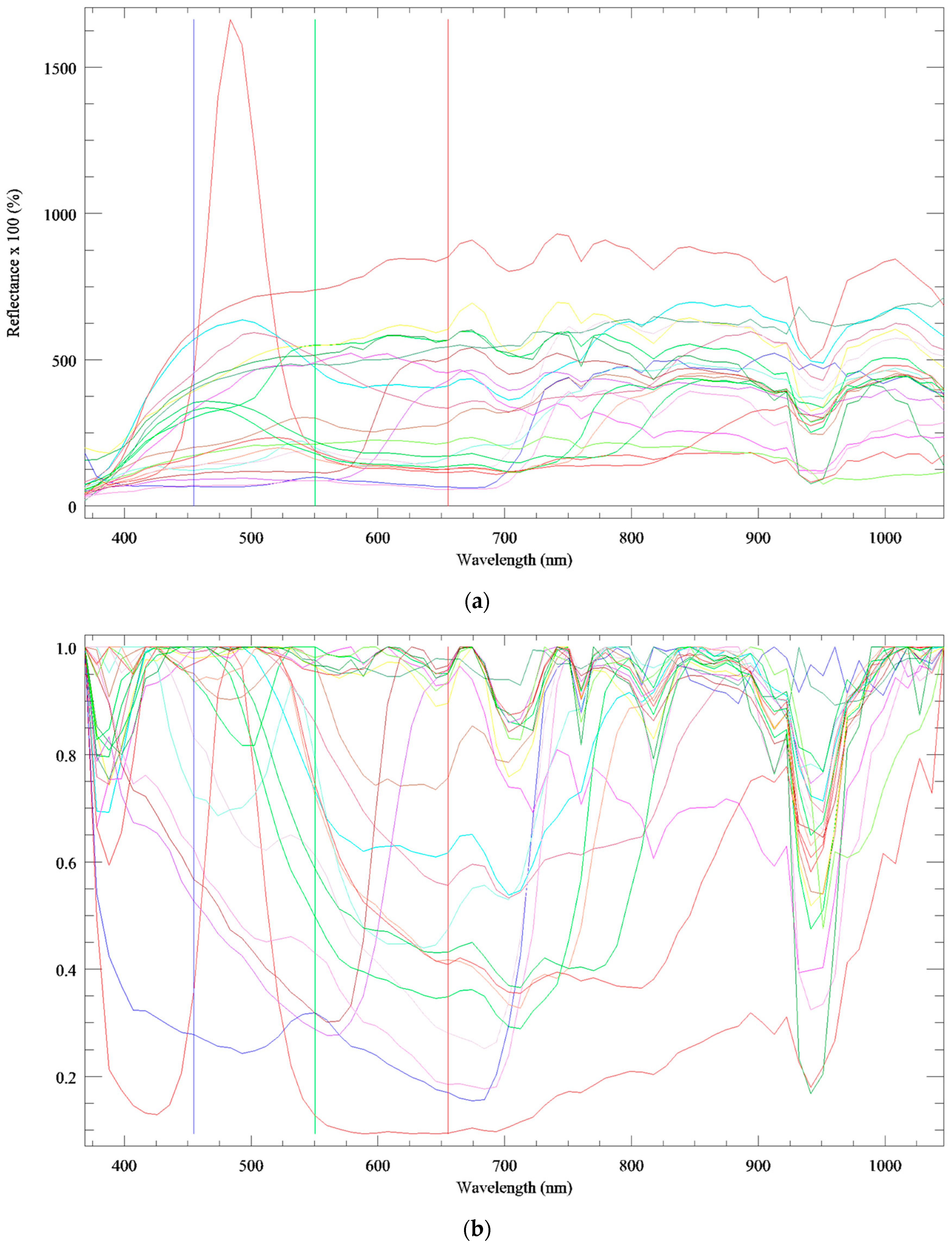
The spectra of the 21 endmembers for the case of the entire strip are shown in Figure 9a. Generally speaking, they exhibit rather different spectral characteristics. To normalize the reflectance spectra, we use continuum removal to compare individual absorption features from a common baseline, as shown in Figure 9b. The continuum fits over the top of a spectrum using straight-line segments that connect local spectra maxima [32,33,34]. This approach is ideal for identifying and highlighting the absorption features of hyperspectral data. However, no apparent features of absorption can be determined from Figure 9b. This can be better comprehended by taking a closer look at each pixel with its surrounding land use/land cover, which requires a higher spatial resolution to see the details.
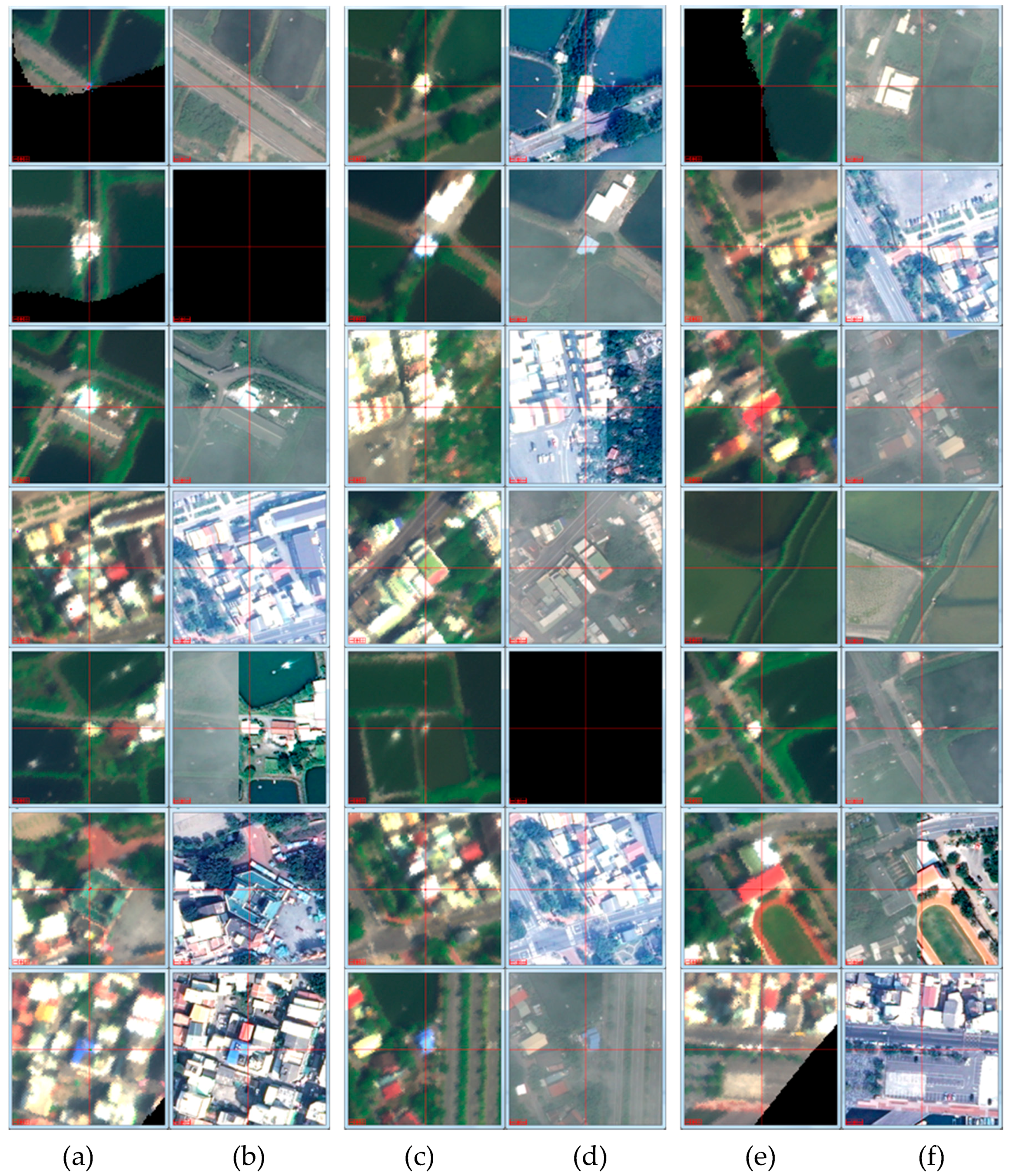
The Aerial Survey Office of the Forestry Bureau happened to acquire a set of high-spatial-resolution (25 cm) aerial photographs of TNP on October 19, 2013, just about one month after our acquisition of the CASI image. Under the assumption that no significant changes of land use/land cover occurred between these two dates of image acquisition, these orthophotographs serve as another source of data to provide more detailed spatial information and to verify our interpretations. Note that the CASI image resolution was resampled from 1 m to 25 cm (Figure 10a,c,e) in order to compare to the aerial photographs (Figure 10b,d,f). Most of the 21 endmembers shown in Figure 10 represent man-made objects, such as buildings, roads, pavements, or even cars. Only three of them show the vegetation pattern and none of them fall within the known areas of mangrove trees. In the case of one strip of CASI image taken over TNP that is mostly covered by vegetation, only a small region of the man-made objects dominated the spectral variation signal and caused the PPI to find more extreme pixels, rather than pure endmembers. These endmembers might be good for land use/land cover classification, but they provide limited information for mapping pure mangrove patches.
Although all three classes of pure mangroves are included in the training area (red, yellow and cyan polygons), Figure 8 shows that all 12 PPI-determined endmembers obtained from the case of the training area (colorful circles) are located in the class of Avicennia marina (red polygons). Note that the most dominant species in TNP is Avicennia marina (9.277 ha), which is approximately 89.2 times Lumnitzera racemosa (0.104 ha) and 343.6 times Rhizophora mucronata (0.027 ha). As a result, the endmembers of pure Lumnitzera racemosa and Rhizophora mucronata cannot be retrieved from the PPI image automatically. They need to be added to our analysis manually, based on the map of mangrove distribution derived from the field investigation by Wang et al. [27] in 2011.
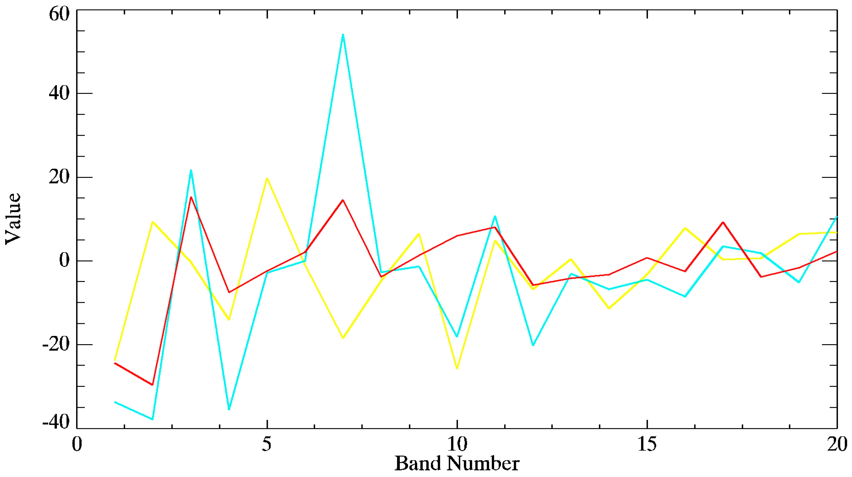
The spectra of the first 20 MNF bands collected at three pure pixels of Avicennia marina, Lumnitzera racemosa and Rhizophora mucronata are plotted and compared in Figure 11. Since the spectral reflectance among the three species of mangrove and other plants are rather similar in the original CASI hyperspectral image [19], it is difficult to locate mangroves by including the signals from these spectral bands. By carefully comparing the spectral characteristics among the three species of mangroves, we designate the MNF bands 2, 7, 10 as red, green and blue channels to make a false-color composite, as shown in Figure 12. This false-color composite made of the three characteristic bands enhances the subtle difference in spectral reflectance among the three species of mangrove and other plants.
Even within a well-defined training area with pure mangroves such as the red, cyan and yellow boxes enlarged in Figure 12, there are still some pixels dominated by the tree shadows or small water pits. As a result, they exhibit a relatively low, yet monotone pattern of the reflected spectrum. Taking the other factors such as underlying wet soil, water, the state of health and the nitrogen concentrations into consideration, it is not practical to expect to retrieve “pure” endmembers that are free from the influences of other factors. Nevertheless, by examining the spectral features illustrated by the MNF bands (Figure 11) and the false-color composite of the MNF-transformed image, the three endmembers retrieved from the training areas provide the required spectral characteristics to differentiate the three species of mangrove and other plants.
3. Results
Compared to the other approaches of supervised classification, the SAM approach is insensitive to illumination and albedo effects caused by shadows. This approach classifies each pixel by calculating the angle between the endmember spectrum vector and each pixel vector in n-D space [34]. Bearing in mind that TNP is basically wetlands covered with a lot of fish farms, salt pans, and river channels, the mangrove mainly grows in a narrow corridor along the water or in groups on a small sandbank. It is quite common to see one species of mangrove mingled with another species of mangrove, or even with other plants. Therefore, one pixel might cover different mangroves or plants. Instead of labeling each pixel to a certain class of mangrove, it makes more sense to present a set of SAM rule images corresponding to the spectral angle calculated between each pixel and each target (one rule image per target). A smaller spectral angle means that the pixel is a better match to the target. With the knowledge of three endmembers (Figure 11) and three training areas with three pure mangroves (enlarged boxes in Figure 12), the histogram of a rule image that contains the classification measures in units of radian (solid line in Figure 13) for each training area is shown in Figure 13a,c,e. As aforementioned, even within the training areas with pure mangroves, there are still some pixels dominated by the tree shadows or small water pits. As a result, they exhibit a relatively low, yet monotone pattern of reflected spectrum. We can assume that most parts of the training areas are pure mangrove and the rest part are non-mangrove pixels. Otsu’s method is then employed to determine the threshold for each mangrove species (dashed lines in Figure 13) to dichotomize the image into the mangrove and the non-mangrove pixels in each training area. The same threshold (Table 2) is applied to the entire strip to map the same mangrove species, as shown in Figure 13b,d,f.
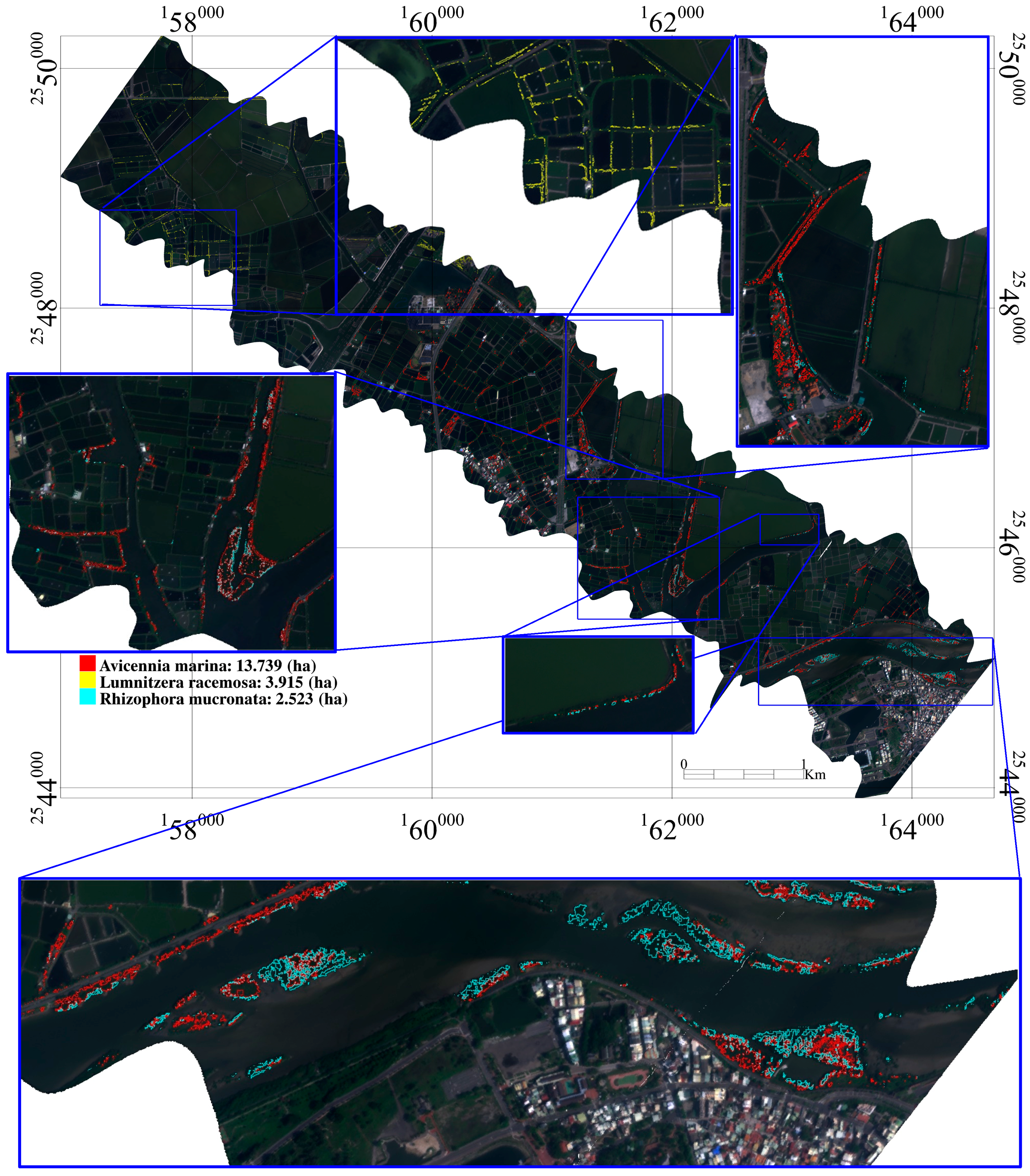
The CASI hyperspectral image derived map of the pure patches of Avicennia marina, Lumnitzera racemosa and Rhizophora stylosa is shown in Figure 14. This map, however, cannot be compared pixel-to-pixel with the map of mangrove distribution derived from the field investigation by Wang et al. [27] in 2011 (Figure 6). Because the SAM approach classifies each pixel according to its spectral similarity to the three endmembers, while the field investigation labels different regions with different species composition, even within one region labeled with one or two mangrove species, we can still identify some corresponding pixels in the CASI hyperspectral image that are actually contaminated by tree shadows, water pits, or mingled with other trees. In other words, the map of mangrove distribution derived from the field investigation is not meant to be used to validate the CASI hyperspectral image derived map of pure mangrove patches. Nevertheless, calculating the total area of each mangrove species from both maps indeed assists us to evaluate the result of classification, as listed in Table 3.
4. Discussion
TNP is basically a conserved and restricted wetland covered with a lot of fish farms, salt pans, and river channels. The major challenges of mapping mangroves with airborne hyperspectral imagery in TNP are the lack of ground truths measured from a field spectroradiometer mounted on a heavy truck, and the target mangroves are usually mingled with other plants in a narrow corridor along the water or in groups on a small sandbank. Hyperspectral imagery acquired from airborne or spaceborne platforms have been reported to discriminate [4], classify [15], or map the abundance and distribution of mangrove species [10,14], However, this mainly occurred in vast areas where a few mangrove species dominate. This work demonstrates that the MOD-TRAN-based FLAASH model can indeed correct the atmospheric interference to a certain level of accuracy for the cases of asphalt. However, for cases of floor tiles, cement, sand, and red soil with small tiles and rugged surface, the deviations are apparent. Not to mention the influence of underlying wet soil and water on the spectral reflectance of wetland vegetation. It is very unlikely to remove the atmospheric interference and retrieve the subtle signals of spectral characteristics to identify mangroves or other vegetations to the species level in TNP, at least with the CASI hyperspectral images that are currently available.
Although the number of spectral bands can be significantly reduced by the MNF transform, for discriminating various mangrove species with very similar spectral reflectance, it is better to select a few training areas with known mangrove trees first and then conduct the MNF transform in those areas only to determine the endmembers that are representative in order to target mangrove species. The standard HHA approach identifies the pixels that are pure and obtains the endmembers by creating a PPI Image. The PPI-derived spectra of 21 endmembers for the case of the entire strip exhibit rather different spectral characteristics. After comparing with the high-spatial-resolution (25 cm) aerial photographs, we found that most of the 21 endmembers represent man-made objects, such as buildings, roads, pavements, or even cars. Only three of them show the vegetation pattern, and none of them fall within the known areas of mangrove trees. These endmembers might be good for land use/land cover classification, but they provide limited information for mapping pure mangrove patches.
The map of mangrove distribution derived from the field investigation by Wang et al. [27] in 2011 assists us to determine the training areas with pure mangroves and exclude cases of mixed contribution. However, there are still some pixels dominated by the tree shadows or small water pits in the training areas. As a result, they exhibit a relatively low, yet monotone pattern of reflected spectrum. We make an assumption that most parts of the training areas are pure mangrove and the rest part are non-mangrove pixels. Otsu’s method is then employed to determine the threshold for each mangrove species to dichotomize the image into the mangrove and the non-mangrove pixels in each training area. The same threshold is applied to the entire strip to map the same mangrove species. Although the CASI-derived map cannot be compared pixel-to-pixel with the map of mangrove distribution derived from the field investigation by Wang et al. [27] in 2011 (Figure 6), the total area of each mangrove species calculated from both maps indeed assists us to evaluate the result of the classification.
The densely crisscrossed channels of brine in TNP created an ideal environment for mangroves to thrive, and all three major mangrove species can be found near water. Generally speaking, Avicennia marina is the most widely-spread species because of its special feature of an ascending respiratory root for mechanical fixation in loose soil and its ability to deal with low oxygen levels. Lumnitzera racemosa can tolerate more saline conditions than the other mangrove species, which makes it more advantageous in the regions regularly inundated by salt water and flushed out by fresh water. Rhizophora stylosa is the least frequent mangrove seen in Taiwan. Thanks to the Sicao Mangrove Preserve, there is a green tunnel formed by patches of mangroves along the drainage channels. Most of the Rhizophora stylosa are preserved well in the green tunnel. The total amount of Rhizophora stylosa is indeed much lower than the amount of Avicennia marina and Lumnitzera racemosa. Mapping the remnant Rhizophora stylosa patches, such as the regions revealed in Figure 14, is extremely important to the management of mangrove trees.
A remarkable feature of a “mangrove desert” is revealed on the north-western part of Figure 14. This area is covered by vegetation and the environment is supposed to be the same as the environment of TNP as well. However, our analysis of the CASI hyperspectral imagery indicated that very few signs of mangroves can be detected in this area. As a matter of fact, TNP was established in late 2009 when the consensus was that the rights and interests of local residents should be of higher priority. Some private lands are too expensive or even not allowed to be included in TNP. As a result, the scope of the TNP is rather fragmented (as delineated by the red lines in Figure 1), and regulation cannot be enforced outside of it. Quite a lot of mangroves outside TNP have disappeared for many reasons. Figure 14 illustrates the difference between protected and non-protected results, which highlights the fact that biodiversity can be easily and quickly destroyed if no protection is provided.
One limitation was the inability to collect ground truths, we were only able to visually identify the species of mangroves and other plants and estimate the amount of each species at this particular site. Considering the accuracy of position and the possible errors incurred by estimating the fraction of species from the ground, we can only use pure endmembers to map pure pixels with higher confidence. No reliable information on mangrove species and abundance for mixed pixels could be derived. To fully exploit the advantages of hyperspectral observation, however, the ratio of each endmember should be calculated for every pixel. This requires an efficient and objective approach to collect the ground truths of mangrove species and abundance for validation. Thanks to the advances in unmanned aerial vehicles (UAVs), it is now possible to plan a flight route and take a series of close-up photographs near the ground using a multi-axis drone [24]. With such high-spatial-resolution imagery, future works are planned to select good timing when certain types of mangroves are in blossom. Their flowers can be used as another useful characteristic for identifying mangrove species and coverage from a high-spatial-resolution photograph.
5. Conclusions
This work demonstrates that airborne CASI hyperspectral imagery can assist in mapping pure mangrove patches, even in a conserved and restricted wetland where the target mangroves are mingled with other plants in a narrow corridor along the water or in groups on a small sandbank. The key element of success is the detailed map of mangrove distribution derived from the field investigation, which enables us to determine the training areas with pure mangroves and exclude cases of mixed contribution. The MOD-TRAN-based FLAASH model can indeed correct the atmospheric interference to a certain degree of accuracy so that most of the major spectral characteristics are retrieved for hyperspectral analysis. For cases of non-uniform surfaces, however, the deviation between the ground measurements and the FLAASH-corrected spectra is apparent. This highlights the influence of underlying wet soil and water on the spectral reflectance of wetland vegetation. Therefore, instead of using close-range hyperspectral reflectance of mangroves collected either in the laboratory or in the field, it is more representative to use endmembers extracted directly from the CASI imagery. To make the best use of hyperspectral information for discriminating various mangrove species with very similar spectral reflectance, it is better to select a few training areas with known mangrove trees first and then conduct the MNF transform in those areas only to determine the endmembers that are representative of the target mangrove species. An operable approach is proposed to determine a unique threshold value for each pure endmember in the training area, which enabled the mapping of three major mangrove patches in TNP. The total areas of mangroves calculated from the map derived from the CASI hyperspectral image are consistent with the ones calculated from the map derived from the field investigation. The development of a “mangrove desert” highlights the fact that biodiversity can be easily and quickly destroyed if no protection is provided. Some remnant patches located in this research are extremely important to the management of mangrove trees. Future works are planned to enhance the collection of ground truths by employing a UAV to acquire hyperspectral photographs with high-spatial-resolution when certain types of mangroves are in blossom so that their flowers can be used to identify the mangrove species and their coverage. Such information will be crucial for deriving the mangrove species and abundance for every pixel, which truly manifests the advantages of hyperspectral observation.
Author Contributions
Conceptualization, C.-C.L.; Data curation, T.-W.H. and H.-L.W.; Formal analysis, H.-L.W. and K.-H.W.; Funding acquisition, C.-C.L.; Investigation, C.-C.L., T.-W.H. and H.-L.W.; Methodology, C.-C.L.; Project administration, C.-C.L.; Resources, C.-C.L.; Supervision, C.-C.L.; Validation, T.-W.H. and H.-L.W.; Visualization, H.-L.W.; Writing—original draft, C.-C.L.; Writing—review & editing, C.-C.L.
Funding
This research was supported by the Ministry of Science and Technology of Taiwan under Contract Nos. MoST 107-2611-M-006-002, and Taijiang National Park under Contract No. TNP-105-C19.
Acknowledgments
The authors acknowledge support from Hsiang-Hua Wang and Shu-Wei Fu in providing the map of mangrove distribution derived from the field investigation. We thank three anonymous reviewers for providing helpful comments on improving and clarifying this manuscript.
Conflicts of Interest
The authors declare no conflict of interest.
References
- Rey, J.R. Mangroves. In Environmental Geology; Springer: Berlin, Germany, 1999; pp. 396–397. [Google Scholar]
- Godoy, M.D.P.; Lacerda, L.D.D. Mangroves response to climate change: A review of recent findings on mangrove extension and distribution. An. Da Acad. Bras. De Ciências 2015, 87, 651–667. [Google Scholar] [CrossRef]
- Kuenzer, C.; Bluemel, A.; Gebhardt, S.; Quoc, T.V.; Dech, S. Remote sensing of mangrove ecosystems: A review. Remote Sens. 2011, 3, 878–928. [Google Scholar] [CrossRef]
- Koedsin, W.; Vaiphasa, C. Discrimination of tropical mangroves at the species level with EO-1 hyperion data. Remote Sens. 2013, 5, 3562–3582. [Google Scholar] [CrossRef]
- Food and Agriculture Organization of the United Nations. The World’s Mangroves, 1980–2005: A Thematic Study in the Framework of the Global Forest Resources Assessment 2005; Food and Agriculture Organization of the United Nations: Roma, Italy, 2007. [Google Scholar]
- Lee, T.-M.; Yeh, H.-C. Applying remote sensing techniques to monitor shifting wetland vegetation: A case study of danshui river estuary mangrove communities, taiwan. Ecol. Eng. 2009, 35, 487–496. [Google Scholar] [CrossRef]
- Polidoro, B.A.; Carpenter, K.E.; Collins, L.; Duke, N.C.; Ellison, A.M.; Ellison, J.C.; Farnsworth, E.J.; Fernando, E.S.; Kathiresan, K.; Koedam, N.E. The loss of species: Mangrove extinction risk and geographic areas of global concern. PLoS ONE 2010, 5, e10095. [Google Scholar] [CrossRef] [PubMed]
- Green, E.P.; Clark, C.D.; Mumby, P.J.; Edwards, A.J.; Ellis, A. Remote sensing techniques for mangrove mapping. Int. J. Remote Sens. 1998, 19, 935–956. [Google Scholar] [CrossRef] [Green Version]
- Pham, T.D.; Yokoya, N.; Bui, D.T.; Yoshino, K.; Friess, D.A. Remote sensing approaches for monitoring mangrove species, structure, and biomass: Opportunities and challenges. Remote Sens. 2019, 11, 230. [Google Scholar] [CrossRef]
- Giri, S.; Mukhopadhyay, A.; Hazra, S.; Mukherjee, S.; Roy, D.; Ghosh, S.; Ghosh, T.; Mitra, D. A study on abundance and distribution of mangrove species in indian sundarban using remote sensing technique. J. Coast. Conserv. 2014, 18, 359–367. [Google Scholar] [CrossRef]
- Fromard, F.; Vega, C.; Proisy, C. Half a century of dynamic coastal change affecting mangrove shorelines of french guiana. A case study based on remote sensing data analyses and field surveys. Mar. Geol. 2004, 208, 265–280. [Google Scholar] [CrossRef]
- Heenkenda, M.; Joyce, K.; Maier, S.; Bartolo, R. Mangrove species identification: Comparing worldview-2 with aerial photographs. Remote Sens. 2014, 6, 6064–6088. [Google Scholar] [CrossRef]
- Xia, Q.; Qin, C.-Z.; Li, H.; Huang, C.; Su, F.-Z. Mapping mangrove forests based on multi-tidal high-resolution satellite imagery. Remote Sens. 2018, 10, 1343. [Google Scholar] [CrossRef]
- Held, A.; Ticehurst, C.; Lymburner, L.; Williams, N. High resolution mapping of tropical mangrove ecosystems using hyperspectral and radar remote sensing. Int. J. Remote Sens. 2003, 24, 2739–2759. [Google Scholar] [CrossRef]
- Kumar, T.; Panigrahy, S.; Kumar, P.; Parihar, J. Classification of floristic composition of mangrove forests using hyperspectral data: Case study of bhitarkanika national park, india. J. Coast. Conserv. 2013, 17, 121–132. [Google Scholar] [CrossRef]
- Goenaga, M.A.; Torres-Madronero, M.C.; Velez-Reyes, M.; Van Bloem, S.J.; Chinea, J.D. Unmixing analysis of a time series of hyperion images over the guánica dry forest in puerto rico. IEEE J. Sel. Top. Appl. Earth Obs. Remote Sens. 2013, 6, 329–338. [Google Scholar] [CrossRef]
- Navarro, J.A.; Algeet, N.; Fernández-Landa, A.; Esteban, J.; Rodríguez-Noriega, P.; Guillén-Climent, M.L. Integration of uav, sentinel-1, and sentinel-2 data for mangrove plantation aboveground biomass monitoring in senegal. Remote Sens. 2019, 11, 77. [Google Scholar] [CrossRef]
- Prasad, K.A.; Gnanappazham, L.; Selvam, V.; Ramasubramanian, R.; Kar, C.S. Developing a spectral library of mangrove species of indian east coast using field spectroscopy. Geocarto Int. 2014, 30, 580–599. [Google Scholar] [CrossRef]
- Vaiphasa, C.; Skidmore, A.K.; de Boer, W.F.; Vaiphasa, T. A hyperspectral band selector for plant species discrimination. ISPRS J. Photogramm. Remote Sens. 2007, 62, 225–235. [Google Scholar] [CrossRef]
- Zhang, C.; Kovacs, J.; Liu, Y.; Flores-Verdugo, F.; Flores-de-Santiago, F. Separating mangrove species and conditions using laboratory hyperspectral data: A case study of a degraded mangrove forest of the mexican pacific. Remote Sens. 2014, 6, 11673–11688. [Google Scholar] [CrossRef]
- Zhang, C.; Kovacs, J.; Wachowiak, M.; Flores-Verdugo, F. Relationship between hyperspectral measurements and mangrove leaf nitrogen concentrations. Remote Sens. 2013, 5, 891–908. [Google Scholar] [CrossRef]
- Lagomasino, D.; Price, R.M.; Whitman, D.; Campbell, P.K.E.; Melesse, A. Estimating major ion and nutrient concentrations in mangrove estuaries in everglades national park using leaf and satellite reflectance. Remote Sens. Environ. 2014, 154, 202–218. [Google Scholar] [CrossRef]
- Campbell, J.B.; Wynne, R.H. Introduction to Remote Sensing, 5th ed.; Guilford Publications: New York, NY, USA, 2011; p. 667. [Google Scholar]
- Liu, C.-C.; Chen, Y.-H.; Wen, H.-L. Supporting the annual international black-faced spoonbill census with a low-cost unmanned aerial vehicle. Ecol. Inform. 2015, 30, 170–178. [Google Scholar] [CrossRef]
- Vo, Q.; Oppelt, N.; Leinenkugel, P.; Kuenzer, C. Remote sensing in mapping mangrove ecosystems—An object-based approach. Remote Sens. 2013, 5, 183–201. [Google Scholar] [CrossRef]
- Fan, K.-C. La mangrove de taiwan. Bois For. Des Trop. 2002, 273, 43–54. [Google Scholar]
- Wang, H.-H.; Fu, S.-W.; Teng, K.-C.; Hong, X.; Liao, H.-Y. Current status of mangrove area change and species composition in taiwan. Taiwan For. J. 2015, 41, 47–51. (In Chinese) [Google Scholar]
- Kruse, F.A.; Boardman, J.W.; Huntington, J.F. Comparison of airborne hyperspectral data and eo-1 hyperion for mineral mapping. IEEE Trans. Geosci. Remote Sens. 2003, 41, 1388–1400. [Google Scholar] [CrossRef] [Green Version]
- Odden, B. Comparison of a Hyperspectral Classification Method Implemented in Different Remote Sensing Software Packages. Ph.D. Thesis, University of Zurich, Zürich, Switzerland, 2008. [Google Scholar]
- Breiman, L.; Friedman, J.; Stone, C.J.; Olshen, R.A. Classification and Regression Trees; CRC Press: Boca Raton, FL, USA, 1984. [Google Scholar]
- Boardman, J.W. Automating Spectral Unmixing of Aviris Data Using Convex Geometry Concepts; NASA: Washington, DC, USA, 1993.
- Clark, R.N.; Roush, T.L. Reflectance spectroscopy: Quantitative analysis techniques for remote sensing applications. J. Geophys. Res. Solid Earth 1984, 89, 6329–6340. [Google Scholar] [CrossRef]
- Green, A.; Craig, M. Analysis of Aircraft Spectrometer Data with Logarithmic Residuals; NASA: Washington, DC, USA, 1985.
- Kruse, F.; Lefkoff, A.; Boardman, J.; Heidebrecht, K.; Shapiro, A.; Barloon, P.; Goetz, A. The spectral image processing system (SIPS)—Interactive visualization and analysis of imaging spectrometer data. Remote Sens. Environ. 1993, 44, 145–163. [Google Scholar] [CrossRef]
Figure 1.
The geographical location of Taijiang National Park (TNP) (delineated by red lines) and the four main wetland areas: Zengwen Estuary Wetland, Sicao Wetland, Qigu Salt Pan Wetland and Yanshui Estuary Wetland. Our study area is located in the main part of TNP, covering Yanshui Estuary Wetland and Sicao Wetland. The true color image (10 m resolution) was acquired by Sentinel-2 on 15 February 2018.

Figure 2.
The color composite of five strips of hyperspectral images with a spatial resolution of 1 m that covered 25 km2, taken with the ITRES CASI 1500 at an altitude of 1000 m on 9 September 2013. The CASI scanner flight route is denoted as the dotted line. The Greenwich Mean Time (GMT) time of each pass is listed. The locations of 15 sites of ground measurements are labeled as fuchsia dots and yellow numbers.

Figure 3.
The field photographs of the 15 sites: (1) Asphalt, (2) Asphalt, (3) Asphalt, (4) Floor tiles, (5) Asphalt, (6) Asphalt, (7) Floor tiles, (8) Asphalt, (9) Red soil, (10) Sand, (11) Asphalt, (12) Cement, (13) Asphalt, (14) Cement, (15) Asphalt.
Figure 3.
The field photographs of the 15 sites: (1) Asphalt, (2) Asphalt, (3) Asphalt, (4) Floor tiles, (5) Asphalt, (6) Asphalt, (7) Floor tiles, (8) Asphalt, (9) Red soil, (10) Sand, (11) Asphalt, (12) Cement, (13) Asphalt, (14) Cement, (15) Asphalt.

Figure 4.
The bidirectional diffuse spectral reflectance measured with the Spectral Evolution PSR-1100 handheld spectroradiometer at 15 sites outside TNP, of which the locations are denoted in Figure 2 and the images of which are provided in Figure 3.

Figure 5.
The comparison of the spectra measured at 15 sites outside TNP (dotted lines), the spectra extracted from the CASI imagery (broken lines), and the FLAASH-corrected imagery (solid lines). The cases of (a) site 1: asphalt, (b) site 6: asphalt, (c) site 7: floor tiles, (d) site 12: cement, (e) site 10: sand, and (f) site 9: red soil.


Figure 6.
The map of mangrove distribution derived from the field investigation by Wang et al. [27] in 2011. Three classes of pure mangroves and four classes of mixed mangroves are overlaid on the FLAASH-corrected imagery of TNP with a legend showing both the species and area of each class. The five regions annotated by blue boxes are enlarged to clearly show the mangrove patches.

Figure 7.
The profile of the Minimum Noise Fraction (MNF) Eigenvalues for the case of the entire strip (broken line) and the case of training areas only (solid line).
Figure 7.
The profile of the Minimum Noise Fraction (MNF) Eigenvalues for the case of the entire strip (broken line) and the case of training areas only (solid line).

Figure 8.
The locations of endmembers determined by calculating the Pixel Purity Index (PPI) from the MNF-inversed image. The 21 colorful square boxes were obtained from the case of an entire strip and the 12 colorful circles were obtained from the case of the training area only.
Figure 8.
The locations of endmembers determined by calculating the Pixel Purity Index (PPI) from the MNF-inversed image. The 21 colorful square boxes were obtained from the case of an entire strip and the 12 colorful circles were obtained from the case of the training area only.

Figure 9.
The spectra of (a) reflectance, and (b) normalized reflectance for the 21 endmembers retrieved from the MNF-inversed full strip image.
Figure 9.
The spectra of (a) reflectance, and (b) normalized reflectance for the 21 endmembers retrieved from the MNF-inversed full strip image.

Figure 10.
The comparison of the CASI image (a,c,e) and the aerial orthophotograph (b,d,f) for the 21 endmembers retrieved from the MNF-inversed full strip image.
Figure 10.
The comparison of the CASI image (a,c,e) and the aerial orthophotograph (b,d,f) for the 21 endmembers retrieved from the MNF-inversed full strip image.

Figure 11.
The spectra of the first 20 MNF bands collected at three pure pixels (annotated in Figure 12) of Avicennia marina (red), Lumnitzera racemosa (yellow) and Rhizophora mucronata (cyan). The spectral difference among the three species of mangroves is most apparent at bands 2, 7 and 10, which are, therefore, designated as the red, green and blue channels to make a false-color composite, as annotated by the three vertical red, green and blue lines.

Figure 12.
The false-color composite of the MNF-transformed image by designating the MNF bands 2, 7, 10 as the red, green and blue channels. Three endmembers are collected at the center pixels of three training areas with pure mangroves, including Avicennia marina (red box), Lumnitzera racemosa (yellow box) and Rhizophora mucronata (cyan box), as plotted and compared in Figure 11.

Figure 13.
The histogram (solid line) of a rule image that contains the classification measures in units of radian for each training area: (a) Avicennia marina, (c) Rhizophora stylosa and (e) Lumnitzera racemosa; and for the entire strip: (b) Avicennia marina, (d) Rhizophora stylosa and (f) Lumnitzera racemosa. The threshold (dashed line) for each mangrove species is determined by Otsu’s method to dichotomize the image into the mangrove and the non-mangrove pixels in each training area. The same threshold is applied to the entire strip to map the same mangrove species.

Figure 14.
The CASI hyperspectral image derived map of the pure patches of Avicennia marina (red polygon), Lumnitzera racemosa (yellow polygon) and Rhizophora mucronata (cyan polygon) in TNP. The five regions annotated by blue boxes (the same as shown as Figure 6) are enlarged to clearly show the mangrove patches.


Table 1.
The parameters and options specified in Fast Line-of-sight Atmospheric Analysis of Hypercubes (FLAASH) for atmospheric correction.
Table 1.
The parameters and options specified in Fast Line-of-sight Atmospheric Analysis of Hypercubes (FLAASH) for atmospheric correction.
| Parameters/Options | Values/Settings |
|---|---|
| Sensor Type | CASI |
| Scene Center location | (23.0 N, 121.0 E) |
| Sensor Altitude | 2 km |
| Ground Elevation | 0.0 km |
| Pixel Size | 1 m |
| Flight Date | 9 September 2013 |
| Flight Time GMT | 0:44:57 |
| Atmospheric Model | Tropical |
| Aerosol Model | Rural |
| Spectral Polishing | Yes |
| Water Retrieval | Yes |
| Aerosol Retrieval | None |
| Width (number of bands) | 9 |
| Water Absorption Feature | 940 nm |
| Initial visibility | 40 km |
| Wavelength Recalibration | No |
| Aerosol Scale Height | 2.0 km |
| CO2 Mixing Ratio | 390.0 ppm |
| Use Square Slit Function | Yes |
| Use Adjacency Correction | Yes |
| Reuse MODTRAN Calculations | No |
| Modtran Resolution | 15 cm−1 |
| Modtran Multiscatter Model | Scaled DISORT |
| Number of DISORT Streams | 8 |
Table 2.
The threshold value of each endmember determined by the histogram of a rule image.
| Mangrove | Avicennia marina | Rhizophora stylosa | Lumnitzera racemosa |
|---|---|---|---|
| Threshold (radian) | 0.605 | 0.498 | 0.614 |
Table 3.
The total area of mangroves calculated from the map derived from the CASI hyperspectral image (Figure 14) and the map derived from the field investigation by Wang et al. [27] (Figure 6).
| Mangrove | Avicennia marina + Lumnitzera racemosa | Avicennia marina + Rhizophora stylosa | |
|---|---|---|---|
| Source | |||
| Map derived from the field investigation by Wang et al. [27] | 18.309 (ha) | 9.695 (ha) | |
| Map derived from the CASI hyperspectral image | 17.654 (ha) | 16.262 (ha) | |
© 2019 by the authors. Licensee MDPI, Basel, Switzerland. This article is an open access article distributed under the terms and conditions of the Creative Commons Attribution (CC BY) license (http://creativecommons.org/licenses/by/4.0/).
Share and Cite
MDPI and ACS Style
Liu, C.-C.; Hsu, T.-W.; Wen, H.-L.; Wang, K.-H. Mapping Pure Mangrove Patches in Small Corridors and Sandbanks Using Airborne Hyperspectral Imagery. Remote Sens. 2019, 11, 592. https://0-doi-org.brum.beds.ac.uk/10.3390/rs11050592
AMA Style
Liu C-C, Hsu T-W, Wen H-L, Wang K-H. Mapping Pure Mangrove Patches in Small Corridors and Sandbanks Using Airborne Hyperspectral Imagery. Remote Sensing. 2019; 11(5):592. https://0-doi-org.brum.beds.ac.uk/10.3390/rs11050592
Chicago/Turabian StyleLiu, Cheng-Chien, Tsai-Wen Hsu, Hui-Lin Wen, and Kung-Hwa Wang. 2019. "Mapping Pure Mangrove Patches in Small Corridors and Sandbanks Using Airborne Hyperspectral Imagery" Remote Sensing 11, no. 5: 592. https://0-doi-org.brum.beds.ac.uk/10.3390/rs11050592
Note that from the first issue of 2016, this journal uses article numbers instead of page numbers. See further details here.