Processing Chain for Estimation of Tree Diameter from GNSS-IMU-Based Mobile Laser Scanning Data


1
Department of forest management and geodesy, Faculty of Forestry, Technical University in Zvolen, T. G. Masaryka 24, 96053 Zvolen, Slovak Republic
2
Faculty of Forestry and Wood Sciences, Czech University of Life Sciences Prague, 16500 Praha 6, Suchdol, Czech Republic
*
Authors to whom correspondence should be addressed.
Remote Sens. 2019, 11(6), 615; https://0-doi-org.brum.beds.ac.uk/10.3390/rs11060615
Submission received: 29 January 2019
/
Revised: 7 March 2019
/
Accepted: 11 March 2019
/
Published: 13 March 2019
(This article belongs to the Special Issue 3D Point Clouds in Forests)
Abstract
:Mobile laser scanning (MLS) is a progressive technology that has already demonstrated its ability to provide highly accurate measurements of road networks. Mobile innovation of the laser scanning has also found its use in forest mapping over the last decade. In most cases, existing methods for forest data acquisition using MLS result in misaligned scenes of the forest, scanned from different views appearing in one point cloud. These difficulties are caused mainly by forest canopy blocking the global navigation satellite system (GNSS) signal and limited access to the forest. In this study, we propose an approach to the processing of MLS data of forest scanned from different views with two mobile laser scanners under heavy canopy. Data from two scanners, as part of the mobile mapping system (MMS) Riegl VMX-250, were acquired by scanning from five parallel skid trails that are connected to the forest road. Misaligned scenes of the forest acquired from different views were successfully extracted from the raw MLS point cloud using GNSS time based clustering. At first, point clouds with correctly aligned sets of ground points were generated using this method. The loss of points after the clustering amounted to 33.48%. Extracted point clouds were then reduced to 1.15 m thick horizontal slices, and tree stems were detected. Point clusters from individual stems were grouped based on the diameter and mean GNSS time of the cluster acquisition. Horizontal overlap was calculated for the clusters from individual stems, and sufficiently overlapping clusters were aligned using the OPALS ICP module. An average misalignment of 7.2 mm was observed for the aligned point clusters. A 5-cm thick horizontal slice of the aligned point cloud was used for estimation of the stem diameter at breast height (DBH). DBH was estimated using a simple circle-fitting method with a root-mean-square error of 3.06 cm. The methods presented in this study have the potential to process MLS data acquired under heavy forest canopy with any commercial MMS.
1. Introduction
Mobile laser scanning (MLS) is the latest technology within geospatial data acquisition that enables time-efficient measurements of any ground-based object with high accuracy. The latest commercial mobile mapping systems (MMS) can acquire data on the road in a short time with an accuracy comparable to the total station measurements [1,2,3,4,5]. The range accuracy of mobile laser scanners contained in these systems spans from 2 mm (ROADSCANNER) to 50 mm (DYNASCAN) according to Puente et al. [6]. Employing one of these systems in forest measurements can be highly beneficial for the extraction of forest structural parameters at the tree level. The positioning of this existing solution, however, depends on the global navigation satellite system (GNSS) signal with varying strengths in the forest environment. Measurements of objects using systems from the 2010s with an GNSS outage duration of 1 min were tested in the study of Puente et al. [6]. These systems were able to measure the x- and y-positions with an accuracy ranging from 0.1 m (VMX-250/LYNX, ROADSCANNER) to 0.265 m (IP-S2 AG60), while the z-position was measured with an accuracy ranging from 0.07 m (VMX-250/LYNX, ROADSCANNER) to 0.24 m (IP-S2 AG60) [6].
Generally, two approaches to the positioning of MMS are applied for forest mapping. Primarily, the GNSS-inertial measurement unit (IMU) integrated system is used for this purpose [7,8,9]. The location of a point cloud generated using data from GNSS-IMU can then be improved using an optimized pose graph obtained from graph-based simultaneous localization and mapping (GraphSLAM) without additional measurements of the distance between MMS and tree stems [10,11]. Secondly, the location relative to the starting point of the MMS survey is recorded by a positioning system integrating IMU and SLAM [11,12,13,14,15,16]. SLAM has been garnering interest in recent studies [10,11,12,13,14,15,16]. In the study of Tang et al., the GNSS was substituted by improved maximum likelihood estimation (IMLE) based SLAM [13]. The authors reported that the IMLE-based SLAM solution of forest mapping can produce an accurate stem map for forests with symmetric stems. On the other hand, the IMLE-based SLAM solution fails to provide accurate positioning in open areas. Furthermore, 2D scans of the forest positioned by the SLAM/IMU system can be used for forest mapping [16]. Extended Kalman filter (EKF) based SLAM algorithm was used for the purpose of forest mapping in Forsman et al. [16]. The SLAM/IMU system is also used for positioning in handheld mobile laser scanning (HMLS) [12,14,16].
The use of vehicle-based MLS for forest mapping has been demonstrated in previous studies [7,9,13,15,17,18,19,20]. The pilot studies investigated the use of MLS for tree diameter estimation in areas with sufficient GNSS signal [17,18,19]. These conditions are typical for urban forests. Moreover, studies show that high accuracy in both tree location and diameter at breast height (DBH) estimates can be achieved using MLS [18,19]. Nevertheless, processing of data acquired by MLS under heavy forest canopy is a challenging task. Outages in GNSS signal cause errors in MMS trajectory location. This leads to multiple copies of objects that appear in the MLS point cloud, generated using the erroneous trajectory each time the objects are scanned. The quality of personal laser scanning data (PLS) acquired under heavy forest canopy was compared with the quality of airborne laser scanning data (ALS) scanned from an unmanned aerial vehicle (UAV) by Rönnholm et al. [9]. The authors reported average initial misalignment between the two data sets of 0.227, 0.073, and −0.083 m in the easting, northing, and elevation directions, respectively. Such misalignments can result in inaccurate estimations of tree position and diameter.
In order to align the MLS data acquired from different views under heavy forest canopy, the iterative closest point (ICP) algorithm can be used [9]. The basic ICP algorithm was introduced by Chen and Medioni [21] and Besl and McKay [22]. Latest software for point cloud data processing offers point cloud registration based on the basic ICP algorithm [23,24,25]. This algorithm requires rough initial registration of the point clouds and is able to align only one transformed point cloud to one reference point cloud. The rough registration does not represent a problem for the registration of misaligned MLS point clouds, since it can be provided by GNSS-IMU [9]. The ICP algorithm was used in the study of Rönnholm et al. [9] to align PLS data to reference ALS data scanned from the UAV [9]. By employing the ICP algorithm, Rönnholm et al. reported a decrease in the previously mentioned average misalignment between the PLS data and the ALS data from UAV to 0.084, 0.020, and −0.005 m, in the easting, northing, and elevation directions, respectively. The ICP algorithm, which was recently integrated into the modular program system OPALS, is able to align multiple transformed point clouds to one reference [25]. The algorithm was initially proposed for the adjustment of airborne laser scanning strips, where it was able to improve the relative orientation of the pre-processed strips (defined as standard deviation of the residual point-to-plane distances for all strip to strip correspondences) from 1.83 cm to 1.38 cm [26]. Consequently, this algorithm has great potential for aligning MLS point clouds scanned from different views under heavy forest canopy.
Estimation of DBH from MLS data using various methods was demonstrated in numerous studies [7,8,11,12,14,15,16,19]. These studies report the accuracy of DBH estimation from MLS data comparable to terrestrial laser scanning (TLS). Liang et al. [27] concluded this similarity for forest stands with stem densities of ∼600 trees/ha. Highly promising results of DBH estimation were achieved using handheld laser scanners [12,14,16]. These scanners can provide relatively accurate stem maps, and the acquisition is much less time-consuming compared to TLS. On the other hand, increased occurrence of point noise was reported in the handheld mobile laser scanning (HMLS) point cloud compared to the TLS point cloud [12,14]. HMLS also has a shorter working range (10–30 m) and lower accuracy (3 cm) than vehicle-based MLS [12,14,16].
Most commercial MMS are positioned by the GNSS-IMU system. These systems represent a highly available and time-effective solution for forest mapping. In this study, the MLS data was acquired using a commercial MMS—Riegl VMX-250 mounted on a tractor. The data from MMS was already processed for the purposes of tree diameter estimation, and some results were published in Čerňava et al. [20]. It is obvious that the MLS provides a high level of automation for the acquisition of data from the forest on a tree level. The aim of this study is to propose the processing chain for registration of point clusters from tree stems scanned from different views and consequent estimation of tree diameters from the aligned data. By proposing the optimal processing chain, we aim to decrease the degree of interference needed for extraction, matching, and registration of the misaligned MLS data from the tree stems scanned from different views under heavy forest canopy.
The processing chain presented in this paper combines the method for DBH estimation introduced by Koreň et al. [28] with processing in OPALS [29,30,31]. In addition, we introduce a method for extraction of the misaligned scenes of forest contained in the MLS point cloud, generated using data from IMU, GNSS, and an external odometer. The extraction of the misaligned scenes in form of individual point clouds is performed using the GNSS time based spatial clustering program in Python. The extracted point clouds are then reduced to 1.15-m thick horizontal slices, and for each slice, trees are detected using the Group by distance method [28]. Point clusters representing tree stems scanned from multiple views, which were extracted from individual horizontal slices, are grouped based on their correspondence to the same tree stem. For each group of point clusters, the horizontal overlap is calculated. Sufficiently overlapping point clusters from the individual tree stem are aligned with the ICP algorithm proposed by Glira et al. [25]. Points at height ranging from 1.275 m to 1.325 m are used for DBH estimation using Monte Carlo method introduced by Koreň et al. [28]. Koreň et al. achieved an accuracy of 2.38 m in the DBH estimation from single-scan TLS data using the Monte Carlo method. The authors also report the accuracy of DBH estimation from multi-scan TLS data at 0.77 cm.
2. Materials and Methods
2.1. Study Site
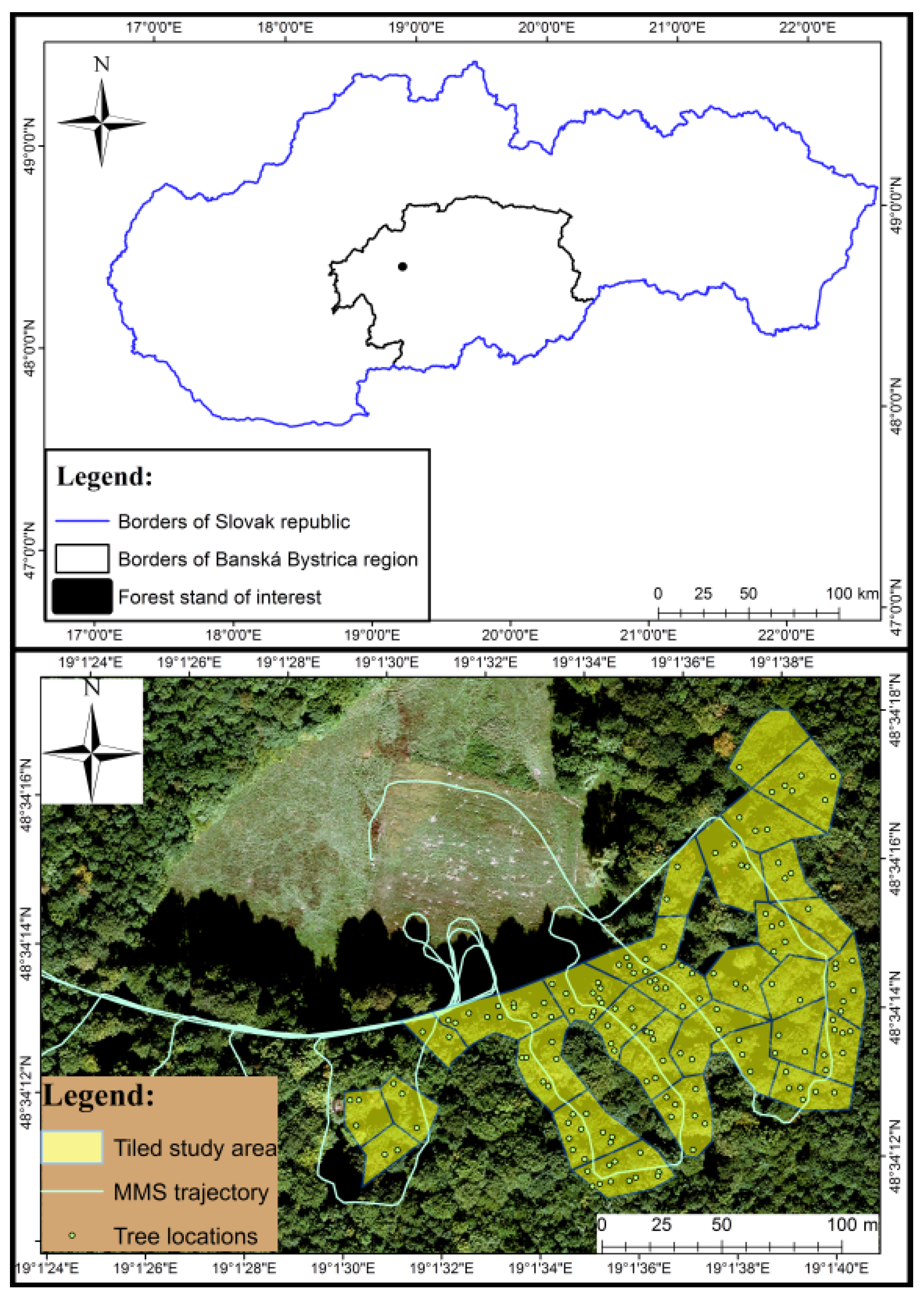
The study site with a total area of 1.58 ha is located in Budča, Banská Bystrica region, central Slovakia (Figure 1) (48°34′12.286″ N, 19°1′30.415″ E). The study site contains a 110-year-old forest stand of beech (Fagus sylvatica L.) (83%), oak (Quercus petraea L.) (10%), and hornbeam (Carpinus betulus L.) (7%). The forest stand is managed by the Forest Enterprise of the Technical University in Zvolen. The DBH for trees located on the study site ranges from 0.1 m to 0.8 m. The forest stand has a relative density of 0.7 and absolute stem density of 181 trees/ha. The main forest road is located at the northern part of the study site. Furthermore, skid trails leading south into the forest are connected to the forest road.
The condition of the terrain located under the forest canopy was classified based on the system presented by Simanov et al. [32]. In this system, the terrain belongs to the most accessible class, which allowed the use of tractors as a platform for mounting the MMS.
2.2. Mobile Mapping System
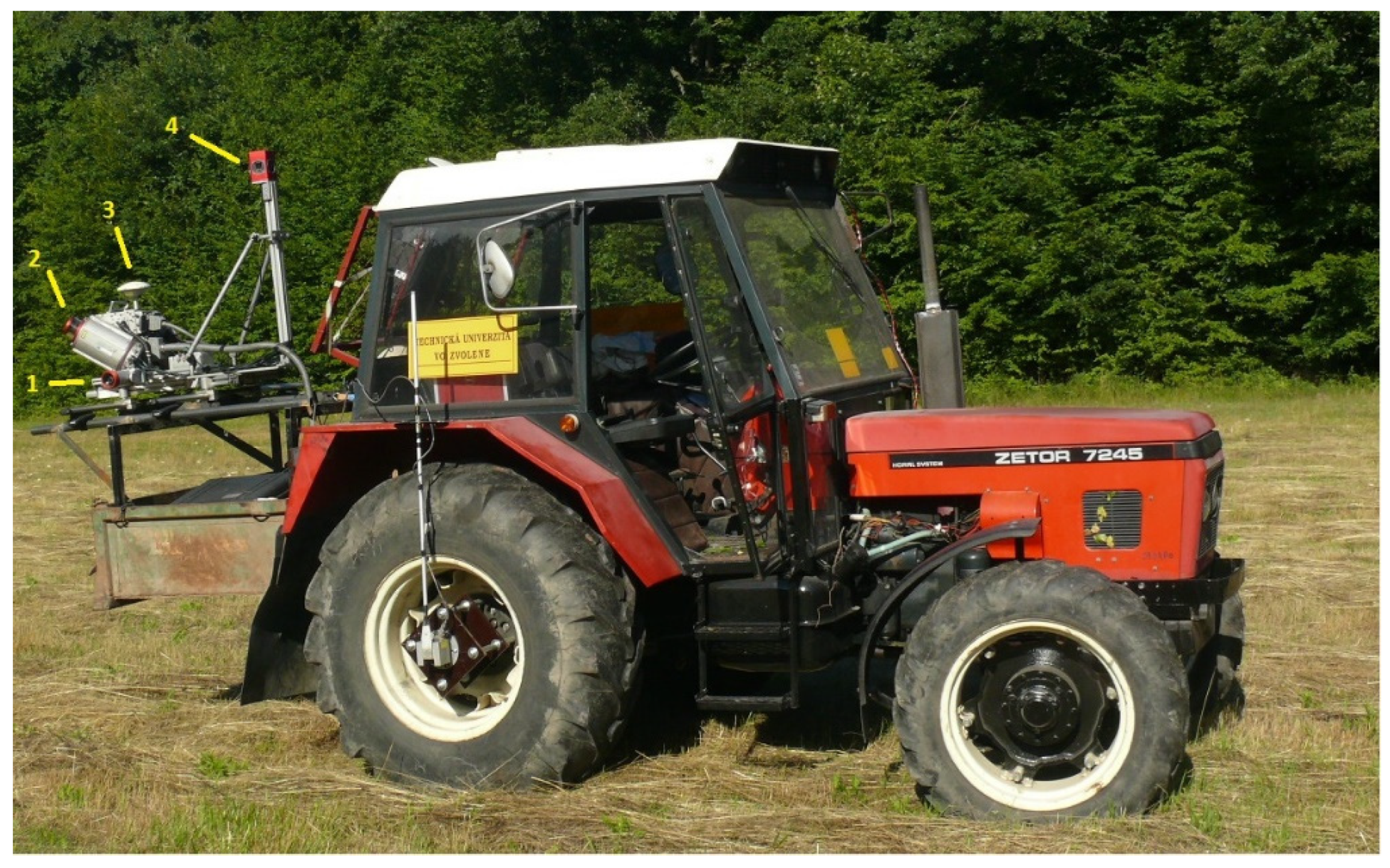
The MMS used to perform the study was Riegl VMX-250 (RIEGL Laser Measurement Systems GmbH, Horn, Austria) (Figure 2), which includes two integrated mobile laser scanners VQ-250, one panoramic camera and two additional digital cameras with high resolution (2452 × 2056 pixels). This study is focused on the processing of data obtained from these mobile laser scanners.
The MMS navigation system consisted of the Applanix GNSS-POS LV 510, IMU-31, odometer, and control unit. The Applanix GNSS-IMU navigation system, integrated on the RIEGL VMX-250, is only suitable for outages up to 1 min/1 km [33]. The MMS was mounted on tractor Zetor Horal 7245 (Zetor Tractors a. s., Brno, Czech Republic). Table 1 and Table 2 list further details and technical specifications of the MMS.
2.3. Mobile Laser Scanning Data
The MMS survey was conducted in July 2015. The survey started and ended in the open forest area. Static GNSS measurements of MMS position were carried out before and after the survey. The scanner VQ-250, included in the MMS, offers three settings of effective measurement rates. During the survey, the measurement rate was set to 600 kHz (300 kHz for each scanner). This measurement rate is intended for medium range applications. The maximal measurement range using this frequency is 200 m. Laser scanners were placed at approximately 1.8 m height, using the entire field of view (360°) for mapping. MMS was moved throughout the study site mostly at walking speed, or slower during maneuvering at the edges of the study site.
The tractor size limited the mapping to the forest road and skid trails throughout the forest. Nevertheless, because the density of the forest road network is high, much of the forest stand was mapped from the roads. The mean density for the point clouds acquired at the study site using both VQ-250 scanners was 31,301 points per square meter.
2.4. Reference Data
Reference data on 154 trees were collected in December 2015 using caliper with scale resolution of 1 mm. The majority of the reference sample is collected from trees located not further than 15 m from skid trails or the forest road, to ensure easier tree detection at the point cloud cross-section. Up to the 15 m from the road and skid trails, all of the trees were measured during the field works. Furthermore, several trees located outside the 15 m mark in areas with low stem density were also measured. Diameters at breast height (DBH) were measured at 1.3 m height in two perpendicular directions. The 1.3 m height was determined by measuring tape individually for each measurement. Locations of DBH measurements were adapted to the terrain. First DBH measurements were collected along the terrain contour line, and the second collection was perpendicular to the first direction of measurement. The mean of these two values was used as the reference DBH value. A stem map was created during the reference data collection. In the map, the relative position of the tree stems and the distance between the tree stem and the forest road or skid trail were marked.
Reference data were imported into ArcGIS 10.2 on a tree-by-tree basis, using point cloud cross-section and the stem map. The geometry of the forest road and skid trails was then used to assign a reference value to each point cluster from the tree stem visible on the point cloud cross-section. In most cases, the tree stems were found using the recorded distance between the stem and the forest road or skid trail. In addition, the distance between the tree stems and stem diameter was also considered when assigning of reference values to a point cluster.
2.5. Data Processing
2.5.1. Pre-Processing of Mobile Mapping System Data
The MMS trajectory was calculated with the Applanix POSPac software using differential GNSS data. GNSS reference data were acquired from the reference station installed on the roof of the main building of TU Zvolen (6.76 km from the study site). Positions of trajectory parts from periods with GNSS outage were corrected using data from IMU and odometers. These periods have a direct influence on the position and elevation error of MMS data.
The calculated trajectory was imported into RiPROCESS software. In this software, the MLS point cloud was generated and consequently georeferenced. The generated point cloud was saved in LAS 1.2 format.
Data exported from RiPROCESS was imported into the modular program system OPALS. In OPALS, the two point clouds from scanner 1 and scanner 2 were divided into smaller subsets of points using geometric information of 30 tiles defined as polygons in ArcGIS 10.2 (Figure 1). Initially, the plots were intended to reduce the processing time of a very dense point cloud. A horizontal slice of the raw point cloud from one scanner was visualized in ArcMap, and each boundary was created so that no tree stem is located at the plot boundary. The relative areas of the sample plots were also similar. Smaller point clouds were then processed individually.
2.5.2. GNSS Time-Based Point Clustering
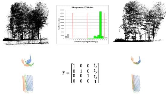
Upon investigation of the horizontal slice of the point cloud from scanner 1, we observed copies of individual tree stems appearing in the slice. Moreover, these copies were intersecting, and it was not possible to separate them using geometric information of the cluster (Figure 3). Therefore, GNSS time was used for separation of intersecting clusters.
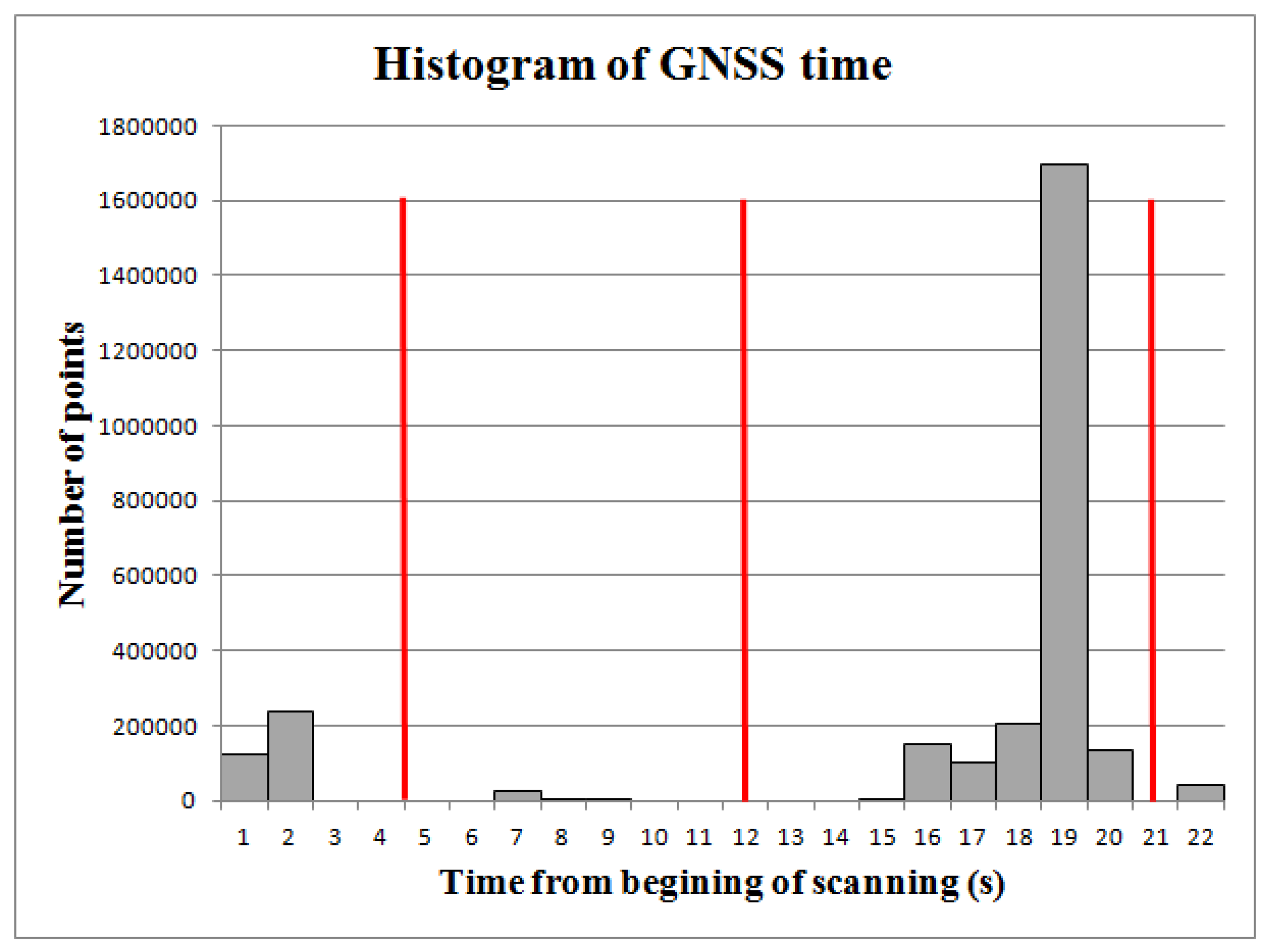
The histogram of GNSS time was created for each pre-processed point cloud from a sample plot. The histogram bin-width used for the processing was set individually for every point cloud. The bin width ranged from 0.001 s to 36.1 s. MLS data were then divided using the resulting gaps in the histogram. Gaps were defined by the bins in the histogram that did not contain any points. The GNSS time value of the gap center was used for division (Figure 4). A subset of points extracted from the point cloud was saved only if it comprised more than 10,000 points. Smaller subsets contained usually sets of ground points that were too sparse, which could cause erroneous calculations of normalized height for the point cloud. The subsets of points were saved as individual point clouds.
2.5.3. Extraction of Tree Stems
Point clouds extracted using GNSS time-based clustering were imported into the OPALS system. Ground points were classified using the lasground application, which forms part of the software package LAStools [34]. This software uses the triangulated irregular network (TIN) for classification of ground points. Sets of points classified as ground points in the LAStools software usually do not contain points reflected from higher vegetation or branches. This helps avoid interpolation of the digital terrain model (DTM) with extreme values.
Ground points were imported into OPALS and DTMs with a resolution of 2.5 m, and they were interpolated by simple snapping of the nearest elevation point and assigning it to a cell. Normalized height was calculated as the difference in elevation of each point and the nearest DTM cell.
In the last step, the horizontal slice of point cloud was generated by extracting the points with normalized height ranging from 0.35 m to 1.5 m. A slice of points from the tree stem located at lower heights was chosen to improve ICP-based alignment of the point cluster. The point clouds from lower parts of the tree stems are more complex. Therefore, by including of lower part of the stem for registration, the number of false correspondences for aligned point clusters can be decreased.
Point clusters from tree stems were extracted using Group by distance method (Koreň et al., 2017). Points are clustered together with the search for the nearest neighbor in 2D Euclidean space. The point cluster from the tree stem is defined by the maximum distance between the points of the cluster and the minimum number of points contained in the cluster. Points were clustered using maximum 5 cm inter-point distance, and only clusters consisting of more than 100 points were considered as tree stems. Point clusters from individual tree stems were saved as individual files.
The generated LAS files were visually inspected and point clusters from non-tree objects were removed. If point cluster from tree stem contained excessive point noise from branches or undergrowth, the noise was manually removed using LASview [34].
2.5.4. Matching of Point Clusters from Individual Tree Stems
Point clusters from both scanners were compared using three parameters for 30 sample plots. All possible combinations of point cluster pairs were compared with respect to the three parameters. The first parameter was the 2D distance between the centroids of compared clusters distAB. This parameter was used mostly to reduce the redundancy of compared data.
The second parameter, used for comparison of point clusters, was the index of duplicity id. This coefficient was calculated as
where is the mean GNSS time, is the mean of x coordinates, and is the mean of y coordinates, for point cluster A. The same definition of parameters applies to point cluster B.
This parameter was proposed based on the fact that copies of the same tree stem scanned from different views appeared in the point cloud near each other (dAB ≤ 1.5 m). Meanwhile, the period of time, during which the same tree stem was scanned twice, is much longer than time required for scanning of two neighboring tree stems. Therefore, point clusters with the higher value of id (20–3000) are most likely misaligned duplications of the same tree stem scanned from different views.
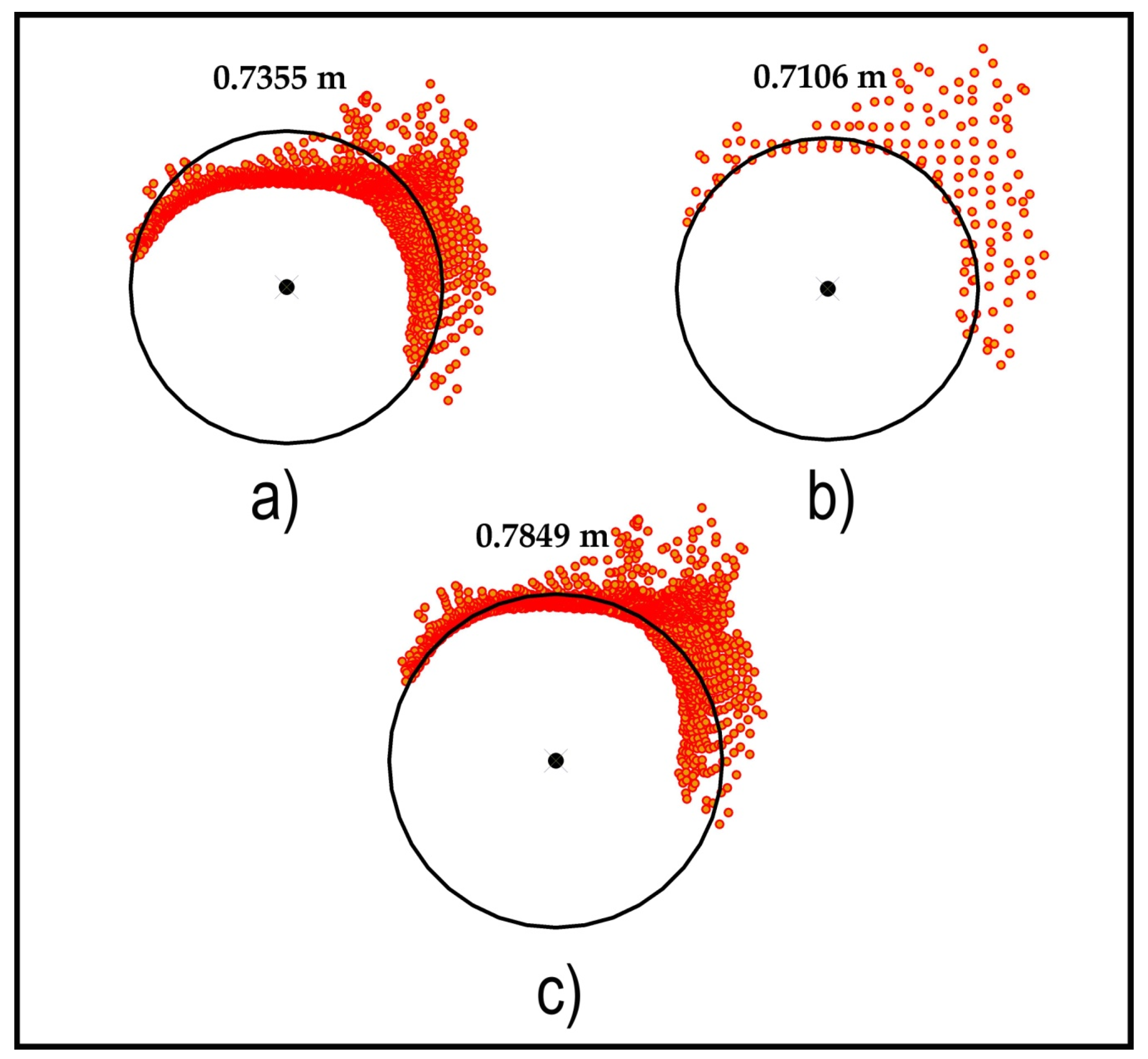
The third parameter, used for comparison of point clusters, was the difference between the estimated diameters of compared point clusters ∆dAB. The diameter was estimated using a simple circle-fitting method. The initial circle center was estimated by the midpoint of the line connecting two most distant points of the cluster (Figure 5a). Subsequently, the position of the circle center was shifted into four directions (+x, −x, +y, −y) by 5 mm steps, and for each new circle position, the radius ro that best fits the point cluster is found by minimizing the RMSE, calculated as
where r is the radius of the estimated circle, and ri is the Euclidian distance between the point of the cluster and the center of the circle.
The new circle center is then shifted to the position with lowest RMSE, and the ro found for the new position is used as the radius of the new circle. If the RMSE of all new circle centers and ro is higher than the RMSE from the previous iteration, the current position of the circle center is chosen as a final solution. The circle center is first estimated using the generalized geometry of the point cluster. The geometry was obtained by reducing the number of points of the cluster using a regular 4-cm grid. Only points that are nearest to the grid cell centers are selected for circle-fitting (Figure 5b). The best circle for the generalized cluster geometry is estimated by changing the circle center with corresponding ro in 200 iterations. Finally, circle parameters are optimized using all points in the cluster in 20 iterations (Figure 5c).
The thresholds of these three parameters were set empirically, and compared files containing point clusters A and B were labeled as copies of the same tree stem in the case where distAB < 1.5 m, idAB > 9, and ∆dAB < 0.15 m (stem0000_0001 and stem0001_0000).
2.5.5. Registration of Point Clusters from Individual Tree Stems
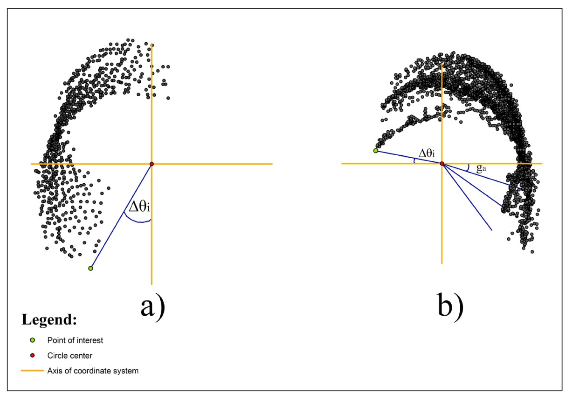
Previously labeled files with point clusters from tree stems were imported into the OPALS system. Registration of the clusters was carried out in Pyscripter environment. Before the registration, the horizontal overlap of point clusters was calculated. This was done to avoid termination of the registration due to lack of overlap for the point clusters from the same tree stem. To calculate the overlap, direction angles of all points were calculated for every compared point cluster. The point cluster was divided into four zones with a range of 90° using the previously estimated center of the point cluster and four additional points pointing to each cardinal direction (Figure 6). The additional points were located at 3/5 of the point cluster diameter from the point cluster center. The zero-direction angle was defined by the point directed to the east. The direction angle is then increased counterclockwise. The direction of the point ∆θi is calculated using a triangle. The triangle is defined by the point directed towards the cardinal direction with a direction angle θc of 0°/360°, 90°, 180°, and 270°, which is the nearest to the point of interest, center of the point cluster and the point of interest (Figure 6a). First, the difference between the direction of the point and direction of the nearest point of the cardinal direction is calculated as
where distc,i is the distance between the center of the point cluster and the point i, distc,a is the distance between the center of the point cluster and the nearest point of cardinal direction, and disti,a is the distance between the point i and the nearest point of cardinal direction. The arccosine was calculated using the math library for Python 2.7.
After solving Equation (3), the second nearest point of the cardinal direction is found. Based on the two nearest points of the cardinal direction, the calculated difference value of angle ∆θi is transformed into the direction angle. The direction is calculated either by adding or by subtracting the value of direction angle θn of the nearest point of the cardinal direction. If the direction angle θn+1 of the second the nearest point of cardinal direction is higher than direction angle θn of the nearest one, the direction angle of the nearest point θn of the cardinal direction is added to the difference of angle ∆θi. Otherwise, the difference of angle ∆θi is subtracted from the direction angle θn of the nearest point of the cardinal direction.
After calculating the direction angle for each point in the cluster, the range of the angles is calculated. In the first step of the angle calculation, the maximal angle gap is calculated as
where ro is the best radius for the circle with the lowest RMSE found using Equation (2), and distGBD is the maximal distance between the points of the cluster used for the detection of tree stems using the Group by distance method (Figure 6b).
There are two different approaches to the angle range calculation. If any point in the cluster has a direction angle of 0 ± ga°, the histogram of direction angles is created. The histogram bin-width is ga°. The number of points for the bins in the histogram are checked, starting from the bin with direction angles ranging from 360° to 360 - ga°, until a bin with no points is found. The minimum value of the direction angle is taken as the start of the angle range from last bin containing any number of points. The maximum angle of all the points with angles lower than the starting value of the angle range is considered as the angle at the end of the angle range (Figure 6b). If no point in the cluster has a direction angle of 0 ± ga°, a simple calculation of the angle range is used. In this case, the minimum value of the direction angle is used as the start of the angle range, and the maximum value is used as the end of the angle range (Figure 6a). Finally, calculated angle ranges for compared point clusters are used to estimate the horizontal overlap of the point clusters intended for registration. If their overlap is higher than 55°, point clusters proceed to registration.
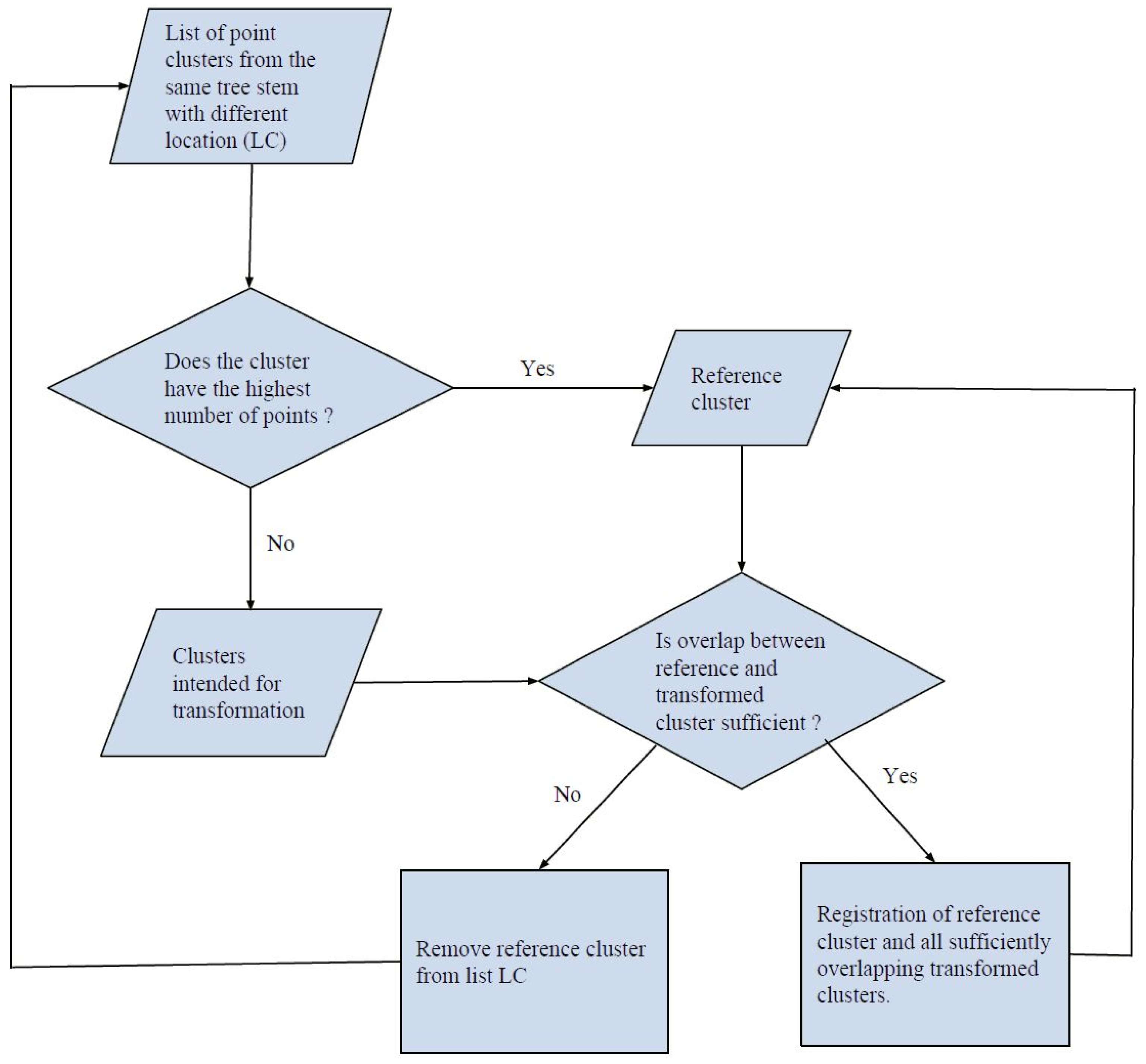
Registration of copies represented by point clusters from individual tree stems was carried out using the OPALS ICP module. The module aligns point clouds using the ICP method, a point to plane algorithm introduced by Glira et al. [25]. Point clusters from the individual stem were located near to each other, such that rough registration of the clusters was not necessary. This rough registration was obtained by the MMS trajectory based georeferencing of the MLS data. The registration was implemented in Pyscripter. First, point clusters were grouped based on their correspondence to a tree stem (based on the name of the file containing point cluster). The point cluster with the highest number of points in a group was set as a fixed reference, and the overlap of point clusters from the individual stem was subsequently calculated group-wise. The remaining point clusters were aligned to the reference cluster. The registration consists of five main steps, as described by Glira et al. [25]:
I. Finding the Overlap
The overlapping area of the point clusters is determined by so-called voxel hulls. Voxel hulls are a low resolution representation of the volume occupied by the point clusters [25]. For the computation of the voxel hull, the object space was subdivided into a voxel structure constructed by voxels with the edge length of 1 m.
II. Selection
In this step, a subset of points in the overlapping area of each transformed point cluster was initially selected by uniform sampling with a distance of 1 cm. The number of uniformly sampled points was then reduced using normal space sampling. The aim of this strategy is to select points such that the distribution of their normals in angular space is as uniform as possible [30]. The percentage of points used for the reduction was set manually during the registration and varied based on the overlap of the point cluster intended for registration.
III. Matching
The corresponding points (nearest neighbor) of the selected subset were found in the reference point cluster.
IV. Rejection
False correspondences (outliers) are rejected on the basis of the compatibility of points. In this study, the correspondences were rejected if:
- Maximum roughness of fitted planes was higher than 0.15 and 0.4 for noise-free and noisy point clusters, respectively.
- Maximum angle deviations between the normals of focal neighborhoods was higher than 15° or 40° for noise-free and noisy point clusters, respectively.
Furthermore, the parameter of maximal Euclidean distance between the correspondences was set to 5 m. Therefore, no correspondences were rejected based on distance.
V. Weighting
In this step, a weight (0 ≤ ω ≤ 1) was assigned to each correspondence.
The weight value depends on the roughness attribute of corresponding points and the angle between the normals of corresponding points.
VI. Minimization
Transformation parameters were estimated for the transformed point clusters by minimizing the squared distances between the corresponding points. The point-to-plane distance of two corresponding points is defined as the orthogonal distance of one point to the fitted plane of the other point. All points within a sphere of the specified search radius are considered for the plane fitting. In this study, the search radius varied based on the size of the point cluster and the point density of the cluster. In this step, a transformation matrix is calculated in the form
where tx is the x-axis shift, ty is the y-axis shift, and tz is the z-axis shift. The matrix shows that no rotation was calculated for the transformed point cloud.
VII. Transformation
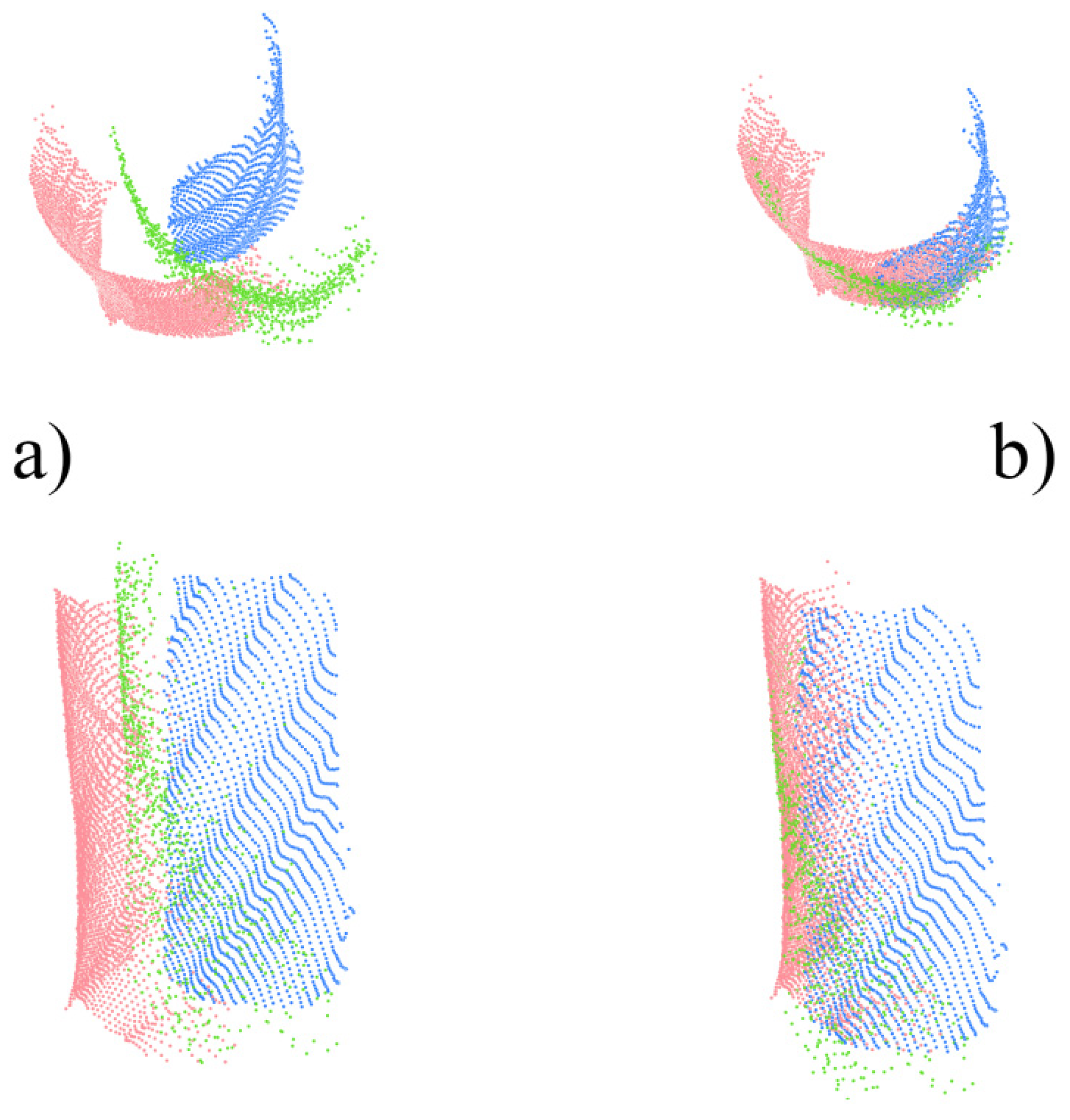
Transformed point clusters were aligned to the reference point cluster using the transformation matrix (Figure 7).
If the registration was unsuccessful, the change of several parameters was requested by the script. In most cases, only the search radius used for plane fitting (step VI) and the number of iterations were adjusted. Additionally, changes in maximum angle deviations between the normals of focal neighborhoods (with size defined by search radius) of corresponding points, maximum roughness of fitted planes, and percentage of points used for normal space sampling were also requested by the script.
Point clusters aligned in the first execution of the module were merged into one file. The horizontal overlap of merged point clusters and remaining point clusters from the same stem was calculated. If any other point cluster exhibited sufficient overlapping with merged clusters, it was aligned to them. This verification was carried out until all sufficiently overlapping point clusters were aligned (Figure 8).
Aligned point clusters were merged into one slice of the point cloud. From the slice, only point clouds with normalized height ranging from 1.275 m to 1.325 m were extracted in OPALS (Section 2.5.3).
2.5.6. Estimation of Diameter at Breast Height
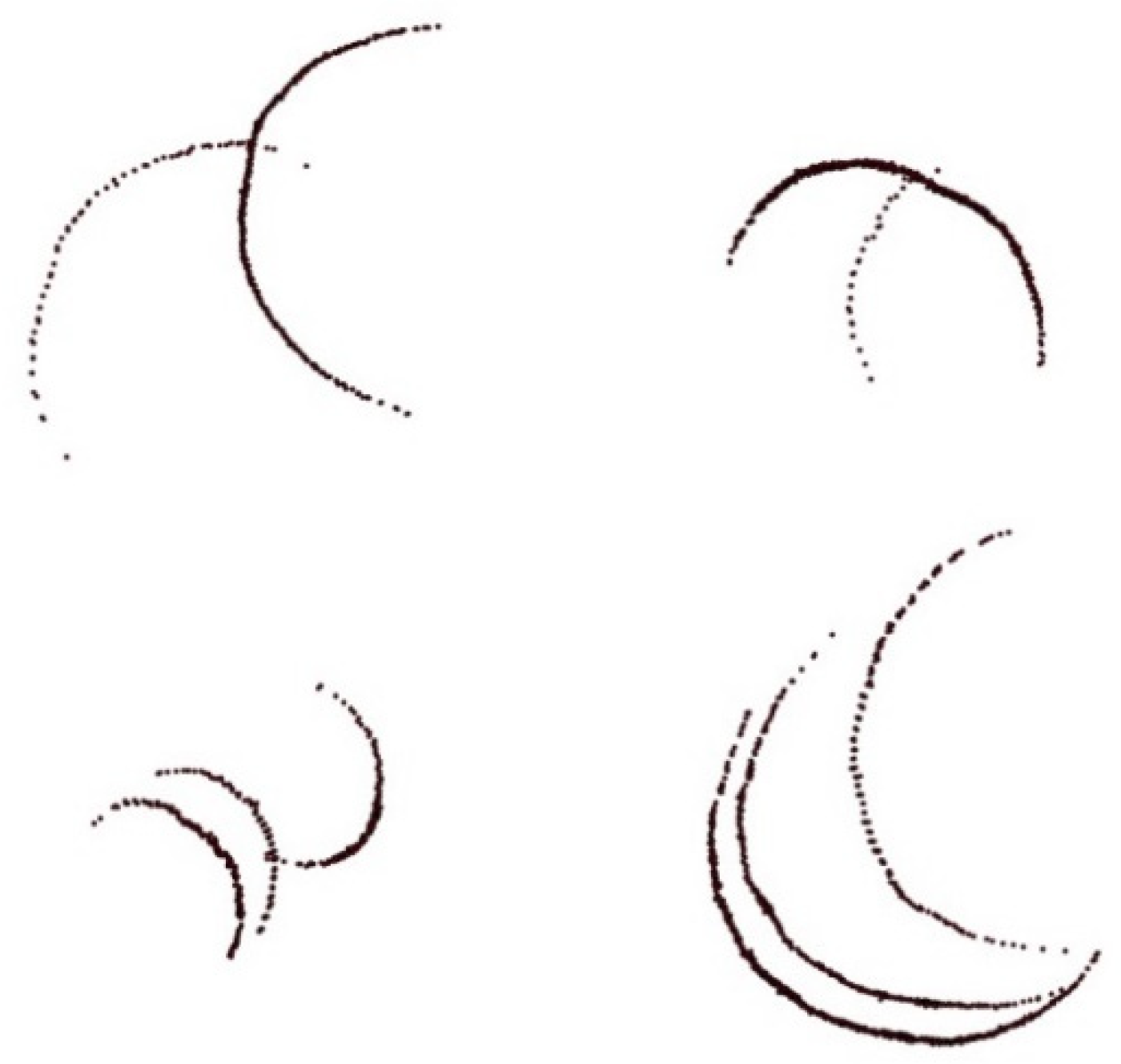
The horizontal slice of the point cloud with normalized height ranging from 1.275 m to 1.325 m was imported into the DendroCloud software [28]. Individual stems were detected using the Group by distance method. Points were clustered using 6 cm distance and only clusters with 30 points or more were considered as a tree stem.
For each detected tree stem, the diameter was estimated using the Monte Carlo method [28]. The best fitted circle was found using randomly generated circle centers and radiuses (Figure 9). The root-mean-square error of the DBH estimation is calculated as
where r is the radius of the estimated circle, and ri is the Euclidian distance between the point of the cluster and the center of the circle.
Centers and radiuses were generated until the RMSE reached values lower than 1 mm, or the number of iterations reached 2000. Estimated diameters were saved as point features with their position at the center of the estimated circle.
The estimation of DBH was tested for bias. The t-test was applied to this end. First, the error of estimation was calculated as
where d is the value of DBH estimated from MLS point cloud and D is the reference value of DBH measured using caliper during the field work.
The mean of calculated errors was then compared to 0 at 95% confidence using the t-test. Testing was performed in STATISTICA 10 software.
The bias in DBH estimation was presented in the form of a mean error. The mean error was calculated as
where is the error calculated using Equation (7) and n is the number of observations.
The accuracy of DBH estimates is presented in the form of a root-mean-square error (RMSE). The root-mean-square error was calculated as
where is the error calculated with Equation (9) and n is the number of observations.
where is the root-mean-square error obtained from Equation (9) and is mean reference diameter.
2.5.7. Estimation of MLS Coverage of Tree Stems
MLS coverage was presented in multiple studies by different names [11,14,36,37]. Bauwens et al. [14] classified the quality of the tree stem cross-section using scanning completeness of the tree, which describes the degree of ring closure for the tree stem cross-section. Pierzchala et al. [11] adapted the term support ratio, introduced by Thies and Spiecker [36] for TLS. In this paper, we adapted the term MLS coverage introduced for TLS data by Wang et al. [37]. The MLS coverage represents the percentage of a stem cross-section that is covered by the TLS point cloud [37].
Generally, MLS coverage describes the feasibility of the point cloud for the tree modeling. In order to estimate the coverage, previously created segments of points from aligned point clusters and estimated diameters in the form of point features were imported into ArcGIS 10.2. For each point cluster, the convex hull was constructed using the minimum bounding geometry tool. The convex hull was converted into a polyline feature. The polyline was edited so that only the part that is covered by points from the tree stem remained (Figure 10). Finally, the length of the edited polyline li was calculated.
For each point cluster, the circumference Ci was calculated using the value of diameter estimated by Monte Carlo method (π × d). The MLS coverage of tree stem was calculated as
3. Results
The georeferenced point cloud was divided into multiple files with similar sizes using the GNSS-IMU-based trajectory. The exported point clouds were separated corresponding to individual scanners. Pre-processed point clouds acquired using scanner 1 consisted of 242,244,607 points. Pre-processed point clouds acquired using scanner 2 consisted of 252,013,431 points. The two point clouds were then divided into 60 smaller point clouds (30 for each scanner) using boundaries of designated tiles shown in Figure 1.
3.1. GNSS Time-Based Clustering
Sixty point clouds were processed using GNSS time based the point clustering algorithm. All of the point clouds contained misaligned sets of ground points scanned from different views (Figure 11). After processing by the GNSS time-based point clustering algorithm, 58 out of 60 point clouds no longer contained any misaligned sets of ground points (Figure 12).
3.2. Matching and Registration of Point Clusters from Individual Tree Stems
Point clusters from all tree stems were compared and labeled based on their correspondence to a particular tree stem. Overall, 2153 comparisons of the point clusters were performed to match the point clusters from the same tree stems. The comparison results were investigated for a sample of 779 pairs of point clusters. Point clusters were visually examined and manually measured in LASview [34]. In addition to this, manual registration for the matched groups of point clusters was done in ArcScene 10.2. Matching of point clusters, calculation of overlap, and registration of point clusters were evaluated on the basis of omission errors, commission errors, and overall accuracy (Table 4).
With regard to the matching of point clusters, the commission error depicts an incorrect matching of a pair of point clusters from two different tree stems. The omission error represents omission of a matching point cluster pair from the same stem. The overall accuracy of point cluster matching is the percentage of correct matching from the same tree stems or omission of matching of point clusters from different tree stems. The investigation of the comparisons shows that usage of id improved overall accuracy of point clusters matching from 80.49% to 86.52%. The commission errors of the matching using only distance and id occur when the distance between the centroids of point clusters scanned from different views with erroneous positions is shorter than 1.5 m. This was mostly the case when thin stems were located near thicker stems, or another thin stem. Therefore, we added diameter differences (∆dAB) as another parameter for the matching of point clusters. The overall accuracy decreased slightly (84.72%), also while using ∆dAB for comparison of the clusters, however, the percentage of commission errors was reduced from 12.2% to 3.08% (Table 3). This is highly beneficial for following registration of the point clusters, because the commission error of matching can cause termination of ICP module or incorrect registration for point clusters from the same stem mixed with the point cluster from different tree stem. The utilization of diameter differences ∆d for the matching of point clusters caused an increase in the omission error from 1.28% to 12.2%. On the other hand, omitted point clusters in most cases cover only a small part of the tree stem, and aligning them to the rest of the point clusters does not increase the overall MLS coverage of the stem.
The horizontal overlap was calculated for matched point clusters. The commission error of the overlap calculation occurred when point clusters did not overlap to sufficient degree, and their registration was allowed. The omission error occurred when point clusters overlapped sufficiently, and in this case their registration was not allowed by the script. The overall accuracy of overlap calculation for point clusters is a percentage of correctly allowed registrations of sufficiently overlapping point clusters or correctly denied registrations of insufficiently overlapping point clusters. Overlap was checked in ArcMap 10.2 by manually finding a position of the point cluster and dividing the clusters into four zones, as it was done in the automatic calculation. In this case, the difference angle was calculated by creating a line using the direction tool in the ArcMap editor. The accuracy was 96.8%. Commission errors were observed for 0.56% of the calculations, and omission errors were observed for 2.64% of the calculations.
The registration of sufficiently overlapping point clusters was also evaluated. The overall accuracy of point cluster registration is representative of the percentage of pairs of aligned point clusters with no visible misalignment. In the case of registration, all errors were considered as commission. The overall accuracy of registration was 94.65%. Misalignment between the reference and the transformed point clusters defined as standard deviation of the residual point-to-plane distances was reported by the ICP module. The average misalignment for all aligned groups of point clusters from individual tree stems was 7.2 mm.
3.3. Estimation of Diameter at Breast Height
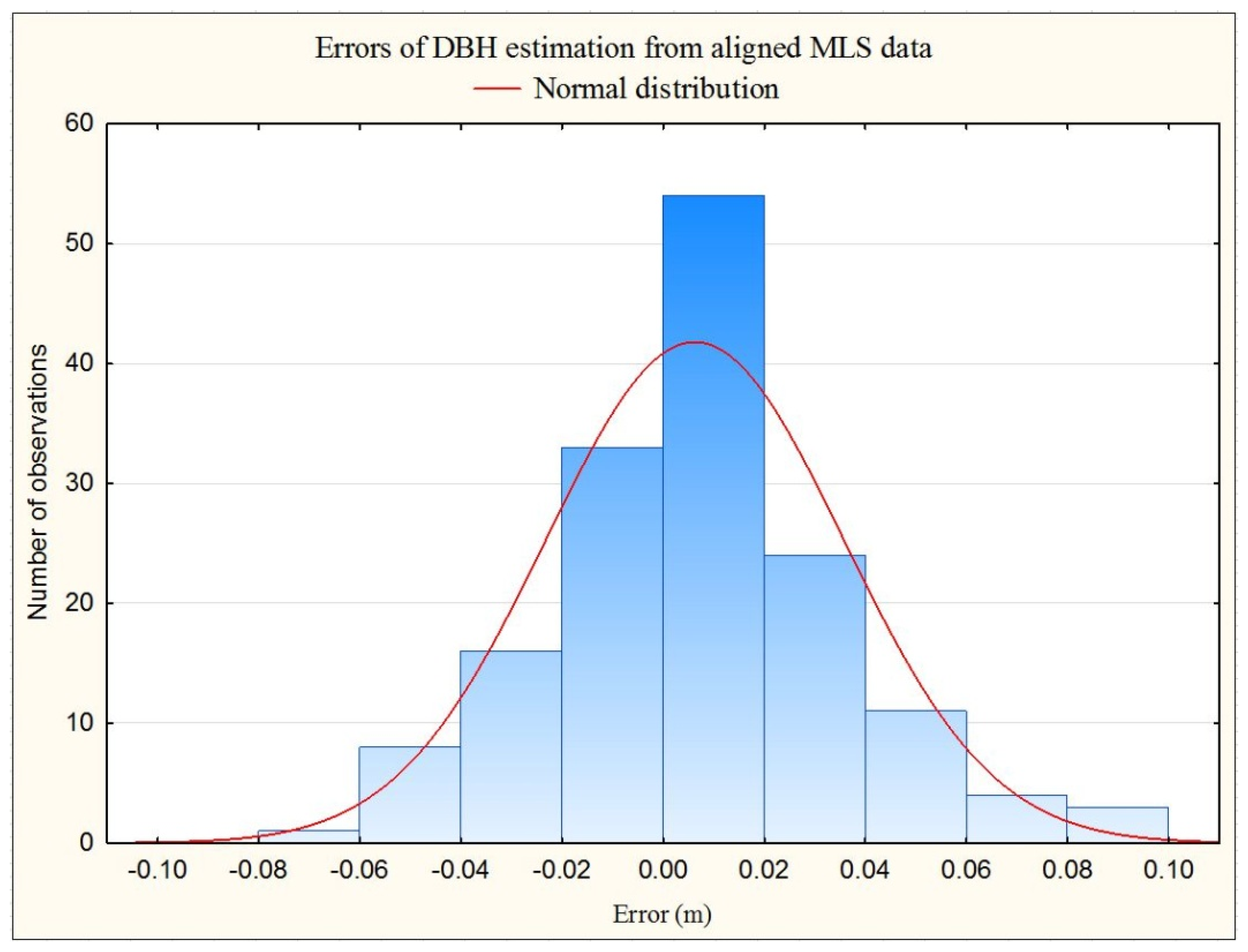
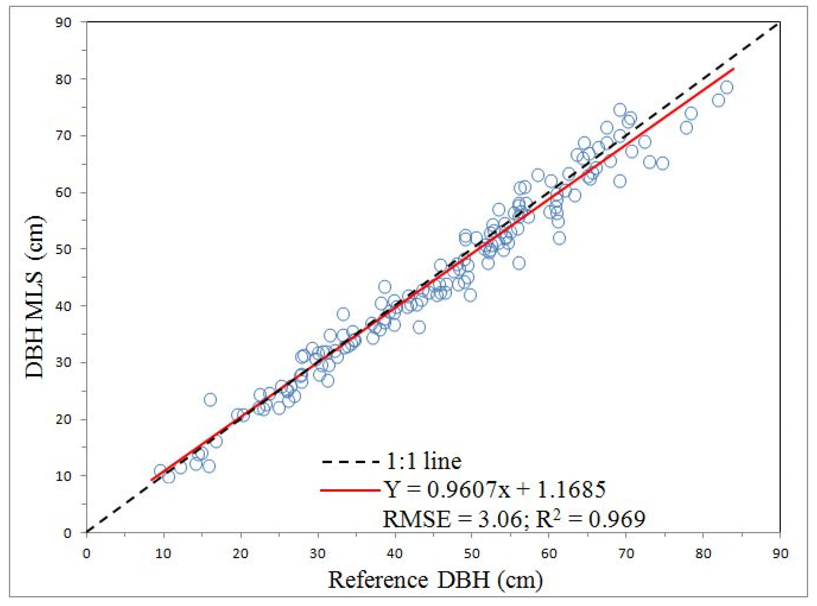
Aligned clusters from individual tree stems were merged into one-point cloud. Points of the point cloud with normalized height ranging from 1.275 m to 1.325 m were extracted and used for DBH estimation. Tree stems were detected using Group by distance method [28]. For every detected tree stem, DBH was estimated by the Monte Carlo method [28]. In some cases, tree stems were still represented by more than one point cluster, as shown in Figure 16. In these cases, only the DBH value estimated from the point cluster with the highest MLS coverage of the tree stem was chosen. The diameter was estimated for 154 tree stems and the estimated DBH values were compared with the values measured by caliper in the field. The t-test revealed the bias of DBH estimation at 95% confidence. Errors in DBH estimation varied between −7.78 cm (emin) and 9.16 cm (emax) (Figure 13). The mean error of the estimation was 0.63 cm, RMSE was 3.06 cm, and relative RMSE was 6.71% (Table 4). Nevertheless, Figure 14 shows the strong relationship between DBH values measured by caliper and the DBH estimated from MLS data.
3.4. MLS Coverage of Tree Stems
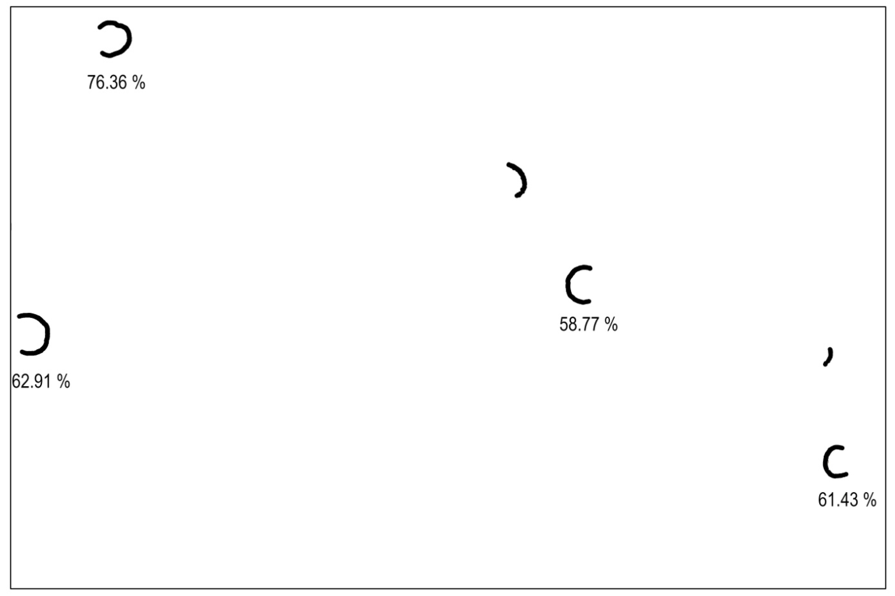
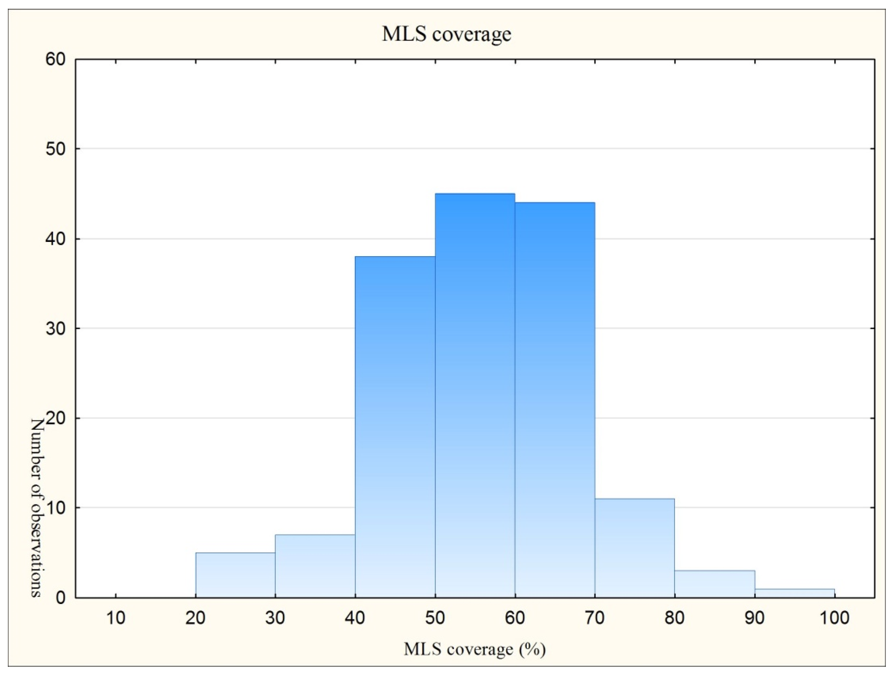
The completeness of the tree stem cross-section was evaluated using the MLS coverage parameter. In this study, the convex hull was constructed for every detected tree stem. MLS coverage of the tree stem was calculated using the circumference estimated by the Monte Carlo method and the part of the convex hull covered with points (Figure 15). MLS coverage of the tree stems ranged from 24.98% to 94% with a mean of 55.95% (Figure 16).
The relationship between the MLS coverage and the error in DBH estimation from the filtered MLS point cloud scanned from one view was shown in Čerňava et al. [20]. This relationship was also exposed for the SLAM-optimized MLS point cloud in Pierzchala et al. [11]. In the case of MLS data aligned by ICP, this relationship is not so evident, but nevertheless similar to the trend shown in Čerňava et al. [20] or Pierzchala et al. [11]. With the exception of MLS data with very low MLS coverage, the errors in DBH estimation from data with low MLS coverage shows an overestimation of the DBH values in MLS data up to 60–70% coverage. In turn, diameters estimated from MLS data with coverages higher than 70% are underestimated (Table 5).
In a previous study [20], the MLS data acquired from only one view and one VQ-250 scanner was used for DBH estimation. The RMSE of the estimation was 2.88 cm using the Monte Carlo method. However, in Čerňava et al. [20], a lot of the MLS data were filtered out. At the study site with an area of 2.93 ha, the MLS data from only 71 trees proved suitable for DBH estimation. The difference in the number of trees used for DBH estimation implies the significant improvement in the tree detection rate using the processing chain presented in this study. Furthermore, the ICP-based registration of MLS data scanned did not cause a significant increase of the RMSE of DBH estimation. In the MLS data presented in this study, the mean MLS coverage of tree stems increased from 47% to 55.95%, and the maximal MLS coverage increased from 60.6% to 94%.
4. Discussion
This study introduced the processing chain for estimation of the tree diameter from MLS data acquired under heavy forest canopy. The aim of the study was primarily to introduce a specific approach to the processing of MLS data acquired with weak GNSS signals, rather than to demonstrate the highest possible accuracy of tree diameter estimation. The MLS point cloud investigated in this study was acquired from a 110-year-old forest stand. The mean difference between two DBH values measured perpendicularly across the field, was 2.44 cm. Moreover, the maximum difference was 9 cm. This value can have a significant influence on the error of the diameter estimates from point clouds with a heterogeneously distributed point density and lower coverage of tree stems (∼50%). Better estimates of the tree diameter are expected for younger trees with more symmetric tree stems, and for point clouds with a higher coverage of tree stems.
In some MLS studies from forested areas with weak GNSS signal, the visible misalignment between the data from different views was not considered, or data scanned from distant parts of the MMS trajectory were filtered out [7,20]. This study demonstrated that the histogram of GNSS time data can be used for extraction of misaligned scenes of forest acquired using GNSS-IMU-based MLS under a heavy forest canopy. Two point clouds still contained misaligned sets of ground points even after processing the clouds using 0.001 wide histogram classes. Using smaller bin-width does not have any effect on the processing, because the GNSS time of points was recorded with 0.001 s precision. The results of GNSS time-based clustering are shown in Figure 17. As mentioned above, the division of the MLS point cloud using boundaries of the tiles shown in Figure 1 was intended for the reduction of the processing time of very dense point cloud. After processing of the MLS data, we observed that the spatial division of the data also led to discontinuity in the GNSS time data. Therefore, the data scanned from different views were separated in the histogram of GNSS time by the gaps in the histogram (bins with no observations). The gaps in the histogram of GNSS time represent time periods during which the laser beam emitted from the mobile laser scanner is occluded by the trees outside the area represented by the tile of interest, and thus the beam does not reach the trees or ground located within the tile area.
The results of our study show that the iterative closest point (ICP) algorithm can be used for aligning MLS data when GNSS outages become too long. The success of registration for sufficiently overlapping point clusters was 93.59%. The average misalignment of point clusters acquired from different views was 7.2 mm. Better alignment of the point clusters can be obtained by simply mapping the forest with a higher coverage of tree stems across the area of interest. Internal inconsistencies of tree stem locations ranging from 5 mm to 8 mm were reported by Kukko et al. [10] using Graph-SLAM-optimized MLS data.
One of the flaws of the introduced processing chain is semi-automatic tree detection. While the tree stem can be detected using the group by distance method [28], some non-tree objects can be also classified as a tree and have to be manually removed from the point cloud. Furthermore, the point clouds from tree stems detected by group by distance method can contain some point noise, which was also filtered manually in this study. The manual filtration was done due to relatively low occurrence of noise, but can be substituted by point-density-based filtering methods contained in presented software [29,30,31,34]. More efficient detection of tree stems can be also achieved by using cylinder-fitting methods such as that of Liang et al. [38]. Proposed processing chain also utilizes multiple software products. The used software products are originally developed for processing of ALS data with lower point density. Although the OPALS software offer the tools for ground points classification, in order to obtain set of ground with resolution and accuracy similar to the presented processing chain, combination of multiple tools is required.
In this study, the RMSE of DBH estimation was 3.06 cm using the ICP-based processing chain developed for estimation of the tree diameter from TLS data [28]. The presented DBH estimation is also biased. A correction of the bias could potentially increase the accuracy of DBH estimation. This result is similar to accuracy of Monte Carlo based DBH estimation from single scan TLS data and lower comparing to multi-scan data [28]. Authors of MLS studies report also similar [7] or even lower accuracy [15,38]. Study of Wu et al. [19] showed that higher accuracy of DBH estimation from MLS can be achieved in urban forests. Higher accuracy was also reported by Ryding et al. [12], Bauwens et al. [14] and Cabo et al. [16] for DBH estimated from HMLS, using cylinder fitting. Pierzchala et al. [11] achieved slightly higher accuracy of DBH estimation from the point cloud generated using Graph-SLAM from the ICP-based laser odometry.
It is important to mention that the mean MLS coverage of the tree stems was 55.95% in this study, even after the alignment of point cloud slices scanned from different views. Table 5 shows that the DBH estimation from MLS data with coverages above 60% are more accurate (RMSE = 2.05–2.19 cm). The coverage obtained is much lower compared to e.g., Bauwens et al. [14] with MLS coverages of 100% for 91% of the tree stems (RMSEDBH = 1.11 cm). The MLS coverage in this study is more similar to the results of Pierzchala et al. [11] (RMSEDBH = 2.38 cm). This comparison shows that MLS coverage has a significant influence on the accuracy of DBH estimation, and therefore much more attention should be paid to the selection of a more adaptable platform for MLS and the selection of mapping trajectories in future studies.
5. Conclusions
We have developed a processing chain for the extraction of forest scenes scanned from different views from misaligned MLS point clouds, and consequent registration of the scenes using ICP. This study demonstrates that GNSS time data can be used both to separate the scenes of forest stands scanned at different time periods from the spatially extracted point cloud, and to match the MLS data from individual trees. The point clouds obtained from the forest stand with continuous time data can be divided using gaps in the histogram of the time data after being spatially tiled or divided using polygon geometry, as it was shown in the study. This processing can result in the extraction of point clouds without vertically shifting the forest scenes even without sufficient GNSS signal. However, GNSS time-based clustering used in the study caused loss of 33.48% of the points for both point clouds from the two Riegl VMX-250 scanners. The matching of point clusters from individual tree stems was successful for 84.72% of the compared pairs of point clusters. The level of automation for the registration of point clusters from the stems was improved using the method for calculation of horizontal overlap of the clusters in 96.8% of the cases. Registration was successful in 94.65% of the cases using the ICP algorithm in the OPALS system. An average misalignment of 7.2 mm was observed for the aligned point clusters.
The DBH was estimated from aligned MLS point clouds for 154 trees. The RMSE of the estimation was 3.06 cm. This accuracy is comparable with GNSS-IMU-based MLS studies, but is lower compared to the majority of SLAM-based MLS studies. Results also show that the accuracy of DBH estimation differs based on the MLS coverage of the tree stems. Therefore, higher accuracy can be expected for MLS data with high MLS coverage (RMSE = 2.05–2.19 cm for MLS data with coverage of tree stems above 60%). The accuracy achieved in this study is likewise comparable with SLAM-based MLS studies that used MLS data with a similar coverage of tree stems. The processing chain can be improved using additional data from the GNSS-IMU system, such as dilution of precision, in order to further increase the level of automation for the processing of MLS data. Future studies should also investigate the accuracy and efficiency of tree parameter estimation from MLS data with high MLS coverages of tree stems.
Author Contributions
J.T. acquired funding for the mobile laser scanning and supervised the acquisition of mobile laser scanning data. J.Č. developed the workflow for MLS data processing. J.Č. and Z.S. processed the data in OPALS. J.Č., M.A., and J.T. acquired reference data on tree diameters. J.Č. estimated the diameters in DendroCloud and performed the statistical analyses. M.M. validated the statistical analyses and results. J.Č. proposed the original manuscript. The manuscript was checked by M.M., J.T., and M.A. and corrected by J.Č. and M.M. M.M. acquired funding for publication of the manuscript.
Funding
This work was supported by grant no. CZ.02.1.01/0.0/0.0/16_019/0000803 (“Advanced research supporting the forestry and wood-processing sector’s adaptation to global change and the 4th industrial revolution”) financed by OP RDE. The work was also supported by grants VEGA 1/0953/13 (“Geographic information on forest and forest landscape: Specifics of creation and application”) and VEGA 1/0881/17 (“Mobile geographical data collection on forest and landscape”) financed by the Scientific Grant Agency of the Ministry of Education, Science, Research and Sport of the Slovak Republic.
Conflicts of Interest
The authors declare no conflict of interest.
References
- Optech Inc. Mobile Mapping System Lynx. 2007. Available online: https://www.teledyneoptech.com (accessed on 12 March 2019).
- MDL Laser Systems 2010. Mobile Mapping System Dynascan. Available online: https://www.renishaw.com (accessed on 12 March 2019).
- RIEGL Laser Measurement Systems GmbH 2010. Mobile Mapping System Riegl VMX-250. Available online: http://www.riegl.com (accessed on 12 March 2019).
- Topcon Corporation 2010. Mobile Mapping System IP-S2. Available online: https://www.topcon.co.jp/ (accessed on 12 March 2019).
- SITECO Inf. Mobile mapping system Roadscanner. 2012. Available online: www.sitecoinf.it/it/ (accessed on 12 March 2019).
- Puente, I.; González-Jorge, H.; Martínez-Sánchez, J.; Arias, P. Review of mobile mapping and surveying technologies. Meas. J. Int. Meas. Confed. 2013, 46, 2127–2145. [Google Scholar] [CrossRef]
- Liang, X.; Hyyppa, J.; Kukko, A.; Kaartinen, H.; Jaakkola, A.; Yu, X. The use of a mobile laser scanning system for mapping large forest plots. IEEE Geosci. Remote Sens. Lett. 2014, 11, 1504–1508. [Google Scholar] [CrossRef]
- Liang, X.; Kukko, A.; Kaartinen, H.; Hyyppä, J.; Yu, X.; Jaakkola, A.; Wang, Y. Possibilities of a personal laser scanning system for forest mapping and ecosystem services. Sensors 2014, 14, 1228–1248. [Google Scholar] [CrossRef] [PubMed]
- Rönnholm, P.; Liang, X.; Kukko, A.; Jaakkola, A.; Hyyppä, J. Quality analysis and correction of mobile backpack laser scanning data. ISPRS Ann. Photogramm. Remote Sens. Spat. Inf. Sci. 2016, 3, 41–47. [Google Scholar] [CrossRef]
- Kukko, A.; Kaijaluoto, R.; Kaartinen, H.; Lehtola, V.V.; Jaakkola, A.; Hyyppä, J. Graph SLAM correction for single scanner MLS forest data under boreal forest canopy. ISPRS J. Photogramm. Remote Sens. 2017, 132, 199–209. [Google Scholar] [CrossRef]
- Pierzchała, M.; Giguère, P.; Astrup, R. Mapping forests using an unmanned ground vehicle with 3D LiDAR and graph-SLAM. Comput. Electron. Agric. 2018, 145, 217–225. [Google Scholar] [CrossRef]
- Ryding, J.; Williams, E.; Smith, M.J.; Eichhorn, M.P. Assessing handheld mobile laser scanners for forest surveys. Remote Sens. 2015, 7, 1095–1111. [Google Scholar] [CrossRef]
- Tang, J.; Chen, Y.; Kukko, A.; Kaartinen, H.; Jaakkola, A.; Khoramshahi, E.; Hakala, T.; Hyyppä, J.; Holopainen, M.; Hyyppä, H. SLAM-aided stem mapping for forest inventory with small-footprint mobile LiDAR. Forests 2015, 6, 4588–4606. [Google Scholar] [CrossRef]
- Bauwens, S.; Bartholomeus, H.; Calders, K.; Lejeune, P. Forest inventory with terrestrial LiDAR: A comparison of static and hand-held mobile laser scanning. Forests 2016, 7, 127. [Google Scholar] [CrossRef]
- Forsman, M.; Holmgren, J.; Olofsson, K. Tree stem diameter estimation from mobile laser scanning using line-wise intensity-based clustering. Forests 2016, 7, 206. [Google Scholar] [CrossRef]
- Cabo, C.; Del Pozo, S.; Rodríguez-Gonzálvez, P.; Ordóñez, C.; González-Aguilera, D. Comparing terrestrial laser scanning (TLS) and wearable laser scanning (WLS) for individual tree modeling at plot level. Remote Sens. 2018, 10, 540. [Google Scholar] [CrossRef]
- Puttonen, E.; Jaakkola, A.; Litkey, P.; Hyyppä, J. Tree classification with fused mobile laser scanning and hyperspectral data. Sensors 2011, 11, 5158–5182. [Google Scholar] [CrossRef]
- Holopainen, M.; Kankare, V.; Vastaranta, M.; Liang, X.; Lin, Y.; Vaaja, M.; Yu, X.; Hyyppä, J.; Hyyppä, H.; Kaartinen, H. Tree mapping using airborne, terrestrial and mobile laser scanning–A case study in a heterogeneous urban forest. Urban For. Urban Green. 2013, 12, 546–553. [Google Scholar] [CrossRef]
- Wu, B.; Yu, B.; Yue, W.; Shu, S.; Tan, W.; Hu, C.; Huang, Y.; Wu, J.; Liu, H. A voxel-based method for automated identification and morphological parameters estimation of individual street trees from mobile laser scanning data. Remote Sens. 2013, 5, 584–611. [Google Scholar] [CrossRef]
- Čerňava, J.; Tuček, J.; Koreň, M.; Mokroš, M. Estimation of diameter at breast height from mobile laser scanning data collected under a heavy forest canopy. J. For. Sci. 2017, 63, 433–441. [Google Scholar] [CrossRef] [Green Version]
- Chen, Y.; Medioni, G. Object modelling by registration of multiple range images. Image Vis. Comput. 1992, 10, 145–155. [Google Scholar] [CrossRef]
- Besl, P.J.; McKay, N.D. A Method for Registration of 3-D Shapes. Trans. Pattern Anal. Mach. Intell. 1991, 14, 239–256. [Google Scholar] [CrossRef]
- MathWorks, M. SIMULINK for Technical Computing. 2015. Available online: https://www.mathworks.com/ (accessed on 12 March 2019).
- CloudCompare. GPL Software.; (version 2.6.2). Available online: http://www.cloudcompare.org/ (accessed on 12 March 2019).
- Glira, P.; Pfeifer, N.; Briese, C.; Ressl, C. A Correspondence Framework for ALS Strip Adjustments based on Variants of the ICP Algorithm. Photogramm. Fernerkundung Geoinf. 2015, 2015, 275–289. [Google Scholar] [CrossRef]
- Glira, P.; Pfeifer, N.; Mandlburger, G. Rigorous Strip adjustment of UAV-based laserscanning data including time-dependent correction of trajectory errors. Photogramm. Eng. Remote Sens. 2016, 82, 945–954. [Google Scholar] [CrossRef]
- Liang, X.; Kukko, A.; Hyyppä, J.; Lehtomäki, M.; Pyörälä, J.; Yu, X.; Kaartinen, H.; Jaakkola, A.; Wang, Y. In-situ measurements from mobile platforms: An emerging approach to address the old challenges associated with forest inventories. ISPRS J. Photogramm. Remote Sens. 2018, 143, 97–107. [Google Scholar] [CrossRef]
- Koreň, M.; Mokroš, M.; Bucha, T. Accuracy of tree diameter estimation from terrestrial laser scanning by circle-fitting methods. Int. J. Appl. Earth Obs. Geoinf. 2017, 63, 122–128. [Google Scholar] [CrossRef]
- Mandlburger, G.; Otepka, J.; Karel, W.; Wagner, W.; Pfeifer, N. Orientation and processing of airborne laser scanning data (OPALS)—Concept and first results of a comprehensive ALS software. IAPRS 2009, XXXVIII, 55–60. [Google Scholar]
- Otepka, J.; Mandlburger, G.; Karel, W. The OPALS data manager—Efficient data management for processing large airborne laser scanning projects. ISPRS Ann. Photogramm. Remote Sens. Spat. Inf. Sci. 2012, 1, 153–159. [Google Scholar] [CrossRef]
- Pfeifer, N.; Mandlburger, G.; Otepka, J.; Karel, W. OPALS—A framework for Airborne Laser Scanning data analysis. Comput. Environ. Urban Syst. 2014, 45, 125–136. [Google Scholar] [CrossRef]
- Simanov, V.; Macků, J.; Popelka, J. Proposal of a new terrain classification and technological typification. Lesnictví 1993, 39, 422–428. [Google Scholar]
- Boavida, J.; Oliveira, A.; Santos, B. Precise long tunnel survey using the Riegl VMX-250 mobile laser scanning system. In Proceedings of the 2012 RIEGL International Airborne and Mobile User Conference, Orlando, FL, USA, 27 February–1 March 2012; Volume 27. [Google Scholar]
- Isenburg, M. LAStools—Efficient LiDAR Processing Software, (version 160429, Academic); rapidlasso GmbH: Gilching, Germany, 2016. [Google Scholar]
- Rusinkiewicz, S.; Levoy, M. Efficient variants of the ICP algorithm. In Proceedings of the Third International Conference on 3-D Digital Imaging and Modeling, Quebec City, QC, Canada, 28 May–1 June 2001; pp. 145–152. [Google Scholar]
- Thies, M.; Spiecker, H.; Str, T. Evaluation and future prospects of terrestrial laser scanning for standardized laser scanning for standardized forest inventories. Int. Arch. Photogramm. Remote Sens. 2004, 36, 192–197. [Google Scholar]
- Wang, D.; Hollaus, M.; Puttonen, E.; Pfeifer, N. Automatic and Self-Adaptive Stem Reconstruction in Landslide-Affected Forests. Remote Sens. 2016, 8, 974. [Google Scholar] [CrossRef]
- Liang, X.; Litkey, P.; Hyyppa, J.; Kaartinen, H.; Vastaranta, M.; Holopainen, M. Automatic stem mapping using single-scan terrestrial laser scanning. IEEE Trans. Geosci. Remote Sens. 2012, 50, 661–670. [Google Scholar] [CrossRef]
Figure 1.
Location of study site within the borders of the Slovak Republic is shown in the upper part of the figure. The study area divided into irregular tiles, tree locations, and the trajectory of the MMS are shown in the lower part of the figure. Tree locations were estimated from the fully processed MLS point cloud.

Figure 2.
Mobile mapping system RIEGL VMX-250 mounted on tractor Zetor Horal 7245. Two digital cameras (1) and mobile laser scanners VQ-250 (2) are placed on the side of the MMS measuring head. The GNSS antenna (3) is placed on the top of the measuring head and the panoramic camera (4) is placed above the MMS measuring head (Source: Čerňava et al. [20]).

Figure 3.
Intersecting point clusters reflected from four tree stems. The spatial relationship between these groups of point clusters was modified for a better demonstration of misalignment.
Figure 3.
Intersecting point clusters reflected from four tree stems. The spatial relationship between these groups of point clusters was modified for a better demonstration of misalignment.

Figure 4.
Principle of GNSS time based point clustering. Centers of histogram gaps, which were used for dividing the point cloud, are highlighted by red lines.
Figure 4.
Principle of GNSS time based point clustering. Centers of histogram gaps, which were used for dividing the point cloud, are highlighted by red lines.

Figure 5.
Estimation of point cluster diameter. Estimated diameters are shown above the point clusters. Circle estimated using maximal distance (a). Circle estimated using circle-fitting method and generalized geometry of point cluster (b). Optimization of the circle fit using all points of the cluster (c).

Figure 6.
Calculation of direction angles for two point clusters of interest. Calculation of direction angle (a). Calculation of the direction angle and angle range in point cluster with points containing direction angles ranging from 360 - ga° to 360° (b). Direction angles range from 76.02° to 239.68° for point clusters shown in (a). For the point cluster shown in (b), the angles range from 311.49° to 169.03°. The horizontal overlap of the point clusters is 93.02°.

Figure 7.
Point clusters from the same tree stem before (a) and after the registration (b).

Figure 8.
The workflow of registration of point clusters from individual tree stems.

Figure 9.
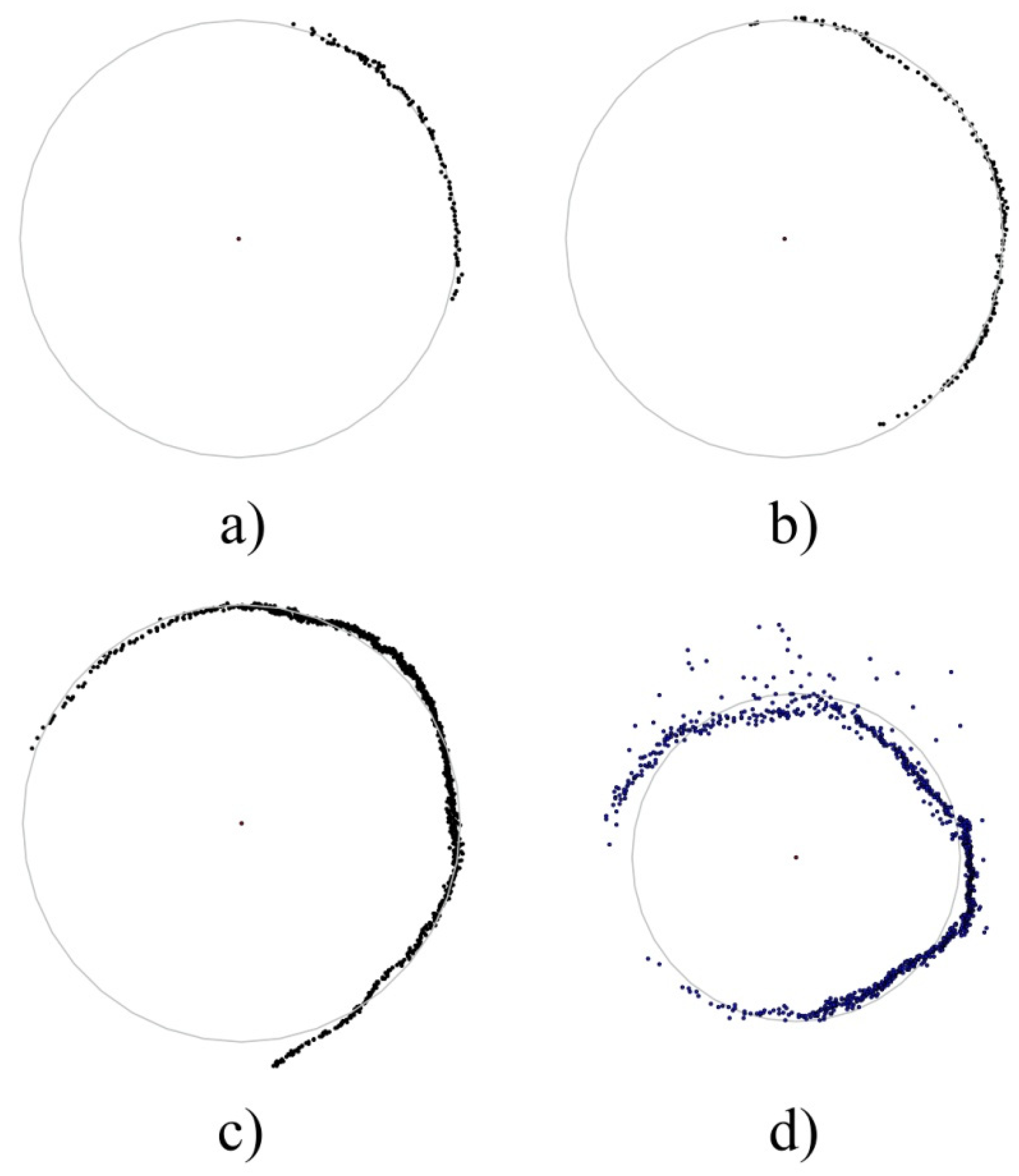
Diameter estimation by the Monte Carlo method. Percentage MLS coverage for (a) 25.85% for (b), 45.28%, for (c) 68.84%, and for (d) 94%. Point clusters (c,d) consist of multiple point clusters each, scanned from different views and aligned by the ICP algorithm introduced by Glira et al. [35].
Figure 9.
Diameter estimation by the Monte Carlo method. Percentage MLS coverage for (a) 25.85% for (b), 45.28%, for (c) 68.84%, and for (d) 94%. Point clusters (c,d) consist of multiple point clusters each, scanned from different views and aligned by the ICP algorithm introduced by Glira et al. [35].

Figure 10.
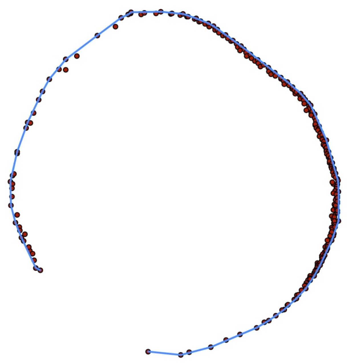
Edited convex hull representing MLS coverage of a tree stem. The point cluster portrayed in the figure consists of multiple point clusters obtained from different views and aligned by the ICP algorithm introduced in Glira et al. [25].
Figure 10.
Edited convex hull representing MLS coverage of a tree stem. The point cluster portrayed in the figure consists of multiple point clusters obtained from different views and aligned by the ICP algorithm introduced in Glira et al. [25].

Figure 11.
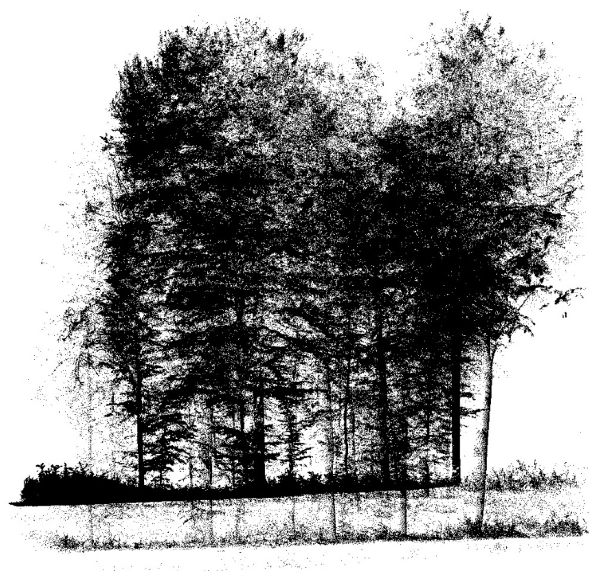
Part of the pre-processed point cloud extracted using the geometry of one of the polygons shown in Figure 1.
Figure 11.
Part of the pre-processed point cloud extracted using the geometry of one of the polygons shown in Figure 1.

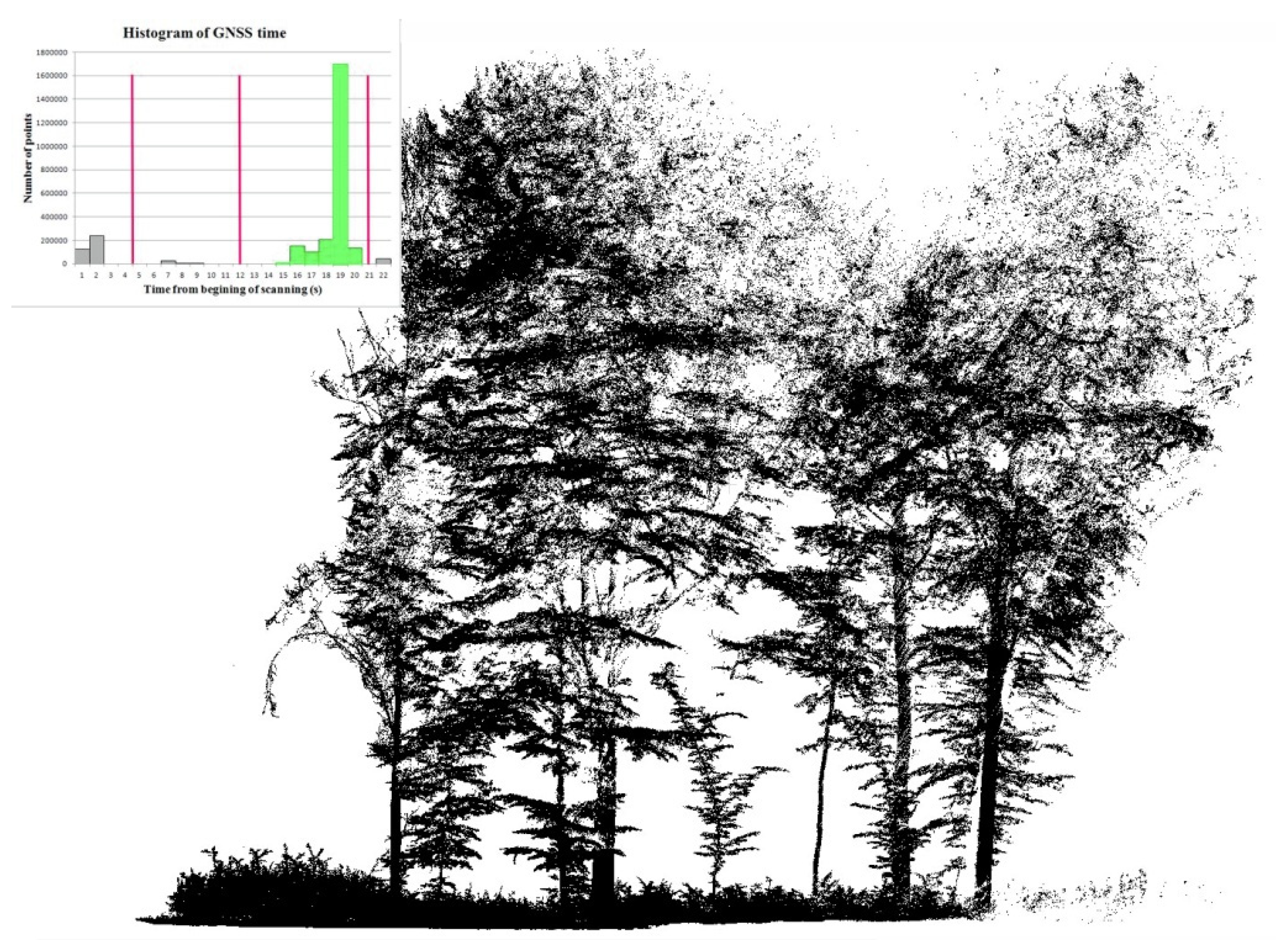
Figure 12.
One of the point clouds extracted from the point cloud shown in Figure 11 using GNSS time-based point clustering. The point cloud consists of the highest number of points. The histogram of GNSS time for the point cloud is shown in the upper left part of the figure. The part of the histogram that corresponds to the displayed point cloud is highlighted in green.

Figure 13.
Histogram of errors in DBH estimation from the aligned MLS point cloud.

Figure 14.
Scatterplot of DBH estimations from MLS and reference DBH measured by caliper.

Figure 15.
Horizontal slice of the processed point cloud. Values of MLS coverage of tree stem are depicted under the point clusters of tree stems.
Figure 15.
Horizontal slice of the processed point cloud. Values of MLS coverage of tree stem are depicted under the point clusters of tree stems.

Figure 16.
Histogram of MLS coverage values.

Figure 17.
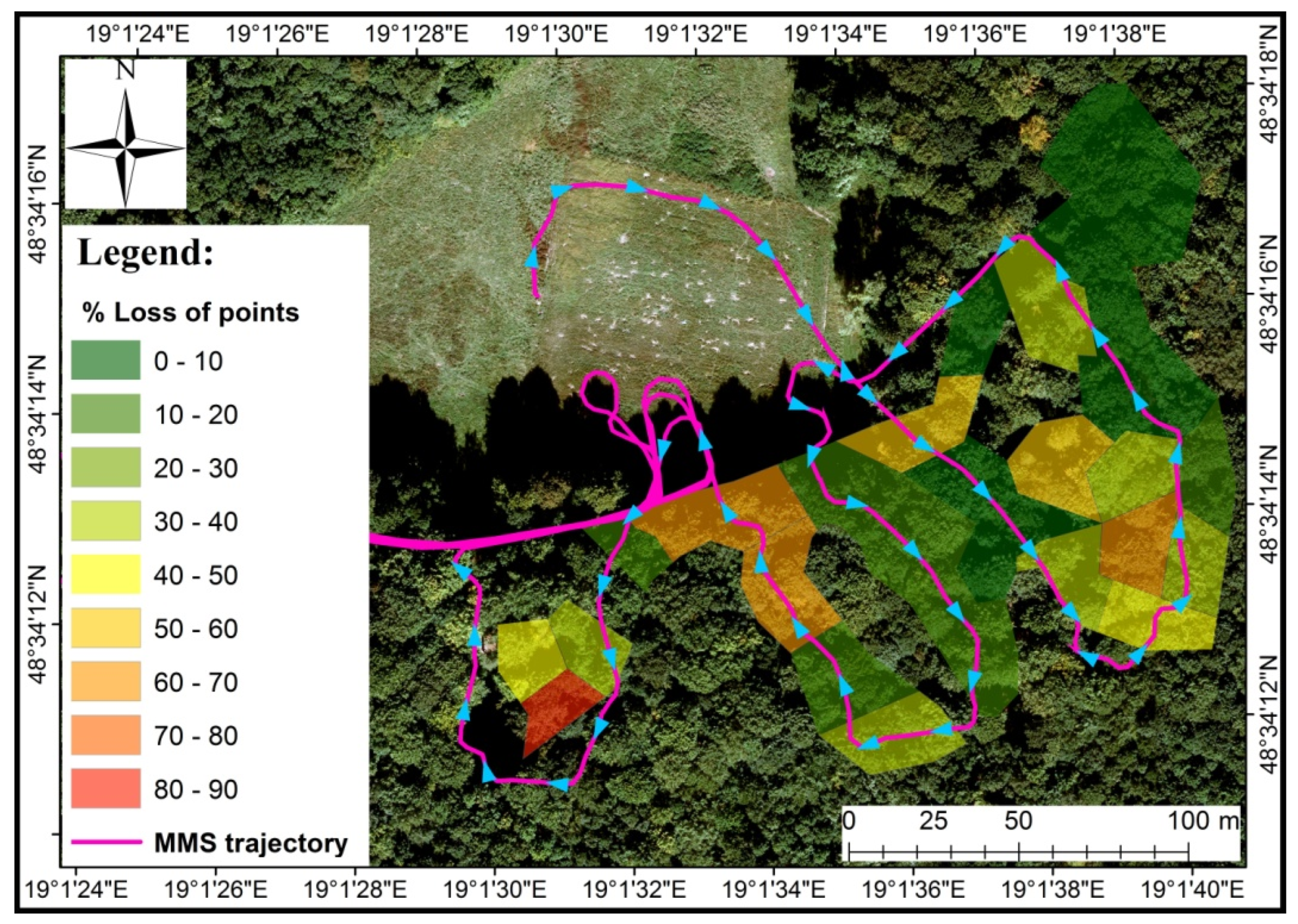
Percentage loss of points after GNSS time-based clustering for individual tiles located within the study site. The direction of the MMS trajectory is highlighted by teal arrows.
Figure 17.
Percentage loss of points after GNSS time-based clustering for individual tiles located within the study site. The direction of the MMS trajectory is highlighted by teal arrows.


Table 1.
Mobile mapping system physical data
| MMS Physical Data | Main Dimension (L × W × H) (mm) | Weight (kg) |
|---|---|---|
| VMX-250-MH Measuring head | 737 × 456 × 485 | 43 |
| VMX-250-CU Control Unit | 560 × 455 × 265 | 26 |
| VMX-250-CS6 Camera System | 607 × 1038 × 208 | 19 |
Table 2.
Technical specification of IMU/GNSS and the mobile laser scanner
| GNSS-IMU Performance | |
| Parameter | Value |
| Position (absolute) (mm) | 20–50 |
| Position (relative) (mm) | 10 |
| Roll and Pitch (°) | 0.005 |
| Heading (°) | 0.015 |
| Mobile Laser Scanner VQ-250 | |
| Parameter | Value |
| Laser Measuring Principle | Time of flight |
| Horizontal Field of View (°) | 360 |
| Vertical Field of View (°) | 360 |
| Minimum Measurement Range (m) | 1.5 |
| Maximum Measurement Range (m) | 200 |
| Accuracy (mm) | 10 |
| Precision (mm) | 5 |
| Laser Pulse Repetition Rate (kHz) | 300 |
| Max. Effective Measurement Rate (pnts/s) | 300000 |
| Laser Wavelength | Near-infrared |
| Laser Beam Divergence (mrad) | 0.35 |
| Laser Beam Footprint (mm/50 m) | 18 |
| Angle Measurement Resolution (°) | 0.001 |
Table 3.
Results of matching and registration of point clusters. Separated accuracies and errors are reported for matching using only distance between the centroids of the compared point clusters (dist.), matching using the distance and index of duplicity (dist. + id) and matching using the distance, index of duplicity and difference between the diameters of the compared point clusters (dist. + id + ∆d).
| Processing Step | Matching | Overlap Calculation | Registration | ||||
|---|---|---|---|---|---|---|---|
| Parameters | dist. | dist. + id | dist. + id + ∆d | ||||
| Sample size | 779 | 779 | 779 | 531 | 430 | ||
| Accuracy | Absolute | 627 | 674 | 660 | 514 | 407 | |
| Relative (%) | 80.49 | 86.52 | 84.72 | 96.8 | 94.65 | ||
| Errors | Commission | Number | 152 | 95 | 24 | 3 | 23 |
| Percentage (%) | 19.51 | 12.2 | 3.08 | 0.56 | 2.9 | ||
| Omission | Number | 0 | 10 | 95 | 14 | 0 | |
| Percentage (%) | 0 | 1.28 | 12.2 | 2.64 | 0 | ||
Table 4.
Overall results of DBH estimation for whole sample with size N and mean diameter . Minimum (emin), maximum (emax), mean error (), absolute (RMSE) and relative root-mean-square error (RMSE%) in the estimation are shown. The shown p-value was calculated from errors (Equation (7)) using t-test at 95% confidence.
| N | p-Value | emin (cm) | emax (cm) | RMSE (cm) | RMSE% (%) | ||
|---|---|---|---|---|---|---|---|
| 154 | 45.02 | 0.0091 | −7.78 | 9.16 | 0.63 | 3.06 | 6.71 |
Table 5.
Mean error (), absolute root-mean-square error (RMSE) and relative root-mean-square error (%RMSE) in DBH estimation from individual aligned MLS point clouds for different MLS coverage extent with sample size of N and mean diameter of .
Table 5.
Mean error (), absolute root-mean-square error (RMSE) and relative root-mean-square error (%RMSE) in DBH estimation from individual aligned MLS point clouds for different MLS coverage extent with sample size of N and mean diameter of .
| MLS Coverage (%) | N | RMSE (cm) | %RMSE (%) | ||
|---|---|---|---|---|---|
| 20–30 | 5 | 58.30 | −2.39 | 3.53 | 6.06 |
| 30–40 | 7 | 54.08 | 1.44 | 6.74 | 12.46 |
| 40–50 | 38 | 44.88 | 1.22 | 3.11 | 6.92 |
| 50–60 | 45 | 42.68 | 0.73 | 3.13 | 7.33 |
| 60–70 | 44 | 46.51 | 0.84 | 2.05 | 4.41 |
| 70–80 | 11 | 38.63 | −1.14 | 2.17 | 5.61 |
| 80+ | 4 | 41.31 | −1.34 | 2.19 | 5.31 |
© 2019 by the authors. Licensee MDPI, Basel, Switzerland. This article is an open access article distributed under the terms and conditions of the Creative Commons Attribution (CC BY) license (http://creativecommons.org/licenses/by/4.0/).
Share and Cite
MDPI and ACS Style
Čerňava, J.; Mokroš, M.; Tuček, J.; Antal, M.; Slatkovská, Z. Processing Chain for Estimation of Tree Diameter from GNSS-IMU-Based Mobile Laser Scanning Data. Remote Sens. 2019, 11, 615. https://0-doi-org.brum.beds.ac.uk/10.3390/rs11060615
AMA Style
Čerňava J, Mokroš M, Tuček J, Antal M, Slatkovská Z. Processing Chain for Estimation of Tree Diameter from GNSS-IMU-Based Mobile Laser Scanning Data. Remote Sensing. 2019; 11(6):615. https://0-doi-org.brum.beds.ac.uk/10.3390/rs11060615
Chicago/Turabian StyleČerňava, Juraj, Martin Mokroš, Ján Tuček, Michal Antal, and Zuzana Slatkovská. 2019. "Processing Chain for Estimation of Tree Diameter from GNSS-IMU-Based Mobile Laser Scanning Data" Remote Sensing 11, no. 6: 615. https://0-doi-org.brum.beds.ac.uk/10.3390/rs11060615
Note that from the first issue of 2016, this journal uses article numbers instead of page numbers. See further details here.