An Automated Rectification Method for Unmanned Aerial Vehicle LiDAR Point Cloud Data Based on Laser Intensity


1
Institute of Remote Sensing and Geographic Information System, Peking University, 5 Summer Palace Road, Beijing 100871, China
2
Guangdong Research Institute of Water Resources and Hydropower, Guangzhou 510635, China
*
Author to whom correspondence should be addressed.
Remote Sens. 2019, 11(7), 811; https://0-doi-org.brum.beds.ac.uk/10.3390/rs11070811
Submission received: 2 March 2019
/
Revised: 29 March 2019
/
Accepted: 1 April 2019
/
Published: 4 April 2019
(This article belongs to the Section Remote Sensing Image Processing)
Abstract
:Point cloud rectification is an efficient approach to improve the quality of laser point cloud data. Conventional rectification methods mostly relied on ground control points (GCPs), typical artificial ground objects, and raw measurements of the laser scanner which impede automation and adaptability in practice. This paper proposed an automated rectification method for the point cloud data that are acquired by an unmanned aerial vehicle LiDAR system based on laser intensity, with the goal to reduce the dependency of ancillary data and improve the automated level of the rectification process. First, laser intensity images were produced by interpolating the intensity data of all the LiDAR scanning strips. Second, a scale-invariant feature transform algorithm was conducted to extract two dimensional (2D) tie points from the intensity images; the pseudo tie points were removed by using a random sample consensus algorithm. Next, all the 2D tie points were transformed to three dimensional (3D) point cloud to derive 3D tie point sets. After that, the observation error equations were created with the condition of coplanar constraints. Finally, a nonlinear least square algorithm was applied to solve the boresight angular error parameters, which were subsequently used to correct the laser point cloud data. A case study in Shehezi, Xinjiang, China was implemented with our proposed method and the results indicate that our method is efficient to estimate the boresight angular error between the laser scanner and inertial measurement unit. After applying the results of the boresight angular error solution to rectify the laser point cloud, the planar root mean square error (RMSE) is 5.7 cm and decreased by 1.1 cm in average; the elevation RMSE is 1.4 cm and decreased by 0.8 cm in average. Comparing with the stepwise geometric method, our proposed method achieved similar horizontal accuracy and outperformed it in vertical accuracy of registration.
1. Introduction
Unmanned aerial vehicle (UAV) Light Detection and Ranging (LiDAR) is a new technology in the field of survey and mapping that is equipped with low-altitude UAV platform for LiDAR data acquisition and composed of three core components, including laser measurement, differential Global Navigation Satellite System (GNSS), and inertial navigation unit (IMU) [1,2]. Comparing with conventional aerial photogrammetry techniques, UAV LiDAR bears a number of advantages such as being less impacted by flying conditions (e.g., cloud cover and flexible ground control), high-level automation, more precision and density data, and high flexibility. Thus, it has been widely used in acquiring digital elevation model [3,4,5], disaster monitoring [6], heritage protection [7], forestry survey [8,9,10,11], and 3D modeling [12]. In these applications, attention was often given to the surveying accuracy of height or altitude, which is important for most situations. Among those factors that degrade the surveying accuracy of UAV LiDAR data [13,14,15], boresight angular error is a systematic error and has significant influence on the geolocation of laser points [15,16]. It usually happens during the payload installation of a UAV LiDAR system and the unstable UAV flying process, and consequently the boresight angular error cannot be considered to be negligible and is hard to be directly measured [17,18]. Moreover, it can lead to systematic positional deviations in all LiDAR scanning strips and misalignment of the same objects in overlapping areas in different LiDAR scanning strips [19,20]. Therefore, it is necessary to estimate and reduce down the errors in LiDAR point data processing. Obviously the accuracy of laser points has significant impact on the quality of mapping products, especially for applications such as matching and fusion of multisource remote sensing data [15,21]. Thus, it is currently a key step to explore reliable, intelligent, and efficient methods for error rectification to improve the quality of laser point cloud data that are captured by UAV LiDAR systems [2].
The mainstream idea for the error rectification of point cloud data captured by a LiDAR system is based on the LiDAR georeferencing equations, in which, all the possible error sources of a LiDAR system are considered to build and resolve error equations [18,19,22,23]. The core procedure is the construction of the observation error equation that is usually achieved by tie points, and the error parameters can be solved by a matrix operation. Zhang and Forsberg [24] proposed a simple boresight angular error rectification method, termed stepwise geometric correction. In this method the boresight angular parameters was examined by analyzing the relationship between the positioning displacement and the selected regular shape of the ground objects such as horizontal plane surface, which was used to build a model for estimating the geometric errors. Considering a calibration field or sufficient ground control points are necessary in the method; consequently the UAV flight lines need to be specially designed in the implementation. However, due to the fact that the modeling is still not accurate enough, the method is only applicable for rough estimation [24]. To overcome the difficulty in identifying tie points from overlapping LiDAR scanning strips, the complanate features were extracted interactively and the coplanar condition was used as a constraint to solve the boresight angular parameters [18]. However this method showed a low-level automation and heavily depended on typical artificial objects in the scanned area. In addition to the flight path data of the UAV, it also requires raw data of the laser scanner which is not accessible for most users in most cases because most producers of the UAV LiDAR systems do not release the raw data format in the software package. Considering the complexity of the rectification model and systematic error sources, a new boresight angular error rectification method that is not affected by GNSS and IMU observation errors was proposed by Le Scouarnec et al. [25]. This method requires scanning horizontal and vertical planes as reference objects, and the laser scanner must be kept static in the scanning process. The original observation information of the LiDAR scanner is a must when solving the boresight angular error, and as a result, it is more suitable for terrestrial laser scanning system. Due to the fact that the end user has difficulty in accessing raw observations of the laser scanner after a flight, a rigorous rectification model that does not need the raw observations of the laser scanning system has been proposed by Bang et al. [19], which considers almost all error sources besides boresight angular error, but still needs many ground control points and ground features of objects to resolve the model. In addition to the above-mentioned methods, Zhang et al. [15] noticed that previous studies paid less attention to the rectification of relatively low accurate position and orientation system (POS) data, and proposed an aerotriangulation-aided adjustment rectification model for LiDAR scanning strips to eliminate positioning and angular errors caused by boresight angular errors and POS errors. In the model proposed by Zhang et al. [15], the error rectification model was established by combining time-independent boresight angular error and time-dependent POS data error in order to correct the LiDAR strip data. This method requires sufficient accurate GCPs to ensure accurate aerial triangulation, and consequently the model is complicated with relatively low automation. In order to improve the automation of rectification of boresight angular error, a novel rectification model was proposed using the coplanar constraints, in which an automated approach for retrieving the rooftop facet and building walls was designed based on a region growth and a Random Sample Consensus (RANSAC) segmentation algorithm, and the tie planes were extracted from different LiDAR scanning strips and used as matching elements [16]. However, this method was limited to urban areas where dense rooftops exist, and the LiDAR data must be acquired by an oblique forward-looking full-waveform laser scanner to guarantee the acquisition of laser point cloud data of the building rooftop and building facades [16].
Generally speaking, the existing methods for boresight angular error rectification in previous studies mostly depend on precise ground control points or manually selected features of objects, and consequently they were implemented in a low degree of automation. Some researchers tried to create automated rectification models independent of ground control points, but to solve the models requires GNSS trajectory data as well as raw observations of the laser scanner(e.g., laser ranges and scan mirror angles), which were not often available for the end users in many cases. Thus, some studies added some restrictions to the experimental conditions to simplify the solving of the models, but the generality of the methods was reduced down. Most importantly, previous studies paid little attention to the laser intensity in building rectification models for boresight angular error, and the values of the laser point cloud have not been fully explored and utilized. In addition, a low-altitude UAV LiDAR system is prone to the boresight angular error during the pre-fly and flying stages because of its much lower installation precision and stability than a manned airborne platform. Removal of boresight angular error can ameliorate the quality of LiDAR point cloud data, which is the key step to realize accurate matching of different laser scanning strips. It is significant to develop a method for boresight angular error rectification with high degree of automation independent of ground control points, feature objects, and raw observations.
As mentioned above, the geolocation error induced by boresight angle is a main systematic error in a low-altitude UAV LiDAR system compared to other ones, and has a non-negligible impact on the laser point cloud data. Thus, this study is focused on the boresight angular error rectification problem, and presents an automated boresight angular error rectification method for a low-altitude UAV LiDAR system based on the laser intensity information. A case study in the Shihezi area, Xinjiang, China has demonstrated that our proposed method could reduce down the geolocation error of the LiDAR point cloud data without support of any ground control points, feature objects and raw observations of the scanner. In Section 2 we talk about data acquisition and the method; the results and analysis will be presented in Section 3. In Section 4 we discuss the influence of some factors on the accuracy of error rectification, and finally we conclude this research in Section 5.
2. Data and Methods
2.1. Study Area and Data Acquisition
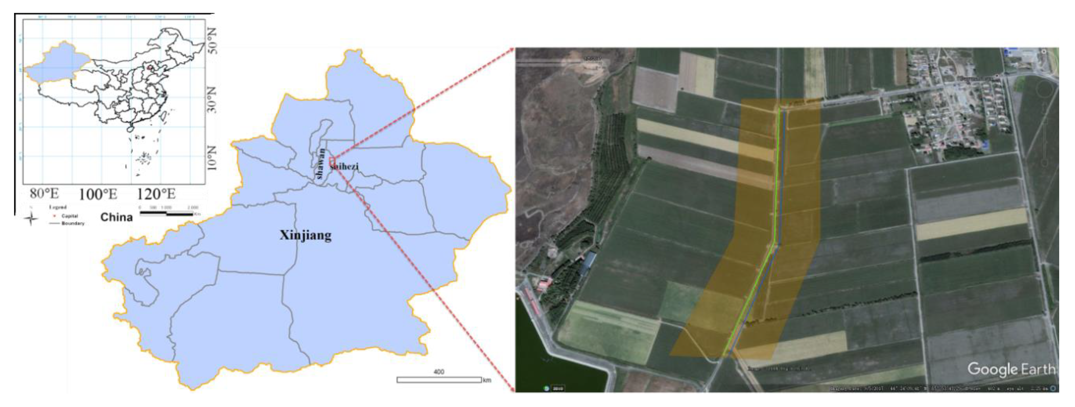
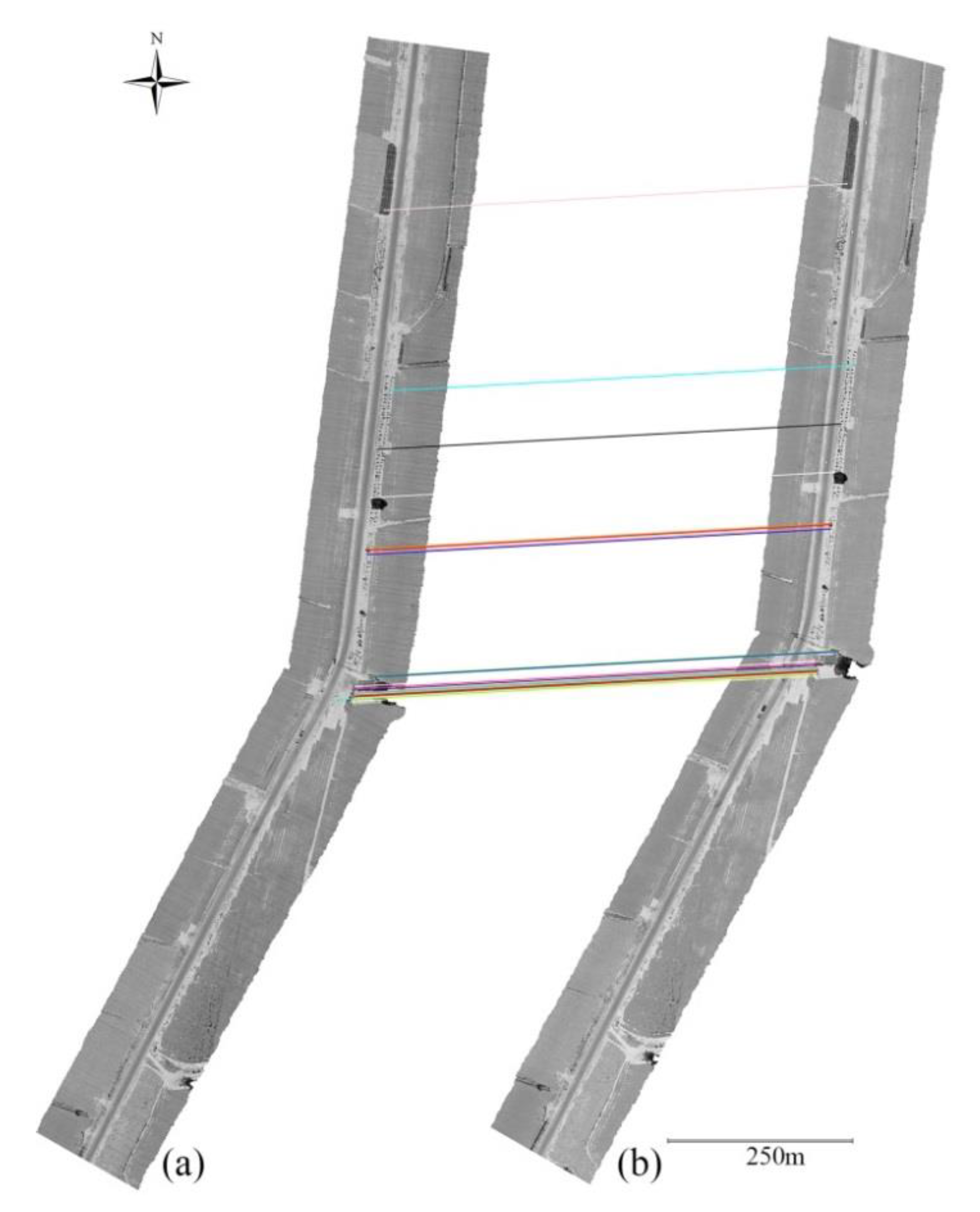
The study area is located in a farming area in the northwest of Shihezi city, Xinjiang, China (44°24′06″N, 85°53′41″E). The UAV LiDAR payload contains the OXTS xNAV550 GNSS/IMU dual-GNSS antenna navigation system and the RIEGL VUX-1UAV laser scanner, which were integrated on a Swiss-made ScoutB1-100 unmanned helicopter [26]. Detailed information of the payload is listed in Table 1. Time synchronization is based on GNSS provided by the GNSS/IMU unit, and the UAV LiDAR system flew above the experimental area on 29 July, 2017 with the proper flight configuration of planned flight lines (Figure 1). The laser scanner was set to a field angle of 110° with a scanning rate at 550 kHz. The UAV flew at a low altitude above ground level of 30 m and a cruising speed of 5 m/s, and captured two flight strips with opposite directions in the experiment. The point density for each scanning line is ~400–600 pts/m2 (Figure 2), the ground scanning width is ~85.7 m, and the spacing between the two flight trajectories is ~10 m. Each laser point attribute includes X, Y, and Z coordinates, the number of echoes at that point, scanning time, and laser intensity. In addition, the POS data of the strips can be derived from the inertial navigation system, including time, latitude, longitude, elevation, roll angle, pitch angle, and heading angle. These two data sets are the basic data sources for the following boresight angular error rectification.
2.2. Rectification of UAV LiDAR System Errors
2.2.1. LiDAR Georeferencing Equations
The geolocation error sources of a UAV LiDAR system usually include laser ranging error, GNSS positioning error, orientation angular error, lever arm error (displacements between laser scanner, IMU, and GNSS antenna), boresight angular error, and others. Among these errors, the boresight angular error and lever arm error belong to systematic errors, and the lever arm error can be measured by surveying instrument and usually has little effect on the accuracy of LiDAR point cloud data. However, the boresight angular error is usually caused by artificial factors or instable platform during the UAV LiDAR system installment stage prior to the flight. Although boresight angular error is not easy to be measured by surveying instruments, it can be estimated through a rigorous mathematic model. Based on the previous studies [20,22,27,28], the LiDAR georeferencing equation can be expressed as
where [XW YW ZW]T refers to the mapping frame coordinate of laser points; ρ denotes the distance measured by the laser scanner; [dx dy dz]T refers to the direction vector from the laser scanner center to GNSS antenna phase center, which can be measured by surveying instruments or obtained from the configuration file; [XW YG ZG]T refers to the mapping frame coordinate of GNSS antenna phase center; RL is a 3*3 rotation matrix that transforms the instantaneous scanning coordinate system into the scanning reference coordinate system, i.e., the current direction of laser pulse emission; RI is a 3*3 rotation matrix that transforms the scanner reference coordinate system into the IMU coordinate system; RN is a 3*3 rotation matrix that transforms the IMU coordinate system into the navigation coordinate system; and RW is a 3*3 rotation matrix that transforms the navigation system into the mapping frame coordinate system. Let
Then Equation (1) can be rewritten as
2.2.2. Boresight Alignment Model
The principle of boresight angular error rectification is based on the LiDAR georeferencing model and the laser scanning reference coordinate system with axes deviation error can be rectified by rotating to the real laser scanning reference coordinate system with three boresight angular corrections. If the boresight angular error parameters of the LiDAR system in three directions of rolling, pitching, and heading are ω, ϕ and κ, respectively, the rotation matrix derived from the boresight angular error in the three directions can be described as [29]
where, RM is the rotation matrix of the boresight angular error parameters. Considering that the boresight angular error parameter is usually small in number, Equation (3) can be approximated:
If we only consider the boresight angular error and ignore the other error sources, the LiDAR georeferencing equation can be described as
where [XW YW ZW]T denotes the coordinate of laser points in the mapping frame and RW and RN refer to the matrix that transforms navigation system into the mapping frame coordinate system and the matrix that transforms the IMU coordinate system into the navigation coordinate system, respectively. [XI YI ZI]T denotes the coordinate of laser points in IMU reference frame and [XG YG ZG]T denotes the coordinate of GNSS antenna phase center in the mapping frame. [dx dy dz]T refers to the direction vector from the laser scanner center to GNSS antenna phase center.
When P1 and P2 are two tie points, they should satisfy the following conditions.
where, [XW1 YW1 ZW1]T and [XW2 YW2 ZW2]T are the coordinate of tie points P1 and P2 in the mapping frame, respectively; [XI1 YI1 ZI1]T and [XI2 YI2 ZI2]T are the coordinate of tie points P1 and P2 in IMU reference frame, respectively; [XG1 YG1 ZG1]T and [XG2 YG2 ZG2]T are the coordinate of GNSS antenna phase center of tie points P1 and P2 in the mapping frame, respectively.
After applying the rectification model, conceptually, P1 and P2 would be the same point, which means
where RN1 and RN2 are matrixes that transform from the IMU coordinate system to the navigation coordinate system for tie points P1 and P2, respectively, and RM is the rotation matrix of the boresight angular error parameters. [Xtrue Ytrue Ztrue]T denotes the actual coordinate of tie points P1 and P2. Let
Then
In Equation (8), F is a nonlinear function and can be linearized by using the Taylor series expansion. F1 and F2 are the rectified coordinates of P1 and P2 in the mapping frame, respectively. If only the first-order term and the constant term remain, Equation (8) can be rewritten as
where, F0 represents the constant term that is an approximate value estimated using Equation (8) when RM is set with the initial value of boresight angular error parameters. Δω, Δϕ, and Δκ are the first-order terms.
Therefore, the observation error equation can be expressed as
where, V denotes the residual error matrix. If there are n pairs of tie points, then the observation error equation is
Equation (11) is given with the following notions.
Applying the least squares algorithm proposed by Marchant et al. [30], the solution of the Equation (11) is
Thus we can get the approximate solution of three unknown parameters: ∆ω, ∆φ, and ∆κ. Since only the first-order term of the Taylor expansion in Equation (9) is considered, we can solve the observation error equations in an iterative way, where the coefficient values and constant terms are modified successively till the observation error converges to a presetting threshold. Finally, the value of each unknown boresight angular error parameter can be obtained as follows
where ω, ϕ, and κ are the solution of the boresight angular error parameters, and ω0, ϕ0, and κ0 are the initial values of the boresight angular error parameters. Δωi, Δϕi, and Δκi represent the increment of the boresight angular error parameters at each iteration.
2.3. Automated Rectification Based on the Laser Intensity
When a UAV LiDAR system is used to scan terrain or targets over the scanned area, it can acquire the geospatial information and also record the reflection intensity of the scanned terrain and targets. The Rigel VUX-1LR laser scanner emits laser light pulses at the near-infrared wavelength centered at 1550nm. Due to the differences in the reflectivity of near-infrared laser light among different ground targets, the laser intensity may be helpful for feature points extraction and matching of the LiDAR flight strips. The Scale-Invariant Feature Transform (SIFT) algorithm [31] is more robust and ascendant in feature extraction and matching, but is only applicable for 2D image data. Therefore, we proposed a new approach, and the technical steps can be described as follows. First, the intensity of the point cloud data are interpolated to produce intensity images and the tie points are then retrieved based on the 2D adjacent intensity images, and based on the tie points in 2D intensity images, the tie points in 3D point cloud data can be also determined using a 2D-to-3D mapping strategy. After that, an observation error equation will be built based on the LiDAR georeferencing equation. The boresight angular error can be finally estimated by resolving the error equation using the extracted 3D tie point sets.
Because the distribution of laser points is spatially irregular and discrete, it is difficult to guarantee that the same ground point can be scanned in different scanning strips. Consequently, the tie points extracted from different LiDAR strips using SIFT algorithm are not real laser footprint points. This situation makes it difficult to obtain the corresponding observation information such as scanning time and POS data and, as a result, it becomes difficult or impossible to construct the LiDAR georeferencing equation. Considering there is a spatial constrained relationship between the tie points and their surrounded laser points, the K-nearest neighbor points of the tie points can be used as matching unit and an error equation can be constructed for every matching unit. The boresight angular error can then be solved iteratively and different flight lines can be aligned by applying the boresight angular error corrections.
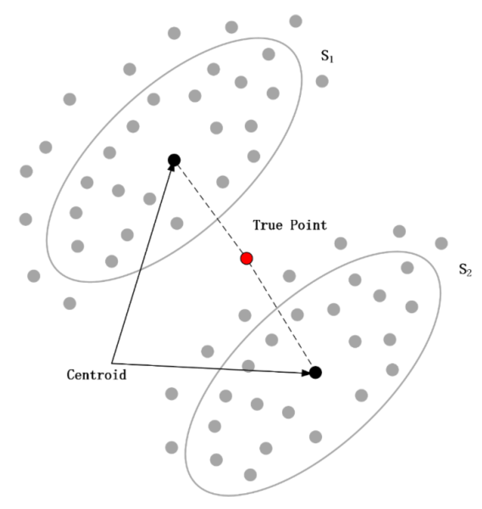
If the boresight angular error is not well rectified, the geolocations of the laser points might have spatial displacements, which cause tie points in adjacent flight strips to not be spatially coincident. As shown in Figure 3, S1 and S2 are the same area in the two adjacent UAV scanning strips, but the boresight angular error caused geolocation displacement, and the centroids in dark black color do not coincide spatially each other.
2.4. Workflow of Our Proposed Method
2.4.1. Generation of the Intensity Images
The laser point intensity data is to be transformed onto a horizontal plane and then rasterized, and each grid cell is assigned mean intensity value of all the laser points that fall into current grid cell. The resolution of the grid cell can be set as the average point spacing, as for some grid cells that have null value (i.e., hollow), the strategy is to find the nearest grid cell that is not more than two pixels apart and to assign the nearest grid cell value to this null grid cell, which can enable the intensity image to be more smoothly and homogeneously. Finally, the intensity image of each strip can be obtained after the processing abovementioned.
2.4.2. Tie Point Extraction in 2D Space
SIFT is robust for changes in illumination or viewing angle and shows a good strong potential in antinoise and is widely used in target tracking, image mosaic, etc. [32]. The SIFT algorithm was adopted in our study to extract the key points from the intensity image of each strip and obtain initial tie points by matching key points from the adjacent images. It is inevitable that there will be some pairs of pseudo matching points in the initial tie points, and thus, the RANSAC algorithm is used to optimize the initial tie points [33]. The local affine transformation invariance is used as a constraint between the adjacent strips to eliminate pseudo matching points.
2.4.3. Refining Tie Point Sets in 3D Space
The tie points retrieved from the intensity images are mapped to 3D point cloud space, and a K-neighborhood search algorithm was applied to find the K-nearest neighboring points in the 3D point cloud space. The resultant K-nearest points are considered as a tie point set or matching units among the different LiDAR scanning strips. The value of K needs to be determined according to terrain conditions and laser point spacing, so that the K-nearest neighboring points can be located on the same surface as much as possible to avoid 3D leap. Since we only consider the radiation characteristics of targets in the extraction of tie point sets and do not take into account the geometric characteristics inside the neighborhood of the tie points, as well as the influence of observation noise, some tie point sets can be found in areas with obvious radiation characteristics such as buildings edges and vegetation canopies. However, these tie point sets with unstable geometric features are more likely to cause matching errors, and need further optimization therefore. In our study, a 3D plane is fitted for each tie point set firstly, and then the normal angle between the pair of planes derived from the tie point set is calculated. The pairs of the tie points with a normal angle greater than a certain threshold δn and a height difference greater than a certain threshold δh will be eliminated and the optimized tie point sets can be achieved finally.
2.4.4. Estimation of Boresight Angular Error Parameters
Step 1: Assigning initial values
The initial values of boresight angular parameters are given based on prior knowledge, since the number of the boresight angular error parameters is relatively small, therefore the initial values of the three boresight angular parameters can be all set to 0.
Step 2: Construction of the observation error equation
For the tie point set in the n-th LiDAR scanning strip, if there is a point that is named in it, then the coordinate of the point in IMU coordinate system can be derived from Equation (1). Thus its corrected coordinate in the mapping frame coordinate system can be derived from Equation (5) with known boresight angular parameter values, and the centroid coordinate of the tie point set can be derived with following equation.
where n denotes the number of the UAV flightlines. The residual of the observation error equation is
We first calculate the unknown coefficient for each point of the tie point set, and then average the coefficients as the coefficient matrix of the normal equations with the following two equations.
If there are only two adjacent strips, only three observation error equations can be derived for each pair of tie points. For three or more LiDAR strips, three observation error equations can be listed between any two strips and then a total of 3*C2n equations will be derived.
Step 3: Solving observation error equations
There are three unknown parameters in the unknown matrix, since each pair of tie points can list three equations, so the boresight angular error can be solved using at least one pair of tie point set. Many pairs of tie point sets will cause redundant observations and form a complete observation error equation. The approximate solution to the boresight angular error is obtained by Equation (12) in this section, and the three boresight angular parameters are updated as follows
Step 4: Determining the termination of iterative running
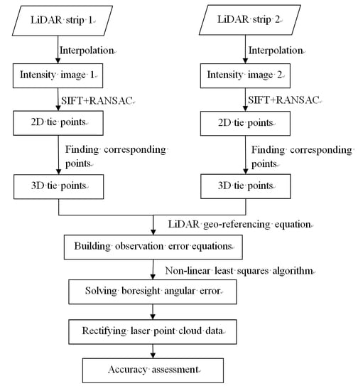
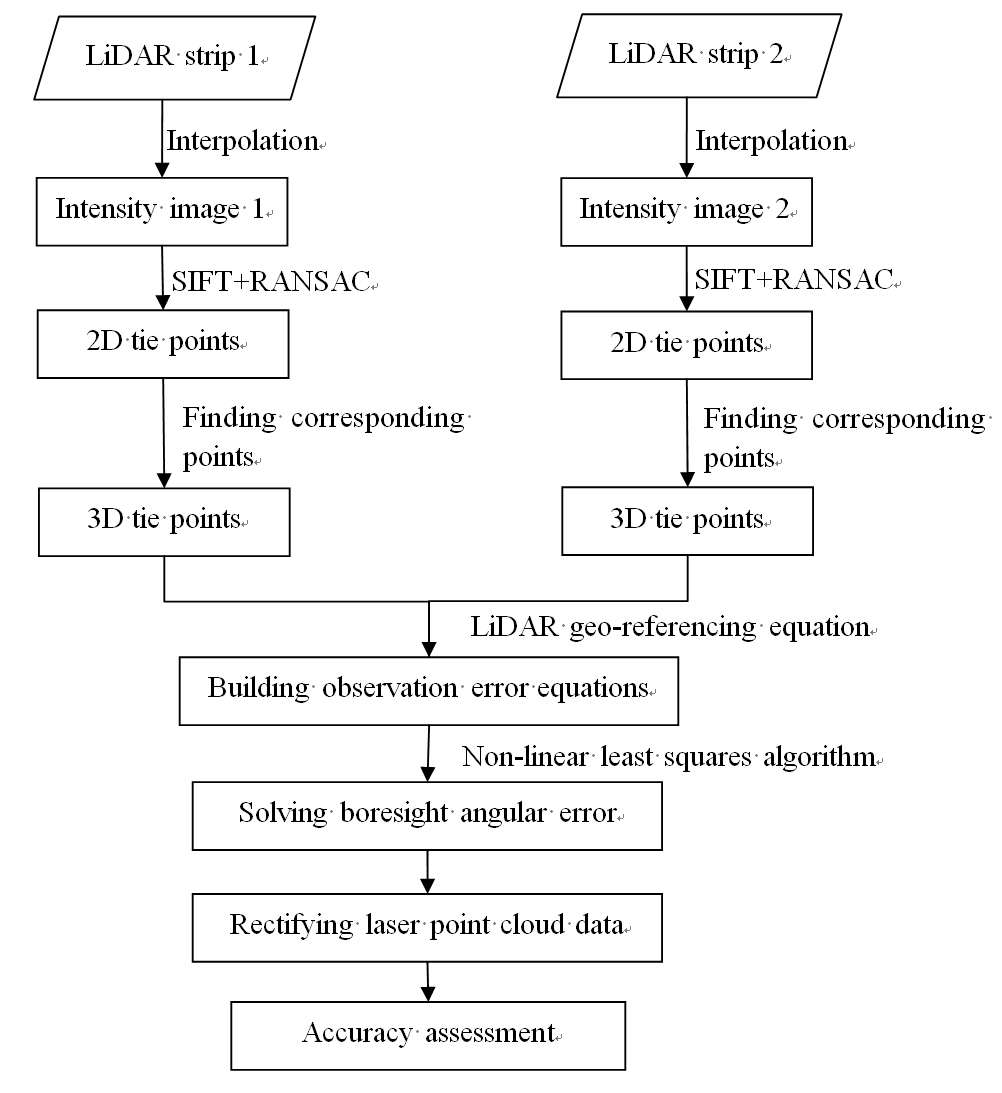
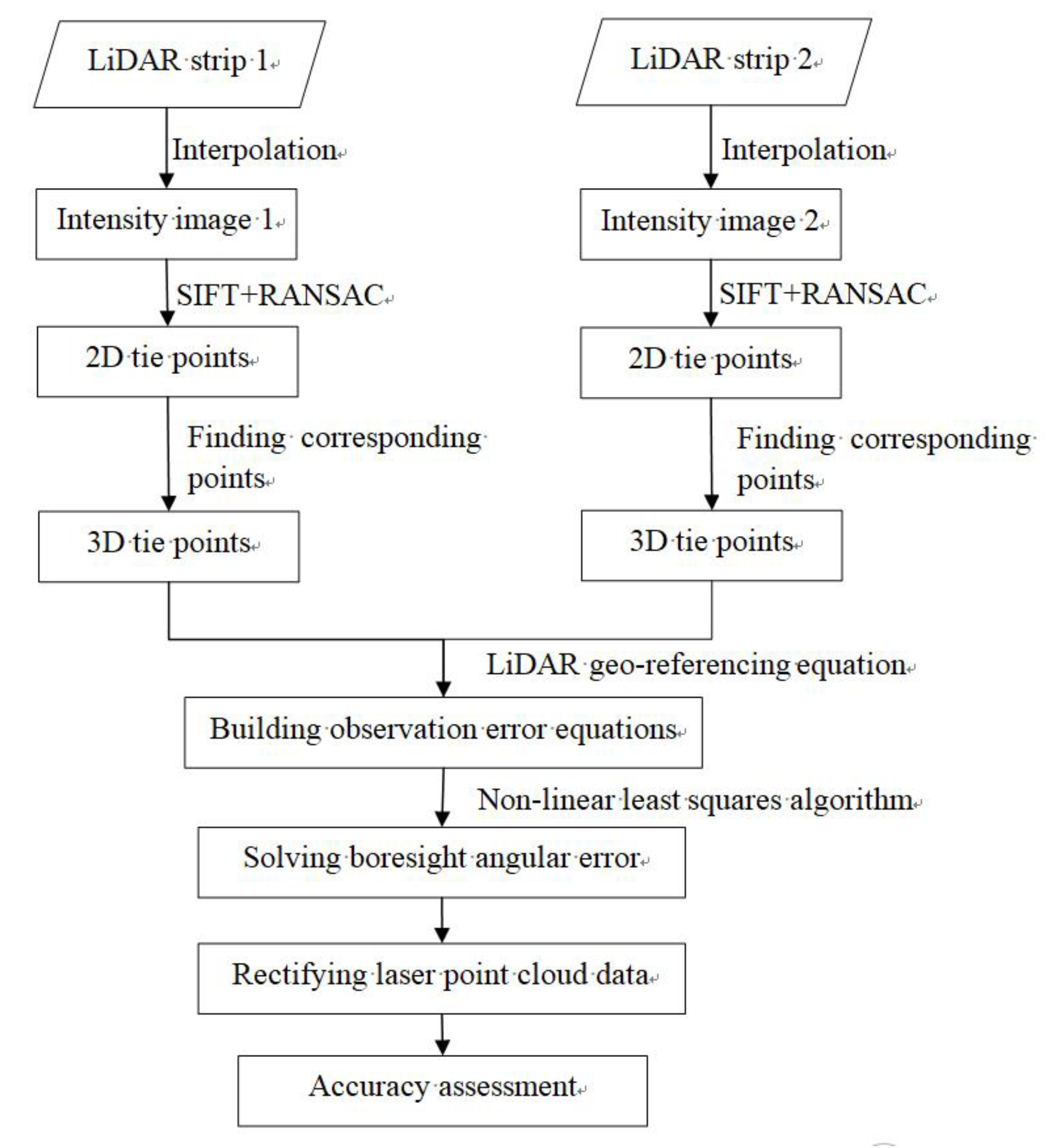
Whether the residual is convergent and whether the parameter value keeps almost unchanged is used as a termination condition of the iterative running. If both are satisfied, the iterative calculation will be stopped and the estimated values of the boresight angular parameters will be output. If both are not satisfied, then the current estimated parameter values will be set as new values of the boresight angular parameters of the next iteration, and go back to step 2 to continue the iterative running. The flowchart for the proposed method is illustrated in Figure 4.
In the implementation of the technical flowchart in our study, the 3D tie points were classified into two groups, the training set and testing set. The training samples were extracted from the total samples of 3D tie points in a random way, and the rest of the total samples were used as the testing samples. The training samples were applied to estimate the parameters for the boresight angular error while the testing ones were prepared for the verification of the model, and the disparity between the tie point pairs was adopted to be an index for measuring the model fitting effect. The random sample dividing operation were performed 100 times in the experiment to guarantee the best estimate of the model parameters, and finally the model parameters of the best verification were chosen to achieve robust and reliable estimation of the boresight angular error.
3. Results
3.1. 2D Tie Points Extraction in the Case Study
The two LiDAR strips’ data was captured with the RIEGL VUX-1UAV laser scanner onboard on a Swiss-made ScoutB1-100 unmanned helicopter on 29 July, 2017 were de-noised with an anomaly detector such as Gaussian distribution statistics model to remove the elevation anomaly points in a local neighborhood. After that, the intensity images were generated by interpolating the laser intensity data, and the SIFT algorithm was applied to detect feature points on the two intensity images. A 128-dimensional feature descriptor was generated using the SIFT algorithm to describe the local features of the key points such as position, scale, and rotation. Next, the Euclidean distance between the two descriptors was calculated and used as a similarity metric of the two-image matching points. The matching strategy is as follows. Take a given key point in the query image and find the key point that is closest to the target one based on the ranking of the similarity. A certain number of pairs of tie points of the two images were able to be extracted out from the 2D intensity images. The RANSAC algorithm was applied to remove pseudo matching pairs with the condition of affine invariance. Finally a total of 63 pairs of tie points were extracted with the SIFT algorithm and 23 pairs of refined tie points were remained after removing pseudo matching points. It can be seen that the tie points are mainly located near the flat ground and the edge of the buildings. The spatial distribution is relatively uniform and the link lines between all pairs of refined tie points are basically parallel and show a good consistency.
3.2. 3D Tie Point Sets Construction with the Two Flight Lines
Considering the flat topography in the study area and the spatial distribution of the tie point pairs in 2D space, the thresholding values of the normal vector angle parameter δn of the tie point set and the elevation range parameter δh of each point set were set to 30° and 0.5 m, respectively. In the transformation of the tie points from 2D to 3D, the value of the core parameter K has a great influence on the final results (for details see Section 4.1). After a series of experiments and comparisons in the selection of optimal tie points in 3D space, the best performance can be derived when K is set to 200, the discrepancy of the tie point set is the best and the standard deviation is the smallest at the same time. Therefore, the value of K is set to 200 to extract the tie point set in 3D space finally, and a total of 12 pairs of optimal 3D tie points were retrieved in the study (Figure 5).
3.3. Correction of the Boresight Angular Error of the Two Strips
The boresight angular errors of the Scount-100/RIEGL VUX-1UAV system were resolved with an automation workflow, in which only the POS data and laser point cloud data needed to be inputs. The operation for randomly creating the training set and testing set from the total 3D tie point samples were conducted 100 times in the experiment of this study. Each training set was used to train the model and estimate the parameters, and each testing one was used to verify the parameters. The training and testing sets that achieved the best estimation of the model parameters were adopted and the resultant estimation of the boresight angular error were used to correct the laser point cloud data of the two flight lines. To validate our proposed method, the data obtained by the commonly used stepwise geometric method [15] were used as a comparison. It can be seen in Table 2 that the values of the three boresight angular parameters are relatively small in number, almost within 1°, which is consistent with the results in previous studies.
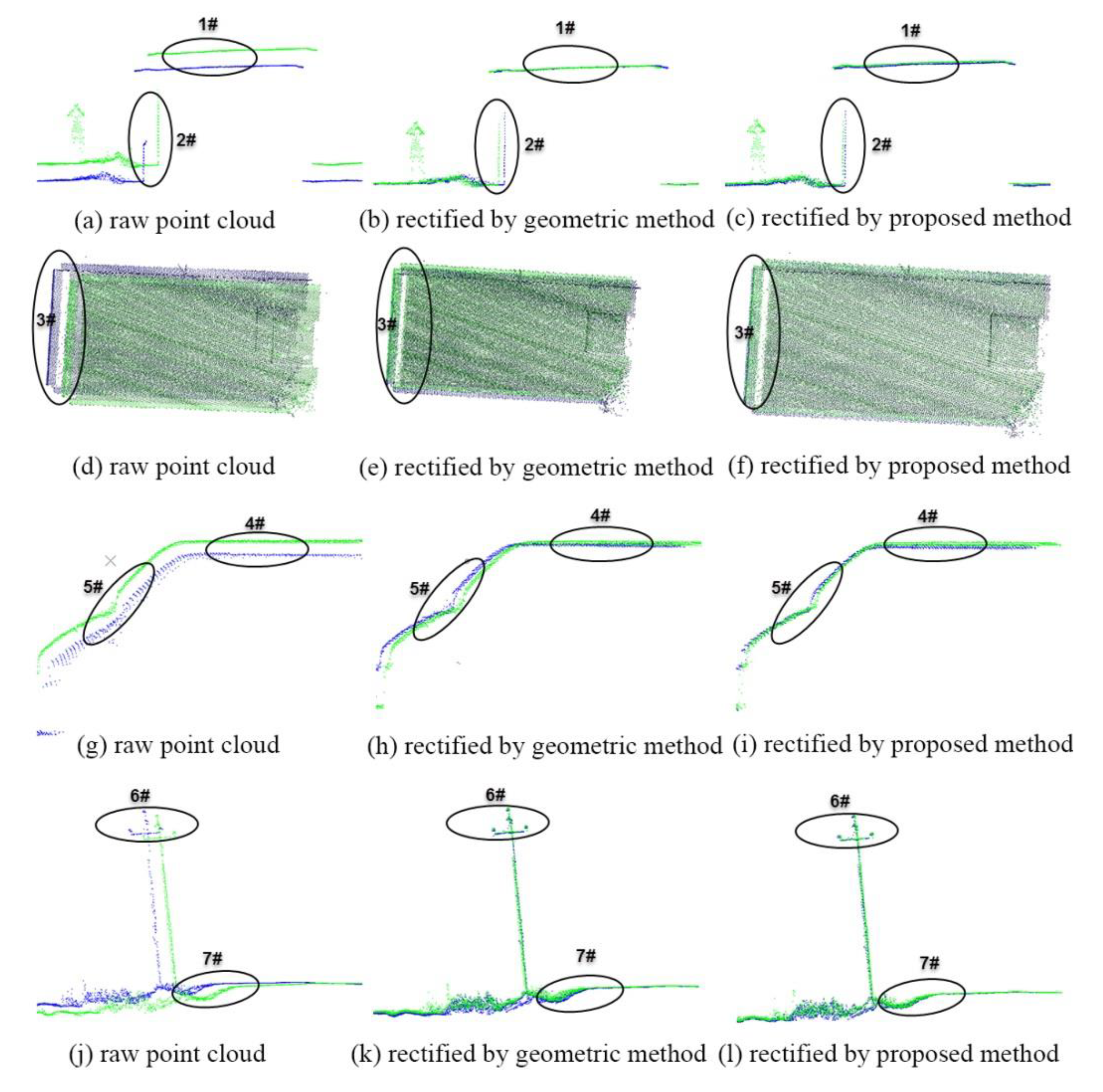
The resultant boresight angular error parameters were then substituted into Equation (5) to rectify the point cloud data of the two LiDAR scanning strips captured in Shihezi, Xinjiang, China on 29 July, 2017, and adjusted laser point data were achieved after the rectification using the parameters. A visual check of the corrections was illustrated in Figure 6, and it can be seen that the horizontal offset of the building facades have been effectively corrected after applying the rectification parameters.
Specifically it showed that our proposed method has a better performance than the stepwise geometric rectification method (e.g., 1# in Figure 6), but the stepwise geometric rectification method showed a slight better result in vertical direction (e.g., 2#). The displacement of the rooftop surfaces of the buildings were well aligned in horizontal direction and the rectification performance of the two methods showed few differences (e.g., 3#). The laser points of the vehicles have been well adjusted and became more coincident in the overlapping areas, and our proposed method slightly outperformed the stepwise geometric method (e.g., 4# and 5#). Because the diameter of the electricity poles is small and the spacing distance between the poles is relatively large, consequently, the rectification performance is not very distinct. However, the positional shift has been improved after the rectification (e.g., 6# and 7#). Generally speaking, our proposed method outperformed the stepwise geometric rectification method in most cases in this study, and has better automation and less ancillary data requirements such as GCPs, and thus can effectively improve the quality of laser point cloud data and enable good matching between adjacent flight lines.
3.4. Accuracy Assessment
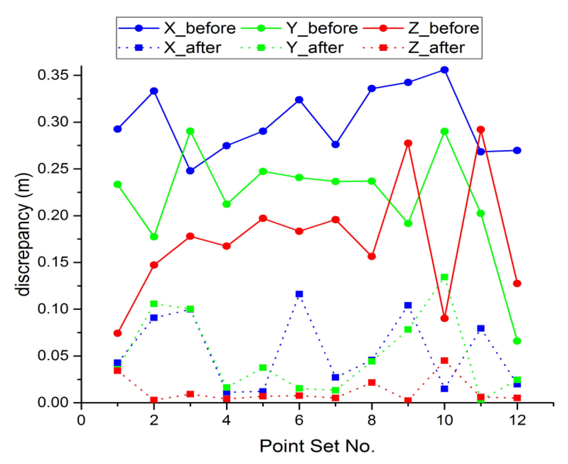
The effect of the boresight angular error rectification on the position of the tie point set was analyzed quantitatively by using the absolute coordinate deviation of the tie point set before and after rectification processing. In Figure 7, the X axis indicates the sequence number of the tie point set, and the Y axis represents the discrepancy of the centroid coordinates of the tie point set. On the whole, the discrepancy of the XYZ coordinate before the rectification is basically between 0.04 m and 0.35 m, and the discrepancy of the rectified XYZ coordinate is basically less than 0.1 m, which shows that after the rectification the offset error between the tie points was effectively corrected. In addition, the discrepancy of Z axis is significantly smaller than that of the XY axes, indicating the rectification performance in vertical direction is better than in horizontal directions.
Due to the lack of accurate ground control points in study area, the RMSE statistic is chosen to evaluate the rectification accuracy of all the laser point cloud data. The planar RMSE of the point cloud data was calculated by projecting vertical wall points into horizontal plane to form a series of discrete points, based on which, the fitted residual error was calculated. The elevation RMSE was also calculated by projecting the roof points to vertical plane to form a series of discrete points, and the standard deviation of elevation of these points was calculated. The rooftop and vertical walls of the buildings in the study area were selected as planar and vertical reference planes. Totally six vertical reference planes and six horizontal rooftop planes were selected in each flight strip to perform the accuracy assessment (Table 3).
It can be seen that after the rectification of boresight angular error, the accuracy in planar and elevation improved and the planar RMSE is 5.7 cm and decreases by 1.0 cm to 2.0 cm, while the elevation RMSE is ~1.4 cm and decreases by 0.5 cm to 1.0 cm. The RMSE reduction in elevation is slightly smaller than that in X–Y plane. In addition, our rectification method can achieve better correction in elevation than the stepwise geometric rectification method in the case study. As for the two LiDAR strips, the rectification of strip 1 is better than that of strip 2 in general.
4. Discussion
It can be seen in the case study that the proposed method can remove most of the boresight angular error caused by the unstable low-altitude UAV LiDAR system, and can achieve good matching of the two adjacent flight lines based on the laser intensity information. Compared to the stepwise geometric correction method, our method does not require any ground control points, feature objects, or raw observations of the laser scanner, and thus has larger degree of automation. However, the parameterization in our method may have influence on the final result, so we will discuss about it in the next subsections.
4.1. The Influence of Parameter K
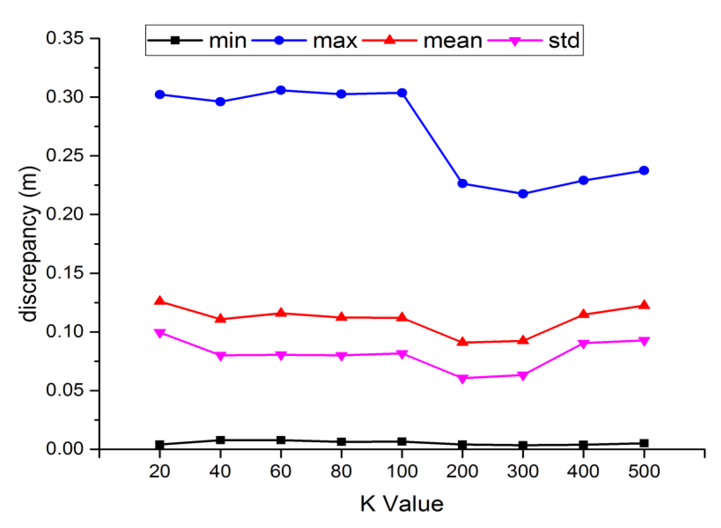
The K-nearest neighbor has a great impact on the spatial distribution of 3D tie points, and the proposed method requires extremely good quality tie point sets for accurately solving the error model. Thus, it is necessary to understand how K value influences on the final result. To empirically explore the influence of K, we selected a series of K values that fall between 0 and 500, and tried to resolve the parameters for the boresight angular error for each K value. Some results of the K values are shown in Table 4. It can be seen that the most sensitive parameter of the boresight angular error is κ, second ϕ, and third ω. Applying each solution under different K values to make a rectification for the tie point sets and the disparity statistical result is shown in Figure 8. It is found that regardless of the value of K, the minimum value of disparity tends to be 0 and shows little change. However, the maximum value of disparity is not stable, and shows an obvious trend of first increasing and then decreasing. The mean disparity seems to be stable and shows a general trend, decreasing first and followed by an increase, and reaches its minimum value when the K value is 200. The standard deviation of the disparity shows similar trends and reaches the minimum value when the K is 200. Empirically, the optimal value of K is determined by comparing the mean value and the standard deviation of disparity. Therefore, the rectification was processed with the optimal K value of 200.
4.2. The Influence of Calibration Parameter on Geolocation Error
Besides the K value, it is necessary to examine the influence of the boresight angular error on the positioning error of laser point cloud data quantitatively. Assuming that the remaining errors are all 0, according to the basic principle of laser point cloud geolocation, the influence of the boresight angular error parameters can be derived from the difference between Equation (5) and Equation (1), and is expressed in Equation (18).
where θ is the laser scanning angle; H is the altitude of the flight; ω, ϕ, and κ are boresight angular error parameters in three directions of rolling, pitching, and heading, respectively; and ρ denotes the distance measured by the laser scanner. It can be understood in Equation (18) that the geolocation error of a LiDAR system is proportional to the altitude H, and the higher the altitude is, the larger the planar and elevation error. When the laser scanning angle θ is constant, the pitching direction φ and heading direction κ together affect the X-direction error of the point cloud data, and the error increases with the increase of these two parameters. The rolling direction ω mainly affects the Y-direction and Z-direction errors of the point cloud data, and both are proportional to ω, and as the error increases, ω increases. It is worth noting that the scanning angle is also an important factor influencing the positioning error of the LiDAR system, and has only a direct effect on the X and Z direction errors of the laser point cloud data.
4.3. Influence of the Initial Values on Model Convergence
In addition to the parameters abovementioned, the convergence speed also has a significant impact on the practicability and robustness of the model for estimating the boresight angular error. Considering the assumption that the boresight angular error is relatively small in number, thus we preset the initial values of w, ϕ, and κ to zero, and the parameters of the boresight angular error can be solved after three iterations. If this is not true and the parameters are big in number, does the initial values of w, ϕ, and κ affect the convergence speed of the model? A series of initial values was preset and used to test the convergence speed (Table 5). It can be seen in Table 5 that the initial values of the boresight angular error parameters have slight influence on the convergence speed, and three or four iterations can achieve the convergence in our experiment. Even if the initial values were intentionally set to a very large value, i.e., 60°, the convergence can also be achieved only after six iterations. Therefore, empirically speaking, the initial values of the boresight angular error parameters have slight influence on the convergence speed. In other words, our proposed method is not sensitive to the initial values and possesses robustness and stability.
5. Conclusions
This paper presents a new method for the boresight angular error rectification of a UAV LiDAR system based on the laser intensity information. Our proposed method has been verified with tens of millions of laser point cloud data acquired by the Scount-100/RIEGL VUX-1UAV LiDAR system in a farmland located in the northwestern of Shihezi city, Xinjiang, China. A comparison with conventional stepwise geometric rectification method [15] was also conducted with the same data sets. It can be concluded that the boresight angular error is one of the main error sources leading to the positional error between different scanning strips of UAV LiDAR data. The boresight angular errors in the UAV LiDAR system used in our study were estimated by our proposed method, and the angular parameters are ω=-0.7385°, φ=-0.2245°, and κ=-0.7219°. After the rectification, the planar RMSE is 5.7 cm and decreased by 1.0 to 2.0 cm, and the elevation RMSE is 1.4 cm and decreased by 0.5 to 1.0 cm. It is also found that K value in K-nearest analysis has great influence on the estimation of the boresight angular error parameters. Due to the difficulty in the determination of a best K value theoretically, an empirical solution has been proposed in our study, simply put, it can be determined through comparing the rectification performance under a series of different K values. In this experiment, the best K value of 200 was adopted for the implementation of our proposed method, and can achieve best adjustment of the two LiDAR scanning strips. The sensitivity analysis of the angular parameters shows that ω is the weakest, followed by φ, and κ is the strongest. It should be noted that our proposed method is not sensitive to the initial values of ω, φ, and κ. In spite of different initial values, the resolving of the boresight angular error model can be accomplished in less than ten iterations. Thus our proposed method shows good robustness and stability in practice.
One limitation of this study is that the testing was just based on the two UAV LiDAR strips, and the experimental area is a relatively flat area and the main ground object types are vegetation and road pavement. Consequently, there is a potential uncertainty in the extraction of tie points. In the future, more validation work needs to be done on a larger dataset with more UAV flight lines. For example, testing work can be expanded to mining areas, built-up areas, and other regions with various topographical conditions and ground object types. In addition, in this paper we only considered the boresight angular error of the point cloud data, lacking of the analysis and comparison of other potential error sources. Future work will be focused on the combination of other error sources to design robust algorithms and make more improvement in the practicability of our proposed method.
Author Contributions
X.Z. conceived and designed the study, including preparation of the UAV LiDAR system, design of the methods, and English composition. R.G. designed and implemented the methods, analyzed the data, and performed the experiments. Q.S. collected in situ data as team leader and analyzed the data. J.C. designed the UAV flight paths and accomplished the data preprocessing.
Funding
This research was jointly funded by the National Natural Science Foundation of China, grant number 41571331 and by the Xinjiang Production and Construction Corps, grant numbers 2017DB005 & 2016AB001.
Acknowledgments
We would like to give our heartfelt thanks to the Xinjiang Corps Center for Geospatial Information Technology & Engineering Research for the support in the UAV flight and in situ data acquisition in Shihezi City, Xinjiang, China in July, 2017. We also want to extend our thanks to the anonymous reviewers for their valuable comments and suggestions that have improved our manuscript.
Conflicts of Interest
The authors declare no conflicts of interest.
References
- Chiang, K.W.; Tsai, G.J.; Li, Y.H.; El-Sheimy, N. Development of LiDAR-based UAV system for environment reconstruction. IEEE Geosci. Remote Sens. Lett. 2017, 14, 1790–1794. [Google Scholar] [CrossRef]
- Wallace, L.; Lucieer, A.; Watson, C.; Turner, D. Development of a UAV-LiDAR system with application to forest inventory. Remote Sens. 2012, 4, 1519. [Google Scholar] [CrossRef]
- Kaňuk, J.; Gallay, M.; Eck, C.; Zgraggen, C.; Dvorný, E. Technical Report: Unmanned Helicopter Solution for Survey-Grade Lidar and Hyperspectral Mapping. Pure Appl. Geophys. 2018, 175, 3357–3373. [Google Scholar] [CrossRef]
- Chen, C.F.; Li, Y.; Zhao, N.; Yan, C. Robust interpolation of DEMs from LiDAR-derived elevation data. IEEE Trans. Geosci. Remote Sens. 2018, 56, 1059–1068. [Google Scholar] [CrossRef]
- Lin, Y.; Hyyppä, J.; Jaakkola, A. Mini-UAV-borne LIDAR for fine-scale mapping. IEEE Geosci. Remote Sens. Lett. 2011, 8, 426–430. [Google Scholar] [CrossRef]
- Kwan, M.P.; Ransberger, D.M. LiDAR Assisted Emergency Response: Detection of Transport Network Obstructions Caused by Major Disasters. Comput. Environ. Urban Syst. 2010, 34, 179–188. [Google Scholar] [CrossRef]
- Hou, M.; Li, S.K.; Jiang, L.; Wu, Y.; Hu, Y.; Yang, S.; Zhang, X. A new method of gold foil damage detection in stone carving relics based on multi-temporal 3D LiDAR point clouds. ISPRS Int. J. Geo-Inf. 2016, 5, 60. [Google Scholar] [CrossRef]
- Guo, Q.; Su, Y.; Hu, T.; Zhao, X.; Wu, F.; Li, Y.; Liu, J.; Chen, L.; Xu, G.; Lin, G.; et al. An integrated UAV-borne lidar system for 3D habitat mapping in three forest ecosystems across China. Int. J. Remote Sens. 2017, 38, 2954–2972. [Google Scholar] [CrossRef]
- Sankey, T.; Donager, J.; McVay, J.; Sankey, J.B. UAV lidar and hyperspectral fusion for forest monitoring in the southwestern USA. Remote Sens. Environ. 2017, 195, 30–43. [Google Scholar] [CrossRef]
- Wieser, M.; Mandlburger, G.; Hollaus, M.; Otepka, J.; Glira, P.; Pfeifer, N. A case study of UAS borne laser scanning for measurement of tree stem diameter. Remote Sens. 2017, 9, 1154. [Google Scholar] [CrossRef]
- Falkowski, M.J.; Evans, J.S.; Martinuzzi, S.; Gessler, P.E.; Hudak, A.T. Characterizing forest succession with LiDAR data: An evaluation for the inland northwest, USA. Remote Sens. Environ. 2009, 113, 946–956. [Google Scholar] [CrossRef]
- Díaz-Varela, R.A.; De la Rosa, R.; León, L.; Zarco-Tejada, P.J. High-resolution airborne UAV imagery to assess olive tree crown parameters using 3d photo reconstruction: Application in breeding trials. Remote Sens. 2015, 7, 4213–4232. [Google Scholar] [CrossRef]
- Dan, J.; Yang, X.; Shi, Y.; Guo, Y. Random Error Modeling and Analysis of Airborne LiDAR Systems. Remote Sens. 2014, 52, 3885–3894. [Google Scholar]
- Glennie, C. Rigorous 3D error analysis of kinematic scanning LIDAR systems. J. Appl. Geod. 2007, 1, 147–157. [Google Scholar] [CrossRef]
- Zhang, Y.; Xiong, X.; Zheng, M.; Huang, X. LiDAR strip adjustment using multi-features matched with aerial images. IEEE Trans. Geosci. Remote Sens. 2015, 53, 976–987. [Google Scholar] [CrossRef]
- Hebel, M.; Stilla, U. Simultaneous calibration of ALS systems and alignment of multiview LiDAR scans of urban areas. IEEE Trans. Geosci. Remote Sens. 2012, 50, 2364–2379. [Google Scholar] [CrossRef]
- Li, F.; Cui, X.; Liu, X.; Wei, A.; Wu, Y. Positioning errors analysis on airborne LIDAR point clouds. Infrared Laser Eng. 2014, 43, 1842–1849. [Google Scholar]
- Skaloud, J.; Lichti, D. Rigorous approach to boresight self-calibration in airborne laser scanning. ISPRS J. Photogramm. Remote Sens. 2006, 61, 47–59. [Google Scholar] [CrossRef]
- Bang, K.I.; Habib, A.; Kersting, A. Estimation of Biases in LiDAR System Calibration Parameters Using Overlapping Strips. Can. J. Remote Sens. 2010, 36, S335–S354. [Google Scholar] [CrossRef]
- Habib, A.; Kersting, A.P.; Bang, K.I.; Lee, D. Alternative methodologies for the internal quality control of parallel LiDAR strips. Canadian 2010, 48, 221–236. [Google Scholar] [CrossRef]
- Colomina, I.; Molina, P. Unmanned aerial systems for photogrammetry and remote sensing: A review. ISPRS J. Photogramm. Remote Sens. 2014, 92, 79–97. [Google Scholar] [CrossRef] [Green Version]
- Filin, S. Elimination of systematic errors from airborne laser scanning data. In Proceedings of the 2005 IEEE International Geoscience and Remote Sensing Symposium, Seoul, Korea, 25–29 July 2005. [Google Scholar]
- Rodarmel, C.; Lee, M.; Gilbert, J.; Wilkinson, B.; Theiss, H.; Dolloff, J.; O’Neill, C. The universal LiDAR error model. Photogramm. Eng. Remote Sens. 2015, 81, 543–556. [Google Scholar] [CrossRef]
- Zhang, X.; Forsberg, R. Retrieval of Airborne LiDAR misalignments based on the stepwise geometric method. Surv. Rev. 2010, 42, 176–192. [Google Scholar] [CrossRef]
- Le Scouarnec, R.; Touzé, T.; Lacambre, J.B.; Seube, N. A new reliable boresight calibration method for mobile laser scanning applications. ISPRS Int. Arch. Photogramm. Remote Sens. Spat. Inf. Sci. 2014, 40, 67–72. [Google Scholar] [CrossRef]
- Gallay, M.; Eck, C.; Zgraggen, C.; Kaňuk, J.; Dvorný, E. High resolution airborne laser scanning and hyperspectral imaging with a small UAV platform. ISPRS Int. Arch. Photogramm. Remote Sens. Spat. Inf. Sci. 2016, 41, 823–827. [Google Scholar] [CrossRef]
- Filin, S. Recovery of systematic biases in laser altimetry data using natural surfaces. Photogramm. Eng. Remote Sens. 2003, 69, 1235–1242. [Google Scholar] [CrossRef]
- Schenk, T. Modeling and Analyzing Systematic Errors of Airborne Laser Scanners; Technical Notes in Photogrammetry; The Ohio State University: Columbus, OH, USA, 2001. [Google Scholar]
- Bäumker, M.; Heimes, F.J. New Calibration and computing method for direct georeferencing of image and scanner data using the position and angular data of a hybrid inertial navigation system. Proc. Natl. Acad. Sci. USA 2001, 97, 14560–14565. [Google Scholar]
- Marchant, C.C.; Moon, T.K.; Jacob, H.G. An Iterative Least Square Approach to Elastic-Lidar Retrievals for Well-Characterized Aerosols. IEEE Trans. Geosci. Remote Sens. 2010, 48, 2430–2444. [Google Scholar] [CrossRef]
- Lowe, D.G. Distinctive image features from scale-invariant key points. Int. J. Comput. Vis. 2004, 60, 91–110. [Google Scholar] [CrossRef]
- Wang, F.B.; Tu, P.; Wu, C.; Chen, L.; Feng, D. Multi-image mosaic with sift and vision measurement for microscale structures processed by femtosecond laser. Opt. Lasers Eng. 2018, 100, 124–130. [Google Scholar] [CrossRef]
- Guo, B.; Li, Q.; Huang, X.; Wang, C. An improved method for power-line reconstruction from point cloud data. Remote Sens. 2016, 8, 36. [Google Scholar] [CrossRef]
Figure 1.
Geographic location of the study area and the unmanned aerial vehicle (UAV) flight strips acquired in the experiment; the green and blue lines in the right image indicate the two flight lines.
Figure 1.
Geographic location of the study area and the unmanned aerial vehicle (UAV) flight strips acquired in the experiment; the green and blue lines in the right image indicate the two flight lines.

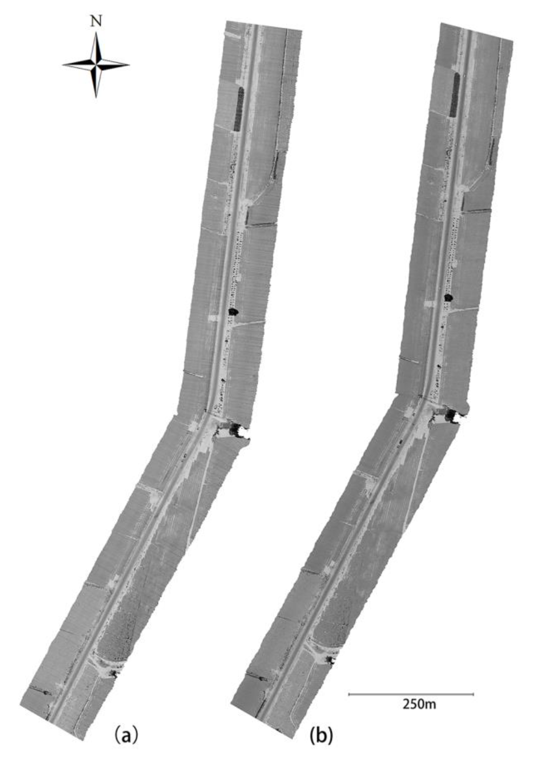
Figure 2.
Point cloud derived from the two flight strips from south to north (a) and from north to south (b). The laser point density for each scanning line is ~400–600 pts/m2.
Figure 2.
Point cloud derived from the two flight strips from south to north (a) and from north to south (b). The laser point density for each scanning line is ~400–600 pts/m2.

Figure 3.
Sketch map of positional displacement caused by the boresight angle error. The two centroids in dark black color should be coincident and the same point with the red one if there is no boresight angular error.
Figure 3.
Sketch map of positional displacement caused by the boresight angle error. The two centroids in dark black color should be coincident and the same point with the red one if there is no boresight angular error.

Figure 4.
Flowchart for the proposed method with two experimental UAV LiDAR flight strips.

Figure 5.
The tie point pairs by transforming the tie points from 2D to 3D space. The two intensity images were generated from the intensity of the flight strips captured from south to north (a) and from north to south (b).
Figure 5.
The tie point pairs by transforming the tie points from 2D to 3D space. The two intensity images were generated from the intensity of the flight strips captured from south to north (a) and from north to south (b).

Figure 6.
(a–l) Visual check of the performance of the laser point cloud data after the rectification with the proposed method in this study and the stepwise geometric method found in the literature [15].
Figure 6.
(a–l) Visual check of the performance of the laser point cloud data after the rectification with the proposed method in this study and the stepwise geometric method found in the literature [15].

Figure 7.
Absolute deviations between sets of tie points before and after boresight angular error correction. The x-axis indicates the sequence number of the tie point set and the y-axis represents the discrepancy of the centroid coordinates of the tie point set.
Figure 7.
Absolute deviations between sets of tie points before and after boresight angular error correction. The x-axis indicates the sequence number of the tie point set and the y-axis represents the discrepancy of the centroid coordinates of the tie point set.

Figure 8.
The disparity of the 3D tie point sets with different K values. The K value of 200 is recognized as the proper value that can achieve smallest mean geolocation disparity.
Figure 8.
The disparity of the 3D tie point sets with different K values. The K value of 200 is recognized as the proper value that can achieve smallest mean geolocation disparity.


Table 1.
The core specifications of the UAV Light and Detection Ranging (LiDAR) system.
| Laser Scanner1 | Specifications | GNSS/IMU2 | Specifications |
|---|---|---|---|
| Minimum Range | 5 m | Positioning Mode | RTK |
| Pulse Repetition Rate | 550 KHz | Data Frequency | 100 Hz |
| Measurement Accuracy | 0.015 m | Position Accuracy(CEP) | H:0.02 m; V:0.03 m |
| Scanning Speed | 200 scan/s | Speed Accuracy | 0.1 km/h |
| Angle Resolution | 0.001° | Roll Accuracy (1σ) | 0.05° |
| Field of View | 330° | Pitch Accuracy (1σ) | 0.05° |
| Echo Signal Intensity | 16 bit | Heading Accuracy (1σ) | 0.10° |
Table 2.
Estimated boresight angle error parameters.
| Method | Stepwise Geometric Method | Our Proposed Method | ||||
|---|---|---|---|---|---|---|
| Parameter | ω | ϕ | κ | ω | ϕ | κ |
| Estimated value | −1.050° | −0.2580° | −0.7980° | −0.7384° | −0.2245° | −0.7219° |
Table 3.
Accuracy assessment based on all the laser points.
| Error | Planar RMSE/m | Elevation RMSE/m | ||||
|---|---|---|---|---|---|---|
| Method | Raw data | Stepwise geometric method | Proposed method | Raw data | Step-wise geometric method | Proposed method |
| Strip 1 | 0.060 | 0.049 | 0.050 | 0.024 | 0.015 | 0.014 |
| Strip 2 | 0.075 | 0.059 | 0.064 | 0.020 | 0.015 | 0.014 |
| Average | 0.068 | 0.054 | 0.057 | 0.022 | 0.015 | 0.014 |
Table 4.
The boresight angle errors of different K values.
| K value | Match count | ω/° | ϕ/° | κ/° |
|---|---|---|---|---|
| 20 | 13 | -0.7302 | -0.3353 | -2.3283 |
| 40 | 12 | -0.7366 | -0.2530 | -1.1801 |
| 60 | 12 | -0.7384 | -0.2507 | -1.1319 |
| 80 | 12 | -0.7373 | -0.2451 | -1.0975 |
| 100 | 12 | -0.7395 | -0.2382 | -0.9498 |
| 200 | 12 | -0.7384 | -0.2245 | -0.7219 |
| 300 | 11 | -0.7492 | -0.2951 | -1.6186 |
| 400 | 11 | -0.7500 | -0.2955 | -1.6275 |
| 500 | 10 | -0.7498 | -0.2490 | -1.6450 |
Table 5.
The relationship between the convergence speed and the initial values.
| Initial Value | Iteration Count | Converges to Same Value | ||
|---|---|---|---|---|
| ω/° | ϕ/° | κ/° | ||
| 0 | 0 | 0 | 3 | — |
| 10 | 0 | 0 | 4 | yes |
| 0 | 10 | 0 | 3 | yes |
| 0 | 0 | 10 | 3 | yes |
| 10 | 10 | 0 | 3 | yes |
| 10 | 0 | 10 | 3 | yes |
| 0 | 10 | 10 | 4 | yes |
| 10 | 10 | 10 | 4 | yes |
| 30 | 30 | 30 | 4 | yes |
| 60 | 60 | 60 | 6 | yes |
© 2019 by the authors. Licensee MDPI, Basel, Switzerland. This article is an open access article distributed under the terms and conditions of the Creative Commons Attribution (CC BY) license (http://creativecommons.org/licenses/by/4.0/).
Share and Cite
MDPI and ACS Style
Zhang, X.; Gao, R.; Sun, Q.; Cheng, J. An Automated Rectification Method for Unmanned Aerial Vehicle LiDAR Point Cloud Data Based on Laser Intensity. Remote Sens. 2019, 11, 811. https://0-doi-org.brum.beds.ac.uk/10.3390/rs11070811
AMA Style
Zhang X, Gao R, Sun Q, Cheng J. An Automated Rectification Method for Unmanned Aerial Vehicle LiDAR Point Cloud Data Based on Laser Intensity. Remote Sensing. 2019; 11(7):811. https://0-doi-org.brum.beds.ac.uk/10.3390/rs11070811
Chicago/Turabian StyleZhang, Xianfeng, Renqiang Gao, Quan Sun, and Junyi Cheng. 2019. "An Automated Rectification Method for Unmanned Aerial Vehicle LiDAR Point Cloud Data Based on Laser Intensity" Remote Sensing 11, no. 7: 811. https://0-doi-org.brum.beds.ac.uk/10.3390/rs11070811
Note that from the first issue of 2016, this journal uses article numbers instead of page numbers. See further details here.