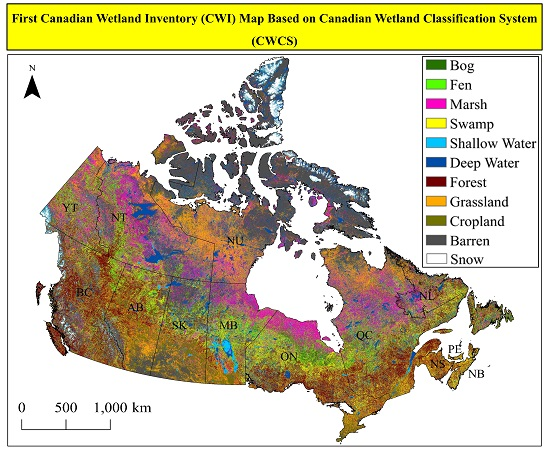
Canadian Wetland Inventory using Google Earth Engine: The First Map and Preliminary Results

 ,
,  ,
,  ,
,  , ,
, ,
Abstract
:
1. Introduction
2. Study Area and Datasets
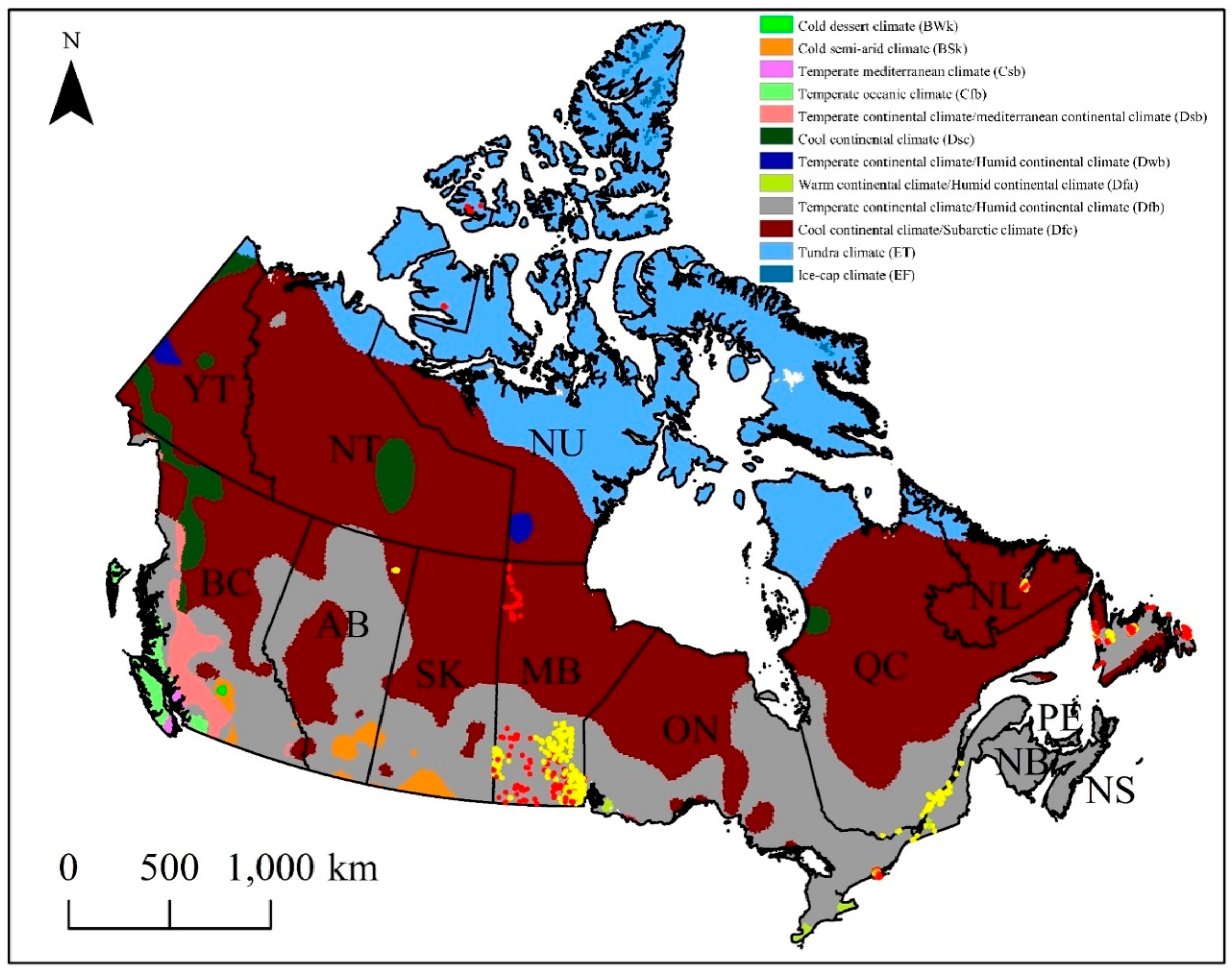
2.1. Study Area
2.2. Field Data
2.3. Satellite Data
3. Methodology
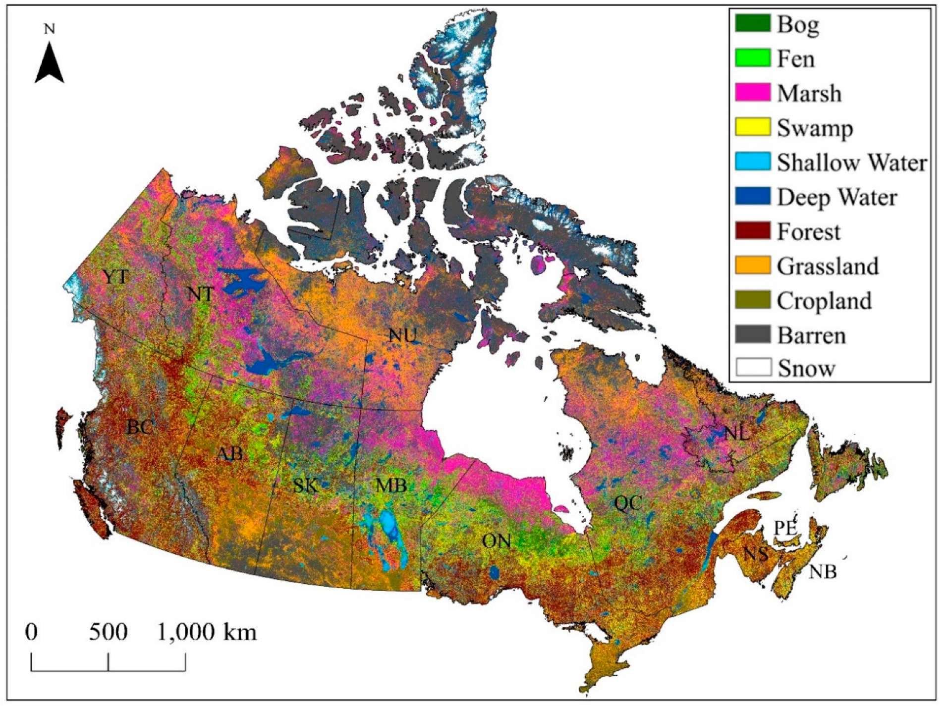
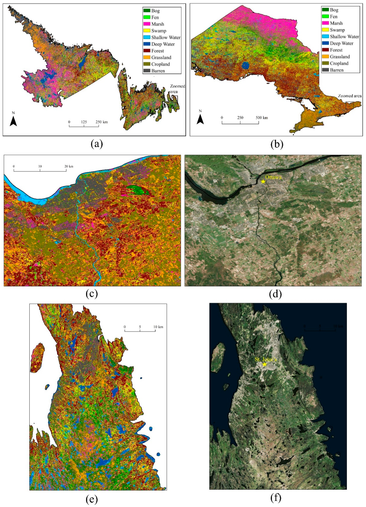
4. Results
5. Discussion
5.1. Wetland Complexity
5.2. Field Data
5.3. Satellite Data
5.4. Input Features
5.5. Classification Method
5.6. Merging/Splitting Non-Wetland Classes
5.7. Estimated Wetland Areas
5.8. Wetland Change Detection
5.9. GEE Limitations
5.10. Contribution in Other Fields
5.11. Global Wetland Mapping
6. Conclusions
Author Contributions
Funding
Acknowledgments
Conflicts of Interest
References
- Mahdavi, S.; Salehi, B.; Granger, J.; Amani, M.; Brisco, B.; Huang, W. Remote sensing for wetland classification: A comprehensive review. GISci. Remote Sens. 2018, 55, 623–658. [Google Scholar] [CrossRef]
- Marton, J.M.; Creed, I.F.; Lewis, D.B.; Lane, C.R.; Basu, N.B.; Cohen, M.J.; Craft, C.B. Geographically isolated wetlands are important biogeochemical reactors on the landscape. Bioscience 2015, 65, 408–418. [Google Scholar] [CrossRef]
- Carter, V. An overview of the hydrologic concerns related to wetlands in the United States. Can. J. Bot. 1986, 64, 364–374. [Google Scholar] [CrossRef]
- Fisher, J.; Acreman, M. Wetland nutrient removal: A review of the evidence. Hydrol. Earth Syst. Sci. Discus. 2004, 8, 673–685. [Google Scholar] [CrossRef]
- Hey, D.L.; Kostel, J.A.; Crumpton, W.G.; Mitsch, W.J.; Scott, B. The roles and benefits of wetlands in managing reactive nitrogen. J. Soil Water Conserv. 2012, 67, 47A–53A. [Google Scholar] [CrossRef]
- Kingsford, R.T.; Basset, A.; Jackson, L. Wetlands: conservation’s poor cousins. Aquat. Conserv. Mar. Freshw. Ecosyst. 2016, 26, 892–916. [Google Scholar] [CrossRef]
- Amani, M.; Salehi, B.; Mahdavi, S.; Granger, J.; Brisco, B. Wetland classification in Newfoundland and Labrador using multi-source SAR and optical data integration. GISci. Remote Sens. 2017, 54, 779–796. [Google Scholar] [CrossRef]
- Secretariat, R.C. Ramsar Handbooks for the Wise Use of Wetlands; Ramsar Convention Secretariat: Gland, Switzerland, 2007. [Google Scholar]
- Ozesmi, S.L.; Bauer, M.E. Satellite remote sensing of wetlands. Wetl. Ecol. Manag. 2002, 10, 381–402. [Google Scholar] [CrossRef]
- Wulder, M.; Li, Z.; Campbell, E.; White, J.; Hobart, G.; Hermosilla, T.; Coops, N. A National Assessment of Wetland Status and Trends for Canada’s Forested Ecosystems Using 33 Years of Earth Observation Satellite Data. Remote Sens. 2018, 10, 1623. [Google Scholar] [CrossRef]
- Mahdavi, S.; Salehi, B.; Amani, M.; Granger, J.E.; Brisco, B.; Huang, W.; Hanson, A. Object-based classification of wetlands in Newfoundland and Labrador using multi-temporal PolSAR data. Can. J. Remote Sens. 2017, 43, 432–450. [Google Scholar] [CrossRef]
- Amani, M.; Salehi, B.; Mahdavi, S.; Granger, J.E.; Brisco, B.; Hanson, A. Wetland classification using multi-source and multi-temporal optical remote sensing data in Newfoundland and Labrador, Canada. Can. J. Remote Sens. 2017, 43, 360–373. [Google Scholar] [CrossRef]
- Montgomery, J.; Brisco, B.; Chasmer, L.; Devito, K.; Cobbaert, D.; Hopkinson, C. SAR and Lidar Temporal Data Fusion Approaches to Boreal Wetland Ecosystem Monitoring. Remote Sens. 2019, 11, 161. [Google Scholar] [CrossRef]
- DeLancey, E.R.; Kariyeva, J.; Cranston, J.; Brisco, B. Monitoring hydro temporal variability in Alberta, Canada with multi-temporal Sentinel-1 SAR data. Can. J. Remote Sens. 2018, 44, 1–10. [Google Scholar] [CrossRef]
- Fournier, R.A.; Grenier, M.; Lavoie, A.; Hélie, R. Towards a strategy to implement the Canadian Wetland Inventory using satellite remote sensing. Can. J. Remote Sens. 2007, 33, S1–S16. [Google Scholar] [CrossRef]
- National Wetlands Working Group. The Canadian Wetland Classification System, 2nd ed.; Warner, B.G., Rubec, C.D.A., Eds.; National Wetlands Working Group, Wetlands Research Branch, University of Waterloo: Waterloo, ON, Canada, 1997. [Google Scholar]
- White, L.; Millard, K.; Banks, S.; Richardson, M.; Pasher, J.; Duffe, J. Moving to the RADARSAT constellation mission: Comparing synthesized compact polarimetry and dual polarimetry data with fully polarimetric RADARSAT-2 data for image classification of peatlands. Remote Sens. 2017, 9, 573. [Google Scholar] [CrossRef]
- Brisco, B.; Ahern, F.; Murnaghan, K.; White, L.; Canisus, F.; Lancaster, P. Seasonal change in wetland coherence as an aid to wetland monitoring. Remote Sens. 2017, 9, 158. [Google Scholar] [CrossRef]
- Ahern, F.; Brisco, B.; Murnaghan, K.; Lancaster, P.; Atwood, D.K. Insights Into Polarimetric Processing for Wetlands From Backscatter Modeling and Multi-Incidence Radarsat-2 Data. IEEE J. Sel. Top. Appl. Earth Obs. Remote Sens. 2018, 11, 3040–3050. [Google Scholar] [CrossRef]
- Amani, M.; Salehi, B.; Mahdavi, S.; Brisco, B.; Shehata, M. A Multiple Classifier System to improve mapping complex land covers: A case study of wetland classification using SAR data in Newfoundland, Canada. Int. J. Remote Sens. 2018, 39, 7370–7383. [Google Scholar] [CrossRef]
- Gorelick, N.; Hancher, M.; Dixon, M.; Ilyushchenko, S.; Thau, D.; Moore, R. Google Earth Engine: Planetary-scale geospatial analysis for everyone. Remote Sens. Environ. 2017, 202, 18–27. [Google Scholar] [CrossRef]
- Kumar, L.; Mutanga, O. Google Earth Engine Applications Since Inception: Usage, Trends, and Potential. Remote Sens. 2018, 10, 1509. [Google Scholar] [CrossRef]
- Dong, J.; Xiao, X.; Menarguez, M.A.; Zhang, G.; Qin, Y.; Thau, D.; Biradar, C.; Moore III, B. Mapping paddy rice planting area in northeastern Asia with Landsat 8 images, phenology-based algorithm and Google Earth Engine. Remote Sens. Environ. 2016, 185, 142–154. [Google Scholar] [CrossRef] [Green Version]
- Chen, B.; Xiao, X.; Li, X.; Pan, L.; Doughty, R.; Ma, J.; Dong, J.; Qin, Y.; Zhao, B.; Wu, Z. A mangrove forest map of China in 2015: Analysis of time series Landsat 7/8 and Sentinel-1A imagery in Google Earth Engine cloud computing platform. ISPRS J. Photogramm. Remote Sens. 2017, 131, 104–120. [Google Scholar] [CrossRef]
- Xiong, J.; Thenkabail, P.; Tilton, J.; Gumma, M.; Teluguntla, P.; Oliphant, A.; Congalton, R.; Yadav, K.; Gorelick, N. Nominal 30-m cropland extent map of continental Africa by integrating pixel-based and object-based algorithms using Sentinel-2 and Landsat-8 data on Google Earth Engine. Remote Sens. 2017, 9, 1065. [Google Scholar] [CrossRef]
- Environment and Climate Change Canada. Available online: https://www.canada.ca/en/environment-climate-change/services/environmental-indicators/extent-wetlands.html (accessed on 15 February 2019).
- Real Time Water Quality Monitoring Workshop (2018). Available online: https://www.mae.gov.nl.ca/waterres/rti/rtwq/workshops.html#2018 (accessed on 10 December 2018).
- Environment and Climate Change Canada. Canadian Environmental Sustainability Indicators: Extent of Canada’s Wetlands. Available online: www.ec.gc.ca/indicateurs-indicators/default.asp?lang=en&n=69E2D25B-1 (accessed on 15 February 2019).
- Kottek, M.; Grieser, J.; Beck, C.; Rudolf, B.; Rubel, F. World map of the Köppen-Geiger climate classification updated. Meteorol. Z. 2006, 15, 259–263. [Google Scholar] [CrossRef]
- Amani, M.; Salehi, B.; Mahdavi, S.; Brisco, B. Spectral analysis of wetlands using multi-source optical satellite imagery. ISPRS J. Photogramm. Remote Sens. 2018, 144, 119–136. [Google Scholar] [CrossRef]
- Breiman, L. Random forests. Mach. Learn. 2001, 45, 5–32. [Google Scholar] [CrossRef]
- Hermosilla, T.; Wulder, M.A.; White, J.C.; Coops, N.C.; Hobart, G.W. Disturbance-informed annual land cover classification maps of Canada’s forested ecosystems for a 29-year Landsat time series. Can. J. Remote Sens. 2018, 44, 67–87. [Google Scholar] [CrossRef]
- Hanna, M. Available online: https://sites.google.com/a/richland2.org/hanna-canada/urban-land-use (accessed on 15 May 2016).
- Statistics Canada (2017). Available online: https://www150.statcan.gc.ca/n1/pub/95-640-x/2016001/article/14816-eng.htm (accessed on 10 January 2019).
- Natural Resources Canada. Available online: https://www.nrcan.gc.ca/forests/boreal/13071 (accessed on 15 January 2019).
- Royal Canadian Geographical Society 2012. Available online: http://www.canadiangeographic.com/youarehere/?path=english/nos_cartes-our_maps/marais-wetlands (accessed on 20 January 2019).
- Smith, K.; Smith, C.; Forest, S.; Richard, A. A Field Guide to the Wetlands of the Boreal Plains Ecozone of Canada; Ducks Unlimited Canada, Western Boreal Office: Edmonton, AB, Canada, 2007. [Google Scholar]
- Mitsch, W.J.; Gosselink, J.G. Wetlands, 3th ed.; Wiley: New York, NY, USA, 2000. [Google Scholar]
- Adam, E.; Mutanga, O.; Rugege, D. Multispectral and hyperspectral remote sensing for identification and mapping of wetland vegetation: A review. Wetl. Ecol. Manag. 2010, 18, 281–296. [Google Scholar] [CrossRef]
- McNairn, H.; Champagne, C.; Shang, J.; Holmstrom, D.; Reichert, G. Integration of optical and Synthetic Aperture Radar (SAR) imagery for delivering operational annual crop inventories. ISPRS J. Photogramm. Remote Sens. 2009, 64, 434–449. [Google Scholar] [CrossRef]
- Zoltai, S.; Vitt, D. Canadian wetlands: Environmental gradients and classification. Vegetatio 1995, 118, 131–137. [Google Scholar] [CrossRef]
- Franklin, S.E.; Ahmed, O.S. Object-based Wetland Characterization Using Radarsat-2 Quad-Polarimetric SAR Data, Landsat-8 OLI Imagery, and Airborne Lidar-Derived Geomorphometric Variables. Photogramm. Eng. Remote Sens. 2017, 83, 27–36. [Google Scholar] [CrossRef]
- Hird, J.; DeLancey, E.; McDermid, G.; Kariyeva, J. Google Earth Engine, open-access satellite data, and machine learning in support of large-area probabilistic wetland mapping. Remote Sens. 2017, 9, 1315. [Google Scholar] [CrossRef]
- White, L.; Brisco, B.; Dabboor, M.; Schmitt, A.; Pratt, A. A collection of SAR methodologies for monitoring wetlands. Remote Sens. 2015, 7, 7615–7645. [Google Scholar] [CrossRef]
- Powers, R.P.; Hay, G.J.; Chen, G. How wetland type and area differ through scale: A GEOBIA case study in Alberta’s Boreal Plains. Remote Sens. Environ. 2012, 117, 135–145. [Google Scholar] [CrossRef]
- Sustainable Forest Management in Canada. Available online: https://www.sfmcanada.org/en/canada-s-forests (accessed on 10 February 2019).
- Zheng, Y.; Niu, Z.; Gong, P.; Dai, Y.; Shangguan, W. Preliminary estimation of the organic carbon pool in China’s wetlands. Chin. Sci. Bull. 2013, 58, 662–670. [Google Scholar] [CrossRef]
- Paudel, R.; Mahowald, N.M.; Hess, P.G.; Meng, L.; Riley, W.J. Attribution of changes in global wetland methane emissions from pre-industrial to present using CLM4. 5-BGC. Environ. Res. Lett. 2016, 11, 034020. [Google Scholar] [CrossRef]
- Lee, S.; Yeo, I.-Y.; Lang, M.; Sadeghi, A.; McCarty, G.; Moglen, G.; Evenson, G. Assessing the cumulative impacts of geographically isolated wetlands on watershed hydrology using the SWAT model coupled with improved wetland modules. J. Environ. Manag. 2018, 223, 37–48. [Google Scholar] [CrossRef] [PubMed]
- Hanson, A.; Swanson, L.; Ewing, D.; Grabas, G.; Meyer, S.; Ross, L.; Watmough, M.; Kirkby, J. Wetland ecological functions assessment: An overview of approaches. Can. Wildl. Serv. Tech. Rep. Ser. 2008, 16, 123–125. [Google Scholar]
- Dahl, T.E. Status and Trends of Wetlands in the Conterminous United States 2004 to 2009; US Department of the Interior: Washington, DC, USA; US Fish and Wildlife Service: Washington, DC, USA; Fisheries and Habitat Conservation: Silver Spring, MD, USA, 2011.
- Sun, T.; Lin, W.; Chen, G.; Guo, P.; Zeng, Y. Wetland ecosystem health assessment through integrating remote sensing and inventory data with an assessment model for the Hangzhou Bay, China. Sci. Total Environ. 2016, 566, 627–640. [Google Scholar] [CrossRef]
- U.S. EPA. National Wetland Condition Assessment 2016: Site Evaluation Guidelines; EPA-843-R-15-010; U.S. Environmental Protection Agency: Washington, DC, USA, 2016.


| Class | Description |
|---|---|
| Wetland* | |
| Bog | Ombrogenous peatland with organic soil, byrophytes and graminoid vegetation, and mostly standing water. |
| Fen | Minerogenous peatland with organic soil, byrophytes and graminoid vegetation, and standing or slightly flowing water table. |
| Marsh | Minerogenous wetland with mineral soil, aquatic emergent and meadow vegetation, and standing or flowing water table. |
| Swamp | Minerogenous wetland with organic or mineral soil, trees and shrubs more the 1 m height, and standing or flowing water table. |
| Shallow Water | Minerogenous water bodies with mineral soil, Submerged and floating aquatic vegetation, and the depth of less than 2 m. |
| Non-wetland | |
| Deep Water | Water bodies more than 2 m in depth. |
| Forest | Three forest types of deciduous, coniferous, and mixed wood. |
| Grassland | Including grassland, pasture, shrubland, and heathland. |
| Cropland | Different agricultural areas. |
| Barren | Including urban, road, rock, sand, gravel, and other bare land covers. |
| NL | QC | ON | MB | AB | ||||||||
|---|---|---|---|---|---|---|---|---|---|---|---|---|
| Class | # Polygons | # Polygons | # Polygons | # Polygons | # Polygons | Total # Polygons | ||||||
| Wetland | ||||||||||||
| Bog | 45 | 10.6 | 12 | 25.7 | 0 | 0.0 | 12 | 51.3 | 0 | 0.0 | 69 | 87.6 |
| Fen | 32 | 4.2 | 5 | 7.4 | 0 | 0.0 | 17 | 75.2 | 0 | 0.0 | 54 | 86.8 |
| Marsh | 70 | 8.5 | 7 | 27.6 | 27 | 10.5 | 8 | 47.6 | 5 | 15.4 | 117 | 109.6 |
| Swamp | 28 | 2.0 | 16 | 25.6 | 18 | 18.4 | 14 | 49.2 | 11 | 8.1 | 87 | 103.3 |
| Shallow Water | 54 | 3.1 | 9 | 36.0 | 0 | 0.0 | 219 | 22.3 | 0 | 0.0 | 282 | 61.4 |
| Non-wetland | ||||||||||||
| Deep Water | 41 | 11.4 | 0 | 0.0 | 0 | 0.0 | 1 | 49.3 | 0 | 0.0 | 42 | 60.7 |
| Forest | 237 | 15.1 | 0 | 0.0 | 40 | 6.9 | 33 | 66.9 | 0 | 0.0 | 310 | 88.9 |
| Grassland | 45 | 2.9 | 0 | 0.0 | 0 | 0.0 | 15 | 77.8 | 0 | 0.0 | 60 | 80.7 |
| Cropland | 16 | 0.8 | 0 | 0.0 | 92 | 14.7 | 12 | 50.3 | 0 | 0.0 | 120 | 65.8 |
| Barren * | 257 | 19.6 | 0 | 0.0 | 0 | 0.0 | 60 | 34.2 | 0 | 0.0 | 317 | 53.8 |
| Total | 825 | 78.2 | 49 | 122.3 | 177 | 50.5 | 391 | 524.1 | 16 | 23.5 | 1,458 | 798.6 |
| Parameter Name | Parameter Value |
|---|---|
| Number of decision trees | 80 |
| Number of variables in each node split | 3 (square root of the total number of features) |
| Minimum size of a terminal node | 2 |
| Fraction of the input to bag per tree | 0.5 |
| Number of random seeds | 5 |
| Class | Area (km2) | % of Canada |
|---|---|---|
| Wetland | ||
| Bog | 375,416 | 3.71 |
| Fen | 671,344 | 6.64 |
| Marsh | 1,190,960 | 11.78 |
| Swamp | 853,734 | 8.44 |
| Shallow Water | 559,344 | 5.53 |
| Total (wetland) | 3,650,798 | 36.1 |
| Non-wetland | ||
| Deep Water | 673,563 | 6.66 |
| Forest | 1,565,731 | 15.46 |
| Grassland | 1,062,753 | 10.51 |
| Cropland | 562,112 | 5.60 |
| Barren | 2,265,214 | 22.40 |
| Snow | 330,617 | 3.30 |
| Total (non-wetland) | 6,459,990 | 63.93 |
| Class | Producer Accuracy (%) | User Accuracy (%) |
|---|---|---|
| Wetland | ||
| Bog | 69.3 | 67.0 |
| Fen | 51.6 | 60.1 |
| Marsh | 72.4 | 64.2 |
| Swamp | 61.6 | 59.8 |
| Shallow Water | 76.0 | 64.2 |
| Average | 66.2 | 63.1 |
| Non-wetland | ||
| Deep Water | 96.8 | 95.2 |
| Forest | 70.6 | 75.9 |
| Grassland | 62.2 | 85.1 |
| Cropland | 72.6 | 62.3 |
| Barren | 90.0 | 84.6 |
| Average | 78.4 | 80.6 |
© 2019 by the authors. Licensee MDPI, Basel, Switzerland. This article is an open access article distributed under the terms and conditions of the Creative Commons Attribution (CC BY) license (http://creativecommons.org/licenses/by/4.0/).
Share and Cite
Amani, M.; Mahdavi, S.; Afshar, M.; Brisco, B.; Huang, W.; Mohammad Javad Mirzadeh, S.; White, L.; Banks, S.; Montgomery, J.; Hopkinson, C. Canadian Wetland Inventory using Google Earth Engine: The First Map and Preliminary Results. Remote Sens. 2019, 11, 842. https://0-doi-org.brum.beds.ac.uk/10.3390/rs11070842
Amani M, Mahdavi S, Afshar M, Brisco B, Huang W, Mohammad Javad Mirzadeh S, White L, Banks S, Montgomery J, Hopkinson C. Canadian Wetland Inventory using Google Earth Engine: The First Map and Preliminary Results. Remote Sensing. 2019; 11(7):842. https://0-doi-org.brum.beds.ac.uk/10.3390/rs11070842
Chicago/Turabian StyleAmani, Meisam, Sahel Mahdavi, Majid Afshar, Brian Brisco, Weimin Huang, Sayyed Mohammad Javad Mirzadeh, Lori White, Sarah Banks, Joshua Montgomery, and Christopher Hopkinson. 2019. "Canadian Wetland Inventory using Google Earth Engine: The First Map and Preliminary Results" Remote Sensing 11, no. 7: 842. https://0-doi-org.brum.beds.ac.uk/10.3390/rs11070842