A Comparative Assessment of the Performance of Individual Tree Crowns Delineation Algorithms from ALS Data in Tropical Forests

Abstract

Tropical forest canopies are comprised of tree crowns of multiple species varying in shape and height, and ground inventories do not usually reliably describe their structure. Airborne laser scanning data can be used to characterize these individual crowns, but analytical tools developed for boreal or temperate forests may require to be adjusted before they can be applied to tropical environments. Therefore, we compared results from six different segmentation methods applied to six plots (39 ha) from a study site in French Guiana. We measured the overlap of automatically segmented crowns projection with selected crowns manually delineated on high-resolution photography. We also evaluated the goodness of fit following automatic matching with field inventory data using a model linking tree diameter to tree crown width. The different methods tested in this benchmark segmented highly different numbers of crowns having different characteristics. Segmentation methods based on the point cloud (AMS3D and Graph-Cut) globally outperformed methods based on the Canopy Height Models, especially for small crowns; the AMS3D method outperformed the other methods tested for the overlap analysis, and AMS3D and Graph-Cut performed the best for the automatic matching validation. Nevertheless, other methods based on the Canopy Height Model performed better for very large emergent crowns. The dense foliage of tropical moist forests prevents sufficient point densities in the understory to segment subcanopy trees accurately, regardless of the segmentation method.

1. Introduction

Airborne and space-borne remote sensing technologies are developing fast and hold great promise to improve our understanding of tropical forest ecosystem structure and function. Remote sensing brings consistent measurements recorded over large scales, complementing field inventories, which provide more detailed information but sample only limited areas. Tropical forest research may particularly benefit from these technologies, as they provide measurements from difficult-to-access ecosystems, with high structural and biological diversity, within which field surveys are expensive. Long-term experimental plots provide invaluable information on tropical ecosystem functioning but are too few and too small to fully represent the diversity of tropical forests, both in terms of species composition and dynamics. Moreover, tropical forests have dense canopies and complex vertical structures. Tree height and crown width are difficult to measure from the ground in these dense forests [1], hampering the accurate description of forest structure and estimation of tree- and plot-level carbon stocks from the ground. Airborne laser scanning (ALS), an active remote sensing sensor that times the return of laser pulses, can penetrate the upper canopy and provide 3D information about subcanopy layers. ALS data can therefore, bridge the gap between the canopy cover and the inventories at the floor level, helping building allometric relations and models that can be used to better map forest carbon. To this end, ALS data can be used in different ways [2]. On the one hand, area based methods can extract the information directly from the point cloud using statistical modelling. On the other hand, individual tree-centric methods can be used to estimate individual tree characteristics. So far, area based approaches work better in estimating basal area and carbon stocks in tropical forests, probably because of strong limitations of the tree-centric methods that first need to identify and delineate individual trees [2,3,4]. Methods for Individual Tree Crown (ITC) delineation from optical [5] or aerial laser data [3] are actively being developed and tested. Detection and segmentation of crowns have long been addressed in boreal and temperate forests (e.g., [6,7,8,9,10,11,12]), and perform better in coniferous forests than in mixed forest [9,13,14]. These algorithms may not transfer readily to tropical dense forests characterized by closed, evergreen, structurally complex canopies. ALS data can also be merged with other remote sensing techniques to take advantage of different sensor characteristics. For instance, ITC delineation from ALS can be merged with hyperspectral data to identify tree species from the spectral information at the crown level, which gives better results than at the pixel level [15,16,17,18,19]. However, this implies a good ITC delineation, especially of the upper canopy crowns for which the hyperspectral information is available.

Performances of ITC delineation is likely to vary among algorithms, with forest types and point cloud density, and the extent to which tuning of parameters is used to improve local crown detection and delineation, but existing algorithms have not been compared in tropical regions. Methods can be broadly classified into two types: those based on a Canopy Height Model (CHM) computed from the ALS data, and those based directly on the lidar point cloud. Recently, some methods have used both approaches, using the CHM to identify potential apices or crowns, and then the point cloud to refine the delineation [20,21]. Some methods also use crown geometry to look for specific patterns or shapes, but are mostly developed in coniferous forests and are unlikely to be transferable to tropical forests where tree shapes are diverse, less regular and quite plastic. Only few methods have been tested in very diverse or tropical forests, making it difficult to identify the method best adapted to this specific case. Different benchmark studies have been conducted to compare ITC delineation methods, mostly in boreal or temperate forests [22,23,24], highlighting that the poorer results are obtained with more vertically distributed multi-layered forests [23], but also that no algorithm is optimal for all types of images and forest types [24]. In [25], the authors compared single tree detection from six different methods applied in forests of Germany, Norway, Sweden and Brazil, but the Brazilian forest was a monospecific Eucalyptus plantation which is not representative of natural tropical forest. Moreover, the focus was on tree detection, not crown segmentation. In the present study, we focused on the comparison of different segmentation methods on the same study site in French Guiana, to compare performances of the methods in a dense and highly diverse forest. Six methods were compared, based on the CHM or on the entire point cloud. To evaluate the ability of these methods to segment realistic crowns, we first compared the segmented crowns with manually delineated crowns from a reference dataset, and then paired each segmented crown with a tree from the field inventory and checked the allometric relation between the crowns size and the trunk diameter.

2. Materials and Methods

2.1. Study Site and Data

2.1.1. Experimental Site

The Paracou field station is situated in a lowland tropical rain forest near Sinnamary (5°18′N; 52°55′W) in French Guiana, on a gently rolling terrain. It is a typical Northern Guiana rain forest with more than 500 woody species attaining 10 cm diameter at breast height (DBH) recorded at the Paracou site (over 118 ha), with dominant tree families including Lecytidaceae, Fabaceae, Chrysobalanaceae, Sapotaceae and Annonaceae, ordered in decreasing abundance. Six plots from the experimental site were included in this study, representing 24,688 trees with DBH ≥ 10 cm. Each 9 ha plot contains a 25 m wide buffer zone, trees are monitored inside the core zone, i.e., in an area of 6.25 ha. Different types of silvicultural treatments of increasing intensity were applied between 1986 and 1988. In this study, three types of plots were selected (

Table 1. Plots used for this benchmark: plot number, number of trees, DBH median, 95 and 99 quantiles, canopy cover (height threshold: 10 m), type of management and mean point density (point·m⁻²). Only trees with DBH >10 cm and alive in 2015 are considered.

Plot Number	Number of Trees	DBH Median (cm)	DBH 95% (cm)	DBH 99% (cm)	Canopy Cover	Management	Mean Point Density (point·m−2)
4	4502	16.5	39.6	51.2	98.5%	treatment 2	55
7	3757	17.7	49	66.5	98.2%	treatment 1	59
8	4347	16.5	39.1	50.9	98.5%	treatment 2	57
9	4005	17.2	44.1	57.9	98%	treatment 1	64
11	3986	17.3	47.4	65.6	97.7%	control	72
15	4091	17	48.2	65.4	98.3%	control	112

): two control plots (control), two plots which had been selectively logged for 58 commercial species (Treatment 1, removing about 10 trees/ha of DBH ≥ 50–60 cm), and two plots which had been selectively logged for both commercial and non-commercial species (Treatment 2, removing all trees of 40–50 cm DBH , followed by poison-girdling of all non-commercial species of DBH ≥ 50 cm (20 trees/ha) and poison-girdling of commercial species when trees had major defects). A detailed description of the site can be found in [26].

2.1.2. Remote Sensing Data

Airborne laser scanning data were acquired on October 20th 2015 by the ONF-CEBA consortium, operating a RIEGL LMS-Q780 sensor. The scan frequency was 400 kHz and the final point density 55–112 points/m², the flying altitude was 800 m and the scan angle +/−25°. The position and orientation of platform were given by on-board GPS/IMU measurements, providing a point cloud georeferenced in the WGS84/UTM zone 22N coordinate system. Ground points in the ALS point cloud were filtered by the vendor and a 1 m resolution DTM produced by triangulation of ground points and rasterization of the resulting surface. RGB and infrared high-resolution images were acquired during the same flight, with a IXA180 and a IXA160 Phase One camera respectively, and a 8 cm GSD. The ALS point clouds were then colorized by back-projecting lidar points into the image plane [27]. Quality checking reported a point cloud planimetric (X, Y coordinates) accuracy better than 5cm and an altimetric (Z coordinate) better than 10 cm.

2.1.3. Tree Inventory

All trees from the six experimental plots of DBH ≥ 10 cm were located by Cartesian coordinates of their trunks to an estimated precision of +/−2 m, botanically identified and the diameters at breast height (DBH) were measured in 2015 or 2016. Plot corners and points along the plot border were georeferenced with centimetric accuracy using a total station when the experimental plots were set up. Trees were then positioned within subplots (20 × 20 m) using a measuring tape. Positions of newly recruited trees were later estimated from the position of older neighboring trees. Positions of the trees are taken at bole center.

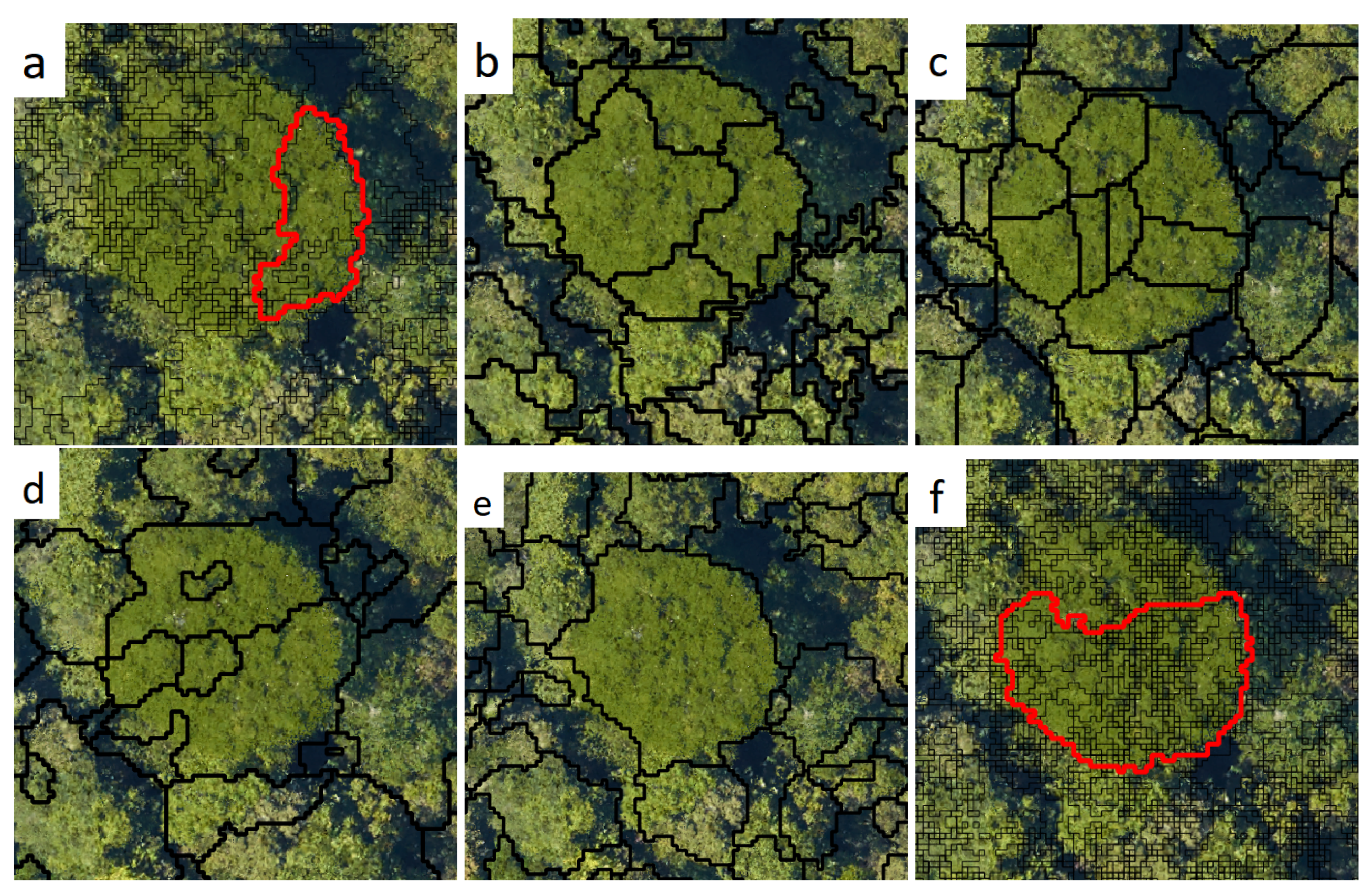
2.1.4. Validation Dataset

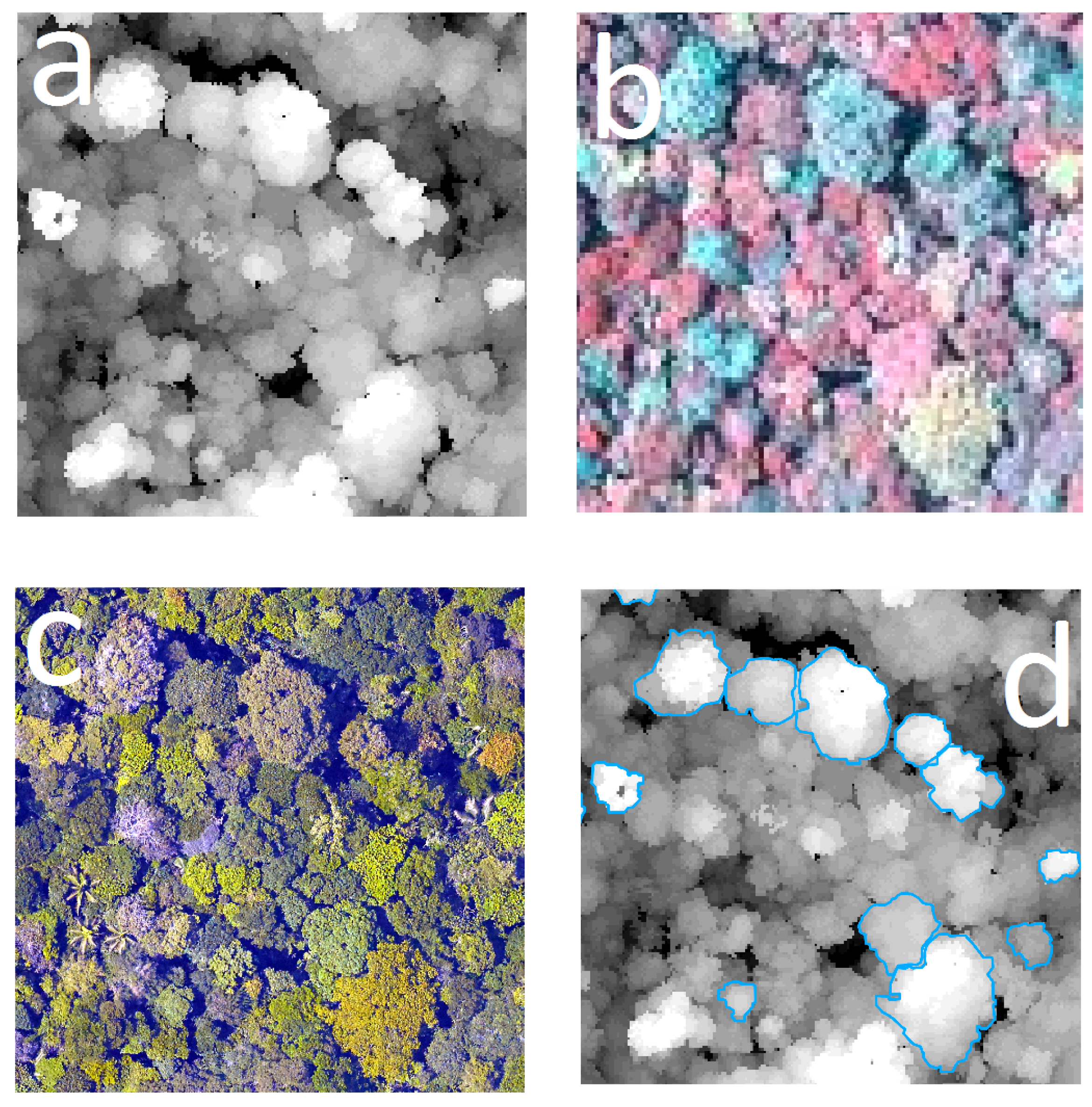
The most clearly visible crowns were manually segmented using colorized ALS points obtained by back-projecting lidar points into the image plane [27]. Manually segmented crowns were then checked in the field, shapes and precise locations of the crowns were corrected when necessary and each crown was associated with a tree from the inventory, leading to a dataset of 1598 manually segmented crowns with a mean crown area of 69 m², used in this analysis as references (Figure 1). The precision of this manual segmentation does not allow to segment smaller subcanopy crowns, and the reference dataset is therefore, biased toward big emergent crowns.

2.2. ITC Delineation Algorithms

Five different algorithms developed by different research teams were compared in this study (

Table 2. ITC delineation algorithms, names used in this paper, quick description of the principles of the algorithm, team developing the algorithm and main publications.

Name	Description	Team	References
AMS3D	Adaptative mean-shift on the point cloud	A.F.	[3,29]
itcSegment	Maxima finding and region growing on the CHM	J.W. & D.A.C.	[4]
Graph-Cut	Graph cut on the point cloud	J.W. & D.A.C.	[30]
Profiler	Maxima finding and watershed on the point cloud	H.H.	[31,32]
SEGMA	Maxima finding and watershed on the CHM	A.P.	[33]

). ALS data from the six plots and one RGB image (only for the plot number 15) were sent to the teams in charge of running the algorithms. Moreover, a reference segmentation was also conducted using both the Canopy Surface Model (derived from the lidar point cloud) and high-resolution RGB-NIR imagery using the e-cognition software [28].

2.2.1. AMS3D

The adaptive mean shift (AMS3D) decomposes a normalized point cloud into 3D clusters that correspond to ITC. It considers the lidar point cloud as a multi-modal 3D distribution where each mode, here defined as a maximum in both height and density, corresponds to the location of a tree crown. The mean shift is used to calculate the modes of the point distribution and to delineate the crowns by clustering the lidar points associated with the corresponding mode [29]. The AMS3D is a non-parametric approach; i.e., it does not assume any predefined model on the crown shape; and relies on a choice of a single biophysical parameter: a multi-scale bandwidth. The latter can be seen as a cylinder the size of which (height and width) can be locally calibrated using tree allometry based on tree height and crown size. A self-calibrated version of the AMS3D has been developed for the regions of the globe where crown size allometry is either nonexistent or it has been derived with high uncertainty (e.g., tropical forests, [3]).

2.2.2. itcSegment

The ITC delineation approach finds local maxima within a rasterized CHM, designates these as tree tops and then uses a decision tree method to grow individual crowns around the local maxima. The approach goes through the following steps: (i) a low-pass filter is applied to the rasterized CHM to smooth the surface and reduce the number of local maxima. (ii) Local maxima are located using a circular moving window; a pixel of the CHM is labelled as local maxima if its value is greater than all other values in the window, provided that it is greater than some minimum height aboveground, where the window size scales with height aboveground based on a regional allometry for crown extent. (iii) Each local maximum is labelled as an ‘initial region’ around which a tree crown can grow. The heights of the four neighbouring pixels are extracted from the CHM and these pixels are added to the region if their vertical distance from the local maximum is less than some user-defined percentage of the local maximum height, and less than some user-defined maximum difference. This procedure is repeated for all the neighbours of cells now included in the region, and so on iteratively until no further pixels are added to the region. (iv) From each region that has been identified, the first-return ALS points are extracted (having first removed low elevation points). (v) A 2D convex hull is applied to these points, and the resulting polygons become the final ITCs. This method has been applied using the R package itcSegment [34]. The itcSegment method has been tested with different allometries, and we selected the allometry producing the better congruence between segmented crowns and the reference dataset in plot number 15.

2.2.3. Graph-Cut

In the Multi-Class Graph Cut (MCGC) approach, a normalized graph cut is applied to the raw 3D point cloud to produce 3D segments corresponding to tree crowns. The point cloud is first converted to a graph by computing similarity weights based on horizontal and vertical distances between points, as well as incorporating ‘prior’ data on tree tops derived from a local window maxima finder. A normalized graph cut is then used to form clusters of well-connected points, which are in turn less-strongly linked to other clusters. The number of clusters is automatically set based upon the structure of the graph and information from the prior tree tops. Candidate clusters are then tested for allometric feasibility based upon a specified height to crown radius relationship (with height computed as aboveground height, based on a model of the ground surface). Feasible clusters are collected for the segmentation, and those clusters that fail the testing have their points rejected and left unassigned. This process is applied in a gridded approach to the full dataset, where sections of the data are sequentially clustered and then the results are merged. A second pass of the MCGC algorithm is then applied to the remaining points that are unassigned, with the goal of finding lower canopy crowns now that the more dominant trees have been segmented. The same process is applied, including allometric testing. After that, the trees from both applications of MCGC are collected and any points left unassigned after the second pass of graph cut are excluded from the list of valid crowns [30].

2.2.4. Profiler

The method initially excludes non-surface and low vegetation (elevation below 3 m) points and smooths the raw elevation values of the rest of the points. It then continues with these steps: (i) locate the global maximum; (ii) generate multiple vertical profiles starting from the global maximum and stretching outwards; (iii) identify the crown boundaries within each profile by detecting between crown gaps and then inspecting the ALS point smoothed elevation values; (iv) cluster all ALS points contained within the convex hull of the boundary points, which were identified within the profiles, as the tallest crown. Clustering the tallest ITC iterates until all ALS points were clustered. Finally, all clustered ITCs that are less than 2 m in crown width are removed as noise. The method was originally developed and tuned for individual tree detection rather than for ITC delineation. In order to improve the resulting ITC delineation, a final stage of marker-controlled watershed segmentation is performed with the clustered crown apexes being the markers. The method is fully automatic and does not require prior assumptions about tree height/width ratio. Between-crown gaps are identified using a statistical outlying mechanism and inspection of ALS elevation values is done using tree height and crown steepness information that is captured on-the-fly from the local ALS data [31,32].

2.2.5. SEGMA: Therefore, Computree Version

This method is based on a detection and filtering of maxima to identify apexes. The crowns are then delimited via a Watershed algorithm and corrected according to geometric criteria. The method is based on the version originally developed in [33], implemented in Computree platform. The maxima filtering step was however, further refined. The steps for detecting maxima are: (i) creation of the DSM (Digital Surface Model) and of the DTM (Digital Terrain Model); (ii) filling of small cavities, (iii) Gaussian smoothing of the DSM, (iv) the detection of maxima. Then the maxima are filtered using a neighbourhood analysis algorithm [Piboule 2016, unpublished], which replaces the filtering by exclusion radius computed from the height of the maxima, used in the original SEGMA method. This algorithm makes a 2D Delaunay triangulation of the detected maxima. On each path connecting two neighbouring maxima, a depth profile is calculated giving, along this path, the vertical distance between the 3D line connecting the two maxima and the DSM. The maximum depth is compared to a threshold provided as a parameter. If it is above the threshold, it is considered that there is a clear separation between the crowns, and both maxima are kept. Otherwise, the maximum with the lowest height is removed. This approach is reproduced iteratively by decreasing height of the detected maxima (altitude of the maxima minus DTM altitude). A minimum radius (no lower maximum is kept if its 2D distance is less than this radius) and a maximum radius (no maximum is eliminated beyond this radius) are also defined to avoid keeping too close maxima or excessive maxima removal. Finally, the detection of the crowns for each apex is performed: (i) a watershed algorithm (flooding of crown initiated from retained maxima) provides a first version of the crown areas. (ii) Geometric criteria (vertical distribution of points, crown circularity and 2D offset between crown mass center and apex position) provides a score that is compared to a threshold to determine whether the crown has a coherent shape or not. If not, the crown is reduced using an OTSU threshold applied to the vertical distribution of the points (detection and suppression of the lowest mode of the distribution). This eliminates any gap part or understory tree that would have been wrongly aggregated in the crown. (iii) After crown reduction, any intra-crown cavities that may have appeared are filled again. The crowns are represented by a raster of crown identifiers, corresponding to the retained apexes (maxima). (iv) This raster can be projected vertically on the vegetation points of the point cloud, in order to obtain a point cloud for each tree.

2.2.6. E-Cognition

This is the only case in which spectral information was used in conjunction with lidar-derived information. RGB data were first projected to the Lab color space, with one channel for Luminance (L) and two color channels (a and b). Canopy gaps (defined as areas with Luminance < 25 or canopy height below 17 m) were masked and a region growing segmentation [35] was then performed. Weighting of the various criteria used for defining heterogeneity in virtual merging decision process were selected by trial and error and set to the following values ( L: 1/a: 1/b: 1, IR: 1 , CHM: 9, scale parameter: 13, shape: 0.2, Compactness: 0.77).

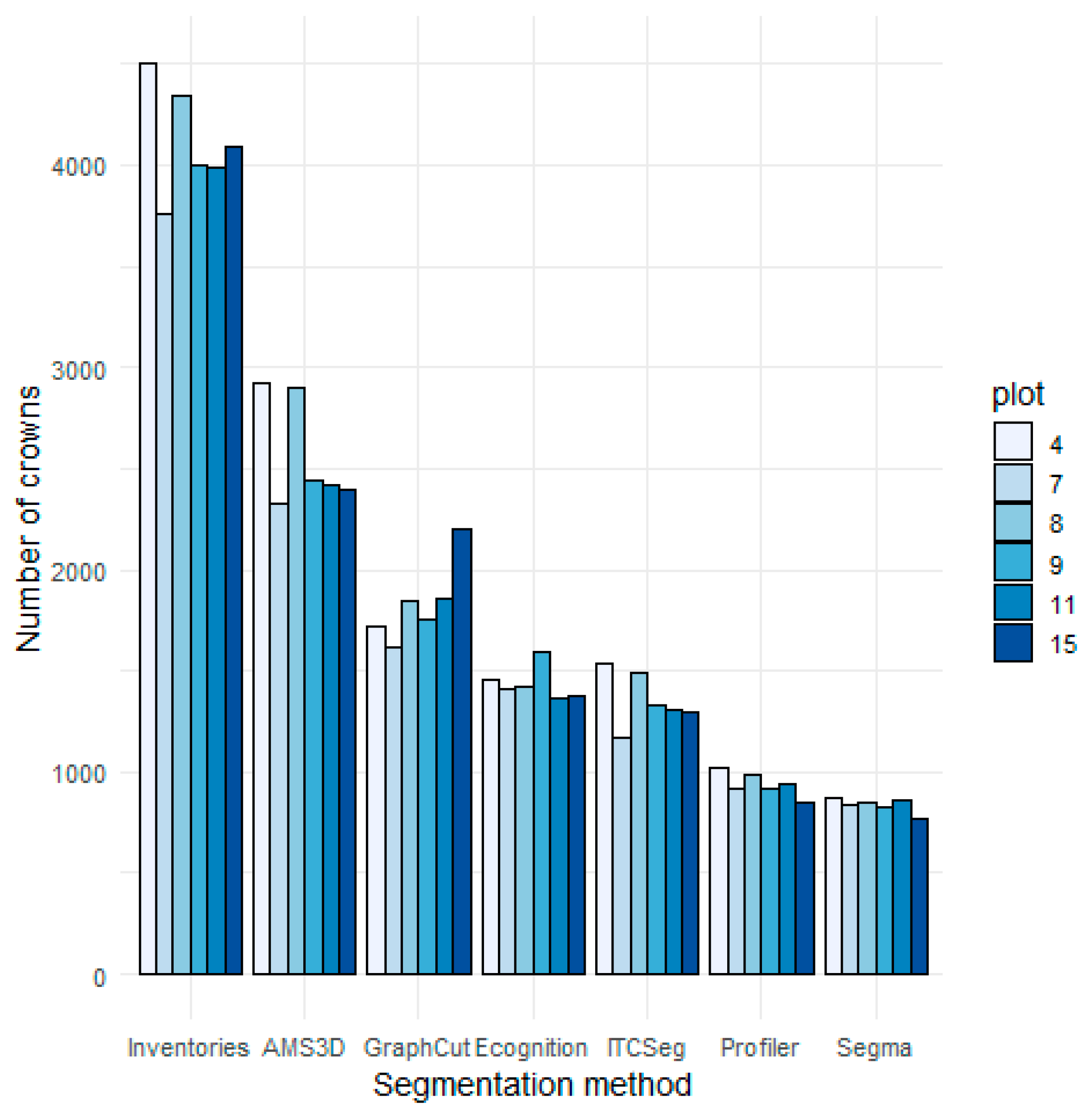
While we could not rigorously compare computing time as the actual segmentation was done on different computing environments we can roughly rank the algorithms in terms of their computing efficiency from high to low in the following order Profiler > SEGMA > itcSegment > AMS3D > Graph-Cut. Without surprise, methods using the CHM are faster than the one considering the entire point cloud. We can also note that computing time tended to increase exponentially with point cloud size for algorithm using the point cloud rather than the CHM.

2.3. Congruence Analysis

The automatic segments were compared with the 1598 crowns manually delineated in the six studied plots of 6.25 ha, hereafter referred to as “reference data”. Each team participating in the study provided a point cloud with each point associated with the ID of a tree. We first rasterized each point cloud (resolution 0.5 × 0.5), keeping the tree ID of the highest point in each pixel. We applied a majority filter (3 × 3 pixels) to reduce the noise and the resulting rasters were converted into polygons. Holes inside crowns were filled and the crowns smaller than 4.5 m² were deleted, 4.5 m² being the area of the smallest manually segmented crown. The resulting polygons were matched against the reference data. Two algorithms used the points cloud and not a surface model (AMS3D and Graph-Cut). These two algorithms can, therefore, segment overlapping crowns and the method described before will trim the crowns that are partially masked from above. Therefore, for these two algorithms, each point cloud segmented as a unique crown was rasterized individually to capture the full extent of the crown. Crowns that are composed of only few points (less than 40 points) or that are too short (<15 m.) are not considered. Moreover, only crowns at least partially visible from the top were considered. Indeed firstly the reference dataset is composed only of dominant or emergent trees (visible from above) and secondly the comparison with the other algorithms for completely masked crowns would not have been possible. For each machine-segmented crown intersecting with a manually delineated crown, the Jaccard Index was calculated. Its value corresponds to the area of the intersection of the two polygons divided by the area of their union (Equation (1)).

$$\mathrm{Jaccard}\mathrm{Index}(A,B)={\displaystyle \frac{|A\cap B|}{|A\cup B|}},$$

(1)

where $\left|A\right|$ and $\left|B\right|$ are the surface areas of the machine-segmented and manually delineated crowns.

A crown was considered correctly segmented if the Jaccard Index was above a threshold value of 0.5. To test the tendency of algorithms to over-segment, another test was conducted. For each reference crown, we detected every automatic crown with more than 50% of their area inside the reference crown. Then they were merged, and the new Jaccard Index was calculated. If it was above the threshold value, the crown was considered over-segmented. A similar test was applied to detect under-segmentation, where the roles of reference and automatic segments were inverted.

2.4. Paired-Trees Analysis

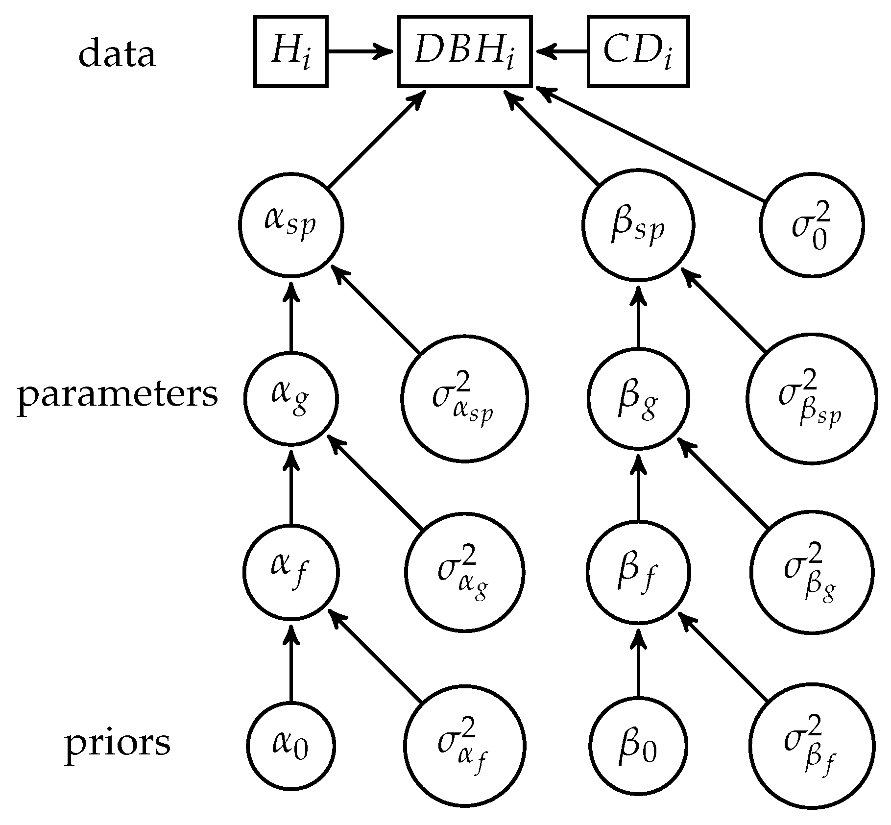
Matching automatic segments with expert segments has limitations since only a subset of the visible crowns are considered in the congruence analysis. Therefore, we used an alternative approach to validate the automatic segmentation which included more of the crowns segmented automatically. First, using data from the manually segmented crowns, we modelled each tree’s DBH (diameter at breast height) using crown area, height, and taxon. Then, we developed an algorithm to optimally pair a crown with a tree from the inventory using the model previously parameterized. Lastly, we used this algorithm on the automatic segments, and checked how well the paired crown/tree fitted the model: if the crowns are better segmented, they should better predict the stem diameter.

The reference data were used to calibrate an allometric model predicting individual trees DBH from the crowns characteristics [2,36,37] (Equation (2)).

$$\begin{array}{c}ln\left(DB{H}_i\right)={\alpha }_{s{p}_i}+{\beta }_{s{p}_i}ln(H_i\times C{D}_i)+\epsilon \\ \epsilon \sim \mathcal{N}(0,{\sigma }_0^2)\end{array}$$

(2)

where $DB{H}_i$ is the diameter at breast height (DBH, in cm) of tree i from species $s{p}_i$, $H_i$ is its height, $C{D}_i$ its crown diameter, and $\epsilon$ the error term. Crown diameter is computed here from irregular polygons as the diameter of a disk of equivalent surface. In our case, tree species identification of the reference data is also available, and can be used to refine this model as allometries can vary among species. To take advantage of the botanical identification of the species, the parameters of the model ($\alpha$ and $\beta$) were modelled as random variables for each species, genus and families, with a hierarchical structure (Figure 2).

$$\begin{array}{c}\hfill {\alpha }_{sp}\sim \mathcal{N}({\alpha }_g,{\sigma }_{{\alpha }_{sp}}^2)\\ \hfill {\beta }_{sp}\sim \mathcal{N}({\beta }_g,{\sigma }_{{\beta }_{sp}}^2)\end{array}$$

(3)

where ${\alpha }_g$ and ${\beta }_g$ are genus-specific parameters sampled from the following normal distribution:

$$\begin{array}{c}\hfill {\alpha }_g\sim \mathcal{N}({\alpha }_f,{\sigma }_{{\alpha }_g}^2)\\ \hfill {\beta }_g\sim \mathcal{N}({\beta }_f,{\sigma }_{{\beta }_g}^2)\end{array}$$

(4)

The family parameters ${\alpha }_f$ and ${\beta }_f$ are sampled in the prior distribution:

$$\begin{array}{c}\hfill {\alpha }_f\sim \mathcal{N}({\alpha }_0,{\sigma }_{{\alpha }_f}^2)\\ \hfill {\beta }_f\sim \mathcal{N}({\beta }_0,{\sigma }_{{\beta }_f}^2)\end{array}$$

(5)

To select the level of taxonomic information to use, we built the same model with different taxonomic information for parameters $\alpha$ and $\beta$: species, genus, or family level, and a model without any taxonomic information (same parameters for all trees). The deviance information criterion (DIC) was then computed for each model to compare them [38]. The model with the most information (species level) had the lowest DIC (

Table 3. DIC for allometric models with different level of taxonomic information.

Level of Taxonomic Information	No Information	Family	Genus	Species
DIC	16,264	15,924	15,573	15,502

).

The allometric model was built and parameters estimated using the package R2jags [39,40].

To pair the segmented crowns with the tree dataset, we took two kinds of information into account. First crown center (computed as the 2D-centroid of crown projection) and trunk location have to be close enough, and second the tree should respect the allometric relation between the crown size and the trunk diameter. We considered those two rules to apply independently, neglecting a possible dependency of crown trunk distance to tree size.

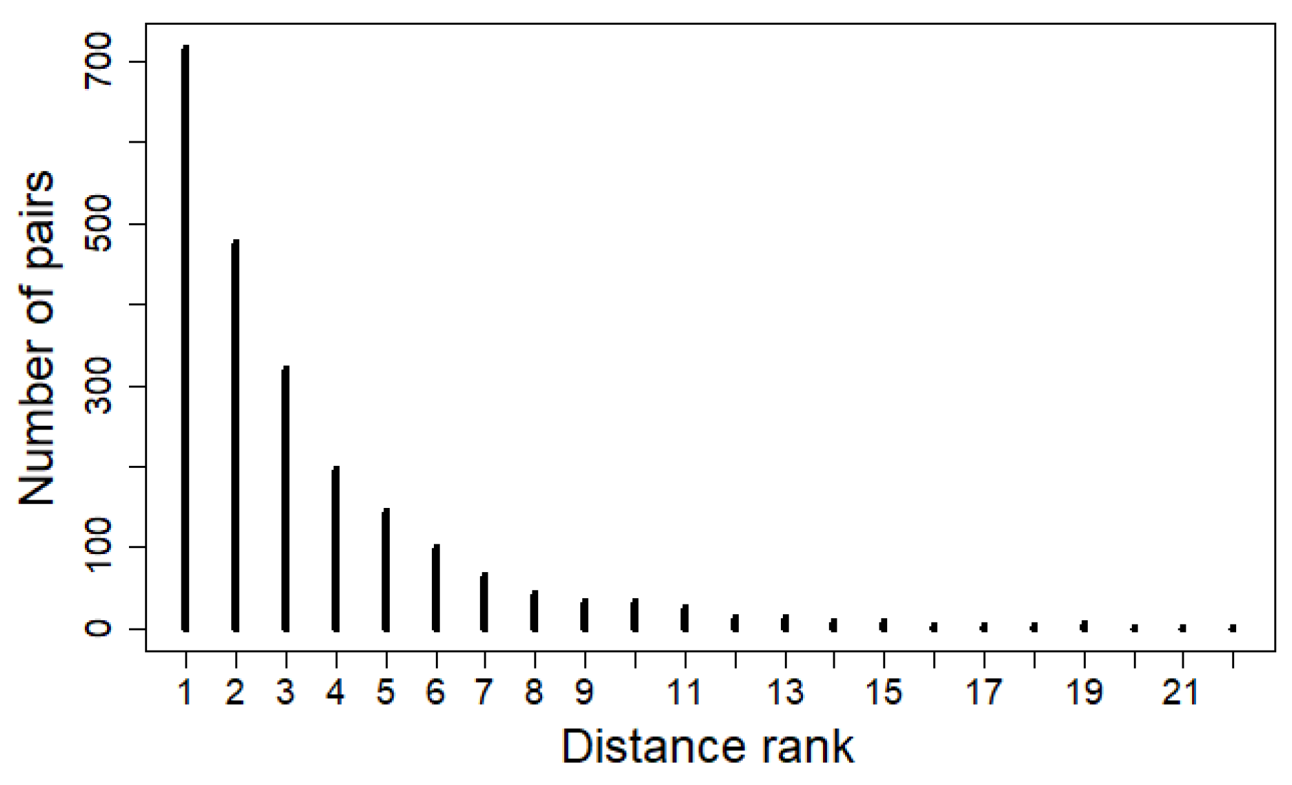
To pair crowns with neighboring trees, we computed the distances between each crown of the reference 1598 crowns and all trunks of the inventory. We then computed the distance ranking of the trunk associated with the crown in the reference data (Figure 3), and fitted an exponential distribution on the ranks:

$$d_{i,j}=\alpha e^{-\alpha ·r_{i,j}}$$

(6)

where $r_{i,j}$ is the rank of the tree j associated with the crown i, and $\alpha$ the parameter of the exponential distribution.

We used the rank and not directly the distance between the crown and the associated tree because most crown centroids are at least few meters away from the closest neighboring tree and therefore, the probability of being extremely close (less than two meters) is actually very small. Using the distance distribution would have penalized pairs with trunk and crown very close to each other.

Then the pairing algorithm pairs each crown with the tree with the highest $p_{i,j}$.

$$p_{i,j}=d_{i,j}\times g_{i,j}$$

(7)

where $g_{i,j}$ is the density function of the normal distribution corresponding to the likelihood of the allometric model (Equation (2)):

$$\begin{array}{c}{g}_{i,j}={\displaystyle \frac{1}{{\sigma }_0\sqrt{2\pi }}}{e}^{-{\displaystyle \frac{1}{2}}\left({\displaystyle \frac{ln\left(DB{H}_j\right)-\widehat{ln\left(DB{H}_i\right)}}{{\sigma }_0}}\right)}\\ \widehat{ln\left(DB{H}_i\right)}={\alpha }_{s{p}_i}+{\beta }_{s{p}_i}ln(H_i\times C{D}_i)\end{array}$$

(8)

The maximization of this likelihood avoids attributing stems to crowns of disproportionate size.

Finally two crowns could be paired with the same stem if we just maximized the density $p_{i,j}$. therefore, stems are ordered by decreasing DBH, and they are paired one after another in that order, with the segmented crown having the largest $p_{i,j}$ in the neighborhood of the stem (15 m). When a crown is allocated to a stem, it is no longer available for others.

To have an estimation of the pairing confidence, the difference ${\Delta }_p$ between $p_{i,j}$ of the associated tree and the second largest $p_{i,j}$ is computed for each crown.

The allometric model was then used to evaluate the different segmentation algorithms. The predicted DBH were compared with the DBH from the associated trees using the RMSE. As different segmentation methods might segment different number of crowns, the RMSE was computed for bins of 100 pairs of increasing DBH to know how well the different algorithm segment crowns from different sizes. Moreover, the RMSE was also computed using only crowns and trees that were matched with a ${\Delta }_p$ in the 40% highest ${\Delta }_p$ of the pairs for the 5000 largest stems. Additionally, the RMSE was also computed for the trees that belonged to the reference dataset. The pairing algorithm and validation were realized using the packages raster, rgdal and rgeos on R [40,41,42,43].

3. Results

3.1. Segmentation Results

The different algorithms produced highly different numbers of segmented crowns (

Table 4. Results for the six segmentation algorithms.

Algorithm	Mean Number of Crowns per Plot	Mean Area of a Crown (m2)	Area of Plots Segmented	% of Crowns Segmented Paired with a Stem
AMS3D	2564	32.46	91%	37%
SEGMA	837	53.12	65%	87%
E-cognition	1435	40.40	86%	61%
Graph-Cut	1832	34.38	66%	82%
itcSegment	1353	43.86	88%	86%
Profiler	936	71.17	97%	88%

and Figure A1), from 837 crowns per plot for SEGMA to 2564 for AMS3D. An example of segmentation can be found in the Appendix B, Figure A2. To avoid border effects, crowns that were closer than one meter from the border of the plots were removed from the results. Mean crown areas vary from 32.46 m² for AMS3D to 71.17 m² for Profiler. Algorithms segmenting more crowns tended to also segment smaller crowns (Table 4 and Figure 4). Higher crowns were larger for all segmentation methods, but the relationship between crown area and height was clearer for some methods (AMS3D, itcSegment, Profiler and SEGMA) than others (Graph-Cut and E-cognition, Figure 5). Some methods used an allometric relationship between crown diameter and height. This was the case for the Graph-Cut method, which re-segmented crowns if their diameter is too large. It was also the case or for the itcSegment method through a variable window size, and for AMS3D through the variable bandwidth.

3.2. Congruence Analysis

Almost 74% of the crowns segmented by the AMS3D were associated with a crown from the reference with a Jaccard index $\ge 50\%$. This was the only method clearly outperforming E-cognition’s multi-resolution segmentation, which used additional spectral information. Algorithms with more matching crowns also tended to have a better mean congruence level between the manual and automatic crown (higher Jaccard index) (

Table 5. Results of the congruence analysis for the six segmentation algorithms.

Algorithm	Crowns with a Match (Jaccard Index $\ge 50\%$)	Mean Jaccard Index	Crowns with a Match, Under-Segmentation	Crowns with a Match, Over-Segmentation
AMS3D	73.8%	71.4%	76.0%	93.7%
E-cognition	59.1%	67.1%	63.6 %	74.0%
SEGMA	55.4%	67.5%	68.4%	61.4%
Graph-Cut	54.3%	69.1%	56.3%	71.0%
itcSegment	43.8%	64.9%	46.8%	67.3%
Profiler	30.5%	60.3%	38.1%	39.4%

).

Most algorithms seem to have a greater tendency to over-segment than under-segment, except for the Profiler method which seems fairly balanced, and the SEGMA method which tends to under-segment crowns (Table 5 and Figure A2).

3.3. Paired Tree Validation

When applied to the reference dataset, the pairing algorithm paired 76% of the crowns with the right stems. For the remaining 24%, the algorithm tended to attribute stems with a smaller DBH than the reference stem DBH (Figure 6).

The pairing algorithm was then applied to the segmented crowns to attribute trees from the field inventories to each crown. Then the allometric model was applied to the resulting pairs (Equation (2)). The RMSE was computed for the 5000 biggest trees to make the comparison between algorithms possible. The lowest RMSE was obtained with the Graph-Cut segmentation (7.64), followed by AMS3D, itcSegment, SEGMA, Profiler, E-cognition (

Table 6. Results (RMSE) of the allometric model applied to dendrological field data and crowns segmented by the different algorithms. For the two first lines, the RMSE was computed for the 5000 largest stems which were automatically paired with a segmented crown, and for the last line RMSE ref was computed with the pairs that are part of the reference dataset (the proportion of the reference dataset crowns that are segmented is added in parenthesis).

	AMS3D	SEGMA	Graph-Cut	itcSegment	E-Cognition	Profiler
RMSE	7.67	9.02	7.64	7.75	10.91	9.47
RMSE 40%	3.58	4.70	3.58	3.97	5.33	4.24
RMSE ref	8.92 (63%)	8.86 (60%)	9.33 (67%)	8.67 (63%)	12.92 (42%)	8.41 (62%)

) in that order. All methods had lower RMSE when considering only the 40% with the highest pairing confidence, and results for all pairs or considering only the 40% with the highest pairing confidence were roughly consistent among methods. In particular, the two best performing methods remained AMS3D and Graph-Cut.

The RMSE was overall larger for small DBH, but also for very large DBH. The AMS3D and Graph-Cut methods clearly outperformed other methods from stems below 40 cm DBH, and AMS3D outperformed all other methods from stems below 30 cm DBH, confirming that 3D methods take advantage of the 3D structure of the lidar point cloud to segment crowns that are only partly visible from above (Figure 7). On the other hand, the SEGMA and Profiler methods had the lowest RMSE for the largest trees (DBH > 60 cm). Overall, the methods that are good at segmenting crowns paired with big trees tend to have reduced accuracy when segmenting crowns paired with small trees, and vice versa. The methods having the most crowns paired with trees also tend to have high RMSE for the smaller crowns (number of trees > 7000 for E-cognition, itcSegment and Graph-Cut on the right in Figure 7). There is indeed a trade-off between the number of crowns actually paired with stems from the inventories and the quality of the pairing evaluated with the RMSE (see Table 4).

4. Discussion

This study focuses on the application of ITC delineation methods in a tropical, dense and diverse forest. Our results confirm that different segmentation methods lead to highly different results, and that the use of the entire 3D point cloud, instead of the CHM derived from this point cloud, is clearly beneficial in dense forests (Figure A2 and Figure A3). The performance of CHM-based methods is usually much better in coniferous forests than in deciduous or mixed forest stands [9,13,14,21,44], and 3D methods have shown better results in “flat crowns” forests [45] that are common in windswept regions or during secondary succession.

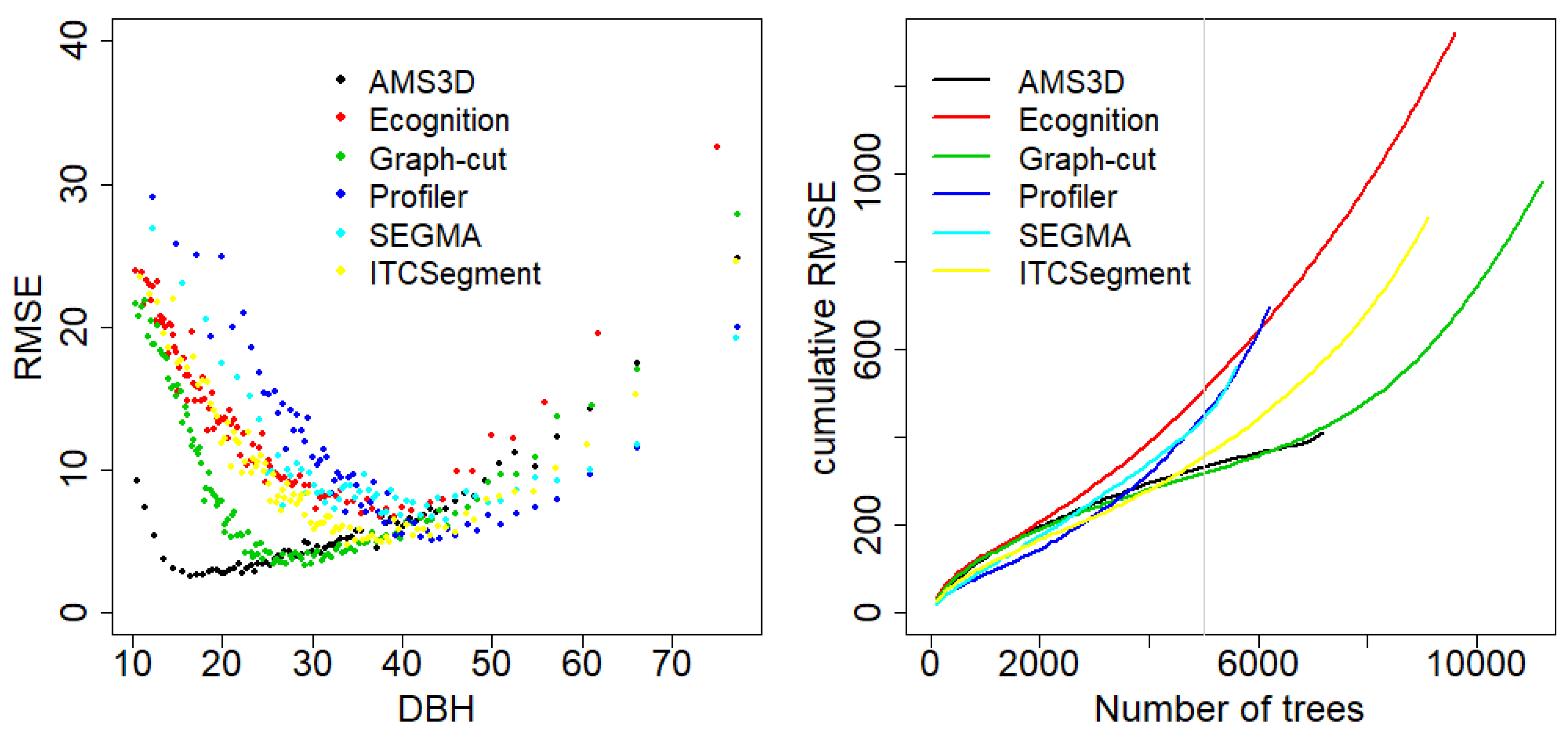
Our benchmark identified the AMS3D method developed in [3,29] as the best method to segment crowns, it clearly has the highest number of crowns with a match, but also the highest mean Jaccard index when comparing the segmented crowns with the reference dataset (Table 5). The difference is less clear when all segmented crowns are taken into account and paired with inventoried trees (Table 6 and Figure 7). Indeed, even though the AMS3D method performs clearly better at segmenting relatively small crowns (associated with stems around 20 cm DBH), the Graph-Cut method also performs well for intermediate small crowns (associated with stems around 30 cm DBH), while the methods Profiler and SEGMA better segment larger crowns (associated with stems between 40 and 60 cm DBH for Profiler, and around 80 cm for SEGMA). Overall, all methods perform better for intermediate sizes than for very small or big crowns (U-shaped pattern of the Figure 7 on the left), and the two methods using the 3D structure of the point cloud perform better than the others for relatively small crowns. 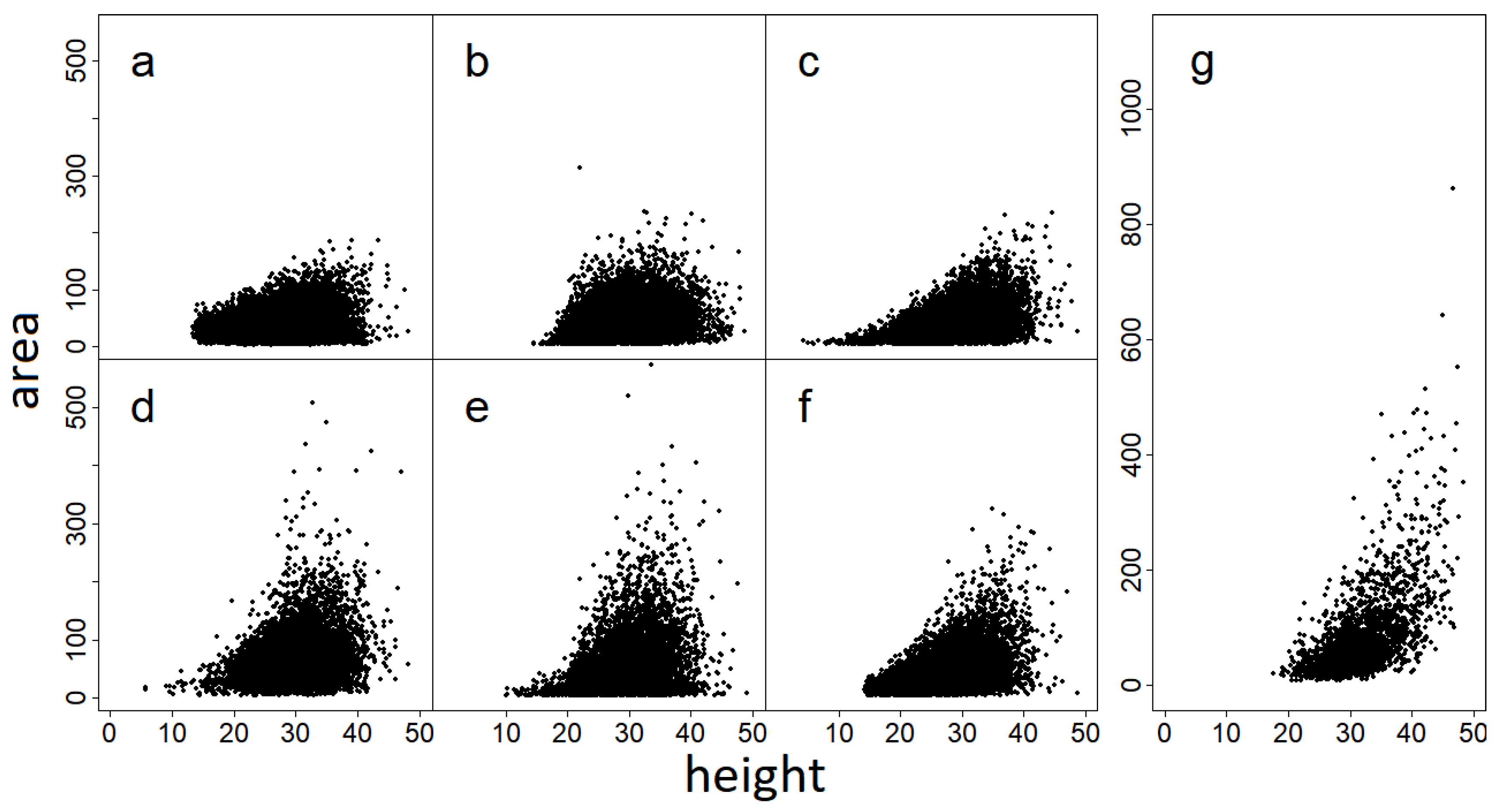These differences can also be related to the size of the crowns segmented (Figure 5); Profiler and SEGMA are the only methods segmenting some very large crowns (area > 300 m²), and are also the one over-segmenting the less (Table 5). On the other hand, even though the AMS3D method is the only one segmenting small crowns, it tends to over-segment a lot. AMS3D is also the only method in this benchmark using the normalized point cloud. Normalizing the point’s heights does not change the point clouds geometry too much in the forest of Paracou because the terrain is even, without steep slopes. But this could clearly affect results in hilly or mountainous forests [9].

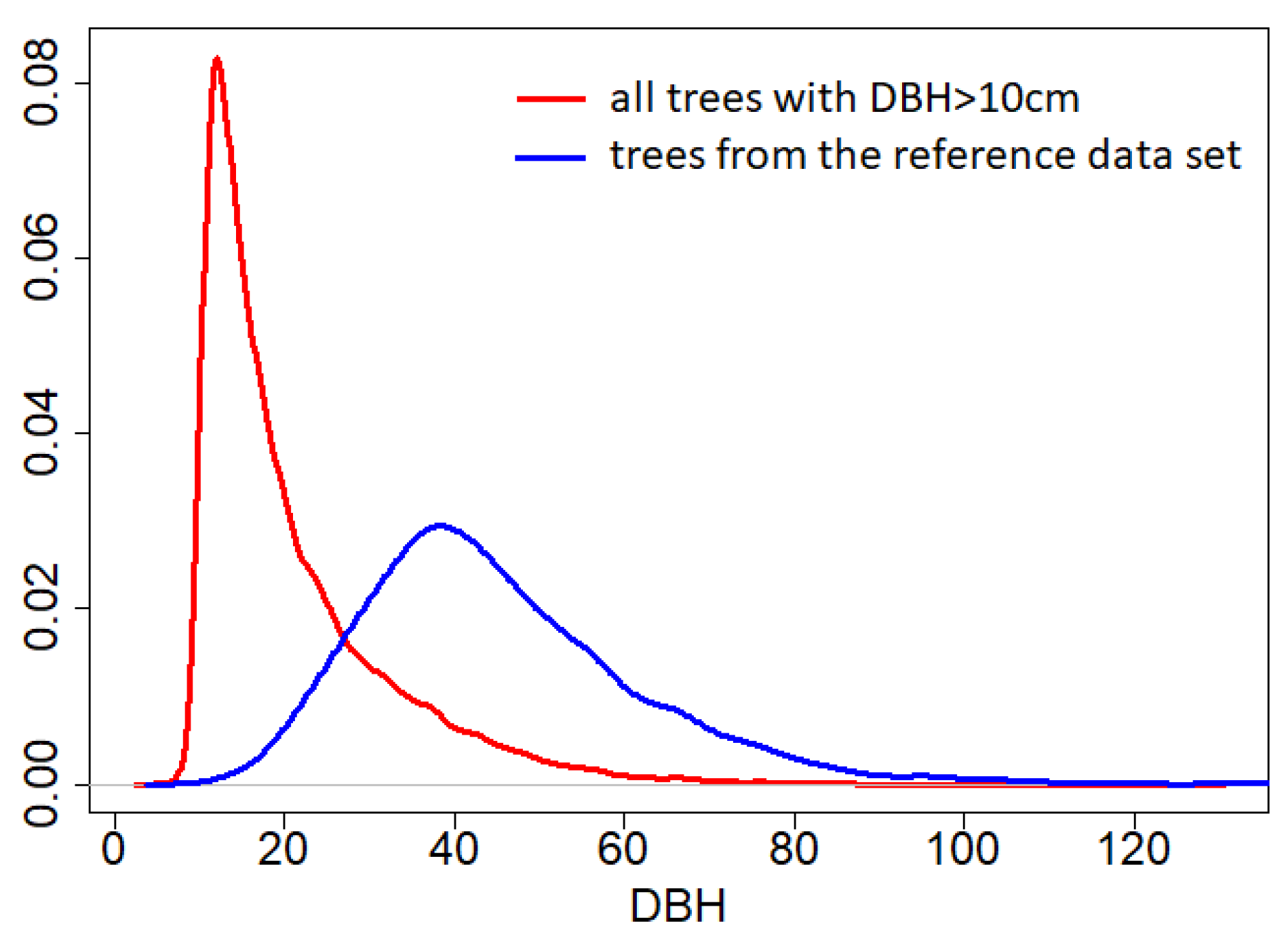
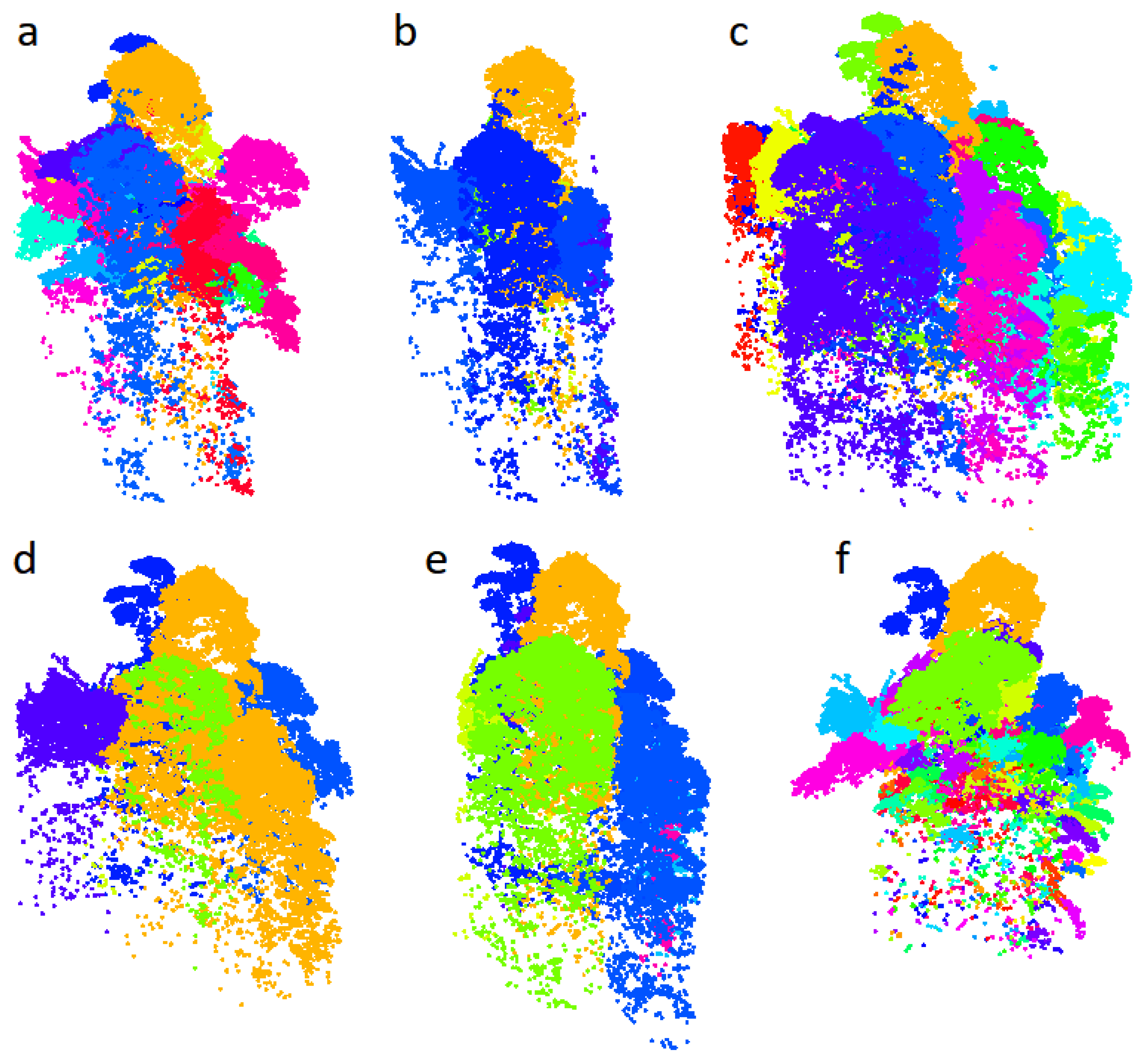
Moreover, differences of performances are based on the projected crowns, and on the comparison with a reference dataset that contains mostly tall canopy trees, the manually segmented crowns being preferably selected among the largest since they need to be clearly visible from above to be segmented (Figure 8). The data presented is not adapted to evaluate the efficiency of the algorithms to detect subcanopy trees, despite the highly different understory segmentation produced by the different algorithms (Figure 9).

This is also why most methods appear to over-segment crowns. Reference crowns tend to be spaced out while the automatic crowns are often adjacent. Therefore, it is more likely to have several automatic crowns in a manual one than the opposite. This limitation also prevents a complete omission and commission study, often conducted in this kind of benchmark [22,23,47]. Instead of a study of commission and omission rates on all the segmented crowns, we proposed an estimation of the fit of the DBH predicted by the segmented crowns area to the DBH measured during the inventories [2]. This estimation relies on the pairing method, which is slightly biased toward small trees (Figure 6). 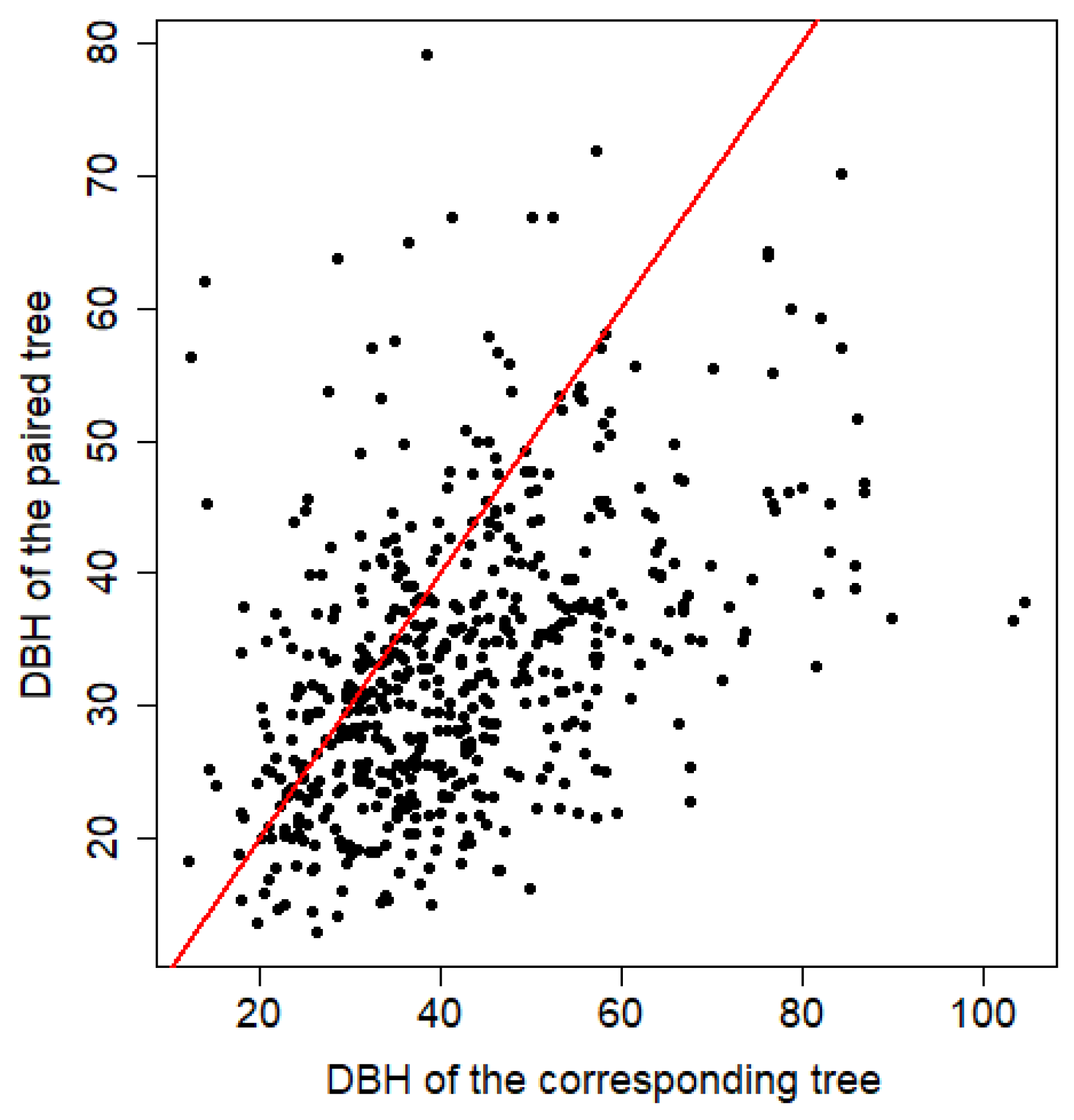Indeed, crowns are often paired with trees of smaller DBH than the reference tree validated in the field, but reference trees are tall and large, which may explain this bias (Figure 8). Moreover, we made the assumption of independence between the trunk-crown distance and the tree DBH, but large trunks are potentially further from their crown centroid than small trees. Again, our reference dataset does not allow a complete study of this relation because it predominantly includes fairly large dominant trees.

The limitations of our benchmarking approach largely stem from the multi-layered structure of the tropical forest: small trees are difficult to see in the airborne imagery and therefore, can hardly be included in the reference dataset. In addition, the point density in the understory is probably too low to achieve a good description of individual crowns below the upper canopy even using high density point clouds as was available for this study (for instance, the point density decreases to less than 5 points/m² if we consider only points that are lower than 10 m from the ground in plot number 4). Point density varies from one plot of the study to another (Table 1), without clear effect on the segmentation results. An evaluation of the effectiveness of subcanopy trees segmentation could however, be attempted by using TLS data as reference [48]. However, different tree segmentation methods from TLS point cloud exist and have not all been applied and tested on tropical forest data.

The different performances of the methods tested in this benchmark should raise awareness of the use of an appropriate segmentation method depending on the segmentation aim. Especially, the method considered may vary if the segmentation focuses on big emergent crowns or smaller subdominant crowns. The main purpose of remote tree mapping in tropical forests remains often to estimate aboveground biomass (AGB) and map carbon. Most of the biomass in tropical forests is stored in big trees [49], thus, we might want to segment big crowns precisely. Further improvement in segmentation of these dominant and emergent crowns may be expected if relevant spectral information can be taken into account (be it hyperspectral or multispectral data, airborne or space borne). Lidar reflectance information can also be used as successfully shown in [50] who used multispectral lidar. However, by including crown diameter in the equation predicting AGB, the error due to over-segmentation of big crowns is reduced [2,36]. The bias induced by the wrong detection of smaller subcanopy trees may therefore, be the most important error to correct to accurately measure AGB. To this end, segmentation methods based on the point cloud are promising, AMS3D method showing good results in tropical forests [3,29]. An improvement of these methods can arise from the use of ALS acquired by UAVs, producing very high point cloud densities [51] and allowing to better characterize the subcanopy layers.

This study confirms the specificity of tropical forests and the need for specific segmentation methods calibrated for this kind of forests [3]. For instance, the method developed in [52] to detect trunks in eucalyptus forests from Australia relies precisely on the ability of the ALS data to detect trunks, and is not widely transferable to other forests in particular closed canopy forests. More flexible methods, like those used in this benchmark, are more generic but also benefit from local allometric relations between crown size and tree height to improve fit.

Our results confirm that the methods based on the 3D point clouds are effective to find and segment crowns in dense tropical forests, especially the mean shift algorithm [3,29]. Moreover, it is fairly straightforward to adapt to point clouds enriched with spectral information, allowing a better identification and segmentation of tree crowns [50].

5. Conclusions

In the present benchmark study, the mean-shift 3D method outperformed the other methods tested for the congruency analysis (congruence with 1498 crowns manually delineated on high-resolution imagery), and the two methods based on the 3D point cloud (AMS3D and Graph-Cut) performed the best for the pairing validation (plot level consistency in automatic crown-stem mapping of 5000 largest stems). This indicates that crown segmentation in a multi-layered closed canopy forest can be better improved by using 3D segmentation methods rather than relying mostly on the canopy surface model. Future improvement of current methods may stem from the fusion of lidar and spectral information [53,54]. Due to increasing occlusion levels towards the ground, segmentation of subcanopy trees in tall dense forests remains an open challenge. Very high density close range UAV lidar may help alleviate the problem to some extent. However, even if individual tree segmentation will be limited to the dominant or subdominant trees, crown size distribution provides new insights on tree structure and improved carbon mapping opportunities which may be less dependent on local calibration than current area-based models [2,55].