Integrated Use of Satellite Remote Sensing, Artificial Neural Networks, Field Spectroscopy, and GIS in Estimating Crucial Soil Parameters in Terms of Soil Erosion

Abstract

Soil erosion is one of the main causes of soil degradation among others (salinization, compaction, reduction of organic matter, and non-point source pollution) and is a serious threat in the Mediterranean region. A number of soil properties, such as soil organic matter (SOM), soil structure, particle size, permeability, and Calcium Carbonate equivalent (CaCO₃), can be the key properties for the evaluation of soil erosion. In this work, several innovative methods (satellite remote sensing, field spectroscopy, soil chemical analysis, and GIS) were investigated for their potential in monitoring SOM, CaCO_3, and soil erodibility (K-factor) of the Akrotiri cape in Crete, Greece. Laboratory analysis and soil spectral reflectance in the VIS-NIR (using either Landsat 8, Sentinel-2, or field spectroscopy data) range combined with machine learning and geostatistics permitted the spatial mapping of SOM, CaCO₃, and K-factor. Synergistic use of geospatial modeling based on the aforementioned soil properties and the Revised Universal Soil Loss Equation (RUSLE) erosion assessment model enabled the estimation of soil loss risk. Finally, ordinary least square regression (OLSR) and geographical weighted regression (GWR) methodologies were employed in order to assess the potential contribution of different approaches in estimating soil erosion rates. The derived maps captured successfully the SOM, the CaCO₃, and the K-factor spatial distribution in the GIS environment. The results may contribute to the design of erosion best management measures and wise land use planning in the study region.

1. Introduction

Soil erosion is a complex four-stage dynamic process involving soil detachment, breakdown, transport, and subsequent deposition of sediments [1]. Erosion is a naturally occurring process that affects all landforms by wearing away a field’s topsoil by the physical forces of water and wind or through forces associated with farming activities such as tillage. Soil erosion can be either a gradual process, continuing relatively unnoticed, or it may occur at an alarming rate, causing serious loss of topsoil, which is high in organic matter [2]. Soil erosion removes organic matter and important nutrients and prevents vegetation growth, which negatively affects overall biodiversity. The specific phenomenon is denoted as the biggest threat to soil fertility and productivity. It changes the physical, chemical, and biological characteristics of soil, leads to a drop in potential agricultural productivity, and gives rise to concerns about food security, especially in the context of a growing world population [3]. Soil erosion may pose a threat to food security if we consider that about nine billion people should be fed by 2050 [4]. Therefore, global agriculture production has to be intensified, presumably on a reduced proportion of land as soil erosion, soil sealing, and salinization increasingly take their toll on the landscape [4]. Nevertheless, the effects of soil erosion go beyond the loss of fertile land, since it can also lead to increased pollution and sedimentation in streams and rivers, closing the waterways and causing declines in fish and other marine species. Degraded lands have also reduced capacity to hold onto water, sometimes causing intensification of flooding.

Mediterranean Europe is a world hotspot extremely prone to erosion, as it suffers from long dry periods followed by heavy erosive rainfall on steep slopes with fragile soils, resulting in considerable amounts of erosion [5]. It is a fact that several Mediterranean spots have already reached a stage of irreversibility in terms of soil erosion, while in some places, there is little soil left [6]. Greece is one of the most erosive areas of the Mediterranean countries [4], and therefore, it is necessary to estimate soil erodibility and identify areas of high or low soil erosion risk. Specifically in Crete (Greece), research studies have already monitored and estimated the soil erosion process in several basins [6]. The study in [7] quantified the soil loss amount in Chania, Crete, and depicted the watersheds that are exposed to greater soil erosion risk in the study area. [8] investigated soil erosion in southern central Crete, Greece, in the Asterousia range, where soil erosion is already widespread [9], and the region appears desertified.

Different approaches have been employed in the relevant scientific literature regarding the soil erosion research. Either integrated or individual employment of innovative techniques such as satellite remote sensing, geostatistics, geomorphology, field spectroscopy, machine learning, and combined in situ and laboratory soil reflectance measurements are considered to be promising approaches to estimate various soil properties [10]. Geostatistics, including interpolation and spatial linear regression methods, have been used by several researchers in order to monitor soil organic matter (SOM), CaCO₃, and soil erodibility (K-factor) [11,12,13]. Laboratory analysis is sometimes proven inadequate when trying to investigate the soil erosion regime, especially in wider areas. In such cases, a big number of well spatially distributed samples should be collected for further analysis, which usually turns out to be an expensive and time consuming process. Therefore, the combination of laboratory analysis with geostatistics and remote sensing may be ideal to enable the environmental change monitoring in terms of cost and time. Earth observation (EO) satellites in particular have proven very beneficial in upscaling local field studies to relatively large areas [14,15,16,17]. Satellite remote sensing is virtually the only data source that permits a repeated monitoring of land degradation dynamics [18]. In this context, both [10] and [13] applied integrated use of geostatistics, geoinformatics, and field spectroscopy to study the correlation between soil erosion and various soil parameters such as SOM, CaCO₃, and K-factor.

Initially, the most common field scale model for the estimation of soil erodibility risk was the Universal Soil Loss Equation (USLE) [19], which was later revised to the Revised Universal Soil Loss Equation (RUSLE) [20]. Both USLE and RUSLE equations are empirical models whose parameters contain uncertainty [21]. Reference [22] noted that nowadays, the RUSLE model is a widely used method in the Mediterranean for the estimation of soil erodibility risk and the assessment of soil erosion effects. Furthermore, numerous scientists have already employed the integrated use of satellite remote sensing data, the GIS approach, and the RUSLE methodology in monitoring and estimating soil erosion rates [23,24,25,26]. Following that, machine learning approaches such as artificial neural networks (ANN) have been successfully used in the recent past to simulate soil erosion processes [27,28,29]. In those cases, ANNs have been utilized to describe the nonlinear relationships between eroded soils and relevant soil parameters such as SOM and CaCO₃. Continuously, the accurate spatial identification of SOM and CaCO₃ permits the subsequent identification of K-factor. K-factor is an estimate of the ability of soils to resist erosion based on the physical characteristics of each soil.

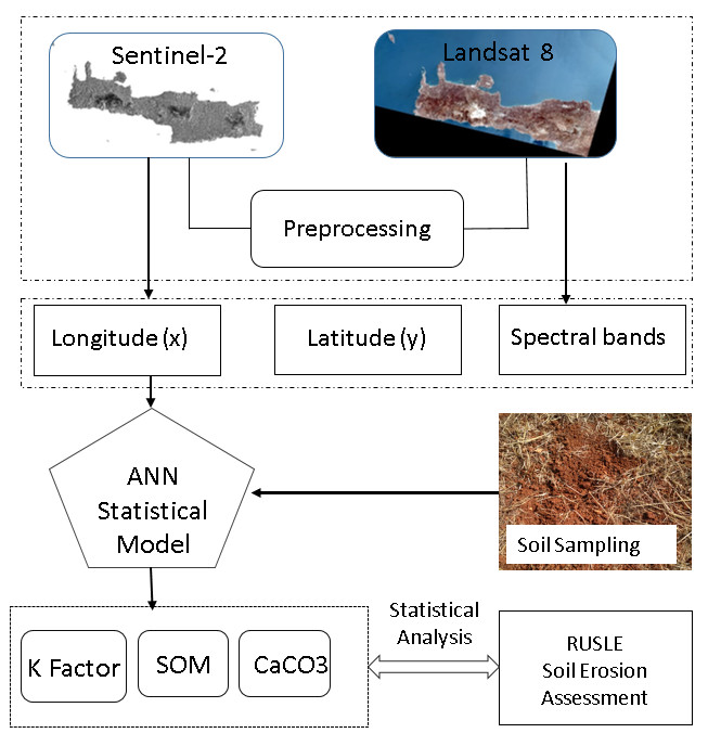
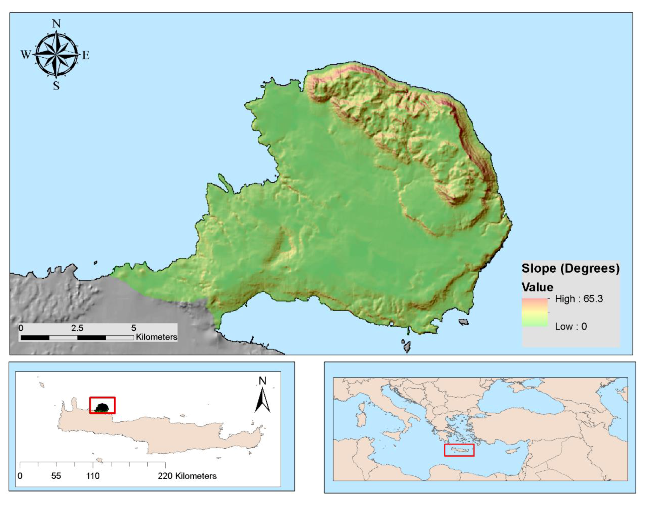
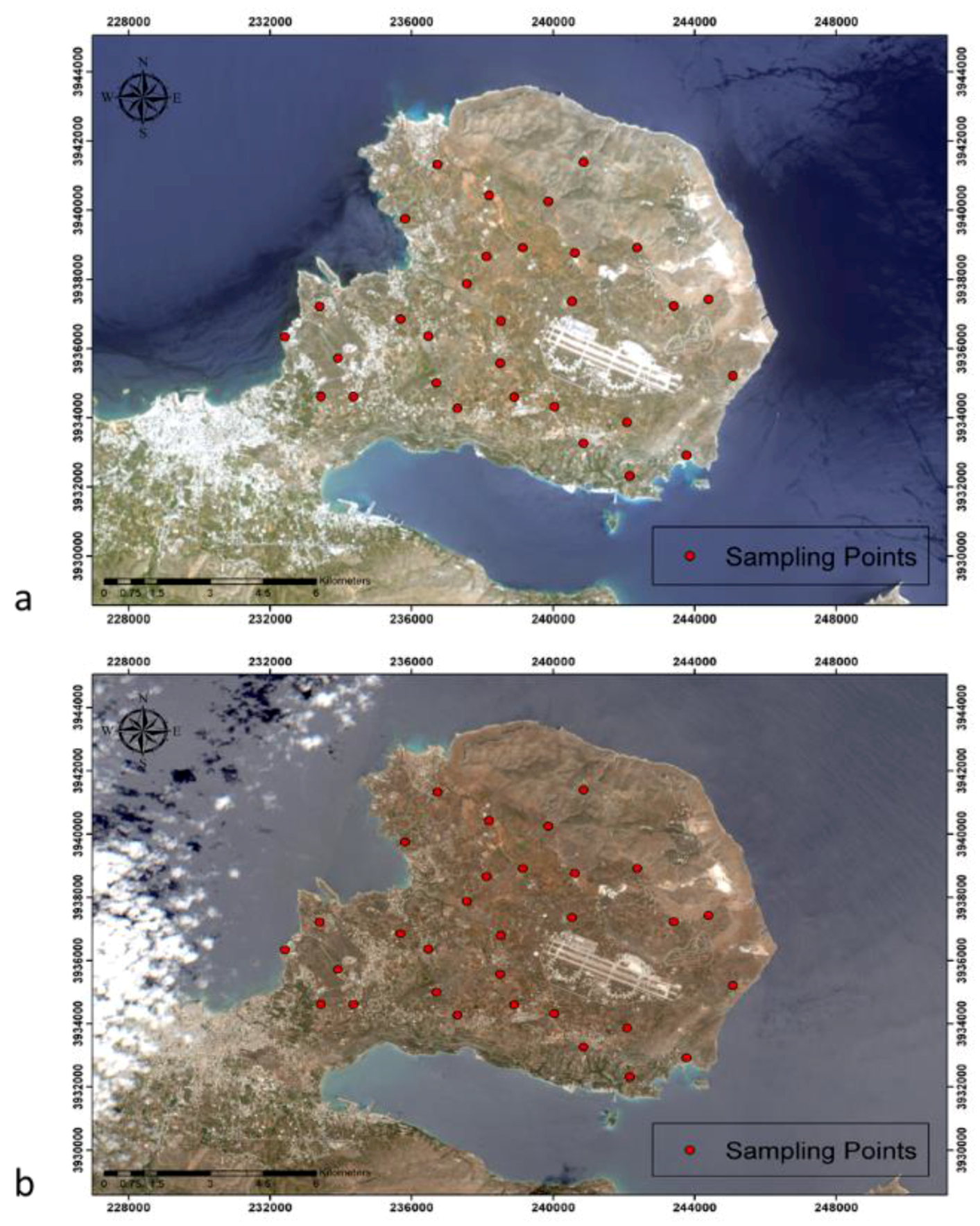
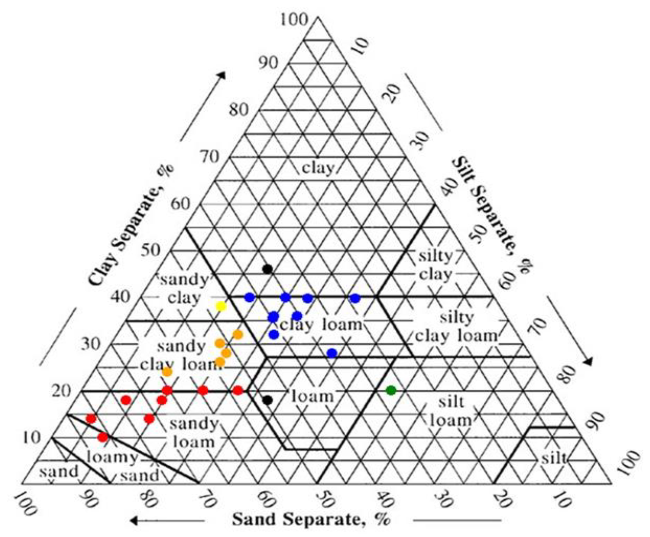
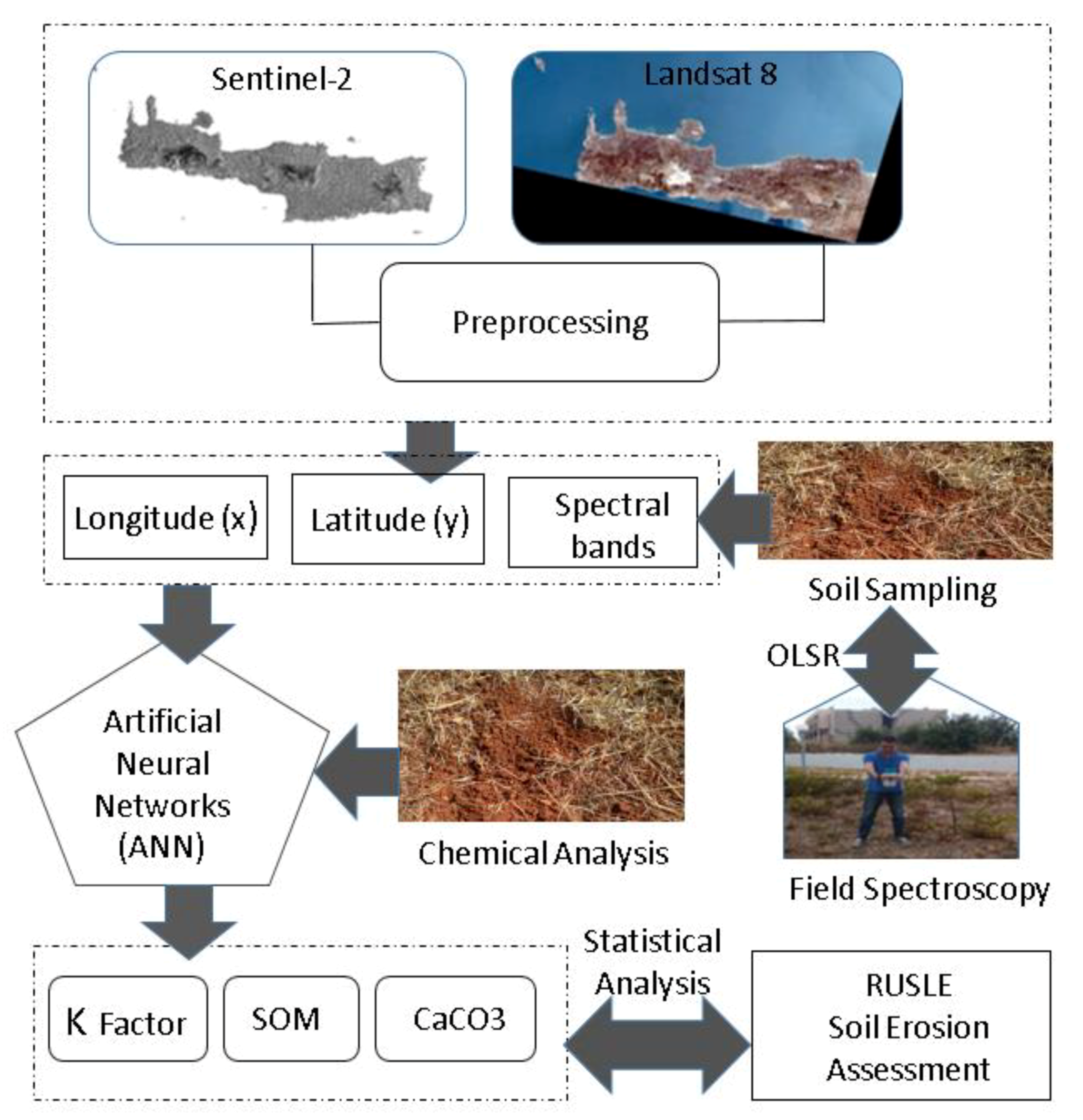
In this study, the soil erosion phenomenon is extensively investigated in the Akrotiri cape in Chania, Crete. At first, laboratory analysis of 30 soil samples in terms of texture and chemical composition collected from corresponding study spots was conducted. Continuously, EO data (Sentinel-2, Landsat 8) combined with machine learning approaches (ANNs) derived SOM and CaCO₃ maps of the study area in the GIS environment. The aforementioned maps were used for the estimation of K-factor, which expresses the susceptibility of soil to erode [30]. The results of the machine learning developed maps were compared with respective maps developed from geostatistics (spline method) analysis in terms of accuracy. In addition, the RUSLE model was also applied in the study area, and the soil loss outputs were cross-compared with the already estimated soil parameters (SOM, CaCO₃). Finally, soil samples spectral data as derived from field spectroscopy campaigns were used in order to assess and correlate soil properties with specific spectral bands.

2. Study Area and Data

2.1. Study Area

The study area was the Akrotiri cape located in the northeastern part of Chania city in Crete (Figure 1), covering an area of approximately 112.6 km². The Akrotiri cape offers great diversity on the topographic relief, being both characterized as rocky and lowland area, whereas it includes a coastal zone of approximately 59.55 km with steep shores. The elevation ranges from 0 to 529 m (Skloka peak in the eastern part of the region). The rocky zone is located in the northeastern part of the Akrotiri region, where the elevation ranges approximately between 350-420 m. The area consists mainly of limestone rocks, which produce carbonate karst formations such as gorges, streams, sinkholes, and caves. Flat relief with a maximum altitude of approximately 220 m characterizes the lowland zone of the Akrotiri cape. In the north-northeast part, the hilly area is sinking into the Cretan Sea, shaping the rocky coasts with steep slopes.

The climate in the study area is characterized as temperate Mediterranean and particularly dry-hot. Sunshine covers 70% of the days of the year. Summers are warm and dry, while winters are relatively mild [31]. The average annual precipitation for the broader area of Chania is estimated at about 665 mm [6] and takes place mainly from November to March. Predominant land-uses are forests and semi natural areas (47.2%), where sclerophyllous vegetation and shrubs predominate, suitable for pasture. In addition, heterogeneous agricultural areas (27%) and agricultural areas (18.7%) also prevail. In the central and the central-western area of the Akrotiri cape, there is intensive anthropogenic activity, i.e., road networks, commercial activities, and residential areas. Furthermore, the soil in the study area has high permeability, resulting in high infiltration rates and good drainage. The soil is not continuous, as the rocky part occupies 50-70% of its surface. Based on field observations and monitoring, sheet, rill, and gully erosion caused by running water are predominant at the study site.

2.2. Satellite Imageries

For the study needs, two different satellite images from two different sensors, namely Sentinel-2 and Landsat 8, were acquired and incorporated in the overall research (Figure 2).

The two images cover the study area (Akrotiri Cape) during the study period (July 2018). The specifications of the two images are presented in the following table (

Table 1. Satellite imageries used in the study.

#	Sensor	Date of Acquisition (dd/mm/yyyy)	Spatial Resolution (m)
1	Landsat 8	08/06/2018	30
2	Sentinel-2	15/06/2018	10 (Bands 2,3,4,8), 20 (5,6,7, 8A)

).

For both images, reprocessing techniques were applied, such as geometric, radiometric, and atmospheric pre-processing corrections. Initially, the images were radiometrically corrected to account for various changes such as Earth to Sun distance correction and viewing geometry changes (e.g., Sun elevation correction) among different image acquisitions. The digital number (DN) values were converted to reflectance values [31]. Eventually, all the images were corrected for atmospheric distortions using the atmospheric correction method, namely darkest pixel (DP) [32]. The overall methodology was applied in the GIS environment and could practically significantly reduce atmospheric distortions and intensities by accounting for dark and non-variant targets located in the image or by conducting in situ measurements.

2.3. Soil Samples Collection and Laboratory Physicocemical Analysis

In order to calibrate the model, 30 surface soil samples (about 0-20 cm depth) were collected within the study area. Sampling locations were carefully selected on the basis of the most representative soil–landscape features, such as geological substrate, topographic characteristics, soil types, land use, land cover, and overall conditions of the topsoil. The sampling points were georeferenced using a differential Geographic Positioning System (GPS) (Figure 2). All topsoil samples were stored in plastic bags and aluminum bowls and carried to the laboratory, where plant roots and other unnecessary materials were removed. The Bouyoucos Hydrometer method was applied to determine soil texture [33]. Each sample was air-dried, ground to pass through a 2 mm sieve, and stored in plastic bags in order to be analyzed in the laboratory. Fixed solutions of soil mixed with distilled water (1:5 ratio) were shaken mechanically for 1 h, allowed to settle naturally for 30 min, and then electrical conductivity of the solution (EC1:5) was determined [34]. According to the laboratory analysis results, the vast majority of the soil samples ranged between sandy and sandy clay loam in terms of texture (Figure 3) and were considered to be high and medium erosion prone soils, accordingly.

In addition, CaCO₃ was quantified by acid dissolution with the calcimeter. The specific method involves determination of H+ consumption or Ca (and Mg) or CO₂ production. The SOM was estimated with the use of the Walkley-Black oxidation method [35]. The mean value of the SOM (from the total of the sampling population) as estimated from the laboratory measurements was 3.2%. However, concerning the northeastern area of Akrotiri, which suffers more from erosion, the topsoil SOM mean value was only 1.86%. On the other hand, in the main part of the cape that is not much affected by erosion, the SOM mean value was 4.1%. Concerning CaCO₃, its average value was about 18.1% with the outliers ranging from 2 to 59.5%. However, the measurement of null CaCO₃ values in some soil samples made the CaCO₃ model less reliable compared to the SOM model. Within this study, the K-factor of the study area was estimated using Equation (1) as proposed from [30].

$$\mathrm{K}=2.8·{\mathrm{M}}^{1.14}·{10}^{-7}\left(12-\mathrm{SOM}\right)+4.3·{10}^{-2}\left(\mathrm{S}-2\right)+3.3·{10}^{-2}(\mathrm{p}-3)$$

(1)

where $\mathrm{M}$ is the textural factor; $\mathrm{SOM}$ is the percentage of soil organic matter content; $\mathrm{S}$ is the soil structure code used in the classification; $\mathrm{P}$ is the profile permeability class. The soil structure class is determined in

Table 2. Classes of soil structure [36].

Structure Class	Value
Very fine granular (1-2mm)	1
Fine granular (2-5mm)	2
Medium or coarse granular (5-10 mm)	3
Blocky, platy or massive: > 10 mm	4

.

3. Methodology

3.1. Overall Methodology

The overall methodology was based on the synergistic use of satellite imageries (Sentinel-2 and Landsat 8), field spectroscopy, ANN, and soil textural and chemical analysis in order to estimate SOM, CaCO₃, and K-factor. Specifically, soil sample campaigns were carried out in the Akrotiri peninsula in Chania, Crete, Greece, and the texture and the corresponding chemical analysis results (in terms of SOM and CaCO₃) were used as calibration data of our overall model. Following that, spectral and spatial data from Sentinel-2 and Landsat 8 images were statistically analyzed in terms of SOM, CaCO₃, and K-factor estimation using a non-linear ANN approach. In addition, spectral signatures were collected (using field spectroscopy) from all the soil samples, and the results were employed to correlate them with the SOM variable using ordinary least square regression (OLSR) analysis. Finally, the RUSLE erosion simulation model was developed, and geographical weighted regression (GWR) analysis was employed to investigate its correlation with the developed SOM maps. Consequently, Figure 4 outlines the methodological steps presented in the following paragraphs.

3.2. Simulation of SOM and CaCO3 through Spectral Vis-NIR Measurements and Satellite Data

Spectral (VIS-NIR) reflectance measurements from all the 30 soil samples were acquired in the field using an Analytical Spectral Device (ASD) FieldSpec 2 portable spectroradiometer covering wavelengths from 325 to 1075 nm at a sampling interval of 1 nm for each spectral reflectance measurement. Each measurement represented an average of 20 spectral measurements. Relative reflectance is the quantity measured by the instrument, which is calculated by dividing the energy reflected from the soil sample by the energy reflected off a calibrated white Spectralon panel. The data were acquired at the nadir with a field of view of 25° and a solar zenith angle of approximately 5° [37] (Figure 5a). In addition, the data were classified (mean values) in terms of both different soils textures, SOM values, and their corresponding spectral signatures (Figure 5b). The results denote the fact that the most prone eroded soils, such as those of sandy loam texture and soil of low SOM values, had corresponding low spectral signature values.

Initially, due to high levels of noise, bands ranging between wavelengths of 325∓392 and 951∓1075 nm were excluded from the overall analysis. In order to develop the OLSR model, certain bands were chosen based on significant correlation of those bands with soil properties. For that reason, Pearson correlation analysis was carried out, and from 751 bands (from 325 to 1071 nm), only 19 bands were chosen as the more correlated in order to be included in the final spectral analysis. Following this, the potential contributions of the individual spectral bands in the estimation of valuable soil parameters, such as SOM, CaCO_3, and K-factor, were estimated using the OLSR approach. OLSR is a method for estimating the unknown parameters in a regression model by minimizing the sum of the squares of the differences between the observed responses in the given dataset and those predicted by a linear function of a set of explanatory variables [38]. Thus, the soil parameters were used as dependent variables and the spectral bands, as extracted from field spectroscopy, were used as independent variables.

3.3. Artificial Neural Networks

ANNs have been used in the past extensively for data processing and interpolation. ANNs were initially inspired by the structure and the functional aspects of biological neural networks and were originally suggested as mathematical models to simulate human brain function [39]. The feed-forward neural network was the first type of ANN, where information moves in only one direction—forward. The processing of information is done at different layers, the corresponding nodes being separated into three categories—input nodes, output nodes, and hidden nodes. Input nodes do not perform calculations, while output and hidden nodes are computational nodes. The computational nodes initially multiply the input (x_i) with the corresponding synaptic weight (w_i). The sum of the products of the weights is introduced as an argument to the activation function, and the resulting value is the output value of the node for the current inputs and the weights of a given iteration. This value is then either fed to the next hidden layer or the output of a neural network. The optimal architecture of an ANN is defined by varying the number of neurons in the hidden layer and successively training and testing against variable sets previously unknown to the network [40]. The aim of the training process is to decrease the error between the ANN output and the real data [41]. The effectiveness of ANNs in solving remote sensing problems has been well demonstrated in various studies, since ANN can easily combine data coming from different sources into a unique integrated algorithm [42].

In the present study, ANNs were utilized in order to model the SOM, the CaCO_3, and the K-factor distribution in the study area. Two different models were developed at the study, each one using different satellite images. The specific ANN architecture used, as input parameters, the longitude and the latitude [coordinate system: Universal Transverse Mercator (UTM) Zone 35N World Geodetic System (WGS) 1984] coordinates of each soil sample location as well as data from the spectral bands of Landsat 8 for the first ANN and Sentinel-2 for the second. The estimated output parameters of the model were the SOM, the CaCO₃, and the K-factor, as determined from soil analysis. After training the ANNs using the available field data from the 30 locations in Akrotiri, the trained networks were used in order to predict SOM, CaCO_3, and K-factor. Trial and error determined the optimal Multi-layer Perceptron (MLP) architecture to a three-layer network consisting of an input layer (X and Y coordinates and band values at each data point), one hidden layer (10 neurons for the Landsat 8 and eight neurons for the Sentinel-2 data) and one output layer (SOM, CaCO₃, or K-factor). In order to minimize the uncertainty due to the small diverse dataset, a Monte Carlo procedure was followed. In this case, the training was performed 100 times, having 100 different Training–Validation–Testing datasets and initial neural weight parameters each time. In each realization of the algorithm, a random selection of data within the dataset was performed, keeping the 80%-10%-10% distribution between the Training–Validation–Testing datasets, respectively. In this case, training was based on the Levenberg-Marquardt method, which is a modification of the classic Newton algorithm for finding an optimum solution to a minimization problem. The Levenberg-Marquardt algorithm is often characterized as more stable and efficient [43] for applying ANN analysis. Thus, the mean values of the different trainings are representative of the capabilities of a mean ANN.

3.4. RUSLE Model and Statistical Analysis

The Universal Soil Loss Equation (USLE) is the most common model used to estimate erosion risk. The USLE was first developed as a field scale model [19] and later was revised to the Revised Universal Soil Loss Equation (RUSLE) in an effort to better estimate the values of the various parameters of the USLE [20]. The RUSLE incorporates improvements in the factors based on new and better data but keeps the basis of the USLE equation. A widely worldwide used method for estimating soil loss is the USLE/RUSLE, since it is compatible with the GIS environment. The method does not only predict erosion rates within the spatial limits of a watershed basin but also presents the spatial heterogeneity of soil erosion [44]. The RUSLE equation (Equation (2)) incorporates five different factors concerning rainfall, K-factor, slope length and steepness, cover management, and support practice.

$$A=R·K·L·S·P$$

(2)

where,

• $A$ is the soil loss ($t h{a}^{-1}yea{r}^{-1}$),
• $R$ is the rainfall-runoff erosivity factor ($MJ mm h{a}^{-1} h^{-1} yea{r}^{-1}$),
• $K$ is the soil erodibility factor ($t ha h h{a}^{-1}M{J}^{-1} m{m}^{-1}$),
• $L$ is the slope (dimensionless),
• $S$ is the slope steepness factor (dimensionless),
• $P$ is the conservation practices factor (dimensionless).

For the needs of the study, the RUSLE model was applied to assess soil erosion status in the Akrotiri region. The model was fed with different spatiotemporal data such as land use, precipitation, soil erosivity, vegetation cover, and geomorphological and support practices data. The supervised classification algorithm (maximum likelihood algorithm) was applied to the Landsat 8 image to create the Land Use/Land Cover map of Akrotiri. The specific map was used to develop the C (cover management factor) layer. In addition, certain values of C (cover management) factor ranging from 0 to 0.35 were attributed to different land uses, as estimated in [45]. Mean monthly data were employed to estimate the rainfall erosivity factor (R). Thus, the Modified Fournier Index (MFI) was estimated, and the Spline interpolation method was applied [23]. A Digital Elevation Model (DEM) of 20 m spatial resolution of the study area and the equation derived from [46] was employed to calculate the L and the S factor. In case of the Landsat 8 ANN model, the DEM was resampled to 30 m spatial resolution. The P factor was developed through optical observation and digitization of Google Earth satellite images. In this case, the areas of terracing and contouring within the study area were mapped in the GIS environment. All the above-mentioned digital layers were imported and analyzed in the GIS environment in terms of the RUSLE soil erosion model according to Equation (2).

In the case of cross comparison between the RUSLE output and the soil parameters estimation, the GWR method was used rather than OLSR. Both models are linear regression models, however, OLSR is a global model and GWR is a local model. GWR is a general linear model that contains embedded geographic information. The general linear method of GWR is described in Equation (3) [47]:

$${\mathrm{Y}}_{\mathrm{i}}={\mathsf{\beta }}_{\mathsf{o}}\left({\mathsf{\mu }}_{\mathsf{\iota }},{\mathsf{\nu }}_{\mathsf{\iota }}\right)+{\displaystyle \sum }_{k=1}^{\rho }{\mathsf{\beta }}_{\mathsf{\kappa }}\left({\mathsf{\mu }}_i,{\mathsf{\nu }}_{\mathrm{i}}\right){{\rm X}}_{\iota \kappa }+{\mathsf{\epsilon }}_{\mathsf{\iota }}\mathrm{i}=1,2,3,\dots \mathrm{n}$$

(3)

• where β_ο is the intercept,
• (μ_ι, ν_ι) represents the coordinates of the sample point at position i,
• β_κ(μ_ι, ν_ι) is the regression parameter of the sample at position i,
• and ε_ι is the random error term, which is consistent with the feature of zero mean homescedacity.

GWR has proven to give better results with data exhibiting spatial non-stationarity due to its ability to model locally-varying relationships between independent and dependent variables [47]. A GWR model is calculated for each specific location of interest using either: (a) a fixed distance approach (i.e., including all data points within a specific distance), or (b) an adaptive distance approach (i.e., including a specific number of nearest data points). In this context, a GWR typically employs a kernel weighting function, e.g., a Gaussian or bi-square kernel function, in order to allow data points located nearer to the point of interest to have stronger influence in the regression calculations [48]. In our study, GWR was employed to conduct comparison between soil loss rates and SOM rates in terms of R².

4. Results

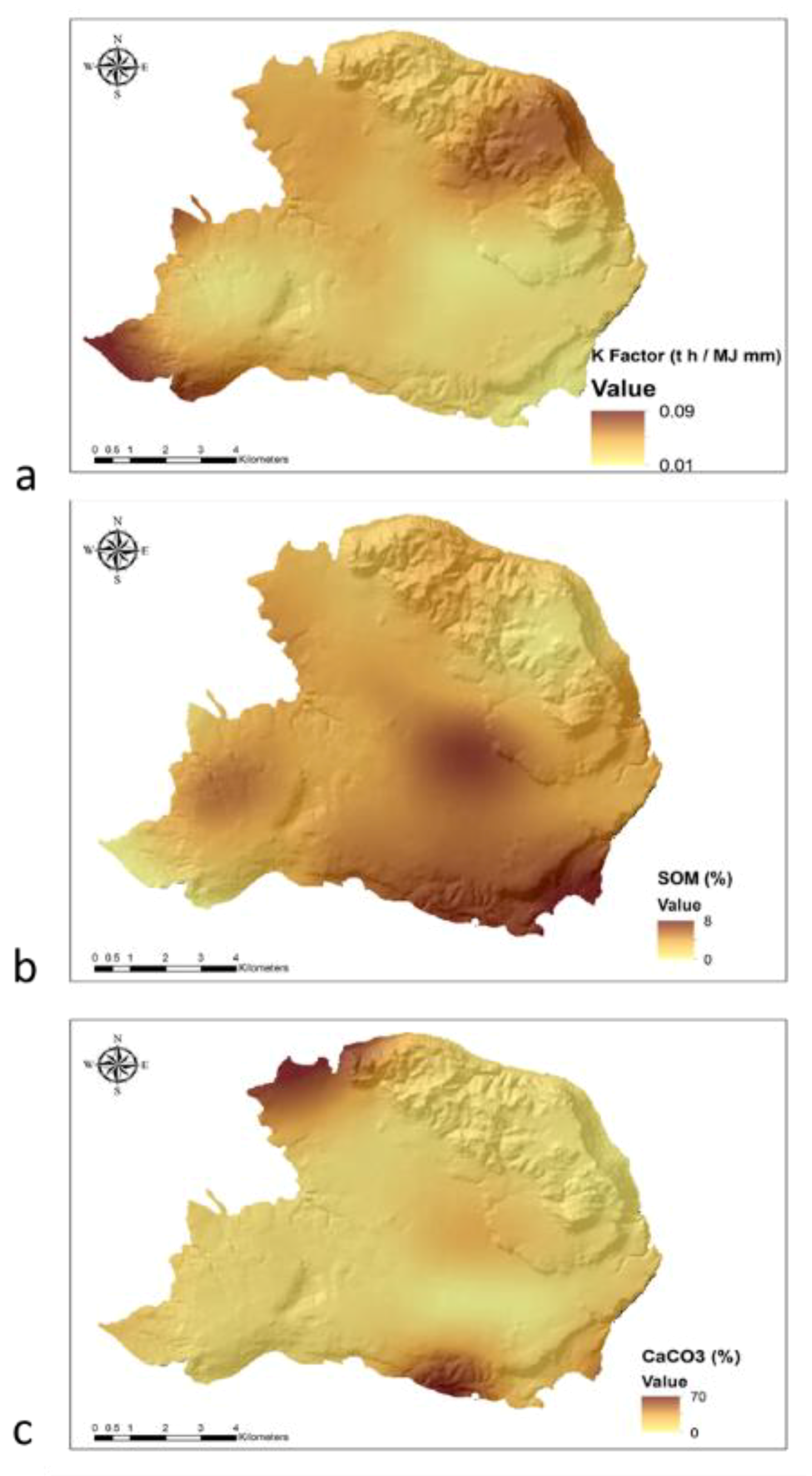
Initially, after the estimation of SOM and CaCO₃ parameters, through laboratory soil samples analysis, K-factor was calculated using Equation (1) in the GIS environment. The maps denote a conceptual uncertainty in the values distribution of all three parameters (Figure 6a–c). This uncertainty was also depicted in the statistical results in terms of spline methodology accuracy. Specifically, 20 random point measurements were selected for applying the interpolation method and 10 points for validating the results. The extremely low R² values, as estimated for correlating training and validating measurements and concerning all the estimated parameters (SOM, CaCO₃, and K-factor), highlighted the need for developing a new coherent methodology for explicitly mapping soil parameters with the use of EO data. These results are merely in accordance with similar studies [49] that applied the Ordinary kriging method to estimate SOM.

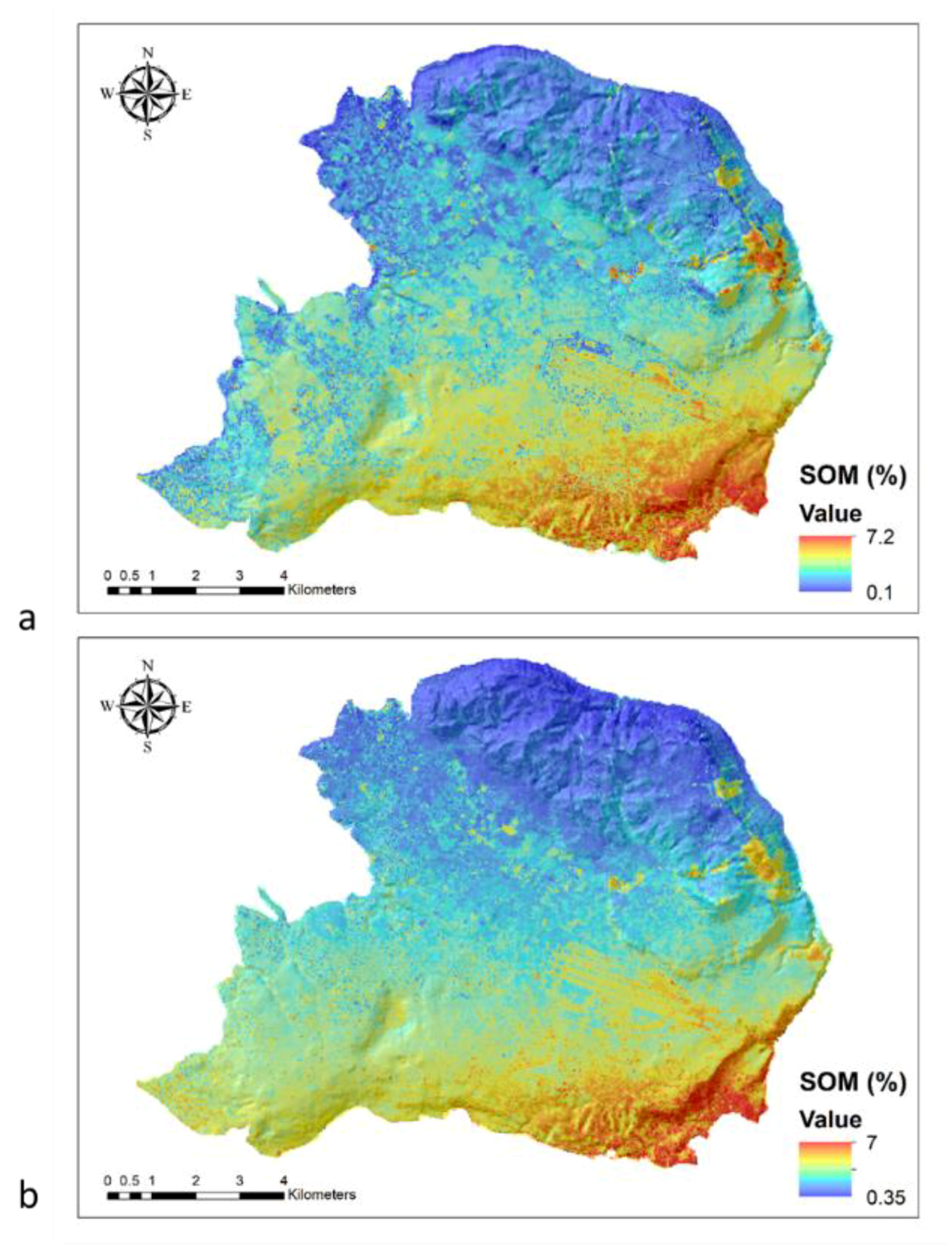
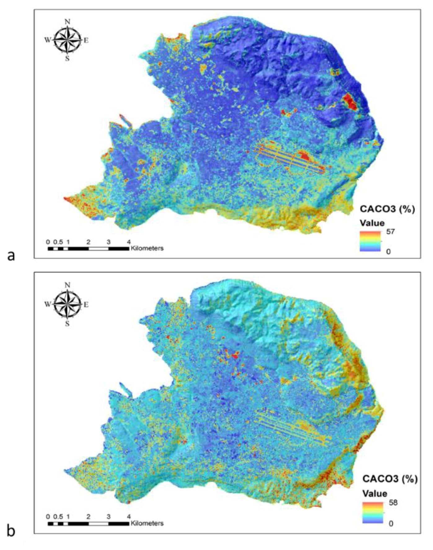
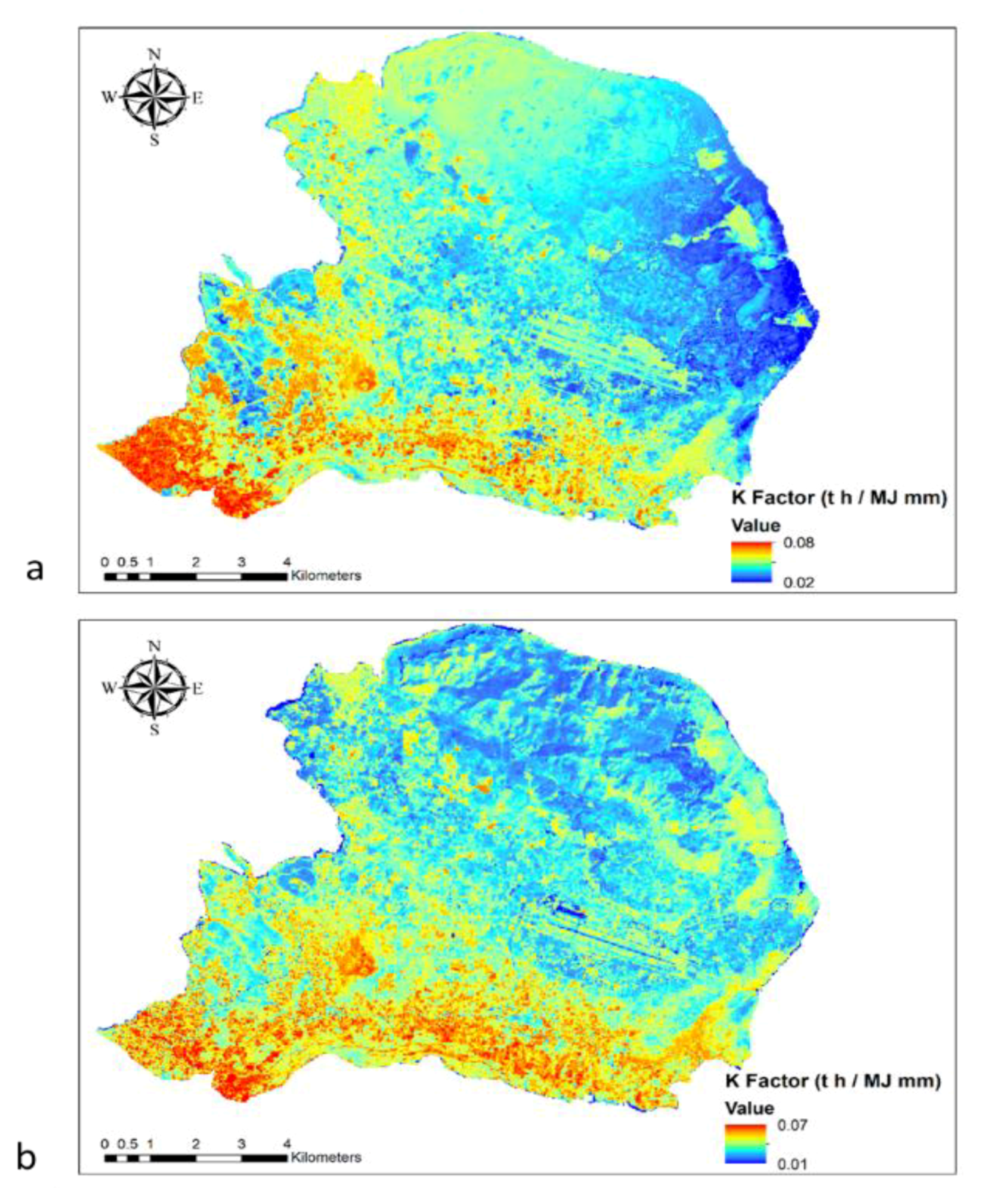
Following this, three individual maps were constructed from the synergistic use of ANN, satellite data, and laboratory analysis, modeling the SOM, the CaCO₃, and the K-factor, respectively. Specifically, the integration of the different approaches contributed to the development of six different maps concerning both satellite sensors, Sentinel-2 and Landsat 8 (Figure 7a,b, Figure 8a,b, and Figure 9a,b). Furthermore, the ANN MLP simulation results produced good agreement with those measured in the field data in terms of R² and root-mean-square error (RMSE) (

Table 3. Statistics of R² and root-mean-square error (RMSE) concerning the performance of the MLP artificial neural network (ANN) algorithm in the Landsat 8 data.

Landsat 8
	Mean RMSE				Mean R2
	Training	Testing	Validation	Overall	Training	Testing	Validation	Overall
SOM	0.55	1.1	0.67	0.58	0.88	0.52	0.83	0.87
CaCO3	6.5	9.2	7.3	8.08	0.84	0.5	0.6	0.79
K-factor	0.0087	0.016	0.01	0.0095	0.7	0.42	0.52	0.6

and

Table 4. Statistics of R² and RMSE concerning the performance of the MPL ANN algorithm in the Sentinel-2 data.

Sentinel-2
	Mean RMSE				Mean R2
	Training	Testing	Validation	Overall	Training	Testing	Validation	Overall
SOM	0.43	1.1	0.94	0.58	0.93	0.41	0.67	0.87
CaCO3	6.3	10.1	8.4	7.1	0.85	0.56	0.74	0.82
K-factor	0.002	0.0164	0.0114	0.0093	0.68	0.39	0.42	0.59

) for both Landsat 8 and Sentinel-2 satellite imageries.

In most cases, the results were within an acceptable range considering the complexity of the case study and the limited data availability. For both datasets, the SOM parameter was better simulated by the ANNs, which was expected since the dataset used was more diverse and its statistical characteristics were well distributed. In addition, these results in terms of R² were in accordance with the results of [50], who estimated SOM with the use of ANN and remote sensing data. For the calculation of the K-factor, both SOM and CaCO₃ data were used (see Equation (1)), thus the uncertainty derived by both datasets was accumulated to the K-factor dataset, resulting in the worst simulation results amongst the three parameters simulated. However, because the study system was quite complex, the simulation was considered successful.

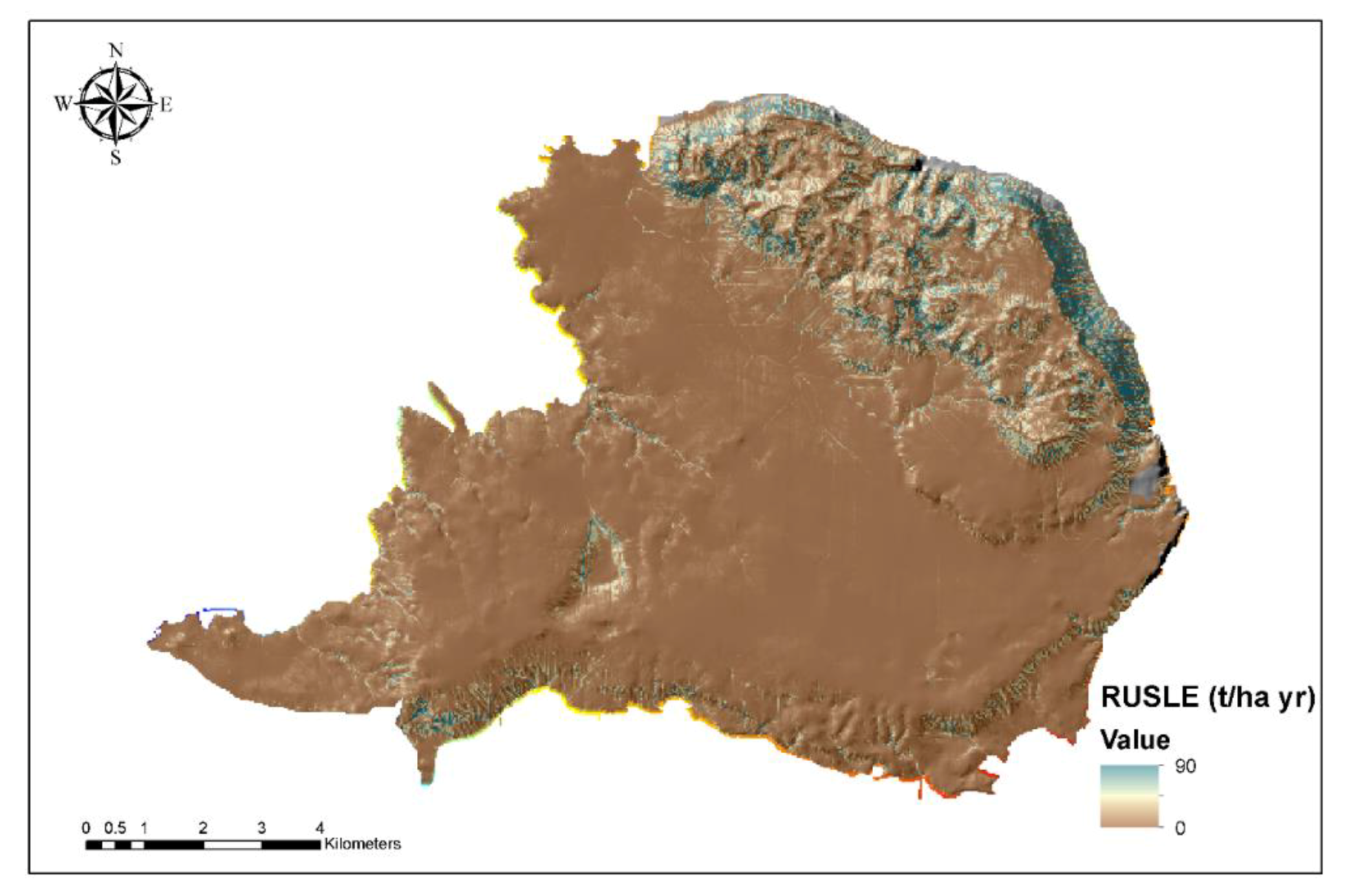
Using the RUSLE model, the final soil erosion map of the Akrotiri cape was developed (Figure 10). The results denote high soil erosion risk in the northeastern part of the cape, where steep slopes occur. Specifically, an average soil loss rate of more than 80 $t h{a}^{-1}yea{r}^{-1}$ was recorded for 2018 in the specific area.

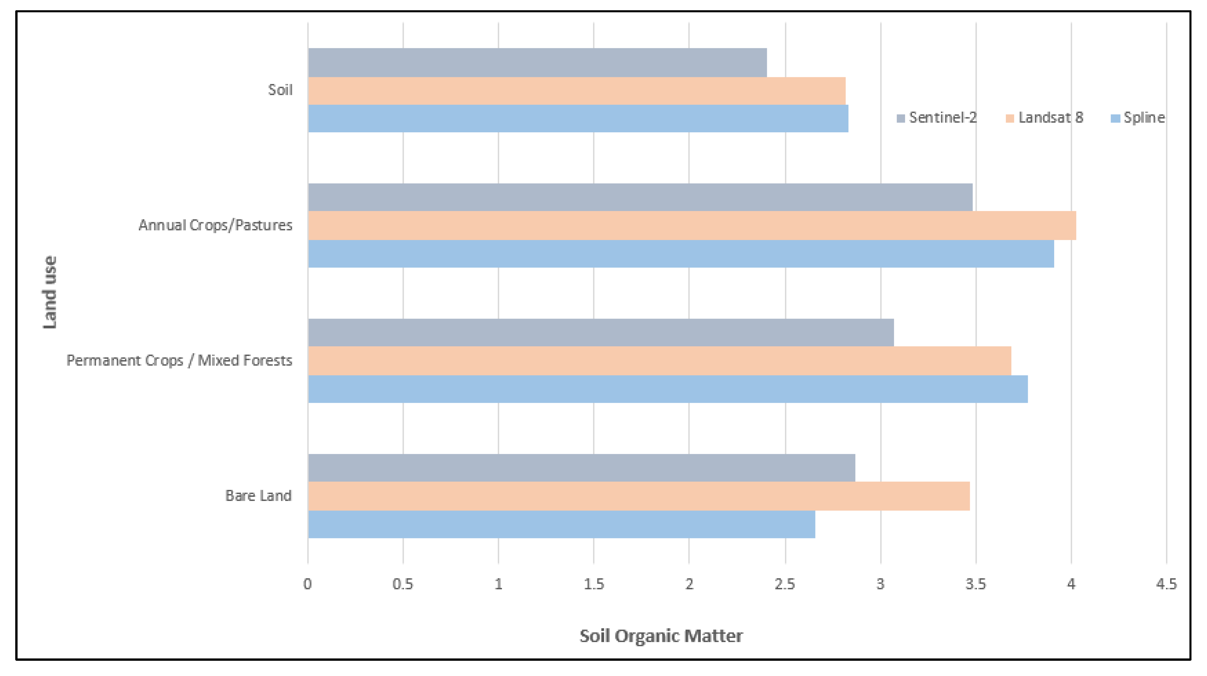
The study area was divided to four different land use classes according to CORINE 2006 land cover data, and zonal statistics were calculated in terms of SOM content using different methodological approaches (Spline interpolation, Sentinel-2, and Landsat-8). The results denote the trend of the Sentinel-2 methodology to underestimate SOM values compared to the Spline and the Landsat 8 approaches (Figure 11).

The study area was divided according to topography and the RUSLE results into affected (>50 m height) and no erosion-affected areas (<50 m height). The affected areas were delineated in the northeastern part of the cape where high slope inclinations occur, and corresponding high soil loss rates were recorded (approximately 80 $t h{a}^{-1}yea{r}^{-1}$). The less erosion prone areas were delineated in the almost flat areas in the central part of the cape, where minimum soil loss rates (~6 $t h{a}^{-1}yea{r}^{-1}$) were recorded.

Table 5. Statistical results of SOM and the RUSLE correlation

	Erosion Affected Areas		No Erosion Affected Areas
	Mean SOM (%)	St. Deviation	Mean SOM (%)	St. Deviation
Spline	1.84	0.3	4.4	0.78
Landsat 8	1.76	0.92	3.4	0.98
Sentinel-2	2.15	0.3	3.69	0.78

indicates the statistical correlation between soil loss rates and SOM measurements in the above-mentioned areas. The results highlight the fact that the average SOM deposits decrease in areas that suffer from water soil erosion due to the phenomenon of topsoil removal.

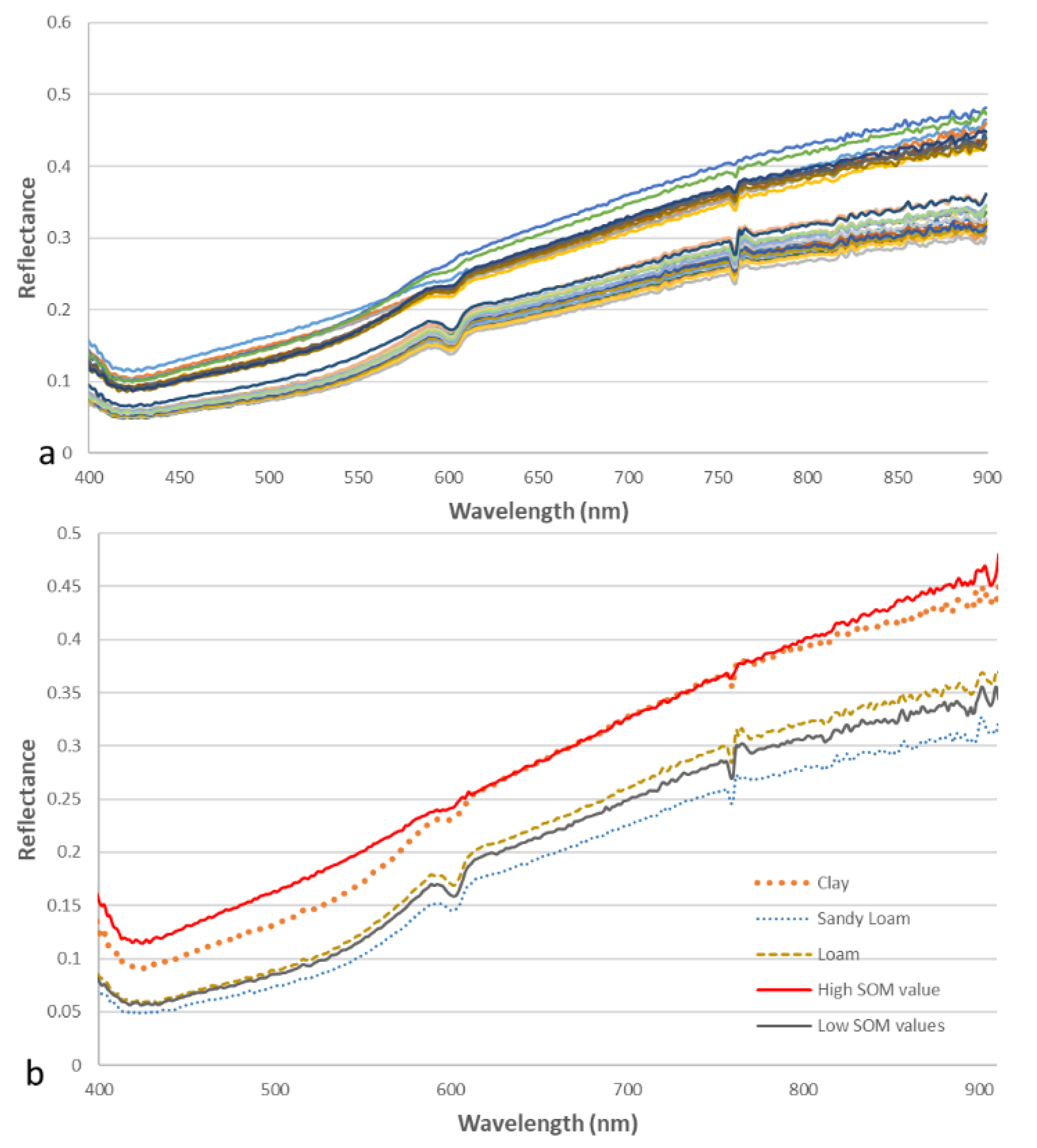
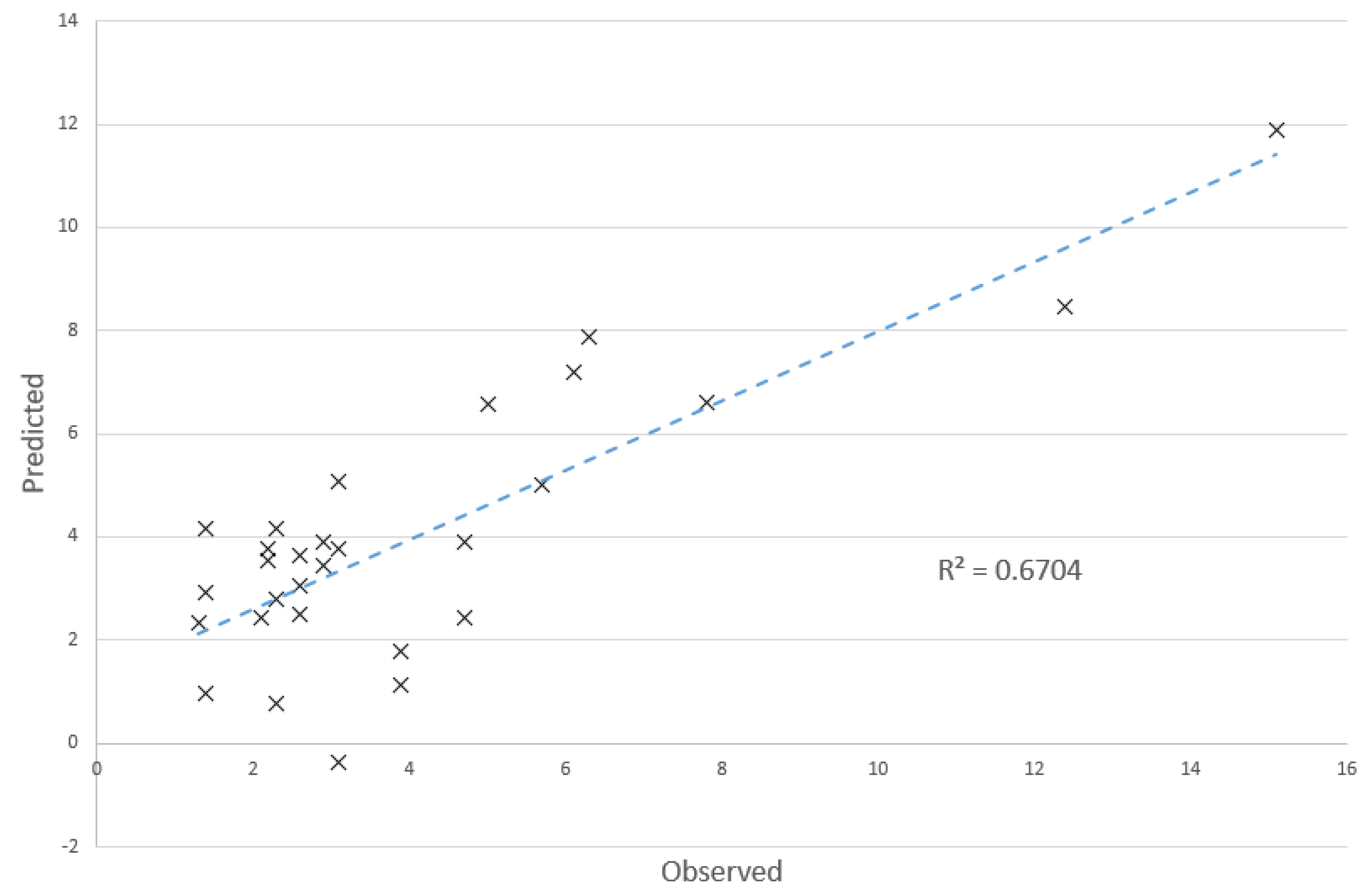
Following this, the OLSR methodology was applied to correlate the SOM parameter with the soil samples’ corresponding spectral signatures, as derived from field spectroscopy campaigns. As it was previously stated, in case there is an initial filtering of the vast number of the available spectral bands, the field spectroscopy can be a valuable tool in modeling and predicting soil parameters with means of spectral analysis. The value of R² = 0.67, as indicated in Figure 12, is promising for actively incorporating field spectroscopy in soil studies.

The results concerning the application of the GWR methodology for comparing the RUSLE, the slope inclination (degrees), and the SOM datasets in terms of R² are presented in

Table 6. R² statistics and slope inclination results concerning cross comparison between real data and the RUSLE results with various SOM estimation approaches.

SOM	R Square
	RUSLE (Soil Loss)	Inclination (Degrees)
Spline	0.08	0.99
Landsat 8	0.41	0.80
Sentinel-2	0.29	0.88

.

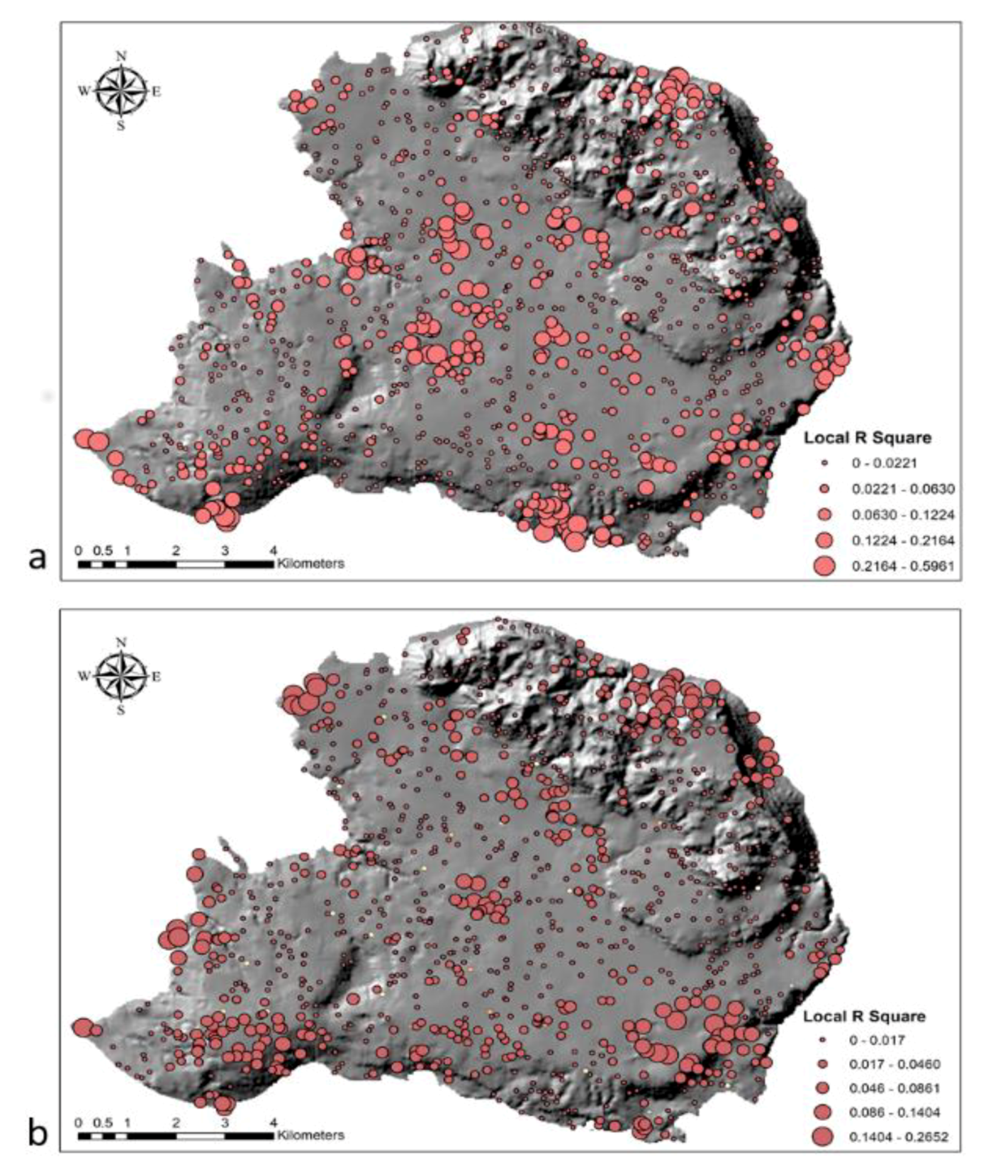
The R² values describe the overall fit of the developed models. The results denote the ultimate correlation of SOM with the terrain morphology in terms of slope inclination. On the other hand, the low R² values concerning comparison of the soil loss model with the SOM parameter highlight the multi-parametric nature of the soil erosion phenomenon, which cannot be actually described with the employment of a unique variable such as SOM. In Figure 13, the overall spatial allocation of local R² values concerning the correlation between the RUSLE and the ANN satellite derived SOM products is presented. It seems that Landsat 8 had greater spatial allocation of high R² values across the study area (Figure 13a).

5. Conclusions

Greece is a Mediterranean Europe hotspot extremely prone to soil erosion. Both Mediterranean land managers and stakeholders need sound, evidence-based information about land degradation patterns and the effectiveness of their management responses [8]. Obtaining such information, however, is particularly difficult in Mediterranean grazing lands, where a long history of anthropogenic pressure, high topographical and climatic variability, and frequent disturbances combine to create a highly diverse and unstable environment.

This paper highlights the significance of determining the soil erosion threat using both EO and field spectral VIS-NIR data in order to monitor soil regime and adopt the appropriate measures and practices for soil conservation and sustainable land use. Furthermore, the manuscript highlights the potential of the ANN inversion model for the estimation of the soil erosion phenomenon with the use of EO data. The collection of crucial in situ soil parameters data such as SOM and CaCO₃ in remote areas is often an impractical, expensive, and time-consuming process; therefore, the development of alternative data collection methodologies is indispensable. In this context, efficient spatial simulations of the crucial soil parameters, SOM and CaCO₃, were carried out using field spectral VIS-NIR measurements and satellite remote sensing observations (Sentinel-2 and Landsat 8) combined with non-linear (ANNs) approaches. The derived maps successfully captured the SOM and the CaCO₃ spatial distribution in the GIS environment (approximately 80% R² for images from both sensors). It is important to state that the results are optimum for SOM compared to CaCO₃. Accordingly, the aforementioned maps were used for the spatial estimation of K-factor, which formed the main data input in the RUSLE model to estimate the soil erosion risk in the study area. The results depicted increased soil erosion risk in the northeastern part of the Akrotiri cape, where steep slopes occur. In addition, field spectroscopy data were collected for various soil samples, and statistical analysis (OLSR and GWR) was carried out to compare them to relevant soil parameters (SOM and CaCO₃) values. The high corresponding R² values (67%) for OLSR denoted the potential of field spectroscopy to describe soil health effectively. Finally, the results highlighted the fact that the terrain morphology is absolutely related to soil erosion rates rather than SOM values that cannot successfully describe the soil erosion regime.

The presented approach forms a sufficient methodology for incorporating EO data in monitoring soil parameters and consequently estimating soil erosion. Results demonstrate that the retrieval of soil parameters is possible by using satellite data, either Sentinel-2 or Landsat 8, and an inversion algorithm, making the whole process both time and cost efficient. This overall approach will contribute to the design of good soil erosion management practices and wise land use planning in the study region or wherever it is needed. In addition, this work can provide significant guidelines for defining and monitoring additional areas susceptible to soil erosion. Future research will focus on further data collection in broader areas for a more accurate validation of the results.

References

1. Lal, R. Soil erosion and the global carbon budget. Environ. Int. 2003, 29, 437–450. [Google Scholar] [CrossRef] [Green Version]
2. Chiemelu, N.; Okeke, F.; Nwosu, K.; Ibe, C.; Ndukwu, R.; Ugwuoti, A. The Role of Surveying and Mapping in Erosion Management and Control: Case of Omagba Erosion Site, Onitsha Anambra State, Nigeria. J. Environ. Earth Sci. 2013, 3, 129–137. [Google Scholar]
3. Module 4: Soils and their management for Climate-smart Agriculture. Available online: http://www.fao.org/3/i3325e/i3325e00.htm (accessed on 7 May 2019).
4. Panagos, P.; Standardi, G.; Borrelli, P.; Lugato, E.; Montanarella, L.; Bosello, F. Cost of agricultural productivity loss due to soil erosion in the European Union: From direct cost evaluation approaches to the use of macroeconomic models. Land Degrad. Dev. 2018, 29, 471–484. [Google Scholar] [CrossRef] [Green Version]
5. Montanarella, L. Trends in Land Degradation in Europe. In Climate and Land Degradation; Springer: Berlin/Heidelberg, Germany, 2007; pp. 83–104. [Google Scholar]
6. Kouli, M.; Soupios, P.; Vallianatos, F. Soil erosion prediction using the Revised Universal Soil Loss Equation (RUSLE) in a GIS framework, Chania, Northwestern Crete, Greece. Environ. Geol. 2009, 57, 483–497. [Google Scholar] [CrossRef]
7. Kourgialas, N.N.; Koubouris, G.C. Assessing water erosion in Mediterranean tree crops using GIS techniques and field measurements: The effect of climate change. Nat. Hazards 2016, 83, 65–81. [Google Scholar] [CrossRef]
8. Jucker Riva, M.; Daliakopoulos, I.N.; Eckert, S.; Hodel, E.; Liniger, H. Assessment of land degradation in Mediterranean forests and grazing lands using a landscape unit approach and the normalized difference vegetation index. Appl. Geogr. 2017, 86, 8–21. [Google Scholar] [CrossRef]
9. Kosmas, C.; Detsis, V.; Karamesouti, M.; Kounalaki, K.; Vassiliou, P.; Salvati, L.; Kosmas, C.; Detsis, V.; Karamesouti, M.; Kounalaki, K.; et al. Exploring Long-Term Impact of Grazing Management on Land Degradation in the Socio-Ecological System of Asteroussia Mountains, Greece. Land 2015, 4, 541–559. [Google Scholar] [CrossRef] [Green Version]
10. Conforti, M.; Buttafuoco, G.; Leone, A.P.; Aucelli, P.P.C.; Robustelli, G.; Scarciglia, F. Studying the relationship between water-induced soil erosion and soil organic matter using Vis-NIR spectroscopy and geomorphological analysis: A case study in southern Italy. Catena 2013, 110, 44–58. [Google Scholar] [CrossRef]
11. Vasques, G.M.; Grunwald, S.; Comerford, N.B.; Sickman, J.O. Regional modelling of soil carbon at multiple depths within a subtropical watershed. Geoderma 2010, 156, 326–336. [Google Scholar] [CrossRef]
12. Walker, E.; Monestiez, P.; Gomez, C.; Lagacherie, P. Combining measured sites, soilscapes map and soil sensing for mapping soil properties of a region. Geoderma 2017, 300, 64–73. [Google Scholar] [CrossRef] [Green Version]
13. Ostovari, Y.; Ghorbani-Dashtaki, S.; Bahrami, H.A.; Abbasi, M.; Dematte, A.M.; Arthur, E.; Panagos, P. Towards prediction of soil erodibility, SOM and CaCO3using laboratory Vis-NIR spectra: A case study in a semi-arid region of Iran. Geoderma 2018, 314, 102–112. [Google Scholar] [CrossRef]
14. Hill, J.; Hostert, P.; Tsiourlis, G.; Kasapidis, P.; Udelhoven, T.; Diemer, C. Monitoring 20 years of increased grazing impact on the Greek island of Crete with earth observation satellites. J. Arid Environ. 1998, 39, 165–178. [Google Scholar] [CrossRef]
15. Ganasri, B.P.; Ramesh, H. Assessment of soil erosion by RUSLE model using remote sensing and GIS—A case study of Nethravathi Basin. Geosci. Front. 2016, 7, 953–961. [Google Scholar] [CrossRef]
16. Cheng, Z.; Lu, D.; Li, G.; Huang, J.; Sinha, N.; Zhi, J.; Li, S.; Cheng, Z.; Lu, D.; Li, G.; et al. A Random Forest-Based Approach to Map Soil Erosion Risk Distribution in Hickory Plantations in Western Zhejiang Province, China. Remote Sens. 2018, 10, 1899. [Google Scholar] [CrossRef]
17. Puente, C.; Olague, G.; Trabucchi, M.; Arjona-Villicaña, P.; Soubervielle-Montalvo, C.; Puente, C.; Olague, G.; Trabucchi, M.; Arjona-Villicaña, P.D.; Soubervielle-Montalvo, C. Synthesis of Vegetation Indices Using Genetic Programming for Soil Erosion Estimation. Remote Sens. 2019, 11, 156. [Google Scholar] [CrossRef]
18. Conforti, M.; National, I.; Buttafuoco, G.; National, I.; Leone, A.P.; National, I.; Aucelli, P. Soil erosion assessment using proximal spectral reflectance in VIS-NIR-SWIR region in sample area of Calabria region (southern Italy). Rendiconti Online della Società Geologica Italiana 2012, 21, 1202–1204. [Google Scholar]
19. Wischmeier, W.H.; Smith, D.D. 1905- Predicting rainfall-erosion losses from cropland east of the Rocky Mountains. USDA Agric. Res. Serv. Handb. 1965, 2, 82. [Google Scholar]
20. Renard, K.G.; Agricultural Research Service; Foster, G.R.; Weesies, G.A.; McCool, D.K.; Yoder, D.C. Predicting Soil Erosion by Water: A Guide to Conservation Planning with the Revised Universal Soil Loss Equation (RUSLE); United States Department of Agriculture: Washington, DC, USA, 1997.
21. Renard, K.G.; Freimund, J.R. Using monthly precipitation data to estimate the R-factor in the revised USLE. J. Hydrol. 1994, 157, 287–306. [Google Scholar] [CrossRef]
22. Gaubi, I.; Chaabani, A.; Ben Mammou, A.; Hamza, M.H. A GIS-based soil erosion prediction using the Revised Universal Soil Loss Equation (RUSLE) (Lebna watershed, Cap Bon, Tunisia). Nat. Hazards 2017, 86, 219–239. [Google Scholar] [CrossRef]
23. Alexakis, D.D.; Hadjimitsis, D.G.; Agapiou, A. Integrated use of remote sensing, GIS and precipitation data for the assessment of soil erosion rate in the catchment area of “Yialias” in Cyprus. Atmos. Res. 2013, 131, 108–124. [Google Scholar] [CrossRef]
24. Borrelli, P.; Märker, M.; Panagos, P.; Schütt, B. Modeling soil erosion and river sediment yield for an intermountain drainage basin of the Central Apennines, Italy. CATENA 2014, 114, 45–58. [Google Scholar] [CrossRef]
25. Thomas, J.; Joseph, S.; Thrivikramji, K.P. Assessment of soil erosion in a monsoon-dominated mountain river basin in India using RUSLE-SDR and AHP. Hydrol. Sci. J. 2018, 63, 542–560. [Google Scholar] [CrossRef]
26. Phinzi, K.; Ngetar, N.S. The assessment of water-borne erosion at catchment level using GIS-based RUSLE and remote sensing: A review. Int. Soil Water Conserv. Res. 2018, 7, 27–46. [Google Scholar] [CrossRef]
27. Kim, M.; Gilley, J.E. Artificial Neural Network estimation of soil erosion and nutrient concentrations in runoff from land application areas. Comput. Electron. Agric. 2008, 64, 268–275. [Google Scholar] [CrossRef] [Green Version]
28. Gholami, V.; Booij, M.J.; Nikzad Tehrani, E.; Hadian, M.A. Spatial soil erosion estimation using an artificial neural network (ANN) and field plot data. Catena 2018, 163, 210–218. [Google Scholar] [CrossRef]
29. Rahmati, O.; Tahmasebipour, N.; Haghizadeh, A.; Pourghasemi, H.R.; Feizizadeh, B. Evaluation of different machine learning models for predicting and mapping the susceptibility of gully erosion. Geomorphology 2017, 298, 118–137. [Google Scholar] [CrossRef]
30. Panagos, P.; Meusburger, K.; Ballabio, C.; Borrelli, P.; Alewell, C. Soil erodibility in Europe: A high-resolution dataset based on LUCAS. Sci. Total Environ. 2014, 479–480, 189–200. [Google Scholar] [CrossRef]
31. Alexakis, D.D.; Sarris, A. Integrated GIS and remote sensing analysis for landfill sitting in Western Crete, Greece. Environ. Earth Sci. 2014, 72, 467–482. [Google Scholar] [CrossRef]
32. Agapiou, A.; Alexakis, D.D.; Sarris, A.; Hadjimitsis, D.G. Linear 3-D transformations of Landsat 5 TM satellite images for the enhancement of archaeological signatures during the phenological cycle of crops. Int. J. Remote Sens. 2015, 36, 20–35. [Google Scholar] [CrossRef]
33. Bouyoucos, G.J. Hydrometer Method Improved for Making Particle Size Analyses of Soils1. Agron. J. 1962, 54, 464. [Google Scholar] [CrossRef]
34. Doubková, M.; Van Dijk, A.I.J.M.; Sabel, D.; Wagner, W.; Blöschl, G. Evaluation of the predicted error of the soil moisture retrieval from C-band SAR by comparison against modelled soil moisture estimates over Australia. Remote Sens. Environ. 2012, 120, 188–196. [Google Scholar] [CrossRef] [Green Version]
35. Walkley, A.; Black, I.A. An examination of the Degtjareff method for determining soil organic matter, and a proposed modification of the chromic acid titration method. Soil Sci. 1934, 37, 29–37. [Google Scholar] [CrossRef]
36. Bannari, A.; El-Battay, A.; Bannari, R.; Rhinane, H. Sentinel-MSI VNIR and SWIR Bands Sensitivity Analysis for Soil Salinity Discrimination in an Arid Landscape. Remote Sens. 2018, 10, 855. [Google Scholar] [CrossRef]
37. Yue, Y.; Sun, J.; Liu, X.; Ren, D.; Liu, Q.; Xiao, X.; Lu, L. Spatial analysis of dengue fever and exploration of its environmental and socio-economic risk factors using ordinary least squares: A case study in five districts of Guangzhou City, China, 2014. Int. J. Infect. Dis. 2018, 75, 39–48. [Google Scholar] [CrossRef]
38. Haykin, S.S.; Simon, S. Neural Networks: A Comprehensive Foundation; Prentice Hall: Upper Saddle River, NJ, USA, 1999. [Google Scholar]
39. Tapoglou, E.; Karatzas, G.P.; Trichakis, I.C.; Varouchakis, E.A. A spatio-temporal hybrid neural network-Kriging model for groundwater level simulation. J. Hydrol. 2014, 519, 3193–3203. [Google Scholar] [CrossRef]
40. Kia, M.B.; Pirasteh, S.; Pradhan, B.; Mahmud, A.R.; Sulaiman, W.N.A.; Moradi, A. An artificial neural network model for flood simulation using GIS: Johor River Basin, Malaysia. Environ. Earth Sci. 2012, 67, 251–264. [Google Scholar] [CrossRef]
41. Santi, E.; Paloscia, S.; Pettinato, S.; Fontanelli, G. Application of artificial neural networks for the soil moisture retrieval from active and passive microwave spaceborne sensors. Int. J. Appl. Earth Obs. Geoinf. 2015, 48, 61–73. [Google Scholar] [CrossRef]
42. Daliakopoulos, I.N.; Coulibaly, P.; Tsanis, I.K. Groundwater level forecasting using artificial neural networks. J. Hydrol. 2005, 309, 229–240. [Google Scholar] [CrossRef]
43. Angima, S.; Stott, D.; O’Neill, M.; Ong, C.; Weesies, G. Soil erosion prediction using RUSLE for central Kenyan highland conditions. Agric. Ecosyst. Environ. 2003, 97, 295–308. [Google Scholar] [CrossRef]
44. Panagos, P.; Borrelli, P.; Meusburger, K.; Alewell, C.; Lugato, E.; Montanarella, L. Estimating the soil erosion cover-management factor at the European scale. Land Use Policy 2015, 48, 38–50. [Google Scholar] [CrossRef] [Green Version]
45. Moore, I.D.; Burch, G.J. Physical Basis of the Length-slope Factor in the Universal Soil Loss Equation1. Soil Sci. Soc. Am. J. 1986, 50, 1294. [Google Scholar] [CrossRef]
46. See, L.; Schepaschenko, D.; Lesiv, M.; McCallum, I.; Fritz, S.; Comber, A.; Perger, C.; Schill, C.; Zhao, Y.; Maus, V.; et al. Building a hybrid land cover map with crowdsourcing and geographically weighted regression. ISPRS J. Photogramm. Remote Sens. 2015, 103, 48–56. [Google Scholar] [CrossRef] [Green Version]
47. Zhou, Q.; Wang, C.; Fang, S. Application of geographically weighted regression (GWR) in the analysis of the cause of haze pollution in China. Atmos. Pollut. Res. 2018, 10, 835–846. [Google Scholar] [CrossRef]
48. Johnson, B.A.; Scheyvens, H.; Baqui Khalily, M.A.; Onishi, A. Investigating the relationships between climate hazards and spatial accessibility to microfinance using geographically-weighted regression. Int. J. Disaster Risk Reduct. 2018, 33, 122–130. [Google Scholar] [CrossRef]
49. Chabala, L.M.; Mulowa, A.; Lungu, O. Application of Ordinary Kriging in Mapping Soil Organic Carbon in Zambia. Pedosphere 2017, 27, 338–343. [Google Scholar] [CrossRef]
50. Ayoubi, S.; Pilehvar, A.; Mokhtari, P.; Sahrawat, K. Application of Artificial Neural Network (ANN) to Predict Soil Organic Matter Using Remote Sensing Data in Two Ecosystems. In Biomass and Remote Sensing of Biomass; InTech: Rijeka, Croatia, 2011. [Google Scholar] [Green Version]
Figure 1. Study area.
Remotesensing 11 01106 g001
Figure 2. Landsat 8 (up) and Sentinel-2 (down) natural color composites [(Landsat 8 RGB: 432, 30 m spatial resolution), (Sentinel-2 RGB: 432, 10 m spatial resolution)] and corresponding sampling points allocation. RGB= red, green, blue.
Remotesensing 11 01106 g002
Figure 3. The United States Department of Agriculture (USDA) textural distribution of the soils at the study site.
Remotesensing 11 01106 g003
Figure 4. Flowchart of the overall methodology.
Remotesensing 11 01106 g004
Figure 5. (a) Spectral reflectance response of soil samples as derived from spectroradiometer. (b) Soil sample soil organic matter (SOM) values and texture analysis in terms of spectral reflectance (mean values).
Remotesensing 11 01106 g005
Figure 6. (a) Soil erodibility (K-factor), (b) SOM, and (c) CaCO3 spatial distribution in the study area.
Remotesensing 11 01106 g006
Figure 7. Spatial distribution of SOM as estimated from the integrated use of ANN and Landsat 8 (a) and Sentinel-2 (b) imageries.
Remotesensing 11 01106 g007
Figure 8. Spatial distribution of CaCO3 as estimated from the integrated use of ANN and Landsat 8 (a), and Sentinel-2 (b) imageries.
Remotesensing 11 01106 g008
Figure 9. Spatial distribution of K-factor as estimated from the integrated use of ANN and (a) Landsat 8, and (b) Sentinel-2 imageries.
Remotesensing 11 01106 g009
Figure 10. Soil erosion [Revised Universal Soil Loss Equation (RUSLE)] map of the study area.
Remotesensing 11 01106 g010
Figure 11. SOM spatial distribution according to Land Use/Land Classes.
Remotesensing 11 01106 g011
Figure 12. Scatterplot of predicted versus measured values for the SOM parameter.
Remotesensing 11 01106 g012
Figure 13. Spatial allocation of local R2 values concerning the correlation between the RUSLE and the ANN satellite derived SOM for (a) Landsat 8, and (b) Sentinel-2 imageries.
Remotesensing 11 01106 g013