Tree Height Estimation of Forest Plantation in Mountainous Terrain from Bare-Earth Points Using a DoG-Coupled Radial Basis Function Neural Network

Abstract

Tree heights are the principal variables for forest plantation inventory. The increasing availability of high-resolution three-dimensional (3D) point clouds derived from low-cost Unmanned Aerial Vehicle (UAV) and modern photogrammetry offers an opportunity to generate a Canopy Height Model (CHM) in the mountainous areas. In this paper, we assessed the capabilities of tree height estimation using UAV-based Structure-from-Motion (SfM) photogrammetry and Semi-Global Matching (SGM). The former is utilized to generate 3D geometry, while the latter is used to generate dense point clouds from UAV imagery. The two algorithms were coupled with a Radial Basis Function (RBF) neural network to acquire CHMs in mountainous areas. This study focused on the performance of Digital Terrain Model (DTM) interpolation over complex terrains. With the UAV-based image acquisition and image-derived point clouds, we constructed a 5 cm-resolution Digital Surface Model (DSM), which was assessed against 14 independent checkpoints measured by a Real-Time Kinematic Global Positioning System RTK GPS. Results showed that the Root Mean Square Errors (RMSEs) of horizontal and vertical accuracies are approximately 5 cm and 10 cm, respectively. Bare-earth Index (BEI) and Shadow Index (SI) were used to separate ground points from the image-derived point clouds. The RBF neural network coupled with the Difference of Gaussian (DoG) was exploited to provide a favorable generalization for the DTM from 3D ground points with noisy data. CHMs were generated using the height value in each pixel of the DSM and by subtracting the corresponding DTM value. Individual tree heights were estimated using local maxima algorithm under a contour-surround constraint. Two forest plantations in mountainous areas were selected to evaluate the accuracy of estimating tree heights, rather than field measurements. Results indicated that the proposed method can construct a highly accurate DTM and effectively remove nontreetop maxima. Furthermore, the proposed method has been confirmed to be acceptable for tree height estimation in mountainous areas given the strong linear correlation of the measured and estimated tree heights and the acceptable t-test values. Overall, the low-cost UAV-based photogrammetry and RBF neural network can yield a highly accurate DTM over mountainous terrain, thereby making them particularly suitable for rapid and cost-effective estimation of tree heights of forest plantation in mountainous areas.

1. Introduction

In remote mountainous areas of China with complex terrain, the maturity of trees varies due to differences in climate or fertility. Many forest plantations are difficult to be uniformly planted or felled. The felling of trees is typically determined by variables, such as the height and Diameter at Breast Height (DBH). Deforested areas are frequently unevenly distributed and replanted on the basis of the growing environment of the forest plantations. Therefore, the rapid and low-cost acquisition of tree heights and other variables is crucial. Individual tree height is an important variable in forest inventory and useful for silvicultural treatments and management of timber production. This variable can provide a decision-making reference for deforestation and planting trees, including deciding on the locations for clear-felling and tree planting depending on the site inventory and distribution of trees, correspondingly.

Remote sensing technology is broadly used in various applications for forest investigation; these applications include forest growth, forest quality prediction, and refined management of forests [1,2]. Satellite remote sensing images, including multiband spectral information, can be used to establish high-precision forest parameter inversion regression models that are useful for large areas but unsuitable for extracting refined individual trees because multispectral or hyperspectral remote sensing images only have a meter or submeter resolution. Satellite remote sensing also suffers from the limitations of acquisition time and weather conditions, and remote sensing-based approaches are inconsiderably effective to accurately estimate the height and canopy of individual trees [3,4].

In comparison with satellite remote sensing, Unmanned Aerial Vehicle (UAV)-based photogrammetry, with the advantage of low-cost and flexible operation, can concurrently acquire high-resolution remotely sensed images and derive high-accuracy dense point clouds; thus, it is especially suitable for the rapid periodic inventory of forest plantations by estimating tree heights and crowns. Furthermore, UAV-based photogrammetry is suited for data acquisition of forest and small classes; this method not only focuses on individual trees or sample plots but also is feasible for monitoring forest stands that make UAV technology a significant advantage in forest resource survey and dynamic monitoring. In contrast to traditional field measurements, UAV-based forest inventory can be separated from the traditional site survey conducted using sample plots. On the basis of the UAV-based photogrammetric mapping, any area within the scope of forest plantation that must be monitored can be surveyed from the photogrammetric results, rather than field measurement. Thus, the efficiency is much better in forest investigation than in traditional forest survey methods. The development of UAV and related technologies has promoted the application in forest inventory, and the demand for modern forestry survey has increased the research on drones in forestry. UAV-equipped camera and laser sensors have also been exploited for tree height estimation.

UAV-based approaches for tree heights estimation can be classified into the following categories based on equipped sensors, namely, (1) image-based approaches, (2) LiDAR point cloud-based approaches, and (3) image and LiDAR point cloud-integrated approaches. Puliti et al. [5] used Agisoft software (version, Manufacturer, City, US State abbrev. if applicable, Country) to obtain dense point clouds of the study area from UAV images and established a linear regression model based on ground data to estimate the number of trees, average tree height, dominant tree species height, and cross-sectional area at breast height in Southeastern Norway. Zarco-Tejada et al. [6] used UAV to generate a 3D Digital Surface Model (DSM) to estimate tree height; in addition, the correlation coefficient with the field-measured tree height exceeded 0.8. Jing et al. [7] improved a multiscale image segmentation algorithm to obtain a high-quality canopy map through Gaussian filtering and a watershed algorithm. Chianucci et al. [8] used UAV images obtained by a consumer-grade camera to perform a large-scale estimation of forest canopy attributes, objectively evaluated the forest canopy coverage, and computed the leaf area index [9]. Panagiotidis et al. [10] reconstructed 3D ground structures from UAV image sequences for two study areas and extracted the heights and canopy diameters of dominant trees. In addition, a UAV laser scanner can capture LiDAR point cloud for accurate access to forest structure parameters. Studies have shown that UAV-based photogrammetry lacks the ability to penetrate dense canopies, whereas LiDAR data acquired from Airborne Laser Scanning (ALS) can provide a complete vertical distribution of trees [5,11,12,13,14,15]. However, although LiDAR point clouds can reflect the 3D internal structure of individual tree in a forest and are cost-effective at a large scale, ALS frequently does not acquire sufficient point densities on the upper canopy because large proportions of laser beam penetrate the upper canopy [5,16,17]; furthermore, LiDAR point clouds are less intuitive because LiDAR does not capture spectral information, such as the color texture of ground surface compared with UAV images. Lisein et al. [18] proposed a photogrammetric workflow to establish a Canopy Height Model (CHM) of forest by combining UAV images and LiDAR point clouds; the use of this workflow fully exploits the flexible revisiting period of UAV to refresh the CHM and collect multitemporal canopy height series. Goodbody [19] used ALS- and UAV-acquired photogrammetric point clouds to estimate tree height and crown diameter for inventories; these authors determined that UAV-based photogrammetry helps to improve the operational efficiency and cost-effectiveness of forest management.

For the tree height estimation of forest plantations in mountainous areas, a high-quality Digital Terrain Model (DTM) is critical to CHM generation. The current highest resolution of free global terrain data is approximately 30 m [20], which may be insufficient for discriminating subtle variations in terrains; thus, the CHM is difficult to be generated accurately in mountainous areas. Although ALS can produce high-resolution DTMs, this method requires a higher cost to collect ground data in a small area than the consumer-grade UAV-based photogrammetry. A consumer-grade onboard camera equipped by a UAV platform is suitable for estimating heights with respect to the finely detailed ground surface [21]. To estimate individual tree heights, high-resolution DTM and photogrammetric point clouds must be generated to create a CHM that contains all the necessary information of vegetation height above the ground level (AGL) [10,22]. UAV-based photogrammetry using Structure-from-Motion (SfM) and Semi-Global Matching (SGM) algorithms has enabled generating very-high-resolution orthoimages and constructing dense point clouds that reflect terrains through a series of overlapping and offset images and a few Ground Control Points (GCPs) [23,24,25,26,27]; point cloud classification based on geometric characteristics is commonly used to separate ground points from dense points for interpolating the terrain beneath forest structures [28]. However, the occlusion of the canopy makes the reflection of lower forest layers difficult to obtain using UAV image-derived technologies, i.e., the topographic data under trees are difficult to acquire. Only a few ground points used to interpolate terrains may be problematic and sensitive to noisy data [12,13]. Most previous studies of CHM generation using UAV-based photogrammetry alone have been conducted over flat or gentle terrains [29,30,31]; works on the CHM generation of mountainous areas under complex terrains using low-cost UAV-based photogrammetric point clouds have been rarely reported. Generally, 3D points on the surface of trees have a large slope. In this case, automatic classification methods typically separate ground points from point clouds based on several assumptions, i.e., maximum angle, maximum distance, and cell size. However, complex and steep terrain conditions, i.e., mountainous terrains that may have a large slope, frequently occur in mountainous terrains. Thus, ground points with a large slope from 3D points on the surface of trees difficult to distinguish through automatic classification methods based on the assumption of the maximum slope in mountainous areas.

Bare-earth data not covered by vegetation are typically scattered in area of forest plantations given the following reasons: (1) A modestly wide spacing of forest plantations is required in terms of maintenance, stand stability, and quality of wood produced. Plantations can be scanned before planting trees or when these trees are still sufficiently young to allow numerous open terrains among them. Moreover, weeding is typically performed to eliminate or suppress undesirable vegetation and may uncover bare ground. (2) Trees of forest plantations in mountainous areas are difficult to be uniformly planted or felled considering differences in planting environment, i.e., climate and fertility. Consequently, deforested areas are often unevenly distributed. The space left by felling and the tree crowns without touching one another that occur between different growth stages may uncover the bare ground. Thus, an automatic DTM generation through a neighborhood interpolation method from UAV-based photogrammetric 3D bare-earth points (BEPs) is feasible. Therefore, low-cost UAV-based photogrammetric point clouds are explored to estimate tree heights of mountainous areas in the present study. The 3D BEPs are separated from these 3D points that consist of leaves by a created inverse vegetation index and a shadow index (SI) [32], and a Radial Basis Function (RBF) neural network [33] against noisy data is exploited to generate DTM from these 3D BEPs. Subsequently, CHM is generated using the height value in each pixel of the DSM and by subtracting the corresponding DTM value. Tree heights are typically estimated using the CHM using local maxima. However, this condition is a challenge for structurally complex forest structures because multiple local maxima are frequently identified within an irregularly shaped crown. Smoothing filters are commonly used to reduce multiple local maxima, but they will reduce tree height or even eliminate smaller trees [34]. In the present study, a contour-surround constraint is used to eliminate multiple local maxima without reducing tree heights.

This study aims to estimate tree heights of forest plantations in mountainous area using low-cost UAV-based photogrammetric point clouds. In particular, DTM generation using an RBF neural network and 3D BEPs is studied to produce high-quality terrain height values and a CHM rather than require a prerequisite DTM of mountainous areas.

2. Study Area and Materials

2.1. Test Site

The study area is located at Shangrao (28°21′19″N, 117°57′40″E), which is approximately 200 km east of Nanchang City, Jiangxi Province, China (Figure 1). The study site is subtropical monsoon humid, and the mean annual rainfall and temperature are 2066 mm and 17.8 °C, correspondingly. Two discretely distributed forest plantations illustrated in Figure 1 were included in this study. These forest plantations in mountainous areas consisted of a mixture of forest stands, which vary from natural to intensively manmade forests. The dominant tree species were Cunninghamia and pine, accounting for approximately 35% and 30% of the total volume, respectively. The two forest plantations completely covered the areas of approximately 24 ha. The elevation of these areas varied from 105 m to 328 m above sea level. These areas were typical saddle-like terrains with high altitude in the north-south direction and low altitude in the central areas; in addition, these regions exhibited a typical mountainous topography characterized by slopes reaching 60° (mean slope: 23°), thereby offering an opportunity to test the performance of tree height estimation in mountainous areas.

2.2. Field Measurements

The field measurement was conducted in June 2018. GCP measurements were implemented by a Real-Time Kinematic Global Positioning System (RTK GPS) that took approximately 3 h. A total of 32 trees for each of the forest plantations with DBH > 30 cm (that were typically focused on in the study areas) were selected as the sample trees, which could also be clearly identified in UAV images and easily measured in these positions. Individual tree height was measured using a Vertex hypsometer, and the positions of trees were determined using the RTK GPS. All field measurements for the two forest plantations were collected in the same month when the UAV images were acquired.

2.3. UAV Remotely Sensed Image Acquisition

The UAV remotely sensed images were acquired under the leaf-on period in June 2018 using a low-cost small quadcopter, namely, DJI Phantom 4 PRO (City, US State abbrev. if applicable, Country), which captured 20 megapixel RGB true color images through a 1 in a Complementary Metal-Oxide-Semiconductor (CMOS) sensor consumer-grade camera, with a field of view of 84° and a focal length of 8.8 mm (35 mm format equivalent) [35]. UAV autonomous flights through waypoints predefined using the DJI mission planning software package, which maintained the nadir orientation of the consumer-grade camera during the image acquisition, were performed to acquire remotely sensed images for each plot. RTK GPS measurement was performed to collect five GCPs for each of the forest plantations to georeference the UAV-based photogrammetric cloud points. Seven GCPs for each of the forest plantations were also measured as checkpoints to validate the DTM accuracy. To satisfy the GPS triangulation in the RTK GPS measurement and for the GCPs to be easily found within UAV images, these GCPs were typically collected in places with adequate visible sky to obtain sufficient satellites in view for calculating the correct position and to validate the photogrammetric accuracy. The UAV image acquisitions were performed under good weather conditions, such as clear and sunny, minimal cloud coverage, and winds <10 m/s. The flight altitude was set as AGL 120 m, with ground sample distances of approximately 3.5 cm/pix. Across- and along-track overlaps were set to 80% to ensure sufficient overlaps of acquired images in the mountainous areas with complex terrains. Furthermore, 227 and 281 UAV images were acquired for Plantations 1 and 2, correspondingly. The flight speed was set to 10 m/s, and total flying times of 22 and 27 min were set for Plantations 1 and 2, respectively. The interior orientation was calculated using Open Source Computer Vision Library (OpenCV) [36] and 2D chessboard in a relative reference system to minimize the systematic errors from camera; the distortions were modeled using a polynomial of four coefficients, including two radial and two tangential distortion coefficients; the mean reprojected error of the adjustment was 0.5 pixels during the solution of camera parameters. The parameters of the camera carried on the DJI Phantom 4 are listed in

Table 1. Parameters of the camera carried on the DJI Phantom 4. $f_x$ and $f_y$ are the focal lengths expressed in pixel units; $\left(cx,cy\right)$ is a principal point that is usually at the image center; $k_1$ and $k_2$ are the radial distortion coefficients, $p_1$ and $p_2$ are the tangential distortion coefficients.

Parameters	Value
Image size	4000 × 3000
$f_x$	2687.62
$f_y$	2686.15
$cx$	1974.34
$cy$	1496.10
$k_1$	−0.13097076
$k_2$	0.10007409
$p_1$	0.00141688
$p_2$	−0.00020433

, which would be optimized by self-calibrating bundle adjustment.

3. Method

This study aims to exploit a workflow to extract forest structure in mountainous areas using a low-cost UAV platform that guarantees accuracy and efficiency of tree height estimation. The proposed method is demonstrated in Figure 2, including the following stages: (1) Photogrammetric technologies are used to reconstruct 3D structures and generate a high-resolution DSM of the two forest plantations through a series of steps, i.e., image matching, SfM, bundle adjustment, and SGM. (2) A DTM is generated through automatic classification of point clouds, BEP extraction, and RBF neural network-based interpolation. CHM is then generated using the height value in each pixel of the DSM and by subtracting the corresponding DTM value. (3) Individual tree height is estimated from the CHM using local maxima under a contour-surround constraint. (4) Accuracy assessment is performed on the estimated and measured variables for the two forest plantations to evaluate the performance of tree height estimation in mountainous areas.

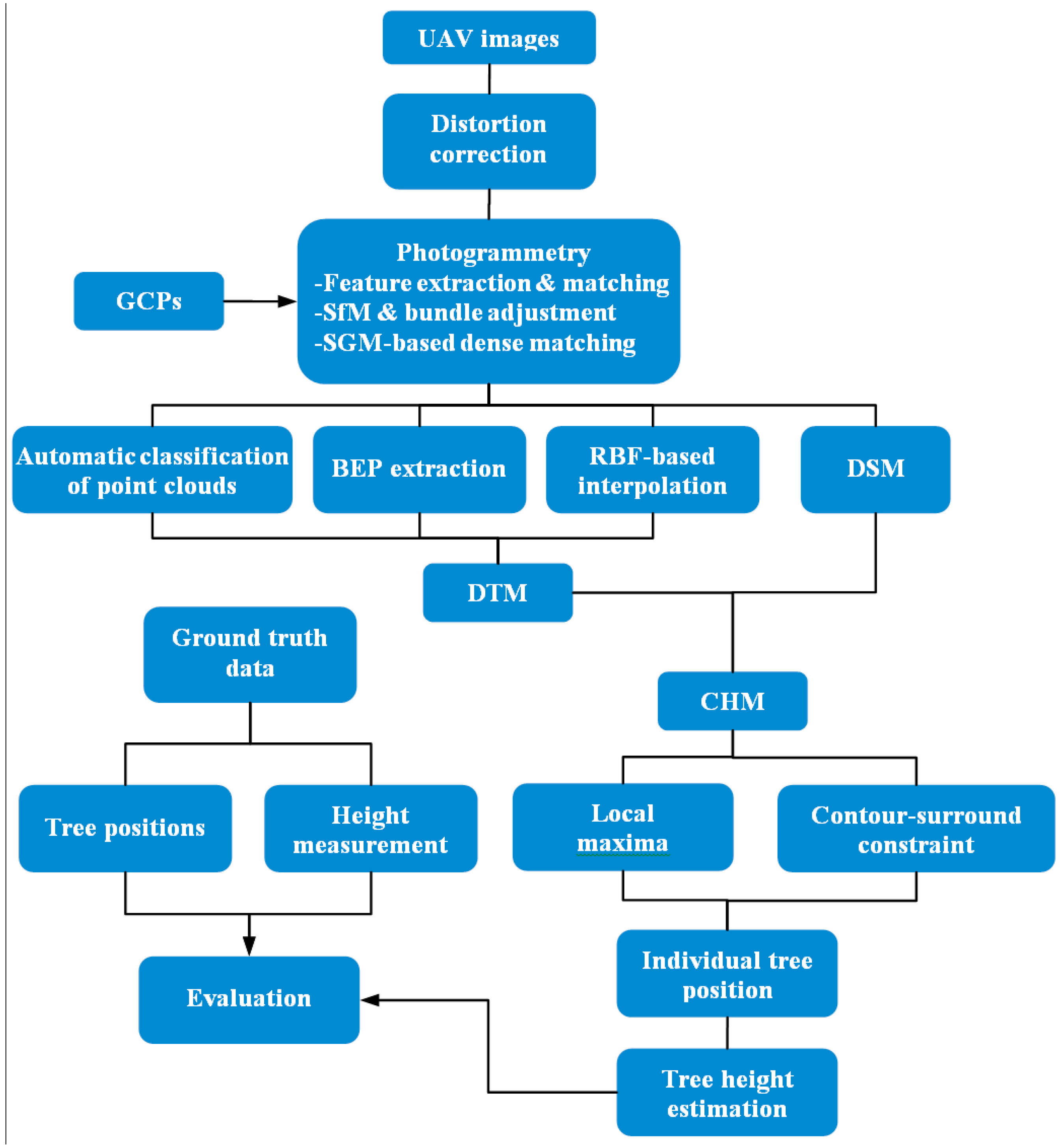
3.1. UAV-Based Photogrammetry

Low-cost UAVs (e.g., DJI Phantom quadcopters) typically carry a consumer-grade camera, thereby causing large perspective distortions and poor camera geometry [5]. Image processing started with the distortion correction of each UAV image using the camera parameters (Table 1) to minimize the systematic errors. Then, OpenCV was used to remove distortion and resample UAV images. Feature extraction and matching were performed using a sub-Harris operator coupled with the scale-invariant feature transform algorithm that was presented in a previous work [37]; this operator can obtain the evenly distributed matches among overlapping images to calculate accurate relative orientation. However, low-cost GPS and inertial measurement units shipped with DJI Phantom resulted in poor positioning and attitude accuracy, thereby posing challenges in the traditional digital photogrammetry with respect to 3D geometry generation from UAV imagery. By contrast, SfM is suitable for generating 3D geometry from the UAV imagery given the advantage of allowing 3D reconstruction from the overlapping but otherwise unordered images rather than being a prerequisite of accurate camera intrinsic and extrinsic parameters. 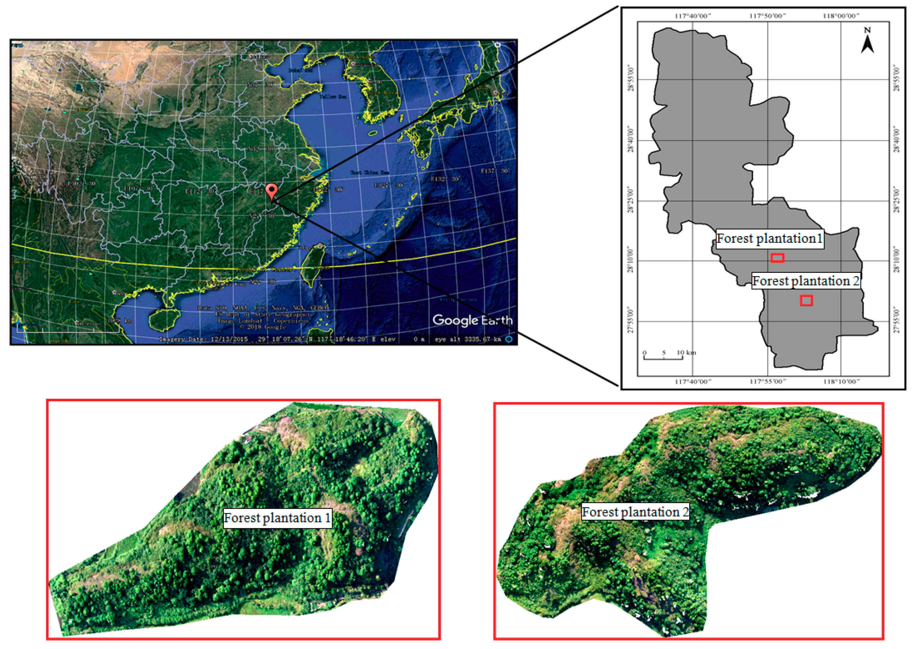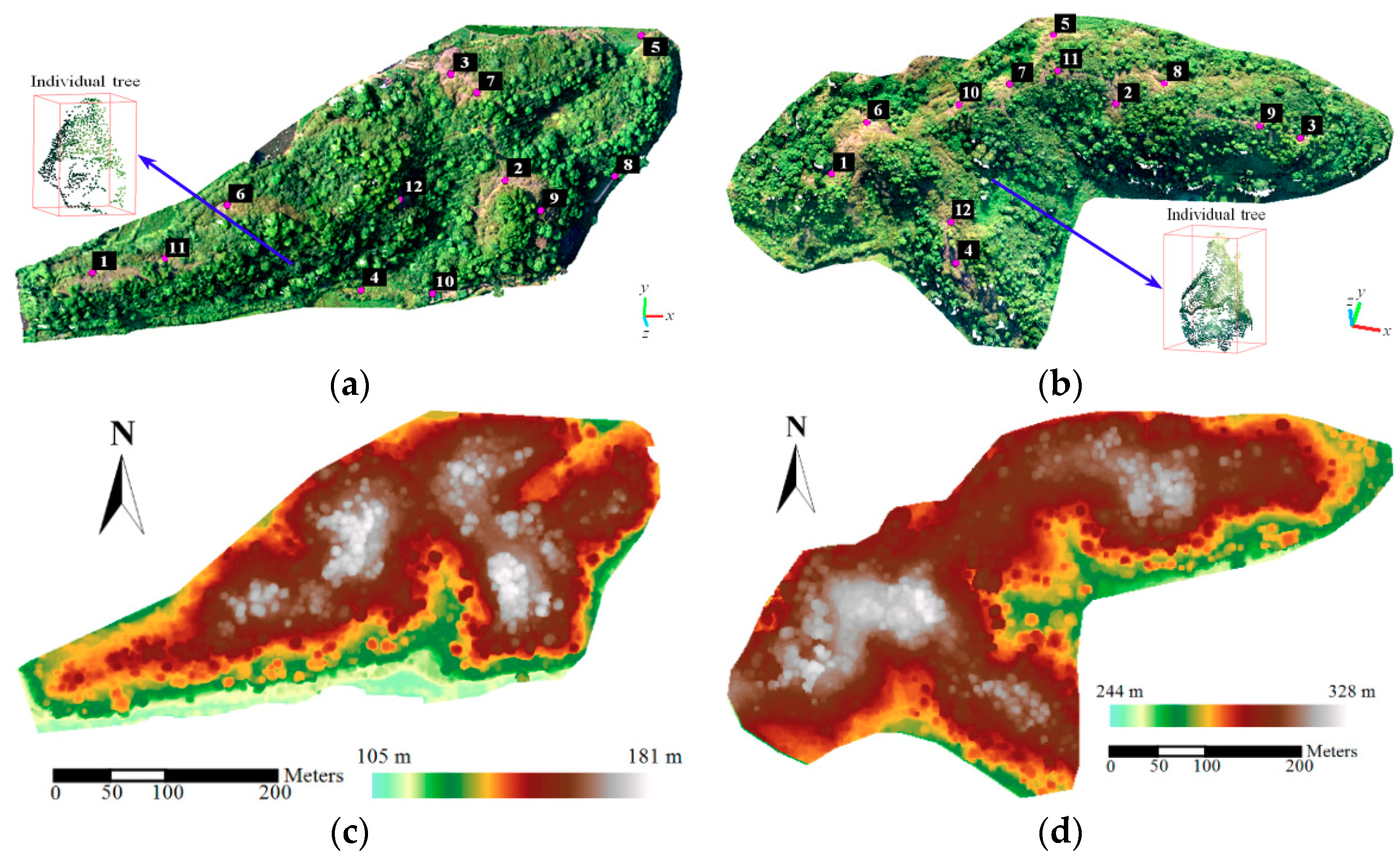Self-calibrating bundle adjustment was conducted to optimize the camera parameters, camera pose, and 3D structure using sparse bundle adjustment software package [38], and absolute orientation was performed using five evenly distributed GCPs (Nos. 1–5 in Figure 3a,b) for each of the forest plantations. In Figure 3a,b, the results of UAV-based photogrammetry through the SGM algorithm [23] consisted of $2.40\times {10}^7$ and $3.91\times {10}^7$ points for Plantations 1 and 2, respectively; these values correspond to a density of approximately 261 points/m². Thus, the DSMs for the two forest plantations were generated with a pixel size of 5 cm × 5 cm, as depicted in Figure 3c,d. The SGM enables the fine details of the tree surface to be constructed.

In Figure 3a,c, seven GCPs (Nos. 6–12) for each of the forest plantations were selected as checkpoints to evaluate the accuracy of DSMs. The residual error and Root Mean Square Error (RMSE) were calculated on the basis of the seven checkpoints and their corresponding 3D points measured using the DSM. The error statistics are summarized in

Table 2. Error statistics of checkpoints measured using DSMs. These errors are derived from differencing with checkpoints that serve as a reference. DSMs: digital surface models; RMSE: root mean square error.

Site	RMSE X (cm)	RMSE Y (cm)	RMSE Z (cm)	Total RMSE (cm)
Plantation 1	4.61	5.12	9.77	6.79
Plantation 2	5.37	5.62	8.70	6.63

. The X and Y RMSE values were approximately 5 cm, which is nearly equal to the image resolution and a relatively small horizontal error. The vertical RMSE values of the two forest plantations were less than 10 cm. Thus, these RMSE values seemed relatively satisfactory and sufficient to estimate the tree heights of the forest plantations in mountainous areas.

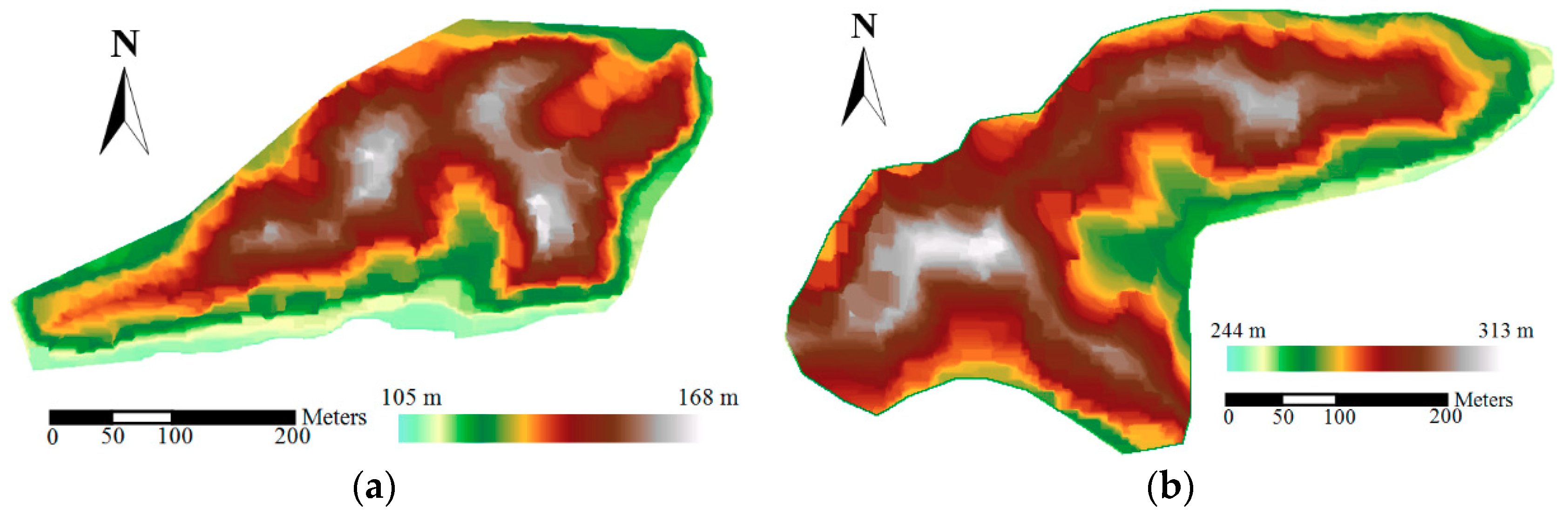
3.2. DTM Generation

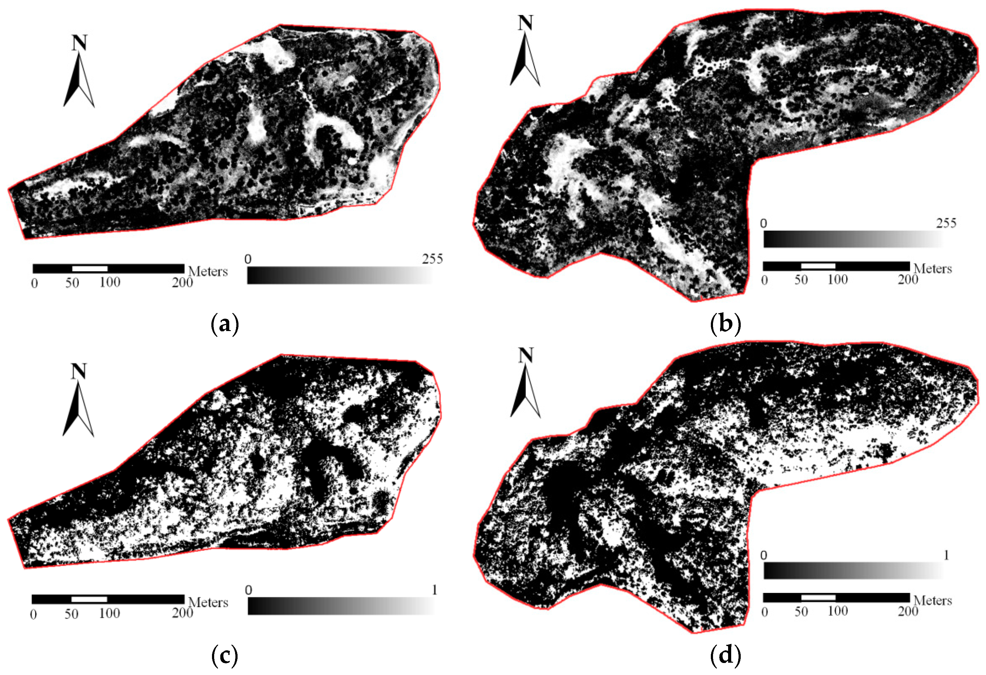
In contrast to LiDAR point clouds, UAV-based photogrammetric point clouds on the canopy of trees do not reflect the ground terrain given the lack of the ability to penetrate the upper canopy, i.e., directly separating ground points from image-derived point clouds is actually difficult. No accurate and detailed DTM is typically available in complex mountainous terrains. However, bare-earth data frequently exist in the forest plantations close to the terrain surface and allow tree heights to be modeled. To ensure that terrain fitting interpolation in the open terrain without bare-earth data (i.e., covered with abundant grass) is available, automatic classification of points and BEP extraction are jointly used in the present study to obtain ground points for DTM generation. First, initial ground points are separated from dense clouds using automatic classification with Photoscan software (version, Manufacturer, City, US State abbrev. if applicable, Country), and three parameters, namely, maximum angle, maximum distance, and cell size, are determined for Plantations 1 and 2 through multiple trials based on the most ground points that can be detected correctly. Second, 3D BEPs are extracted to replace the adjacent initial ground points, i.e., the heights of the initial ground points within 3 × 3 pixels around a BEP are replaced with the height of the BEP. BEP extraction from UAV-based photogrammetric point clouds is exploited to generate the DTM that mainly includes the following steps: (1) BEP detection and (2) denoising and 3D surface interpolation. On the basis of the gap in the spectral characteristics of RGB bands between bare land and vegetation, a bare-earth index (BEI) is created to extract 3D BEPs using inverse vegetation index and Gamma transform. The BEI is defined as follows:

$$BEI={10}^{\mathsf{\gamma }}\cdot {\left(1-GLI\right)}^{\mathsf{\gamma }},$$

(1)

where $GLI$ denotes the green leaf index calculated using $GLI=\left(2G-R-B\right)/\left(2G+R+B\right)$ [39], which is selected in accordance with favorable vegetation extraction from UAV images [40], and $R$, $G$, $B$ are the three components of RGB channels; Gamma transform is exploited to enhance contrast of BEI values for highlighting BEPs; $\mathsf{\gamma }$ denotes the Gamma value, which is set to 2.5 that is approximately estimated from the range of 0 to 255 of the BEI value in this study. The $GLI$ value is set to 0 when $GLI\le 0$, and the $BEI$ value is set to 255 when $BEI>255$. The BEI intensity maps of Plantations 1 and 2 are depicted in Figure 4a,b, but some shadow is considered bare land, i.e., shadow points may exist in 3D BEPs. An SI [32] is also used to exclude the shadow of trees from 3D BEPs. The SI is defined as follows:

$$SI=\frac{4}{\mathsf{\pi }}\cdot \arctan \left(\frac{R-G}{R+G}\right),$$

(2)

where a pixel of $SI>0.2$ is considered the shadow in this study. The value 0.2 is determined through multiple trials based on nearly all shadows that can be detected. The shadow masks of Plantations 1 and 2 are exhibited in Figure 4c,d. In Figure 4e,f, the BEPs of Plantations 1 and 2 can be then obtained from the BEI intensity maps with the corresponding shadow masks. BEPs in the vicinity of trees are prone to be related to vehicle tracks or other infrastructure or significant geological accidents (e.g., rock outcrops). The BEPs that are unrepresentative in the terrain must be removed manually.

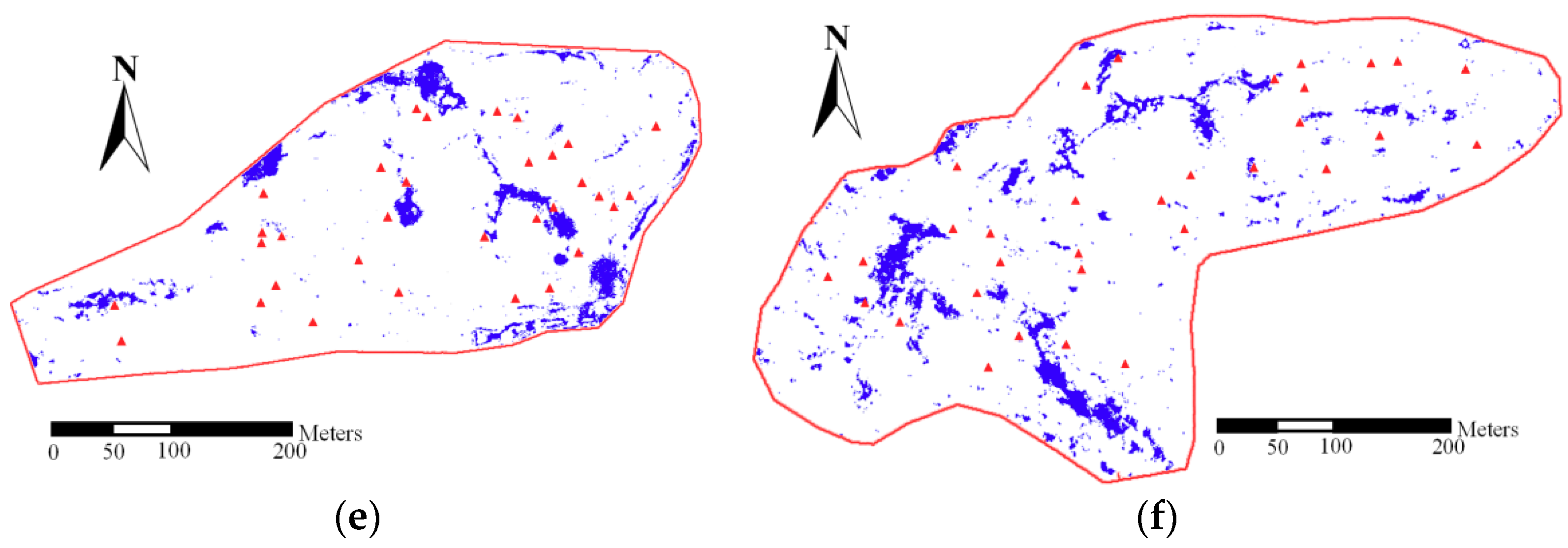
The RBF neural network performs exact interpolation [33]; thus, we use this network to interpolate the height value of each DTM grid from the 3D BEPs. In Figure 5, the RBF neural network is an artificial neural network that uses RBF as an activation function, typically including the input layer, the hidden layer of a nonlinear RBF function, and the linear output layer [41]. The RBF neural network interpolation is called exact interpolation, i.e., the output function of the RBF neural network passes exactly through all 3D BEPs. The input layer is modeled as a real vector $\mathbf{x}\in R^3$ of 3D BEP coordinates, and the output layer is a linear combination of the RBF of the inputs $\mathbf{x}$ and neuron parameters that are represented using $f:R^3\to R^1$ to generate a 1D output, i.e., a height value.

In the interpolation operator from the 3D BEPs, the vector $\mathbf{x}$ is mapped to the corresponding target output, which is the scalar function of the input vector $\mathbf{x}$ and can be computed using

$$f(\mathbf{x})={\displaystyle \sum _{i=1}^N{w}_i\varphi \left(\Vert \mathbf{x}-c_i\Vert \right)},$$

(3)

where $\Vert .\Vert$ is the norm operation and taken as the Euclidean distance here, $N$ is the number of neurons in the hidden layer, $w_i\in W$ is the weight of neuron $i$ in the linear output neuron, $c_i$ denotes the center vector of the neuron $i$, $\varphi (.)$ denotes the nonlinear function that is a multiquadratic function used in this study as follows:

$$\varphi \left(r\right)=r\sqrt{1+{\mathsf{\xi }}^2},$$

(4)

where $r$ denotes the distance between unknown and known data, and $\mathsf{\xi }$ is a smoothing factor between 0 and 1. In the training of the RBF neural network, the gradient descent algorithm is used to find the weights $W$; therefore, the RBF neural network passes through the 3D BEPs. The objective function $E$ is defined as follows:

$$E=\frac{1}{2}{\displaystyle \sum _{i=1}^n{\left(h_i-f\left(x_i\right)\right)}^2},$$

(5)

where $n$ is the number of samples, and $h_i$ is the height value of sample $i$. All weights $W$ are adjusted at each time step by moving them in the opposite direction of the gradient of $E$ until the minimum of $E$ is found, the optimization of $W$ is calculated as

$$W\left(t+1\right)=W\left(t\right)-\eta \cdot \frac{\partial E}{\partial W}=W\left(t\right)+\eta \cdot {\displaystyle \sum _{i=1}^n\left(h_i-f\left(x_i\right)\right)\varphi \left(\Vert \mathbf{x}-c_i\Vert \right)},$$

(6)

where $\eta$ is the learning rate, which can be between 0 and 1; and $t$ is the iteration count. The noisy 3D BEPs must not be traversed because the RBF is a highly oscillatory function that will not provide favorable generalization in this case [33], i.e., the RBF neural network-based interpolation performs poorly with noisy data.

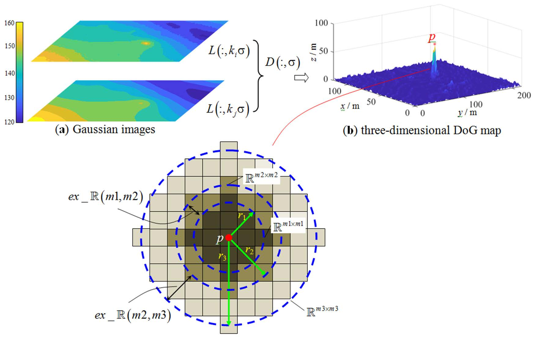
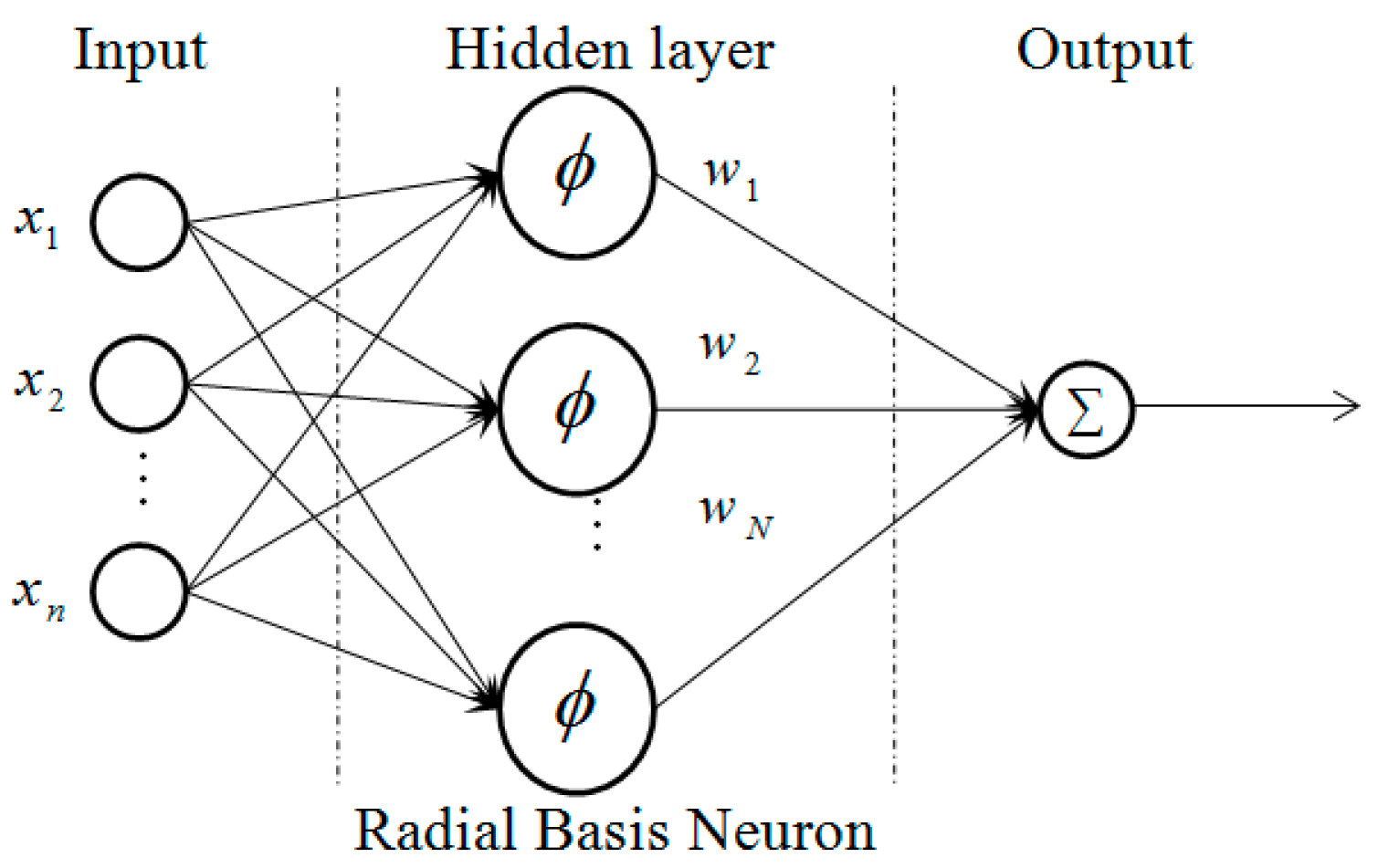
To minimize the impact of noisy data in 3D BEPs, Difference of Gaussian (DoG) operation and moving surface function are jointly applied to detect and remove the noisy data. The 3D BEPs are typically not evenly distributed in the study areas; thus, the noisy data detection is implemented in the initial DTM of a regular grid generated from the 3D BEPs adopted in the present study. The noisy data typically appear as the local maxima or minima of the height value in the initial DTM, break the continuity of the terrain surface, and form a large contrast with the surrounding height values. DoG [42] is a feature enhancement algorithm that is suitable for identifying features, considering that the height value of noisy data changes drastically and can be considered features. In Figure 6b, the noisy data $p$ are easily noticed in the DoG map. The mathematical expression $D\left(x,y,\mathsf{\sigma }\right)$ of the DoG at the pixel $\left(x,y\right)$ is calculated as

$$D\left(x,y,\mathsf{\sigma }\right)=L\left(x,y,k_i\mathsf{\sigma }\right)-L\left(x,y,k_j\mathsf{\sigma }\right),$$

(7)

where $\mathsf{\sigma }$ is the initial scale factor of the DTM and typically set as 1.6; $k_i$ and $k_j$ are the multiple factors; and $L(.)$ is the convolutional operation expressed as follows:

$$L\left(x,y,k\mathsf{\sigma }\right)=G\left(x,y,k\mathsf{\sigma }\right)\ast DEM\left(x,y\right),$$

(8)

$$G\left(x,y,k\mathsf{\sigma }\right)=\frac{1}{2\mathsf{\pi }{k}^2{\mathsf{\sigma }}^2}{e}^{-\left(x^2+y^2\right)/\left(2k^2{\mathsf{\sigma }}^2\right)},$$

(9)

where $G(.)$ denotes Gaussian filtering, and $\ast$ is the convolutional operator. A moving window with 3 × 3 pixels is used to find the local maxima or minima of height value within the DoG, which is considered a candidate $p$ for noisy data. The radius $r$ of the surrounding height values centered on candidate $p$ contaminated by noisy data can be defined as

$$r=\mathrm{INT}\left(m\cdot \mathsf{\sigma }+0.5\right),$$

(10)

where $\mathrm{INT}(.)$ denotes the integer operation, and $m$ is a multiple factor that is determined when the height values within a surrounding area do not have a significant oscillation. Specifically, in Figure 6, for example, the radius $r$ is increased at each time with $m\leftarrow m+1$, and then the surrounding regions ${ℝ}^{m1\times m1}$, ${ℝ}^{m2\times m2}$ and ${ℝ}^{m3\times m3}$ are generated with the radiuses of 2, 3, and 5 when $m$ = 1, 2, and 3, correspondingly. The extended regions $ex\_ℝ$ (i.e., closed loop areas) between the regions ${ℝ}^{m\times m}$ and ${ℝ}^{\left(m+1\right)\times \left(m+1\right)}$ displayed in Figure 6c can be determined using

$$ex\_ℝ\left(m,m+1\right)={ℝ}^{\left(m+1\right)\times \left(m+1\right)}-{ℝ}^{m\times m}\cap {ℝ}^{\left(m+1\right)\times \left(m+1\right)}.$$

(11)

We use the mean $\overline{h}$ and standard deviation $h_{\mathrm{std}}$ of the height values within the extended regions ${ℝ}^{\mathrm{ex}}$ to determine the final radius $r$ of the surrounding height values. $\overline{h}$ and $h_{\mathrm{std}}$ are computed as follows:

$$\overline{h}\left(h_i:i\in {ℝ}^{\mathrm{ex}}\right)=\frac{1}{n}{\displaystyle \sum _{i\in {ℝ}^{\mathrm{ex}}}{h}_i},$$

(12)

$$h_{\mathrm{std}}\left(h_i:i\in {ℝ}^{\mathrm{ex}}\right)=\sqrt{\frac{1}{n}{\displaystyle \sum _{i\in {ℝ}^{\mathrm{ex}}}{\left(h_i-\overline{h}\right)}^2}}.$$

(13)

The corresponding radius $r$ is considered the final radius when a newly added region ${ℝ}^{\mathrm{ex}}$ satisfies the following conditions:

$$\{\begin{array}{c}{h}_{\mathrm{std}}\left(m\right)\le h_{\mathrm{std}}\left(m-1\right)\le \dots \le h_{\mathrm{std}}\left(1\right)\\ \left|{\overline{h}}_{\mathrm{std}}\left(m\right)-{\overline{h}}_{\mathrm{std}}\left(m-1\right)\right|<\mathsf{\epsilon }\end{array},$$

(14)

where $\mathsf{\epsilon }$ is a given threshold.

The final radius$r$ can be determined using Equation (10). Candidate $p$ is regarded as a noisy point when the residual value $h_{\mathrm{residual}}^{\left(\mathrm{p}\right)}$ within the radius $r$ satisfies the following condition:

$$h_{\mathrm{residual}}^{\left(p\right)}=\left|h^{\left(p\right)}-\overline{h}\left(h_i:i\in {ℝ}^{r\times r}\right)\right|>k\cdot h_{\mathrm{std}}\left(h_i:i\in {ℝ}^{r\times r}\right),$$

(15)

where $k$ is set as 3 in this study. The moving quadratic surface-based interpolation method is used to correct the height value at Point $p$ and eliminate the contamination that occurs when interpolating the surrounding grid of the DTM. The used quadratic function is expressed as

$$z=a_0+a_{1}x+a_{2}y+a_3{x}^2+a_{4}xy+a_5{y}^2,$$

(16)

where $\left(x,y,z\right)$ denotes the coordinate of a 3D BEP; and $a_0,a_1,\dots ,a_5$ denote the six coefficients of the quadratic function, which can be solved from the 3D BEPs $\left(\left(x_i,y_i,z_i\right),i=1,2,\dots ,n\right)$ surrounding the noisy point $p$ using the least square algorithm expressed as follows:

$$X={\left(A^{\mathrm{T}}A\right)}^{-1}{A}^{\mathrm{T}}Z,$$

(17)

where $X={\left[\begin{array}{cccccc}{a}_0& a_1& a_2& a_3& a_4& a_5\end{array}\right]}^{\mathrm{T}}$, $A=\left[\begin{array}{cccccc}1& x_1& y_1& x_1^2& x_1{y}_1& y_1\\ 1& x_2& y_2& x_2^2& x_2{y}_2& y_2\\ ⋮& ⋮& ⋮& ⋮& ⋮& ⋮\\ 1& x_n& y_n& x_n^2& x_n{y}_n& y_n\end{array}\right]$, and $Z={\left[\begin{array}{cccc}{z}_1& z_2& \dots & z_n\end{array}\right]}^{\mathrm{T}}$. The correct height value of the noisy point $p$ is then derived from the quadratic surface model. The RBF neural network is (Algorithm 1) used again to perform the DTM generation after noisy data removal that can be used for achieving the height interpolation against noisy data, and the DTMs of the two forest plantations are presented in Figure 7a,b.

Algorithm 1: RBF neural network against noisy data

Parameters:$M$ and $N$ are the width and height of the DSM, respectively; $\overline{h}$ and $h_{\mathrm{std}}$ correspond to the mean and standard deviation of the height values $z$; r is the radius centered on candidate $p$; $m$ is a multiple factor; $h_{\mathrm{residual}}^{\left(\mathrm{p}\right)}$ is the residual value; and $\mathsf{\epsilon }$ is a given threshold.

Generate the DTM using the RBF neural network from the ground points.

Compute the DoG map using the DTM.

for$col=1$ to $M$ do

for $row=1$ to $N$ do

if $DoG\left(row,col\right)$ is the local maxima or minima, then

while !($h_{\mathrm{std}}\left(m\right)\le h_{\mathrm{std}}\left(m-1\right)\le \dots \le h_{\mathrm{std}}\left(1\right)$) or !($\left|{\overline{h}}_{\mathrm{std}}\left(m\right)-{\overline{h}}_{\mathrm{std}}\left(m-1\right)\right|<\mathsf{\epsilon }$)

$m\leftarrow m+1$

$r\leftarrow \mathrm{INT}\left(m\cdot \mathsf{\sigma }+0.5\right)$

$\overline{h}\left(m\right)\leftarrow \frac{1}{n}{\displaystyle \sum _{i\in {ℝ}^{\mathrm{ex}}}{h}_i}$

$h_{\mathrm{std}}\left(m\right)\leftarrow \sqrt{\frac{1}{n}{\displaystyle \sum _{i\in {ℝ}^{\mathrm{ex}}}{\left(h_i-\overline{h}\right)}^2}}$

end while

end if

$h_{\mathrm{residual}}^{\left(p\right)}\leftarrow \left|h^{\left(p\right)}-\overline{h}\left(h_i:i\in {ℝ}^{r\times r}\right)\right|$

if $h_{\mathrm{residual}}^{\left(p\right)}>k\cdot h_{\mathrm{std}}\left(h_i:i\in {ℝ}^{r\times r}\right)$ then

$p$ is regarded as a noisy point.

$p\left(z\right)$ is then derived from the fitted quadratic surface model.

Update the height value of the ground points.

end if

end for

end for

Generate the DTM using the RBF neural network from the updated ground points again.

3.3. CHM Generation

CHMs are generated by determining the DSM value in each pixel and subtracting the corresponding DTM value that can be calculated as follows:

$$CHM=DSM-DTM.$$

(18)

In Figure 7c,d, CHMs are generated using Equation (18) by finding the height value of the DSM in each pixel and subtracting the corresponding DTM value. The value of CHMs in a pixel is set to 0 when the DSM value is less than the DTM value. In addition, a 2 m-high filter is used to exclude the potential ground pixels from the canopy, i.e., the CHM generation method used does not detect understory vegetation that is less than 2 m high. The method proposed in the present study does not detect understory trees because UAV-based photogrammetry lacks the ability to penetrate dense canopies.

3.4. Tree Height Estimation

After CHM generation, the initial location of an individual tree is determined by local maxima techniques using a 1 m × 1 m moving window (i.e., 20 × 20 pixels computed by the pixel size of the DSM) to achieve accurate individual tree extraction even for overlapping trees in structurally complex forests. However, noisy pixels that are erroneously considered the vertex of an individual tree inevitably exist, i.e., multiple local maxima are frequently identified as treetops. In this study, a contour-surround constraint is used to eliminate the erroneous vertex. In particular, a vertex of the tree must be located within all closed contours generated from the CHM of an individual tree. In Figure 8, a vertex $v$ with a height value $h^{\mathrm{v}}$ satisfies the definition $v\in {ℝ}^{h_i^{\mathrm{v}}}$ (where ${ℝ}^{h_i^{\mathrm{v}}}$ denotes the closed regions surrounded by contours with the same height value $h_i^{\mathrm{v}}=h^{\mathrm{v}}-i*0.5$) and is then considered a true vertex of the individual tree; otherwise, the local maxima $v^{\prime }$ illustrated in Figure 8 is considered a pseudo vertex. The height of an individual tree is determined using the value at the vertex $v$ in the CHM.

3.5. Evaluation Criteria for Tree Height Estimation Performance

Linear regression analysis is used to model the relationship between the estimated and measured tree heights to compare the estimation of tree heights from low-cost UAV-based photogrammetric point clouds with field measurements, and the R-squared is calculated as a metric of accuracy evaluation. Paired t-tests are used to evaluate the mean of differences, and the Mean Absolute Error (MAE) [10] is also used to evaluate the residuals between individual tree heights estimated through the proposed method and the field measurements. The MAE is computed as follows:

$$MAE=\frac{1}{n}{\displaystyle \sum _{i=1}^n\left|h_i^{\mathrm{e}}-h_i^{\mathrm{m}}\right|},$$

(19)

where $n$ is the number of trees; and $h_i^{\mathrm{e}}$ and $h_i^{\mathrm{m}}$ are the estimated height and measured values, respectively.

The paired t-test of statistical analysis is commonly conducted to determine the mean differences between the estimated and measured tree heights [10,22]. The null hypothesis may be either rejected or not, i.e., determining a statistically significant difference, which is based on the paired mean different at a 0.05 significance level. The paired samples t-test can be calculated as follows:

$$t=\frac{\overline{x}}{\sqrt{s^2/n}},$$

(20)

where $\overline{x}$ is the mean of the difference between two samples, $s^2$ is the sample variance, and $n$ is the number of samples.

4. Results and Discussion

The performance of UAV photogrammetry over complex terrains plays a critical key in accurately estimating tree heights. The height accuracy (i.e., height RMSE) achieved in the present study is also compared with the results derived from other previous similar UAV photogrammetry studies conducted under complex terrain conditions. In

Table 3. Comparative table of height accuracies among UAV-based topographic surveys under complex terrain conditions. UAV: unmanned aerial vehicle; AGL: above the ground level; RMSE: root mean square error.

Study	Terrain Characteristic	Platform	AGL (m)	Height RMSE (cm)
Tonkin et al., 2014 [43]	Moraine–mound	Hexacopter	117	51.7
Long et al., 2016 [44]	Coastal	Fixed-wing	149	17
Koci et al., 2017 [45]	Gullied	Quadcopter	86/97/99	>30
Gindraux et al., 2017 [46]	Glacier	Fixed-wing	115	10–25
Gonçalves et al., 2018 [47]	Dune	Quadcopter	80/100	12
Our study	Mountainous	Quadcopter	120	9.24

, the height RMSE value of our method is superior to that of those reported by Tonkin et al. [43], Long et al. [44], Koci et al. [45], Gindraux et al. [46], and Gonçalves et al. [47] of 51.7, 17, >30, 10–25, and 12 cm, correspondingly. Our study performs better for several reasons, including sufficient image overlap, evenly distributed GCPs, and 3D reconstruction using SfM and SGM.

In the two study areas, 32 trees for each of the forest plantations are selected to evaluate the proposed method for estimating tree heights in mountainous areas. The measured and estimated height variables are summarized in

Table 4. Comparison of the measured and estimated height variables (unit: m) for the two forest plantations at the tree level. 0% (min), 25% (lower), 50% (median), 75% (upper), and 100% (max) are the quartiles that are used to extract the tree heights at the corresponding percentiles. std denotes the standard deviation of tree heights.

	Plantation 1		Plantation 2
	Measured Height	Estimated Height	Measured Height	Estimated Height
min	11.70	10.84	11.94	11.69
p25	14.68	13.19	16.83	15.39
median	16.83	17.16	19.48	19.62
p75	19.57	20.34	22.64	22.48
max	26.73	27.08	26.83	29.62
mean	17.52	17.31	19.60	19.46
std	3.85	4.20	4.31	4.84
MAE	1.45		1.73

. The tree heights of Plantations 1 and 2 range from 11.70 m to 26.73 m and from 11.94 m to 26.83 m, respectively. The measured heights of Plantations 1 and 2 are close to the estimated heights in terms of the median and mean differences of approximately equal to 0.3 m or less. The differences in standard deviation between the measured and estimated heights of Plantations 1 and 2 are approximately equal to 0.5 m.

The linear regression models depicted in Figure 9a,b exhibit a strong linear relationship between the measured and estimated tree heights in terms of $R^2=0.8345$ and $R^2=0.8238$, thereby also demonstrating the good model fit for the estimated and measured values in Plantations 1 and 2, correspondingly. The residual plots of Plantations 1 and 2 displayed in Figure 9c,d are calculated to evaluate the residuals between the measured and estimated tree heights, and the corresponding MAEs are less than 1.8 m. The MAEs close to 10% of the mean heights of the two plantations given the BEPs in the terrain with steep slopes covered by shadow are excluded, thereby reducing the accuracy of the terrain reconstruction and tree height estimation. The t-test values of Plantations 1 and 2 are calculated as 1.95 and 2.02, respectively. These values are lower than the t-table value of 2.037 (i.e., $t_{0.025/32}=2.037$). Therefore, the null hypothesis (i.e., no statistically significant difference) cannot be rejected at a 0.05 significance level. The error of tree height estimation using low-cost UAV-based photogrammetric point clouds is relatively small. Our results are superior to those of similar studies reported by Panagiotidis et al. [10] in related statistics, such as $R^2$ and MAE values, and can be considered acceptable.

To evaluate the performance of 3D BEPs in our method, we generated DTMs using the ground points obtained from automatic classification to estimate the tree heights of Plantations 1 and 2. Noncontour method for treetop identification is also compared. For a fair comparison, a DoG-coupled RBF neural network is used to generate DTMs, and the results are depicted in Figure 10a–d. Compared with the proposed method, 3D BEPs improve the accuracy of tree height estimation with stronger linear regression models and smaller residuals.

The t-test values displayed in

Table 5. Comparison of the t-test values of the three methods for the two forest plantations. ① denotes the method based on point cloud automatic classification, ② denotes the proposed method without the contour-surround constraint.

	①	②	Ours
Plantation 1	2.80	2.19	1.95
Plantation 2	2.74	2.31	2.02

indicate that the proposed method for estimating tree heights of both forest plantations is insignificantly different from the measured tree heights, whereas the two other methods are significantly different between the ground-measured and UAV photogrammetric estimated heights because their t-test values are higher than $t_{0.025/32}$. Therefore, on the basis of the t-test values of the two compared methods, the null hypothesis is rejected because both forest plantations are different at a 0.05 significance level. The proposed method performs better for both forest plantations than the two compared methods in terms of linear regression models, residuals, and t-test values. This finding may be attributed to three reasons. First, compared with the initial ground points extracted by automatic classification, the 3D BEPs obtained from the BEI maps are closer to the terrain surface, thus providing increasingly accurate ground points that help generate DTMs with higher precision. Second, the DoG-coupled RBF neural network can provide favorable generalization for DTMs from 3D ground points with noisy data. Third, contour-surround constraint is an effective solution to eliminating nontreetop maxima without reducing tree heights, whereas the DoG-coupled RBF neural network without using contour-surround constraint performs worse in terms of $R^2$ and MAE values.

5. Conclusions

The focus of this study was to estimate the tree heights of forest plantations in mountainous areas using low-cost UAV-based photogrammetric point clouds. We generated high-density 3D point clouds, and the horizontal and vertical RMSE values of DSMs were approximately equal to 5 and 10 cm, respectively. Our results showed that DTM generation using RBF neural network and 3D BEPs is suitable for producing high-quality terrain height values and CHMs. Our method exhibited a strong linear relationship and good model fit between the measured and estimated tree heights in terms of $R^2=0.8345$ and $R^2=0.8238$ for the tested Plantations 1 and 2, correspondingly. The t-test values indicated no statistically significant difference of the measured and estimated tree heights, and the error of tree height estimation using low-cost UAV-based photogrammetric point clouds was relatively small and could be considered acceptable. The overall results suggested that our method can be used as an effective alternative to field measurements for estimating tree heights of forest plantations in mountainous areas.

The proposed method still must be perfected to reconstruct the terrains with steep slopes and shadow in the southwest region of Plantation 2. Moreover, the accuracy of the DTM must be improved to estimate tree heights accurately. This study is suitable for open terrains throughout forests or plantations but not natural forests and dense mature plantations. In future studies, we will optimize the proposed method to achieve improved performance through multiple constraints, reduce low-quality 3D BEPs, and yield increasingly accurate DTMs over mountainous terrains.

References

1. Tuanmu, M.N.; Viña, A.; Bearer, S.; Xu, W.; Ouyang, Z.; Zhang, H.; Liu, J. Mapping understory vegetation using phenological characteristics derived from remotely sensed data. Remote Sens. Environ. 2010, 114, 1833–1844. [Google Scholar] [CrossRef]
2. Takahashi, M.; Shimada, M.; Tadono, T.; Watanabe, M. Calculation of trees height using PRISM-DSM. In Proceedings of the IEEE International Geoscience and Remote Sensing Symposium, Munich, Germany, 22–27 July 2012; pp. 6495–6498. [Google Scholar]
3. Lin, Y.; Holopainen, M.; Kankare, V.; Hyyppa, J. Validation of mobile laser scanning for understory tree characterization in urban forest. IEEE J. Sel. Top. Appl. Earth Obs. Remote Sens. 2014, 7, 3167–3173. [Google Scholar] [CrossRef]
4. Latifi, H.; Heurich, M.; Hartig, F.; Müller, J.; Krzystek, P.; Jehl, H.; Dech, S. Estimating over- and understorey canopy density of temperate mixed stands by airborne LiDAR data. Forestry 2015, 89, 69–81. [Google Scholar] [CrossRef] [Green Version]
5. Puliti, S.; Ørka, H.O.; Gobakken, T.; Næsset, E. Inventory of small forest areas using an unmanned aerial system. Remote Sens. 2015, 7, 9632–9654. [Google Scholar] [CrossRef]
6. Zarco-Tejada, P.J.; Diaz-Varela, R.; Angileri, V.; Loudjani, P. Tree height quantification using very high resolution imagery acquired from an unmanned aerial vehicle (UAV) and automatic 3D photo-reconstruction methods. Eur. J. Agron. 2014, 55, 89–99. [Google Scholar] [CrossRef]
7. Jing, L.; Hu, B.; Li, J.; Noland, T.; Guo, H. Automated tree crown delineation from imagery based on morphological techniques. In Proceedings of the International Symposium on Remote Sensing of Environment, Beijing, China, 22–26 April 2013; pp. 1–6. [Google Scholar]
8. Chianucci, F.; Disperati, L.; Guzzi, D.; Bianchini, D.; Nardino, V.; Lastri, C.; Rindinella, A.; Corona, P. Estimation of canopy attributes in beech forests using true colour digital images from a small fixed-wing UAV. Int. J. Appl. Earth Obs. 2016, 47, 60–68. [Google Scholar] [CrossRef] [Green Version]
9. Nilson, T. A theoretical analysis of the frequency of gaps in plant stands. Agric. Meteorol. 1971, 8, 25–38. [Google Scholar] [CrossRef]
10. Panagiotidis, D.; Abdollahnejad, A.; Surový, P.; Chiteculo, V. Determining tree height and crown diameter from high-resolution UAV imagery. Int. J. Remote Sens. 2017, 38, 2392–2410. [Google Scholar] [CrossRef]
11. Wing, B.M.; Ritchie, M.W.; Boston, K.; Cohen, W.B.; Gitelman, A.; Olsen, M.J. Prediction of understory vegetation cover with airborne lidar in an interior ponderosa pine forest. Remote Sens. Environ. 2012, 124, 730–741. [Google Scholar] [CrossRef]
12. Wallace, L.; Musk, R.; Lucieer, A. An assessment of the repeatability of automatic forest inventory metrics derived from UAV-borne laser scanning data. IEEE Trans. Geosci. Remote Sens. 2014, 52, 7160–7169. [Google Scholar] [CrossRef]
13. Wallace, L.; Watson, C.; Lucieer, A. Detecting pruning of individual stems using airborne laser scanning data captured from an unmanned aerial vehicle. Int. J. Appl. Earth Obs. Geoinf. 2014, 30, 76–85. [Google Scholar] [CrossRef]
14. Hamraz, H.; Contreras, M.A.; Zhang, J. Vertical stratification of forest canopy for segmentation of understory trees within small-footprint airborne LiDAR point clouds. ISPRS J. Photogramm. Remote Sens. 2017, 130, 385–392. [Google Scholar] [CrossRef] [Green Version]
15. Heinzel, J.; Ginzler, C. A single-tree processing framework using terrestrial laser scanning data for detecting forest regeneration. Remote Sens. 2018, 11, 60. [Google Scholar] [CrossRef]
16. Korpela, I.; Hovi, A.; Morsdorf, F. Understory trees in airborne LiDAR data—Selective mapping due to transmission losses and echo-triggering mechanisms. Remote Sens. Environ. 2012, 119, 92–104. [Google Scholar] [CrossRef]
17. Kükenbrink, D.; Schneider, F.D.; Leiterer, R.; Schaepman, M.E.; Morsdorf, F. Quantification of hidden canopy volume of airborne laser scanning data using a voxel traversal algorithm. Remote Sens. Environ. 2017, 194, 424–436. [Google Scholar] [CrossRef]
18. Lisein, J.; Pierrot-Deseilligny, M.; Bonnet, S.; Lejeune, P. A photogrammetric workflow for the creation of a forest canopy height model from small unmanned aerial system imagery. Forests 2013, 4, 922–944. [Google Scholar] [CrossRef]
19. Goodbody, T.R.H.; Coops, N.C.; Tompalski, P.; Crawford, P.; Day, K.J.K. Updating residual stem volume estimates using ALS- and UAV-acquired stereo-photogrammetric point clouds. Int. J. Remote Sens. 2017, 38, 2938–2953. [Google Scholar] [CrossRef]
20. Li, H.; Zhao, J.Y. Evaluation of the newly released worldwide AW3D30 DEM over typical landforms of China using two global DEMs and ICESat/GLAS data. IEEE J. Sel. Top. Appl. Earth Obs. Remote Sens. 2018, 11, 4430–4440. [Google Scholar] [CrossRef]
21. Selkowitz, D.J.; Green, G.; Peterson, B.; Wylie, B. A multi-sensor lidar, multi-spectral and multi-angular approach for mapping canopy height in boreal forest regions. Remote Sens. Environ. 2012, 121, 458–471. [Google Scholar] [CrossRef]
22. Birdal, A.C.; Avdan, U.; Türk, T. Estimating tree heights with images from an unmanned aerial vehicle. Geomat. Nat. Hazards Risk 2017, 8, 1144–1156. [Google Scholar] [CrossRef] [Green Version]
23. Hirschmüller, H. Stereo processing by semiglobal matching and mutual information. IEEE Trans. Pattern Anal. Mach. Intell. 2008, 30, 328–341. [Google Scholar] [CrossRef] [PubMed]
24. Turner, D.; Lucieer, A.; Watson, C. An automated technique for generating georectified mosaics from ultra-hight resolution unmanned aerial vehicle (UAV) imagery, based on structure from motion (SfM) point clouds. Remote Sens. 2012, 4, 1392–1410. [Google Scholar] [CrossRef]
25. Javernick, L.; Brasington, J.; Caruso, B. Modeling the topography of shallow braided rivers using Structure-from-Motion photogrammetry. Geomorphology 2014, 213, 166–182. [Google Scholar] [CrossRef]
26. Gonçalves, J.A.; Henriques, R. UAV photogrammetry for topographic monitoring of coastal areas. ISPRS J. Photogramm. Remote Sens. 2015, 104, 101–111. [Google Scholar] [CrossRef]
27. Cook, K.L. An evaluation of the effectiveness of low-cost UAVs and structure from motion for geomorphic change detection. Geomorphology 2017, 278, 195–208. [Google Scholar] [CrossRef]
28. Kattenborn, T.; Sperlich, M.; Bataua, K.; Koch, B. Automatic single tree detection in plantations using UAV-based photogrammetric point clouds. In Proceedings of the International Archives of the Photogrammetry, Remote Sensing and Spatial Information Sciences, ISPRS Technical Commission III Symposium, Zurich, Switzerland, 5–7 September 2014; pp. 139–144. [Google Scholar]
29. Qiu, Z.; Feng, Z.K.; Wang, M.; Li, Z.; Lu, C. Application of UAV photogrammetric system for monitoring ancient tree communities in Beijing. Forests 2018, 9, 735. [Google Scholar] [CrossRef]
30. Krause, S.; Sanders, T.G.M.; Mund, J.P.; Greve, K. UAV-based photogrammetric tree height measurement for intensive forest monitoring. Remote Sens. 2019, 11, 758. [Google Scholar] [CrossRef]
31. Marques, P.; Pádua, L.; Adão, T.; Hruška, J.; Peres, E.; Sousa, A.; Sousa, J.J. UAV-based automatic detection and monitoring of chestnut trees. Remote Sens. 2019, 11, 855. [Google Scholar] [CrossRef]
32. Sirmacek, B.; Unsalan, C. Damaged building detection in aerial images using shadow information. In Proceedings of the International Conference on Recent Advances in Space Technologies, Istanbul, Turkey, 11–13 June 2009; pp. 249–252. [Google Scholar]
33. Bullinaria, J.A. Radial basis function networks: Introduction. Neural Comput. Lect. 2004, 13, L13-2–L13-16. [Google Scholar]
34. Popescu, S.C.; Wynne, R.H.; Nelson, R.F. Measuring individual tree crown diameter with Lidar and assessing its influence on estimating forest volume and biomass. Can. J. Remote Sens. 2003, 29, 564–577. [Google Scholar] [CrossRef]
35. DJI. Phantom 4 Pro/Pro+ User Manual. 2018. Available online: https://dl.djicdn.com/downloads/phantom_4_pro/Phantom+4+Pro+Pro+Plus+User+Manual+v1.0.pdf (accessed on 5 June 2018).
36. Open Source Computer Vision Library (OpenCV). 2018. Available online: https://opencv.org/ (accessed on 5 June 2018).
37. He, H.; Chen, X.; Liu, B.; Lv, Z. A sub-Harris operator coupled with SIFT for fast images matching in low-altitude photogrammetry. Int. J. Signal Process. Image Process. Pattern Recognit. 2014, 7, 395–406. [Google Scholar] [CrossRef]
38. sba: A Generic Sparse Bundle Adjustment C/C++ Package. 2018. Available online: http://users.ics.forth.gr/~lourakis/sba/ (accessed on 5 June 2018).
39. Booth, D.T.; Cox, S.E.; Meikle, T.W.; Fitzgerald, C. The accuracy of ground-cover measurements. Rangel. Ecol. Manag. 2006, 59, 179–188. [Google Scholar] [CrossRef]
40. He, H.; Zhou, J.; Chen, M.; Chen, T.; Li, D.; Cheng, P. Building extraction from UAV images jointly using 6D-SLIC and multiscale Siamese convolutional networks. Remote Sens. 2019, 11, 1040. [Google Scholar] [CrossRef]
41. Schwenker, F.; Kestler, H.A.; Palm, G. Three learning phases for radial-basis-function networks. Neural Netw. 2001, 14, 439–458. [Google Scholar] [CrossRef]
42. Lowe, D. Object recognition from local scale-invariant features. In Proceedings of the 7th IEEE International Conference on Computer Vision, Kerkyra, Greece, 20–27 September 1999; p. 1150. [Google Scholar]
43. Tonkin, T.N.; Midgley, N.G.; Graham, D.J.; Labadz, J.C. The potential of small unmanned aircraft systems and structure-from-motion for topographic surveys: A test of emerging integrated approaches at Cwm Idwal, North Wales. Geomorphology 2014, 226, 35–43. [Google Scholar] [CrossRef] [Green Version]
44. Long, N.; Millescamps, B.; Guillot, B.; Pouget, F.; Bertin, X. Monitoring the topography of a dynamic tidal inlet using UAV imagery. Remote Sens. 2016, 8, 387. [Google Scholar] [CrossRef]
45. Koci, J.; Jarihani, B.; Leon, J.X.; Sidle, R.C.; Wilkinson, S.N.; Bartley, R. Assessment of UAV and ground-based structure from motion with multi-view stereo photogrammetry in a gullied savanna catchment. ISPRS Int. J. Geo-Inf. 2017, 6, 328. [Google Scholar] [CrossRef]
46. Gindraux, S.; Boesch, R.; Farinotti, D. Accuracy assessment of digital surface models from unmanned aerial vehicles’ imagery on glaciers. Remote Sens. 2017, 9, 186. [Google Scholar] [CrossRef]
47. Gonçalves, G.R.; Pérez, J.A.; Duarte, J. Accuracy and effectiveness of low cost UASs and open source photogrammetric software for foredunes mapping. Int. J. Remote Sens. 2018, 39, 5059–5077. [Google Scholar] [CrossRef]
Figure 1. Two forest plantations selected from the study site in Shangrao, Southern China.
Remotesensing 11 01271 g001
Figure 2. Workflow of the tree height estimation of forest plantation in mountainous areas using UAV-based photogrammetry. UAV: unmanned aerial vehicle.
Remotesensing 11 01271 g002
Figure 3. Photogrammetric point clouds and DSMs of the two forest plantations. (a,b) are the photogrammetric point clouds in 3D space with the true color of Plantations 1 and 2, respectively. (c,d) are the DSMs of Plantations 1 and 2, correspondingly. Twelve GCPs are labeled for each of the forest plantations, and the point clouds of individual trees are enlarged to be exhibited in (a,b). DSMs: digital surface models; GCPs: ground control points.
Remotesensing 11 01271 g003
Figure 4. BEI maps, SI maps, and BEPs of the two forest plantations. (a,b) are the BEI intensity maps of Plantations 1 and 2, respectively. (c,d) are the shadow masks of Plantations 1 and 2, correspondingly. The BEPs of Plantations 1 and 2 are marked in (e,f), respectively. Red triangles denote the sample trees, red line denotes the boundary of each plot, and the blue pixels denote the BEPs. BEI: bare-earth index; SI: shadow index; BEPs: bare-earth points.
Remotesensing 11 01271 g004aRemotesensing 11 01271 g004b
Figure 5. Architecture of the RBF neural network. RBF: radial basis function.
Remotesensing 11 01271 g005
Figure 6. Example of the DoG operation and noisy point detection. DoG: difference of Gaussian.
Remotesensing 11 01271 g006
Figure 7. DTMs and CHMs of the two forest plantations. (a,b) are the DTMs of Plantations 1 and 2, respectively. (c,d) are the CHMs of Plantations 1 and 2, correspondingly. DTMs: digital terrain models; CHMs: canopy height models.
Remotesensing 11 01271 g007aRemotesensing 11 01271 g007b
Figure 8. Contour-surround constraint for pseudo vertex removal. (ac) correspond to an individual tree, the CHM of the individual tree, and the contour of the CHM. Red and blue triangles denote true and pseudo vertices, respectively. CHMs: canopy height model.
Remotesensing 11 01271 g008
Figure 9. Linear regression models and residual plots of the ground-measured and UAV photogrammetric estimated heights. (a,b) are the linear regression models of Plantations 1 and 2, respectively. (c,d) are the residual plots of Plantations 1 and 2, correspondingly.
Remotesensing 11 01271 g009
Figure 10. Comparisons of linear regression models and residual plots obtained from the two other methods. (a,c) are the linear regression models through the method based on point cloud automatic classification of Plantations 1 and 2, respectively; the corresponding residual plots are (b,d). (e,g) are the linear regression models through the proposed method without the contour-surround constraint of Plantations 1 and 2, correspondingly; the corresponding residual plots are (f,h).
Remotesensing 11 01271 g010aRemotesensing 11 01271 g010b