Double-Branch Multi-Attention Mechanism Network for Hyperspectral Image Classification

Abstract

Recently, Hyperspectral Image (HSI) classification has gradually been getting attention from more and more researchers. HSI has abundant spectral and spatial information; thus, how to fuse these two types of information is still a problem worth studying. In this paper, to extract spectral and spatial feature, we propose a Double-Branch Multi-Attention mechanism network (DBMA) for HSI classification. This network has two branches to extract spectral and spatial feature respectively which can reduce the interference between the two types of feature. Furthermore, with respect to the different characteristics of these two branches, two types of attention mechanism are applied in the two branches respectively, which ensures to extract more discriminative spectral and spatial feature. The extracted features are then fused for classification. A lot of experiment results on three hyperspectral datasets shows that the proposed method performs better than the state-of-the-art method.

1. Introduction

Recently, remote sensing image has been studied in more and more areas, including image registration [1,2,3], change detection [4,5], object detection [6] and so on. As is known to all, Hyperspectral Imaging (HSI) is a special type of remote sensing image which has abundant spectral and spatial information [7], and has been studied in many fields, including forest vegetation cover monitoring [8], classification of land-use [9,10], change area detection [11], anomaly detection [12] and environmental protection [13].

In HSI, supervised classification is the most studied task. However, the high-dimensional nature of the spectral channel can bring with it the ’curse of dimensionality’, which makes conventional techniques inefficient. How to extract the most discriminative feature from the high dimensionality of the spectral channel is the key in HSI classification. Therefore, traditional HSI classification methods usually contain two steps, e.g., feature engineering and classifier classification. There are two mainstreams in feature engineering, one is feature selection and the other is feature extraction. Feature selection aims to pick up several spectral channel to reduce dimensionality and feature extraction refers to using some nonlinear mapping function to transform the original spectral domain to a lower dimensional space. After feature engineering, the selected feature or extracted feature will be fed to general-purpose classifiers for classification.

In the early stage, researchers focused on spectral-based methods and without considering the spatial information. However, HSI has local consistency, so some researchers took spatial information into consideration and had performed better. Gabor feature [14] and differential morphological profile (DMP) [15] feature are two types of low-level feature which could represent the shape information of the HSI and could also lead to satisfactory classification results. In [16], Paheding et al. used multiscale spatial texture features for HSI classification. However, The HSI usually contains various types and levels features, so it is impossible to describe all types of objects by setting empirical parameters. One method may perform well on a dataset while performs worse on another dataset.

Deep Learning (DL) has shown extremely powerful ability to extract hierarchical and nonlinear features, which are very useful for classification. So far, many works based on DL have been done in the community of HSI classification. For example, Chen et al. [17] used stacked autoencoder (SAE) to extract spectral and spatial features and use logistic regression to get classification result. Similarly, they used a Restricted Boltzmann Machine (RBM) and deep belief network (DBN) in [18] for classification. Tao et al. [19] used two sparse stacked auto-encoder to learn the spatial and spectral features of the HSI separately, then he stacked the spatial and spectral features and fed them into a liner SVM for classification. Ma et al. [20] used a spatial updated deep autoencoder to extract both spatial and spectral information with a single deep network, and utilized an improved collaborative representation in feature space for classification. Zhang et al. [21] utilized a recursive autoencoder to learn spatial and spectral information and adopted a weighting scheme to fuse the spatial information. In [22], Paheding et al. proposed a Progressively Expanded Neural Network (PEN Net), which is a novel neural network.

The input of the aforementioned methods is one dimensional, and they utilized the spatial feature but destroyed the initial spatial structure. With the emergence of the convolutional neural network (CNN), some new methods have also been introduced. CNN can extract the spatial information without destroying the original spatial structure. For example, Hu et al. [23] employed deep CNN for HSI classification. Chen et al. [24] proposed a novel 3D-CNN model combined with regularization to extract spectral-spatial features for classification. The obtained results reveal that 3D-CNN perform better than 1D-CNN and 2D-CNN. Mercedes E. Paoletti et al. [25] proposed the deep pyramidal residual network to extract multi-scale spatial feature for classification. Recently, some new training methods also have emerged in the literature, including active learning [26], self-pace learning [27], semi-supervised learning [28] and generative adversarial network (GAN) [29]. Furthermore, some superpixels based methods also play an important role in HSI classification [30,31]. In [32], Jiang et al. studied the influence of label noise on the HSI classification problem and proposed a random label propagation algorithm (RLPA) which is used to cleanse the label noise.

1.1. Motivation

Inspired by the residual network [33], Zhong et al. [34] proposed a Spectral–Spatial Residual Network (SSRN) which contains spectral residual block and spatial residual block to extract spectral features and spatial features sequentially. SSRN has achieved the state-of-the-art performance in HSI classification problem. Based on SSRN and DenseNet [35], Wang et al. [36] proposed a fast densely connected spectral–spatial convolution network (FDSSC) for HSI classification and has achieved better performance while reducing the training time.

Although SSRN and FDSSC have achieved the highest classification accuracy, there are still some problems need to be solved. The biggest problem is that the two frameworks firstly extracts spectral features then extracts spatial features. In the procedure of extracting spatial features, the extracted spectral features may be destroyed because the spectral features and spatial features are in different domain.

More recently, Fang et al. [37] proposed a network using 3-D CNN with spectral-wise attention mechanism (MSDN-SA) which applied spectral-wise attention mechanism in a densely connected 3D convolution network. However, it only considers the spectral-wise attention while not considering the spatial-wise attention.

Recently, an intuitive and effective attention module named Convolutional Block Attention Module (CBAM) was proposed in [38], which sequentially applies channel attention mechanism and spatial attention mechanism in the network to adaptively refine the feature map, which results in improvements in classification performance.

Inspired by the CBAM and to solve the problem of SSRN and FDSSC, we propose the double-branch multi-attention mechanism network for HSI classification. The framework consists of two parallel branches, i.e., spectral branch and spatial branch. To extract more discriminative features, in the spectral branch and spatial branch we apply channel-wise attention and spatial-wise attention separately. After the two branches extract corresponding features, we fuse them by a concatenation operation to get the spectral-spatial feature. Finally, the softmax classifier are added to get the last classification result.

1.2. Contribution

To be summarized, our main contributions can be listed as follows:

• We propose a densely connected 3DCNN-based Double-Branch Multi-Attention mechanism network (DBMA). This network has two branches to extract spectral and spatial features separately which can reduce the interference between the two types of features. The extracted spectral and spatial features are fused for classification.
• We apply both the channel-wise attention and spatial-wise attention in the HSI classification problem. The channel-wise attention is aiming to emphasize informative spectral features while suppress less useful spectral features, while the spatial attention is aimed at focusing on the most informative ares in the input patches.
• Compared with other recently proposed methods, the proposed network achieves the best classification accuracy. Furthermore, the training time and test time of our proposed network are also less than the two compared deep-learning algorithm, which indicates the superiority of our method.

The rest of this paper is organized as follows: Section 2 illustrates the related work. Section 3 presents a detailed description of the proposed classification method. The experiment results and analysis are provided in Section 4. Finally, Section 5 concludes the whole paper and briefly introduce our future research.

2. Related Work

In this section, we will briefly introduce some basic knowledge and related work, including cube-based HSI classification framework, residual connection and densely connection, FDSSC and attention mechnasim.

2.1. Cube-Based HSI Classification Framework

Traditional pixel-based classification architecture only uses spectral information for classification while cube-based architecture uses both spectral and spatial information. Given an HSI dataset with size of $X\in {\mathbb{R}}^{w\times h\times d}$, There are total $w\times h$ pixels in the image, however, only N pixels has corresponding labels. Firstly, we random split the pixels with their labels into three sets, i.e., training set, validation set and test set. Then, we extract the 3D cube as the input of the network. Different from a pixel-based architecture which directly uses the pixel as input to train network for classification, cube-based framework uses 3D structure of HSI for classification. The reason using cube-based framework is that the spatial information is also important for classification.

2.2. Residual Connection and Densely Connection

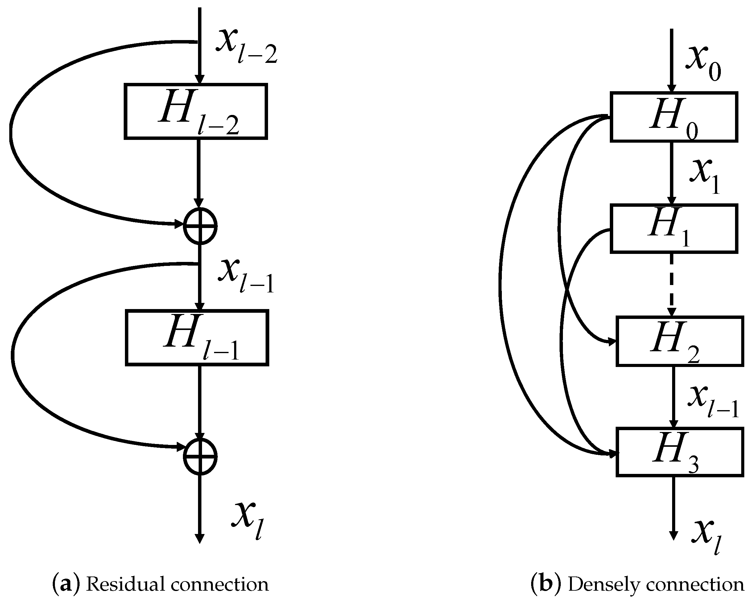
Residual connection was first proposed in [33]. In principle, a residual connection adds a skip connection in the basic of tradition CNN model. As is shown in Figure 1a, H is the abbreviation of hidden block and represents several convolutional layers with activation layers and BatchNorm layers. ResNet allows input information to be passed directly to subsequent layers. The skip connection can be seen as an identity mapping. In ResNet, the output of the l-th block can be computed as:

$$x_l=H_l\left(x_{l-1}\right)+x_{l-1}$$

(1)

Through the residual connection, the original function $F\left(x\right)$ can be transformed to $H\left(x\right)+x$. In addition the $H\left(x\right)$ is easy to learn than $F\left(x\right)$. Therefore, ResNet can achieve better result than traditional CNN models. Furthermore, ResNet wouldn’t bring extra parameters but can speed up the training process.

Based on residual connection, Gao et al. [35] proposed the concept of densely connection and DenseNet. In DenseNet, any hidden block has path to any previous block and back block. Differing from the residual connection, which combines features through summation, dense connectivity combines features by concatenating them. In DenseNet, all previous feature maps of lblocks can be used to compute the output of the l-th block:

$$x_l=H_l[x_0,x_1,\dots ,x_{l-1}]$$

(2)

where $x_0,\dots ,x_{l-1}$ is the feature maps of the previous blocks. $H_l(·)$ consists of batch normalization (BN), activation layers and convolution layers. In DenseNet, as is shown in Figure 1b, each block has been linked to each previous block and back block. Note that if each function $H_l$ produces k feature maps, the $(l+1)th$ layer will have $k_0+k\times (l-1)$ input features, where $k_0$ is the number of channels in the input layer, while the output will still be k feature maps.

2.3. Fast Dense Spectral–Spatial Convolution Network (FDSSC)

Based on residual connection, Zhong et al. [34] proposed a Spectral–Spatial Residual Network (SSRN) which contains spectral residual block and spatial residual block to extract spectral features and spatial features sequentially. Inspired by SSRN and DenseNet, Wang et al. [36] proposed the FDDSC network for HSI classification which achieved better performance while reduced the training time. In this part, we will introduce FDSSC in detail.

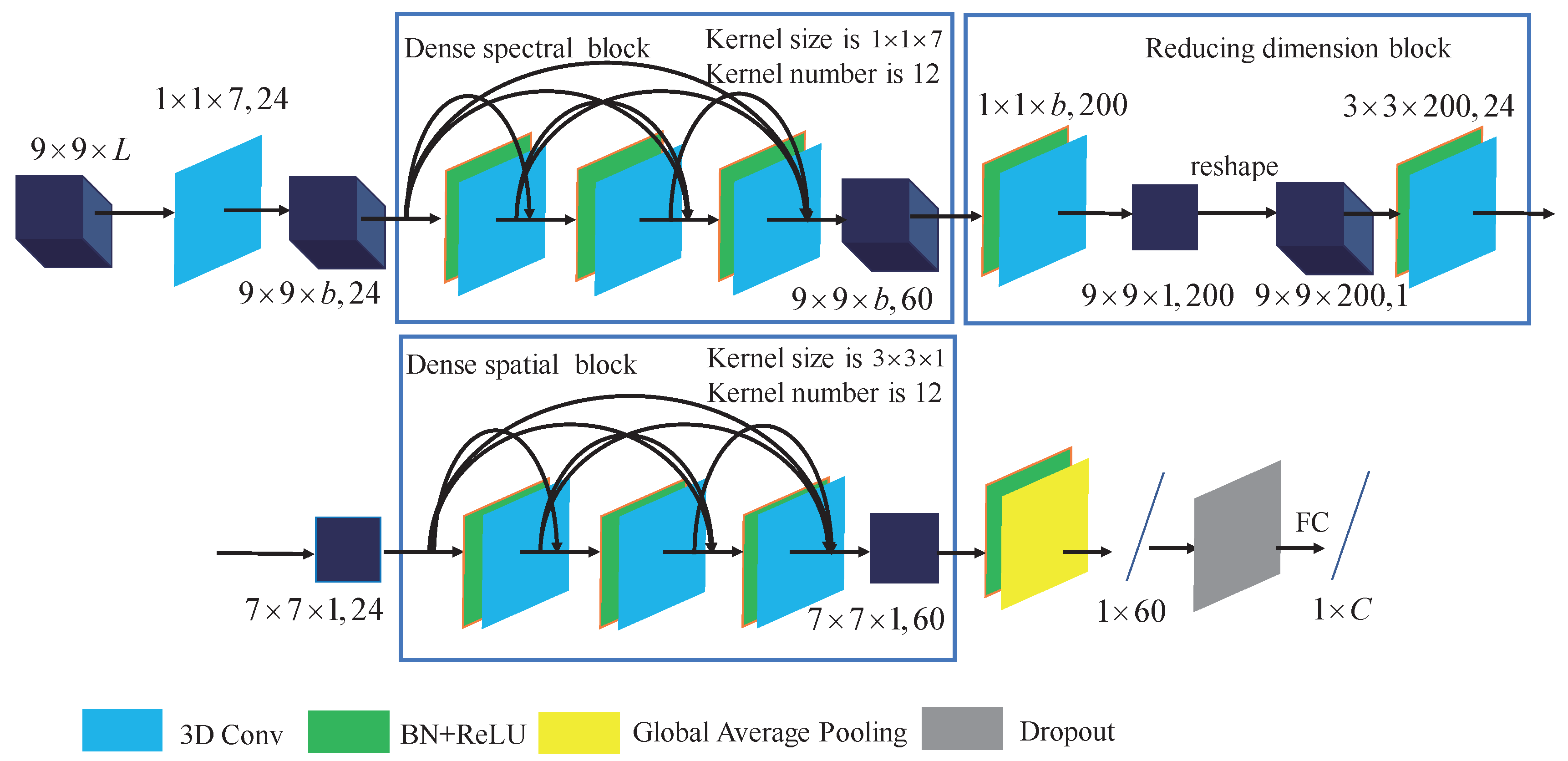
As illustrated in [36], the structure of FDSSC is shown in Figure 2. FDSSC consists of a dense spectral block, a reducing dimension block and a dense spatial block. The input patch of FDSSC is set to $9\times 9\times L$. The dense spectral block aims to extract spectral feature using densely connected 3D convolution and the kernel size is set to $1\times 1\times 7$. The $1\times 1\times d$ ($d>1$) convolution operation does not extract any spatial features because the kernel size of spatial dimension is set to 1. Therefore, a kernel size of $1\times 1\times 7$ extracts the spectral features and retains the spatial features. Through the dense spectral block, we get spectral feature with size of $(9\times 9\times b,60)$. 60 refers to the number of feature maps.

The reducing dimension block aims to reduce the dimension of feature maps and the number of parameters to be trained. In reducing dimension block, the padding method of 3D convolution is set to ’valid’ to decrease the size of feature maps. After learning the spectral features, we get 60 feature maps with size of $9\times 9\times b$. Then, the 3D convolution layer with kernel size of $1\times 1\times b$ is used to get 200 feature maps with size of $9\times 9\times 1$. After that, the feature maps are reshaped to get 1 feature map with size of $9\times 9\times 200$. To further reduce the dimension of feature maps’ size, the convolution layer with kernel size of $3\times 3\times 200$ transformed the feature maps to get feature maps with size of $(7\times 7\times 1,24)$.

Then, the dense spatial block is used to extract spatial features. The kernel size in the dense spatial block is set to $3\times 3\times 1$. A kernel with size of $a\times a\times 1$ ($a>1$) learns the spatial features while not learning any spectral features.

After the dense spatial block, we get feature with size of $(7\times 7\times 1,60)$. Then, the global average pooling layer is employed to get a feature vector with length of 60. The global average pooling layer can be seen as a special case of pooling layer which can aggregate information and reduce parameters. The feature vector is feed to softmax classifier for classification result.

2.4. Attention Mechanism

Inspired by the human perception process [39], the attention mechanism has been applied in the image categorization [40], and were later shown to yield significant improvements for Visual Question Answering (VQA) and captioning [41,42,43]. As is known to all, the importance of every spectral channel and the area of the input patch is different while extracting features. In addition, the attention mechanism can focus on the most informative part and decrease other region’s weight, which is believed to be similar to the human eye’s attention mechanism. In CBAM [38], the network has two attention module, i.e., channel attention module and spatial attention module which focus on informative channel and informative area respectively. Later, we will introduce the two modules in detail.

2.4.1. Channel-Wise Attention Module

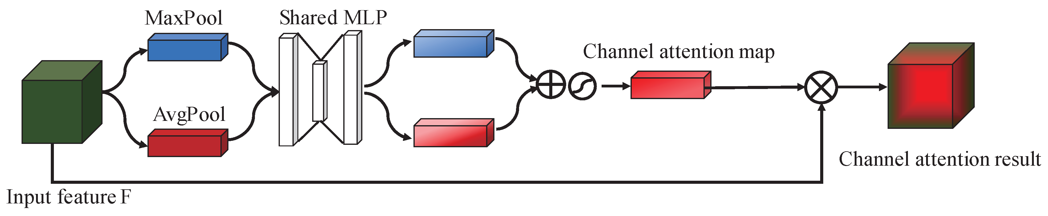
The channel-wise attention module mainly refines the feature maps’ weight in the channel-wise. Each channel of the feature map can be seen as a feature detector, and channel attention focuses on the meaningful channel and decrease the meaningless channel’s value to a certain degree.

As is shown in Figure 3, a MaxPooling layer and an AvgPooling layer are used to aggregate spatial information, the two pooling operations can be seen as two different spatial descriptors: $F_{avg}^c$ and $F_{max}^c$, which denote average-pooled features and max-pooled features respectively. Note that the output features are a one-dimensional vector and the length of the vector is the same as the number of the input features. Then the two types of features are feed forwarded to a shared network to produce the channel attention map. The shared network is composed of a 3-layer perceptron (MLP) with one hidden layer. The hidden layer has $C/L$ units, which is used to reduce the training numbers and generate more nonlinear mapping, where L is the reduction ratio and C is the channel numbers. Then the output feature vectors are merged using element-wise summation. Through the sigmoid function, the channel attention map is obtained. The channel attention map is a vector of which the length is the same as the number of input feature maps and the value is in range of (0,1). The bigger the value is, the more important the corresponding channel is. Then the channel attention map is multiplied with the input feature to get the channel-refined feature. The procedure of generating mapping function can be computed as:

$$M_c\left(F\right)=\sigma (MLP\left(AvgPool\left(F\right)\right)+MLP\left(MaxPool\left(F\right)\right))=\sigma (W_1\left(W_0\left(F_{avg}^c\right)\right)+W_1\left(W_0\left(F_{max}^c\right)\right))$$

(3)

where $\sigma$ is the sigmoid function, $W_0\in C/L\times C$ and $W_1\in C\times C/L$. It has to be noted that the MLP weights, $W_0$ and $W_1$ are shared for both inputs.

2.4.2. Spatial-Wise Attention Module

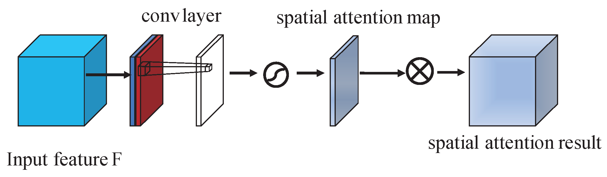
In contrast to the channel-wise attention, the spatial-wise attention focuses on the informative region of the spatial dimension. As is shown in Figure 4, similar to the channel-wise attention module, two types of pooling operations are used to generate different feature descriptors: $F_{avg}^s\in {\mathbb{R}}^{1\times H\times W}$ and $F_{max}^s\in {\mathbb{R}}^{1\times H\times W}$. In contrast with the channel-wise attention module, the pooling operation in the spatial-wise attention module is along the channel axis. Then, the output feature descriptors are fused by concatenation operation. Then a convolution layer is applied to the concatenated feature. After the convolution layer, we can get the spatial attention map. Then, the input feature is multiplied with the spatial attention map to get spatial-refined feature maps which focus on the most informative region. To be summarized, the spatial attention map is computed as:

$$M_s\left(F\right)=\sigma \left(f^{N\times N}\left([AvgPool\left(F\right);MaxPool\left(F\right)]\right)\right)=\sigma \left(f^{N\times N}\left([F_{avg}^s;F_{max}^s]\right)\right)$$

(4)

where $\sigma$ denotes the activation function and we choose the sigmoid function here, $f^{N\times N}$ represents a convolution operation with the filter size of $N\times N$.

3. Methodology

FDSSC has achieved a very high performance in HSI classification, however, it firstly extracts spectral feature then extracts spatial feature. It means that the firstly extracted spectral features may be influenced in the process of extracting the spatial features because the two types of features are in different domain. In contrast to FDSSC, in our framework, the spectral feature and spatial feature are extracted in two parallel branches and fused for classification.

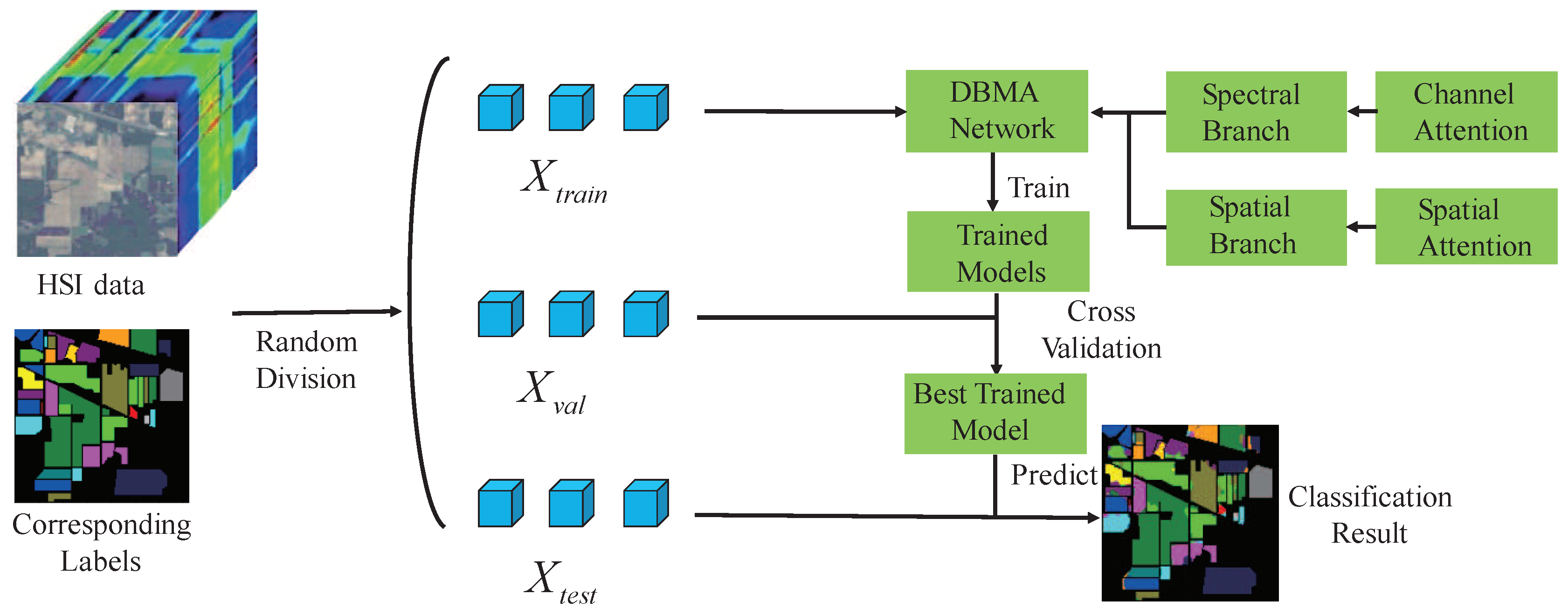
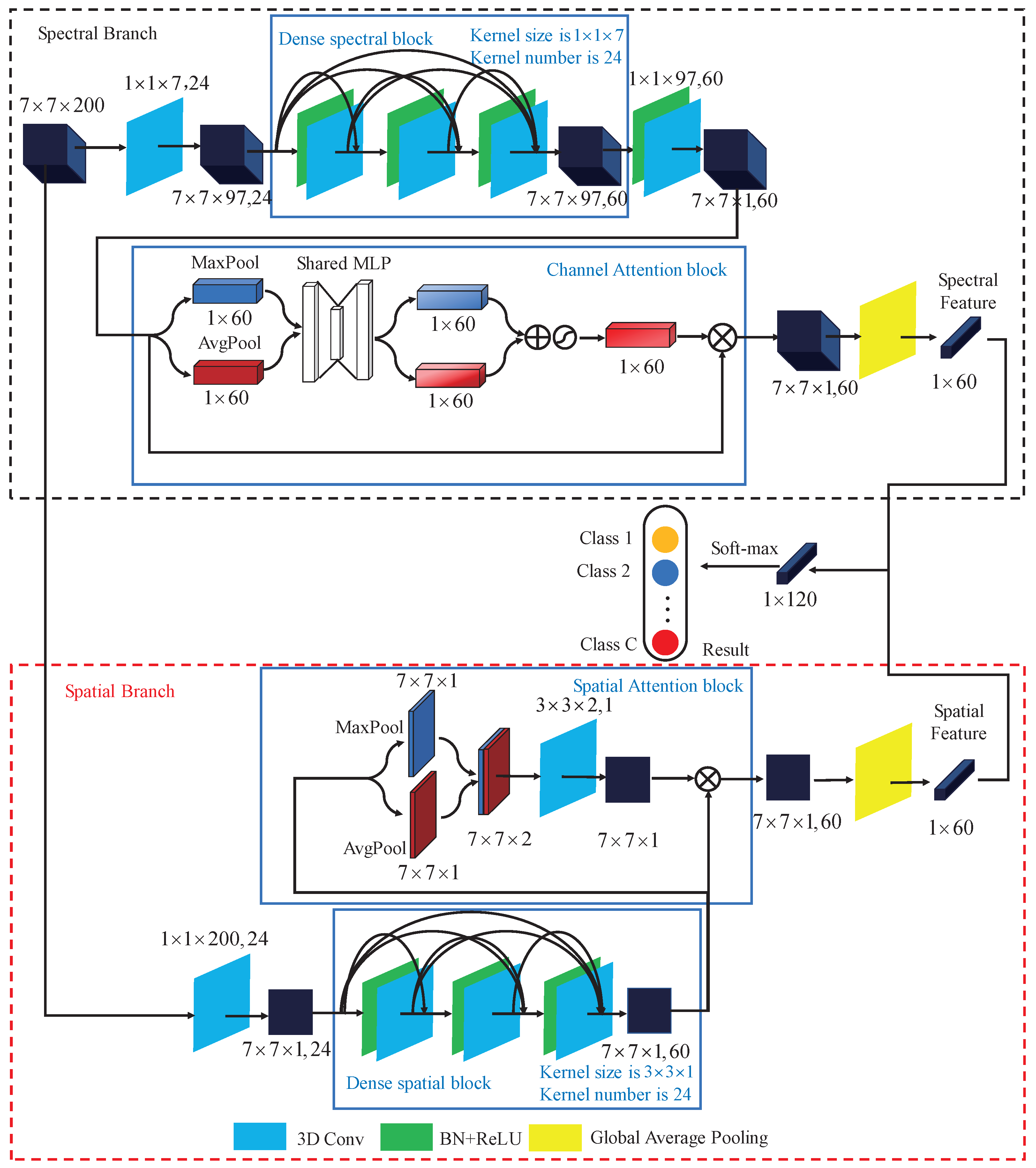
Figure 5 illustrates the whole framework of our method. Firstly, given a hyperspectral image with $H\times W\times L$ size, we extract the $7\times 7$ neighborhoods of the center pixel together with its corresponding category label as samples. In contrast to FDSSC using $9\times 9$ neighborhoods as input, we use a smaller input size which can reduce the training time. Then, we divide the samples into 3 sets, i.e., training set $X_{train}$, validation set $X_{val}$ and testing set $X_{test}$. The training set is used for training model for many epochs, validation set is used for evaluating the classification accuracy and to pick up the network with the highest classification accuracy. Finally, the testing set is used for testing the trained model and the effectiveness of the proposed method. As can be seen in Figure 5, our network has two branches, i.e., Spectral Branch with Channel Attention and Spatial Branch with Spatial Attention. As can be seen in Figure 6, for convenience, the top branch is called Spectral Branch while the bottom one is called Spatial Branch. Next, we will introduce the two branches.

3.1. Spectral Branch with Channel Attention

We take Indian Pines dataset for example and the input patch size is set to $7\times 7\times 200$. Spectral Branch consists of a dense spectral block and a channel attention block. First of all, 3D convolutional with kernel size of $1\times 1\times 7$ is used. In the first convolutional operation, we use ’valid’ padding method and the stride is set to (1,1,2), which is used to reduce the number of spectral channels to a certain degree. After the first convolutional layer, feature maps’ with shape of ($7\times 7\times 97$, 24) are obtained. Then, the dense spectral block which consists of 3 convolutional layers with batch normalization layers is used to extract spectral feature. In the dense spectral block, as the existence of concatenation, we set the stride to (1,1,1) to maintain the feature maps’ size. After dense spectral block, spectral feature with size of ($7\times 7\times 1$, 60) is obtained. However, the importance of the 60 channels is different. To focus on which is important and obtain more discriminative spectral feature, channel attention block as illustrated in Section 2.4.1 is applied. After channel attention block, the important channel will be highlighted while the less important channel will be suppressed. Finally the Global Average Pooling layer is employed to get the spectral feature with size of $1\times 60$. Details of the layers of the Spectral Branch are described in

Table 1. Network structure of Spectral Branch.

Layer Name	Kernel Size	Output Size
Input	-	($7\times 7\times 200$)
Conv	($1\times 1\times 7$)	($7\times 7\times 97,24$)
BN-Relu-Conv	($1\times 1\times 7$)	($7\times 7\times 97,24$)
Concatenate	-	($7\times 7\times 97,24$)
BN-Relu-Conv	($1\times 1\times 7$)	($7\times 7\times 97,24$)
Concatenate	-	($7\times 7\times 97,24$)
BN-Relu-Conv	($1\times 1\times 7$)	($7\times 7\times 97,24$)
Concatenate	-	($7\times 7\times 97,24$)
BN-Relu-Conv	($1\times 1\times 97$)	($7\times 7\times 1,60$)
AveragePooling/maxpooling	($7\times 7\times 1$)	($1\times 1\times 1,60$)
Add	-	($1\times 1\times 1,60$)
FC	30	30
FC-sigmoid	60	60
Multiply	-	($7\times 7\times 1,60$)
GlobalAveragePooling	-	($1\times 60$)

.

3.2. Spatial Branch with Spatial Attention

Spatial Branch consists of a dense spatial block and a spatial attention block. First of all, 3D convolutional with kernel size of $1\times 1\times 200$ is used to reduce the number of spectral channels. After the first convolution layer, feature maps with shape of ($7\times 7\times 1$, 24) will be obtained. The number of spectral channel decreases from 200 to 1, which will reduce the number of training parameters and prevent overfitting. Then the dense spatial block consists of 3 convolutional layers together with batch normalization layers is used to extract spatial feature. After dense spatial block, spatial feature with size of ($7\times 7\times 1$, 60) is obtained. The dense spatial block aims to extract spatial feature, however, the importance of different position of the input patch is different. To focus on ’where’ is an informative part and get more discriminative spatial feature, the spatial attention block in Section 2.4.2 is used. After Spatial attention block, the features of areas where is more important will be highlighted while the features of areas where is less important will be suppressed. Then the Global Average Pooling layer is employed to get the spatial feature with size of $1\times 60$. Details of the layers of the Spatial Branch are described in

Table 2. Network structure of Spatial Branch.

Layer Name	Kernel Size	Output Size
Input	-	($7\times 7\times 200$)
Conv	($1\times 1\times 200$)	($7\times 7\times 1,24$)
BN-Relu-Conv	($3\times 3\times 1$)	($7\times 7\times 1,24$)
Concatenate	-	($7\times 7\times 1,24$)
BN-Relu-Conv	($3\times 3\times 1$)	($7\times 7\times 1,24$)
Concatenate	-	($7\times 7\times 1,24$)
BN-Relu-Conv	($3\times 3\times 1$)	($7\times 7\times 1,24$)
Concatenate	-	($7\times 7\times 1,24$)
BN-Relu-Conv	($3\times 3\times 1$)	($7\times 7\times 1,60$)
AveragePooling/maxpooling	-	($7\times 7\times 1,1$)
Concatenate	-	($7\times 7\times 1,2$)
Conv-sigmoid	($3\times 3\times 1$)	($7\times 7\times 1,1$)
Multiply	-	($7\times 7\times 1,60$)
GlobalAveragePooling	-	($1\times 60$)

.

3.3. Spectral-Spatial Fusion for Classification

Through Spectral Branch and Spatial Branch, the spectral feature and spatial feature are obtained. Afterwards, the two features are fused through concatenation for classification. As the two features are not in the same domain, the concatenation operation is used instead of add operation. Through the fully connected layer and soft-max activation, final classification result is obtained.

Network implementation details for other datasets are carried out in a similar manner.

4. Experiments Results

4.1. Datasets Description

In the experiments, three widely used HSI datasets are used to test the proposed method, i.e., the Indian Pines (IP) dataset, the Pavia University (UP) dataset and Salinas Valley (SV) dataset. Three metrics, i.e., overall accuracy (OA), average accuracy (AA), and Kappa coefficient (K) are used to quantitatively evaluate the classification performance. OA refers to the ratio of the number of correct classifications to the total number of pixels to be classified. AA refers to the average accuracy of all classes. Kappa coefficients are used for consistency testing and can also be used to measure classification accuracy. The higher of the 3 index’s value, the better the classification effect is.

Indian Pines (IP): The Indian Pines dataset, was firstly gathered by Airborne Visible/Infrared Imaging Spectrometer (AVIRIS) from Northwest Indiana. The image has 16 classes and $145\times 145$ pixels with a resolution of 20 m/pixel. 20 bands was discarded and the remaining 200 bands are adopted for analysis. The wavelength of spectral is in range of 0.4 um to 2.5 um.

Pavia University (UP): Pavia University dataset, was firstly gathered by the reflective optics imaging spectrometer (ROSIS-3) from the University of Pavia, Italy. The image has 9 classes and $610\times 340$ pixels with a spatial resolution of 1.3 m/pixel. 12 noisy bands are removed and the left 103 bands are used for analysis. The wavelength of spectral is in range of 0.43 um to 0.86 um.

Salinas Valley (SV): This dataset was gatherd by the AVIRIS sensor from Salinas Valley, CA, USA. The image has 16 classes and $512\times 217$ pixels with a resolution of 3.7 m/pixel. For classification, 20 bands are removed and 204 bands are preserved. The wavelength is in range of 0.4 um to 2.5 um.

Table 3. The number of training, validation, and test samples in IP dataset.

Order	Class	Total Number	Train	Val	Test
1	Alfalfa	46	2	2	42
2	Corn-notill	1428	71	71	1286
3	Corn-mintill	830	41	41	748
4	Corn	237	11	11	215
5	Grass-pasture	483	24	24	435
6	Grass-trees	730	36	36	658
7	Grass-pasture-mowed	28	1	1	26
8	Hay-windrowed	478	23	23	432
9	Oats	20	1	1	18
10	Soybean-notill	972	48	48	876
11	Soybean-mintill	2455	122	122	2211
12	Soybean-clean	593	29	29	535
13	Wheat	205	10	10	185
14	Woods	1265	63	63	1139
15	Buildings-Grass-Trees-Drives	386	19	19	348
16	Stone-Steel-Towers	93	4	4	85
	Total	10,249	505	505	9239

,

Table 4. The number of training, validation, and test samples in UP dataset.

Order	Class	Total Number	Train	Val	Test
1	Asphalt	6631	66	66	6499
2	Meadows	18,649	186	186	18,277
3	Gravel	2099	20	20	2059
4	Trees	3064	30	30	3004
5	Painted metal sheets	1345	13	13	1319
6	Bare Soil	5029	50	50	4929
7	Bitumen	1330	13	13	1304
8	Self-Blocking Bricks	3682	36	36	3610
9	Shadows	947	9	9	929
	Total	42,776	423	423	41,930

and

Table 5. The number of training, validation, and test samples in SV dataset.

Order	Class	Number of Samples	Train	Val	Test
1	Brocoli-green-weeds-1	2009	20	20	1969
2	Brocoli-green-weeds-2	3726	37	37	3652
3	Fallow	1976	19	19	1938
4	Fallow-rough-plow	1394	13	13	1368
5	Fallow-smooth	2678	26	26	2626
6	Stubble	3959	39	39	3881
7	Celery	3579	35	35	3509
8	Grapes-untrained	11,271	112	112	11,047
9	Soil-vinyard-develop	6203	62	62	6079
10	Corn-senesced-green-weeds	3278	32	32	3214
11	Lettuce-romaine-4wk	1068	10	10	1048
12	Lettuce-romaine-5wk	1927	19	19	1889
13	Lettuce-romaine-6wk	916	9	9	898
14	Lettuce-romaine-7wk	1070	10	10	1050
15	Vinyard-untrained	7268	72	72	7124
16	Vinyard-vertical-trellis	1807	18	18	1771
	Total	54,129	533	533	53,063

list the categories and pixel counts for each dataset.

4.2. Experimental Setting

To demonstrate the effectiveness of the proposed method, our method is compared with several widely used methods and the state-of-the-art methods, including (1) spectral-based classifier, i.e., the SVM with RBF kernel [44]; (2) spectral-spatial classifier Gabor-SVM [45] and DMP-SVM [46]; (3) deeplearning-based classifier 3DCNN [24], SSRN [34] and the recently proposed method fast dense Spectral–Spatial Network (FDSSC) [36]. Next, we will introduce these methods separately.

SVM: For SVM, we simply feed all bands of the HSI to SVM with an radial basis function kernel.

Gabor-SVM: For Gabor-SVM, we extract gabor feature of the HSI and feed the gabor feature into SVM with an RBF kernel. We use PCA to extract first 10 PCs of the original image. 4 orientations and 3 scales are selected to construct the Gabor filters. For each PC, the length of the gabor feature vector is 12. So the gabor feature vector length is 120.

DMP-SVM: For DMP-SVM, we extract the differential morphological profiles features and feed the feature into the SVM with radial basis function. To extract the DMP feature, we use the first 5 PCs, and the sizes of the structure elements are set to 2, 4, 6, 8 and 10 so the DMP feature vector length is 50.

It has to be noted that the best parameter setting of SVM, Gabor-SVM, DMP-SVM are obtained by cross validation to ensure the best classification result.

3DCNN: For 3DCNN, we use $27\times 27\times 200$, $27\times 27\times 103$, $27\times 27\times 204$ neighbors of each pixel as the input data, respectively. We design the network follow the instruction in [24].

SSRN: The architecture of the SSRN is set out in [34]. We use $7\times 7\times L$ neighbors of each pixel as the input data, where L denotes the spectral channel number of the dataset. We set two spectral residual blocks and two spatial residual blocks according to [34].

FDSSC: The architecture of the FDSSC is set out in [36]. The input patch size is set to $9\times 9\times L$ and we set one dens spectral dense block and one spatial dense block in the architecture.

besides the training method, the number of samples used for training also plays an important role. The more data used in training stage usually leads to a higher test accuracy, but the corresponding training time and computation complexity will increase dramatically. Therefore, for IP dataset, we choose $5\%$ training samples and $5\%$ validation samples. In addition, for UP dataset and SV dataset, since their samples are enough for every class, we only choose $1\%$ training samples and $1\%$ validation samples to save the training time.

For 3DCNN, SSRN, FDSSC and our method, the batch size is set to 32 and the Adam optimizer is adopted. The learning rate is set to 0.01 and we train each model for 200 epochs. While training the model, the model with the highest classification performance in validation samples is restored for testing. The early stopping strategy is also adopted, i.e., if the accuracy in validation set does not improve for 20 epochs, we terminate the training stage.

4.3. Classification Maps and Results

4.3.1. Classification Maps and Result of IP Dataset

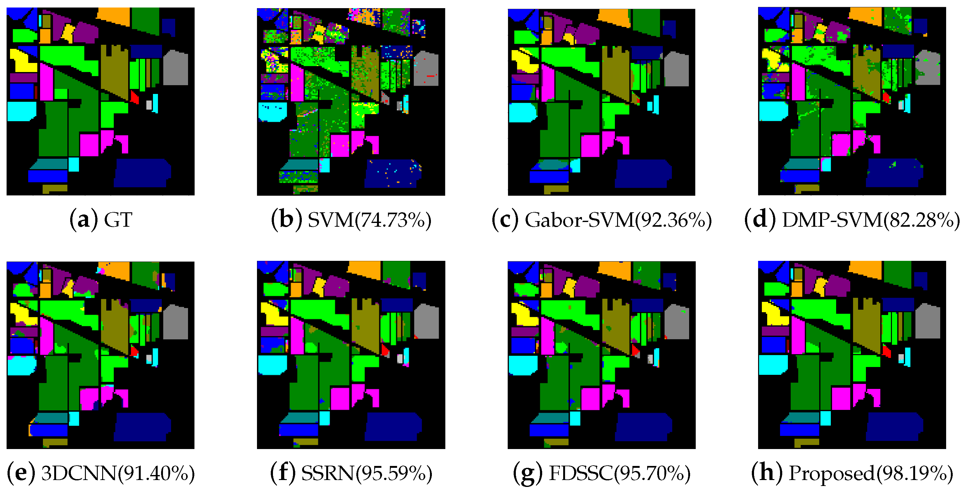
The results of IP dataset are reported in

Table 6. Class-specific results for the IP dataset using 5% training samples.

Class	Color	SVM	Gabor-SVM	DMP-SVM	3DCNN	SSRN	FDSSC	Proposed
1		27.78	100.0	0.00	93.94	86.49	87.88	100.0
2		66.78	91.29	70.89	87.32	96.35	97.72	97.10
3		72.45	86.86	88.35	95.45	96.60	93.32	99.03
4		45.10	90.09	100.0	95.72	97.18	94.93	92.20
5		82.94	93.66	98.94	88.76	99.26	99.51	99.26
6		84.11	98.29	92.21	93.21	97.44	98.93	98.20
7		100.0	0.00	0.00	100.0	88.89	100.0	81.25
8		87.63	98.15	98.53	99.54	97.48	95.70	100.0
9		72.73	0.00	0.00	90.0	100.0	100.0	85.71
10		73.64	91.82	91.08	88.72	93.20	92.84	98.00
11		68.35	90.21	68.12	94.61	94.93	96.55	98.46
12		66.29	85.08	89.63	76.39	84.95	82.86	98.15
13		88.04	100.0	100.0	95.05	100.0	100.0	100.0
14		92.50	97.83	96.81	94.83	99.56	99.21	99.74
15		66.16	98.19	96.47	83.51	94.04	95.04	96.12
16		98.61	88.24	100.0	100.0	100.0	98.82	97.67
OA		74.73	92.36	82.28	91.40	95.59	95.70	98.19
AA		74.57	81.86	74.44	92.32	95.39	95.83	96.31
kappa		0.7096	0.9124	0.7940	0.9019	0.9497	0.9510	0.9794

and the highest class-specific accuracies are in bold. Figure 7 shows the classification maps of different methods.

From Table 6, we can see that our method achieves the best performance, with 98.19% OA, 96.31% AA and 0.9794 Kappa. For SVM, it achieves the worst performance with only $74.73\%$ OA. Compared with the original SVM, the Gabor-SVM and DMP-SVM lead to a better performance because they also consider the spatial information for classification. However, the Gabor feature performs better than the DMP feature in terms of 3 indexes. For the four deep learning method, i.e., 3DCNN, SSRN, FDSSC and our method, 3DCNN is better than DMP-SVM with nearly $9\%$ improvement in OA but worse than Gabor-SVM. SSRN and FDSSC is better than 3DCNN with nearly $4\%$ improvement in OA. The reason of the FDSSC’s success in HSI classification can be concluded as the following: first, it extracts spectral feature and spatial feature separately. Second, the dense connection can deepen the structure. The two advantage ensures FDSSC can extract more discriminative features. However, our method, improves the OA $2.49\%$ compared with FDSSC and the other two indexs are also higher than FDSSC. Although our method achieves worse result than FDSSC in some classes, the OA, AA and kappa coefficient are the highest among these methods.

From the classification maps shown in Figure 7, ’salt-and-pepper’ noise is the worst for SVM due to the lack of incorporation of spatial information in the classification while the classification map of Gabor-SVM and DMP-SVM show more spatial continuity because they have consider the spatial information. Among these methods, our method shows least ’salt-and-pepper’ noise which corresponds to the result of Table 6.

4.3.2. Classification Maps and Result of UP Dataset

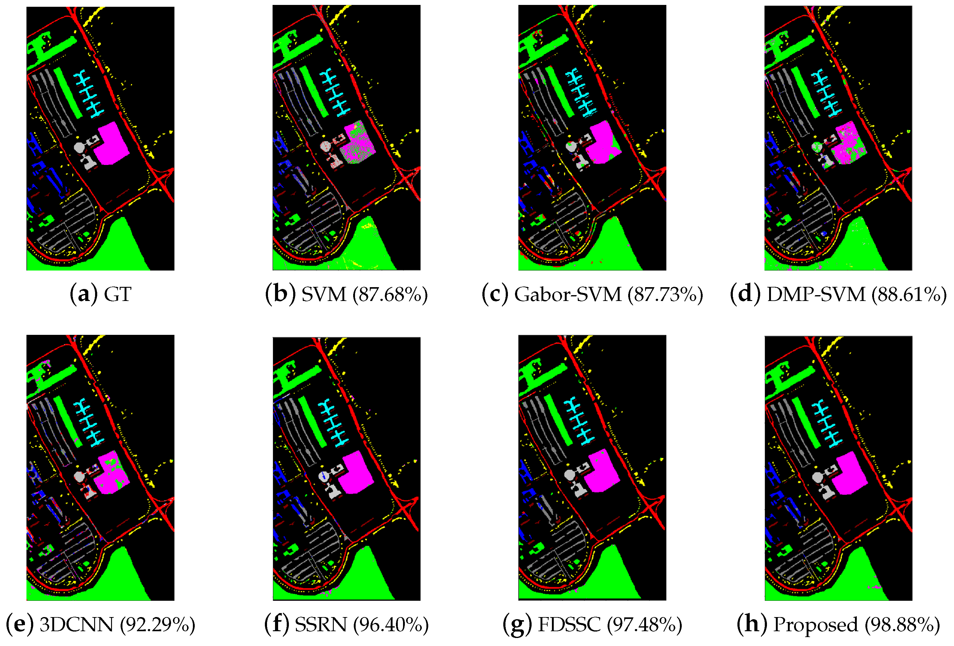
The results of the Pavia University dataset are reported in

Table 7. Class-specific results for the UP dataset using 1% training samples.

Class	Color	SVM	Gabor-SVM	DMP-SVM	3DCNN	SSRN	FDSSC	Proposed
1		93.72	77.61	89.74	88.17	99.67	99.48	99.37
2		93.36	92.93	89.95	97.08	98.61	98.79	99.73
3		65.61	87.13	81.20	75.29	79.16	99.64	99.16
4		87.48	77.60	97.45	97.88	100.0	100.0	98.21
5		98.89	88.11	99.92	100.0	100.0	99.92	100.0
6		83.71	96.12	85.19	93.97	95.83	98.66	97.45
7		62.96	89.27	67.73	75.35	92.57	94.36	100.0
8		74.55	83.94	81.76	79.88	88.20	84.67	95.12
9		100.0	56.41	96.20	97.27	99.57	100.0	99.36
OA		87.68	87.73	88.61	92.29	96.40	97.48	98.88
AA		84.48	83.24	87.68	89.43	94.85	97.28	98.71
kappa		0.8369	0.8363	0.8470	0.8974	0.9522	0.9666	0.9850

and the highest class-specific accuracies are in bold. The classification maps of different methods are shown in Figure 8.

From Table 7 we can see that our method achieves the best performance in terms of 3 index. For accuracy of every class, although our method has not achieved the best performance in every class, but for class 7, which have only 13 training samples, our method performs well, while other methods performed poor in this class. For class 8, other methods’ accuracy are all lower than $85\%$, which is a very low accuracy, but our method can achieve accuracy of 95%.

Although Gabor-SVM and DMP-SVM show little improvement in the aspect of OA, but the classification maps of them show more spatial continuity than SVM. For deep-learning-based models, 3DCNN improves OA about 4.5% compared with Gabor-SVM while FDSSC improves OA about 5% compared with 3DCNN which is very large improvement. However, our method achieves the highest performance in the three index among these methods.

4.3.3. Classification Maps and Results of SV Dataset

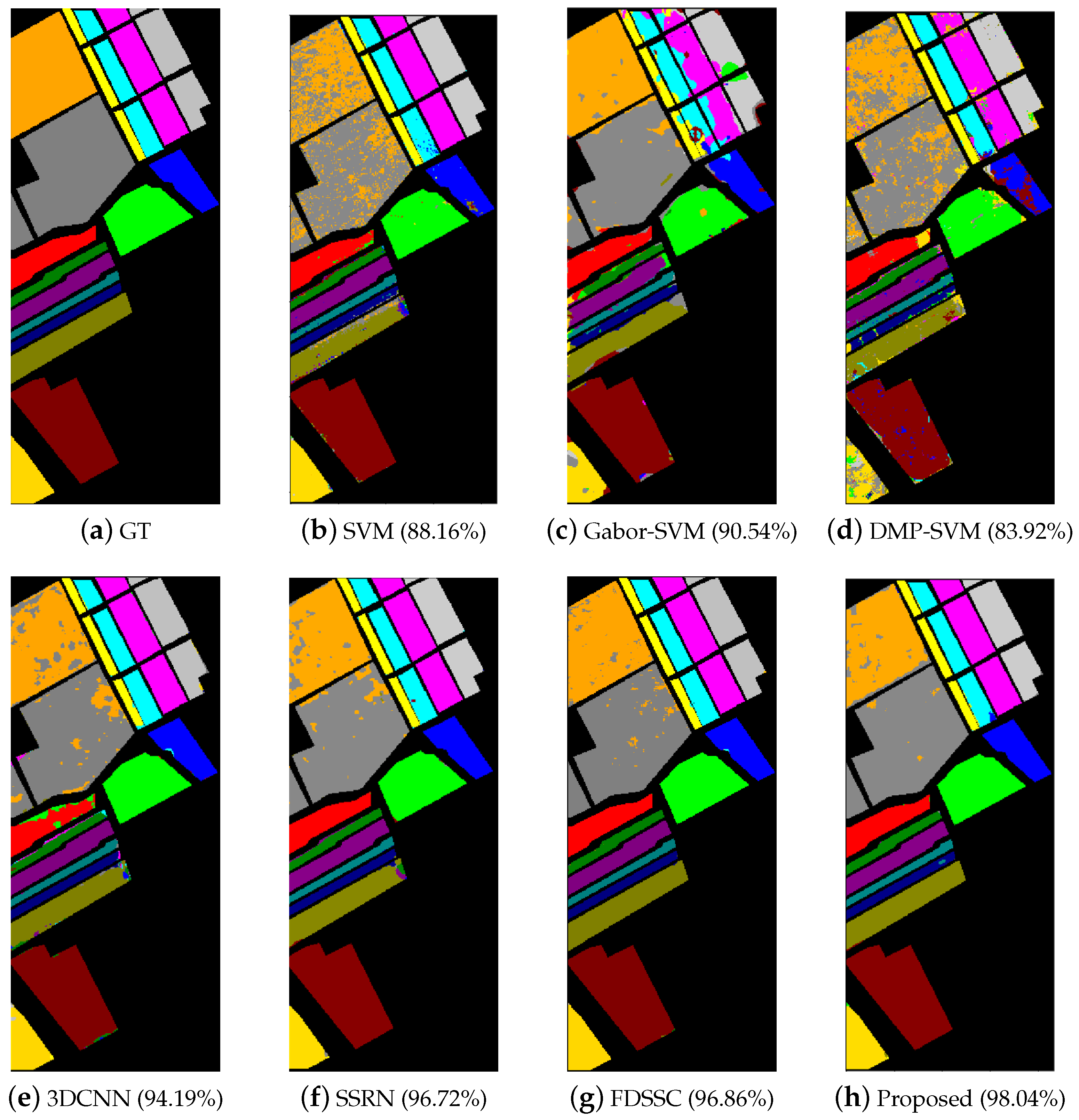
The results of the SV dataset are listed in

Table 8. Class-specific results for the SV dataset using 1% training samples.

Class	Color	SVM	Gabor-SVM	DMP-SVM	3DCNN	SSRN	FDSSC	Proposed
1		99.57	92.68	98.75	99.76	100.0	100.0	100.0
2		97.89	88.80	91.08	92.19	99.97	99.21	99.59
3		91.30	93.65	79.83	97.10	99.85	97.58	97.14
4		97.40	79.85	97.84	97.79	98.41	96.88	96.33
5		97.58	73.44	96.47	95.84	99.58	99.38	99.88
6		100.0	91.64	93.13	96.15	100.0	100.0	100.0
7		99.69	92.66	93.90	99.11	100.0	100.0	100.0
8		75.07	91.16	74.96	89.91	93.55	94.13	93.69
9		97.19	90.68	88.56	99.67	99.10	99.84	99.59
10		93.27	93.84	91.56	98.67	99.12	98.26	99.56
11		95.47	93.57	99.02	85.80	94.49	95.58	100.0
12		93.41	95.52	98.62	98.28	92.60	98.64	99.89
13		97.58	94.40	97.19	98.44	100.0	100.0	97.71
14		92.76	92.18	95.69	97.45	95.36	97.30	100.0
15		66.22	92.02	67.72	86.73	90.87	90.06	98.28
16		98.25	93.14	52.32	97.52	100.0	100.0	100.0
OA		88.16	90.54	83.92	94.19	96.72	96.86	98.04
AA		93.29	90.58	88.54	95.65	97.68	97.92	98.85
kappa		0.8680	0.8944	0.8204	0.9353	0.9635	0.9650	0.9782

and the highest class-specific accuracies are in bold. The classification maps of different methods are shown in Figure 9.

From Table 8 we can see that SVM, Gabor-SVM and DMP-SVM perform poorly in terms of OA, which are all below 91%. The classification maps of them also show large areas of mislabeled. This phenomenon has been avoided in 3DCNN, SSRN, FDSSC and our method. Furthermore, our method performs the best in terms of 3 indexes compared with other methods. In addition, the classification map of our method shows less mislabeled areas than other methods. For class 15, the accuracy of other method are all low than 93%, but our method can achieve the accuracy of 98.28%, which is the highest among these methods.

4.4. Investigation on Running Time

Table 9. Running time of SVM, Gabor-SVM, DMP-SVM, 3DCNN, SSRN, FDSSC, and our method on the IP dataset.

Dataset	Method	Training Times (s)	Test Times (s)
Indian Pines	SVM	5.9	1.20
	Gabor-SVM	5.0	0.74
	DMP-SVM	4.1	0.44
	3DCNN	381.0	25.96
	SSRN	361.4	8.15
	FDSSC	329.5	10.25
	proposed	314.2	10.85

,

Table 10. Running time of SVM, Gabor-SVM, DMP-SVM, 3DCNN, SSRN, FDSSC, and our method on the UP dataset.

Dataset	Method	Training Times (s)	Test Times (s)
Pavia University	SVM	4.2	2.06
	Gabor-SVM	4.8	2.50
	DMP-SVM	3.7	1.35
	3DCNN	375.6	33.48
	SSRN	352.5	26.54
	FDSSC	341.2	30.47
	proposed	317.4	31.82

and

Table 11. Running time of SVM, Gabor-SVM, DMP-SVM, 3DCNN, SSRN, FDSSC, and our method on the SV dataset.

Dataset	Method	Training Times(s)	Test Times(s)
Salinas	SVM	6.3	5.65
	Gabor-SVM	5.5	4.47
	DMP-SVM	4.3	2.43
	3DCNN	342.5	45.25
	SSRN	330.2	38.92
	FDSSC	325.8	41.13
	proposed	312.5	42.51

list the training and test time of the seven methods on the IP, UP and SV datasets, respectively. From Table 9, Table 10 and Table 11, we can find that SVM-based methods usually spend less time than deep-learning-based methods. Furthermore, Gabor-SVM and DMP-SVM spend less time than SVM because the length of Gabor-feature and DMP feature is shorter than the original feature. It has to be noted that, for Gabor-SVM and DMP-SVM, the training stage does not include the process of extracting the Gabor and DMP feature. For deep-learning-based methods, 3DCNN spends the most time due to the large input size and the large number of parameters to be trained. The training time and test time of SSRN and FDSSC is less than 3DCNN and the accuracy of them is much higher than 3DCNN, which proves the superiority of SSRN and FDSSC. FDSSC spends less time in training stage while more time in test stage compared with SSRN because the dense connected structure helps FDSSC to come to convergence more quickly, while FDSSC usually have more parameters which slows down the test speed. For our method, it spends less training time while gets much higher classification accuracy than FDSSC.

4.5. Investigation on the Number of Training

In Section 4.2, we have illustrated the effectiveness of our method, especially in the case of having a small number of training samples. In this part, we would further investigate the performance with different number of training samples.

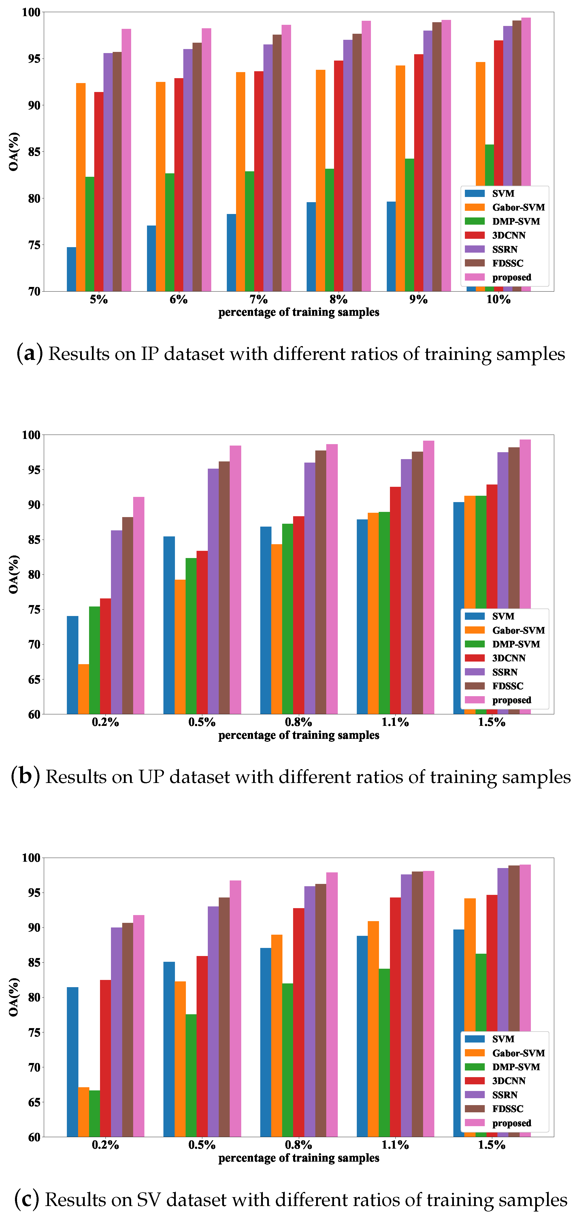
Figure 10 shows the experiment results. For IP dataset, the number of training samples per class is varied from 5% to 10% with an interval of 1%. For UP dataset and SV dataset, the number of training samples per class is varied from 0.2% to 1.4% with an interval of 0.3%.

As expected, with the training samples’ number increasing, the accuracy increases. We can see that no matter in what case, our method still performs better than other methods. From Figure 10a, we can see that SVM has the worst performance among the 7 methods and the OA is not higher than 80% in all cases. The Gabor-SVM outperforms DMP-SVM in all cases. With the number of training samples increasing, the 3DCNN gradually outperforms Gabor-SVM. The accuracy of FDSSC is slenderly higher than SSRN. Among these 7 methods, our method is always better than FDSSC in term of OA, especially in the circumstance of having very few training samples, which indicates the superiority of our method.

As is shown in Figure 10b, interestingly, Gabor-SVM performs worse than DMP-SVM and when the training samples are very few (i.e. 0.2%–0.5%), SVM performs better than DMP-SVM, Gabor-SVM and 3DCNN, which indicates that when the training samples is very few, the Gabor feature, DMP feature give little improvement for classification, 3DCNN is also not suitable in the case of having very few training samples, while SVM seems very suitable for classification in this case. In contrast with the aforementioned methods, FDSSC, SSRN and our method still perform well in all cases which indicates the stability of the 3 methods. Apparently, our method performs better than FDSSC and SSRN in all cases.

As is shown in Figure 10c, the same as UP dataset, SVM performs well in SV dataset, always better than DMP-SVM. For Gabor-SVM, when the training samples is very few, it performs worse than SVM, but with the training samples increasing, it outperforms SVM. Also, Gabor feature seems be more suitable for SV dataset than DMP feature. Among these methods, FDSSC, SSRN and our method still have good performance, which is much better than 3DCNN. Besides, our method achieves the highest accuracy in all cases.

Thus, our method is suitable in the circumstance when the number of training samples is limited.

4.6. Effectiveness of Channel Attention Mechanism and Spatial Attention Mechanism

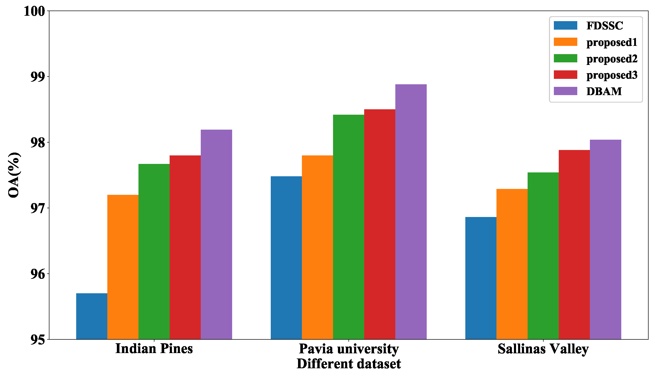
To validate the effectiveness of channel-wise attention mechanism and spatial-wise attention mechanism, we do three another experiments, i.e., without spectral attention and spatial attention (denoted as proposed1), only with spatial attention (denoted as proposed2) and only with spectral attention (denoted as proposed3). From Figure 11 we can see that without attention mechanism, the accuracy of three datasets will decrease in three dataset, which proves the effectiveness of attention mechanism. Furthermore, the spectral attention mechanism plays a more important role in HSI classification than spatial attention mechanism.

5. Conclusions

In this paper, a Double-Branch Multi-Attention mechanism network was proposed for HSI classification. It has two branches to extract spectral feature and spatial feature respectively, using densely connected 3D convolution layer with kernels of different sizes. Furthermore, according to the different purposes and characteristics of the two branches, the channel attention and spatial attention are applied in the two branches respectively to extract more discriminative feature. Our work is on the basic of FDSSC and CBAM. FDSSC is the state-of-the-art architecture in HSI classification, and CBAM is a novel and efficient attention network in image classification. Although it seems like a minor improvement, a lot of experiment results shows that our proposed method outperforms other state-of-the-art methods, especially in the case of having very few training samples. Furthermore, the training time is also reduced compared with the other two deep-learning methods because the attention blocks speed up the convergence of the network.

However, due to the attention block, the parameters of the network increase, which results in more time cost while testing stage. On the one hand, 3DCNN uses kernels of 3 dimensions and results in more parameters to train. To reduce the impact, we first reduce the spectral channels to 1 using 3D kernel with size of $1\times 1\times L$ (L represents the number of spectral channel), and set the kernel size of spectral domain to 1 in the dense spectral block. In our future work, we will try to use 2DCNN directly to extract spatial information. On the other hand, Recurrent Neural Network (RNN) seems more suitable for dealing with sequence data than CNN because it considers the order and relationship of the data. Obviously, HSI data can be regarded as sequence data and the relationship between different bands is useful for classification. In our future work, we will try to use RNN to extract spectral information.

References

- Wu, Y.; Ma, W.; Gong, M.; Su, L.; Jiao, L. A novel point-matching algorithm based on fast sample consensus for image registration. IEEE Geosci. Remote Sens. Lett. 2014, 12, 43–47. [Google Scholar] [CrossRef]
- Wu, Y.; Miao, Q.; Ma, W.; Gong, M.; Wang, S. PSOSAC: particle swarm optimization sample consensus algorithm for remote sensing image registration. IEEE Geosci. Remote Sens. Lett. 2017, 15, 242–246. [Google Scholar] [CrossRef]
- Ma, W.; Zhang, J.; Wu, Y.; Jiao, L.; Zhu, H.; Zhao, W. A Novel Two-Step Registration Method for Remote Sensing Images Based on Deep and Local Features. IEEE Trans. Geosc. Remote Sens. 2019. [Google Scholar] [CrossRef]
- Ma, W.; Xiong, Y.; Wu, Y.; Yang, H.; Zhang, X.; Jiao, L. Change Detection in Remote Sensing Images Based on Image Mapping and a Deep Capsule Network. Remote Sens. 2019, 11, 626. [Google Scholar] [CrossRef]
- Ma, W.; Yang, H.; Wu, Y.; Xiong, Y.; Hu, T.; Jiao, L.; Hou, B. Change Detection Based on Multi-Grained Cascade Forest and Multi-Scale Fusion for SAR Images. Remote Sens. 2019, 11, 142. [Google Scholar] [CrossRef]
- Ma, W.; Guo, Q.; Wu, Y.; Zhao, W.; Zhang, X.; Jiao, L. A Novel Multi-Model Decision Fusion Network for Object Detection in Remote Sensing Images. Remote Sens. 2019, 11, 737. [Google Scholar] [CrossRef]
- Li, Z.; Huang, L.; He, J. A Multiscale Deep Middle-level Feature Fusion Network for Hyperspectral Classification. Remote Sens. 2019, 11, 695. [Google Scholar] [CrossRef]
- Awad, M.; Jomaa, I.; Arab, F. Improved Capability in Stone Pine Forest Mapping and Management in Lebanon Using Hyperspectral CHRIS-Proba Data Relative to Landsat ETM+. Photogramm. Eng. Remote Sens. 2014, 80, 725–731. [Google Scholar] [CrossRef]
- Liang, H.; Li, Q. Hyperspectral imagery classification using sparse representations of convolutional neural network features. Remote Sens. 2016, 8, 99. [Google Scholar] [CrossRef]
- Sun, W.; Yang, G.; Du, B.; Zhang, L.; Zhang, L. A sparse and low-rank near-isometric linear embedding method for feature extraction in hyperspectral imagery classification. IEEE Trans. Geosc. Remote Sens. 2017, 55, 4032–4046. [Google Scholar] [CrossRef]
- Marinelli, D.; Bovolo, F.; Bruzzone, L. A Novel Change Detection Method for Multitemporal Hyperspectral Images Based on Binary Hyperspectral Change Vectors. IEEE Trans. Geosc. Remote Sens. 2019. [Google Scholar] [CrossRef]
- Zhao, C.; Wang, Y.; Qi, B.; Wang, J. Global and local real-time anomaly detectors for hyperspectral remote sensing imagery. Remote Sens. 2015, 7, 3966–3985. [Google Scholar] [CrossRef]
- Awad, M. Sea water chlorophyll-a estimation using hyperspectral images and supervised artificial neural network. Ecol. Inform. 2014, 24, 60–68. [Google Scholar] [CrossRef]
- Li, W.; Du, Q. Gabor-filtering-based nearest regularized subspace for hyperspectral image classification. IEEE J. Sel. Top. Appl. Earth Obs. Remote Sens. 2014, 7, 1012–1022. [Google Scholar] [CrossRef]
- Benediktsson, J.A.; Pesaresi, M.; Amason, K. Classification and feature extraction for remote sensing images from urban areas based on morphological transformations. IEEE Trans. Geoscie. Remote Sens. 2003, 41, 1940–1949. [Google Scholar] [CrossRef] [Green Version]
- Sidike, P.; Chen, C.; Asari, V.; Xu, Y.; Li, W. Classification of hyperspectral image using multiscale spatial texture features. In Proceedings of the 2016 8th Workshop on Hyperspectral Image and Signal Processing: Evolution in Remote Sensing (WHISPERS), Los Angeles, CA, USA, 21–24 August 2016; pp. 1–4. [Google Scholar]
- Chen, Y.; Lin, Z.; Zhao, X.; Wang, G.; Gu, Y. Deep learning-based classification of hyperspectral data. IEEE J. Sel. Top. Appl. Earth Obs. Remote Sens. 2014, 7, 2094–2107. [Google Scholar] [CrossRef]
- Chen, Y.; Zhao, X.; Jia, X. Spectral–spatial classification of hyperspectral data based on deep belief network. IEEE J. Sel. Top. Appl. Earth Obs. Remote Sens. 2015, 8, 2381–2392. [Google Scholar] [CrossRef]
- Tao, C.; Pan, H.; Li, Y.; Zou, Z. Unsupervised spectral–spatial feature learning with stacked sparse autoencoder for hyperspectral imagery classification. IEEE Geosci. Remote Sens. Lett. 2015, 12, 2438–2442. [Google Scholar]
- Ma, X.; Wang, H.; Geng, J. Spectral–spatial classification of hyperspectral image based on deep auto-encoder. IEEE J. Sel. Top. Appl. Earth Obs. Remote Sens. 2016, 9, 4073–4085. [Google Scholar] [CrossRef]
- Zhang, X.; Liang, Y.; Li, C.; Huyan, N.; Jiao, L.; Zhou, H. Recursive Autoencoders-Based Unsupervised Feature Learning for Hyperspectral Image Classification. IEEE Geosci. Remote Sens. Lett. 2017, 14, 1928–1932. [Google Scholar] [CrossRef] [Green Version]
- Sidike, P.; Asari, V.K.; Sagan, V. Progressively Expanded Neural Network (PEN Net) for hyperspectral image classification: A new neural network paradigm for remote sensing image analysis. ISPRS J. Photogramm. Remote Sens. 2018, 146, 161–181. [Google Scholar] [CrossRef]
- Hu, W.; Huang, Y.; Wei, L.; Zhang, F.; Li, H. Deep convolutional neural networks for hyperspectral image classification. J. Sens. 2015, 2015. [Google Scholar] [CrossRef]
- Chen, Y.; Jiang, H.; Li, C.; Jia, X.; Ghamisi, P. Deep feature extraction and classification of hyperspectral images based on convolutional neural networks. IEEE Trans. Geosci. Remote Sens. 2016, 54, 6232–6251. [Google Scholar] [CrossRef]
- Paoletti, M.E.; Haut, J.M.; Fernandez-Beltran, R.; Plaza, J.; Plaza, A.J.; Pla, F. Deep pyramidal residual networks for spectral-spatial hyperspectral image classification. IEEE Trans. Geosci. Remote Sens. 2019, 57, 740–754. [Google Scholar] [CrossRef]
- Haut, J.M.; Paoletti, M.E.; Plaza, J.; Li, J.; Plaza, A. Active learning with convolutional neural networks for hyperspectral image classification using a new bayesian approach. IEEE Trans. Geosci. Remote Sens. 2018, 56, 6440–6441. [Google Scholar] [CrossRef]
- Yang, S.; Feng, Z.; Wang, M.; Zhang, K. Self-paced learning-based probability subspace projection for hyperspectral image classification. IEEE Trans. Neural Netw. Learn. Syst. 2019, 30, 630–635. [Google Scholar] [CrossRef]
- Tan, K.; Hu, J.; Li, J.; Du, P. A novel semi-supervised hyperspectral image classification approach based on spatial neighborhood information and classifier combination. ISPRS J. Photogramm. Remote Sens. 2015, 105, 19–29. [Google Scholar] [CrossRef]
- Zhang, M.; Gong, M.; Mao, Y.; Li, J.; Wu, Y. Unsupervised Feature Extraction in Hyperspectral Images Based on Wasserstein Generative Adversarial Network. IEEE Trans. Geosci. Remote Sens. 2018. [Google Scholar] [CrossRef]
- Shi, C.; Pun, C.M. Superpixel-based 3D deep neural networks for hyperspectral image classification. Pattern Recognit. 2018, 74, 600–616. [Google Scholar] [CrossRef]
- Jiang, J.; Ma, J.; Chen, C.; Wang, Z.; Cai, Z.; Wang, L. SuperPCA: A superpixelwise PCA approach for unsupervised feature extraction of hyperspectral imagery. IEEE Trans. Geosci. Remote Sens. 2018, 56, 4581–4593. [Google Scholar] [CrossRef]
- Jiang, J.; Ma, J.; Wang, Z.; Chen, C.; Liu, X. Hyperspectral image classification in the presence of noisy labels. IEEE Trans. Geosci. Remote Sens. 2019, 57, 851–865. [Google Scholar] [CrossRef]
- He, K.; Zhang, X.; Ren, S.; Sun, J. Deep residual learning for image recognition. In Proceedings of the IEEE Conference on Computer Vision and Pattern Recognition, Las Vegas, NV, USA, 26 June–1 July 2016; pp. 770–778. [Google Scholar]
- Zhong, Z.; Li, J.; Luo, Z.; Chapman, M. Spectral–Spatial Residual Network for Hyperspectral Image Classification: A 3-D Deep Learning Framework. IEEE Trans. Geosci. Remote Sens. 2018, 56, 847–858. [Google Scholar] [CrossRef]
- Huang, G.; Liu, Z.; Van Der Maaten, L.; Weinberger, K.Q. Densely connected convolutional networks. In Proceedings of the IEEE Conference on Computer Vision and Pattern Recognition, Honolulu, HI, USA, 21–26 July 2017; pp. 4700–4708. [Google Scholar]
- Wang, W.; Dou, S.; Jiang, Z.; Sun, L. A Fast Dense Spectral–Spatial Convolution Network Framework for Hyperspectral Images Classification. Remote Sens. 2018, 10, 1068. [Google Scholar] [CrossRef]
- Fang, B.; Li, Y.; Zhang, H.; Chan, J.C.W. Hyperspectral Images Classification Based on Dense Convolutional Networks with Spectral-Wise Attention Mechanism. Remote Sens. 2019, 11, 159. [Google Scholar] [CrossRef]
- Woo, S.; Park, J.; Lee, J.Y.; So Kweon, I. Cbam: Convolutional block attention module. In Proceedings of the European Conference on Computer Vision (ECCV), Munich, Germany, 8–14 September 2018; pp. 3–19. [Google Scholar]
- Mnih, V.; Heess, N.; Graves, A. Recurrent models of visual attention. Adv. Neural Inf. Process. Syst. 2014, 2204–2212. [Google Scholar]
- Xu, K.; Ba, J.; Kiros, R.; Cho, K.; Courville, A.; Salakhudinov, R.; Zemel, R.; Bengio, Y. Show, attend and tell: Neural image caption generation with visual attention. In Proceedings of the International Conference on Machine Learning, Lille, France, 6–11 July 2015; pp. 2048–2057. [Google Scholar]
- Zhu, Y.; Groth, O.; Bernstein, M.; Fei-Fei, L. Visual7w: Grounded question answering in images. In Proceedings of the IEEE Conference on Computer Vision and Pattern Recognition, Las Vegas, NV, USA, 26 June–1 July 2016; pp. 4995–5004. [Google Scholar]
- Yang, Z.; He, X.; Gao, J.; Deng, L.; Smola, A. Stacked attention networks for image question answering. In Proceedings of the IEEE Conference on Computer Vision and Pattern Recognition, Las Vegas, NV, USA, 26 June–1 July 2016; pp. 21–29. [Google Scholar]
- Nam, H.; Ha, J.W.; Kim, J. Dual attention networks for multimodal reasoning and matching. In Proceedings of the IEEE Conference on Computer Vision and Pattern Recognition, Honolulu, HI, USA, 21–26 July 2017; pp. 299–307. [Google Scholar]
- Melgani, F.; Bruzzone, L. Classification of hyperspectral remote sensing images with support vector machines. IEEE Trans. Geosci. Remote Sens. 2004, 42, 1778–1790. [Google Scholar] [CrossRef] [Green Version]
- Bau, T.C.; Sarkar, S.; Healey, G. Hyperspectral region classification using a three-dimensional Gabor filterbank. IEEE Trans. Geosci. Remote Sens. 2010, 48, 3457–3464. [Google Scholar] [CrossRef]
- Fauvel, M.; Benediktsson, J.A.; Chanussot, J.; Sveinsson, J.R. Spectral and spatial classification of hyperspectral data using SVMs and morphological profiles. IEEE Trans. Geosci. Remote Sens. 2008, 46, 3804–3814. [Google Scholar] [CrossRef]
Figure 1.
Comparison of Residual connection and Dense connection.
Figure 2.
Structure of the Fast Dense Spectral–Spatial Convolution Network.
Figure 3.
Structure of channel-wise attention.
Figure 4.
Structure of spatial-wise attention.
Figure 5.
The training procedure of our method.
Figure 6.
Structure of DBMA network. The top branch is called Spectral Branch consisting of dense spectral block and channel attention block, which is used to extract spectral feature. The bottom branch is called Spatial Branch consisting of dense spatial block and spatial attention block, which is used to extract spatial feature.
Figure 7.
Classification maps of the IP dataset with 5% training samples. The first image (a) represents ground-truth (GT) and images from (b)–(h) are the classification maps using different methods.
Figure 8.
Classification maps of the UP dataset using 1% training samples. The first image (a) represents ground-truth (GT) and images from (b)–(h) are the classification maps using different methods.
Figure 9.
Classification maps of The SV dataset. The first image (a) represents ground-truth (GT) and images from (b)–(h) are the classification maps using different methods.
Figure 10.
TheOA results of SVM, Gabor-SVM, DMP-SVM, 3DCNN, SSRN, FDSSC and proposedmethod with different number of training samples on the (a) IP dataset, (b) UP dataset, and (c) SV dataset.
Figure 11.
Effect of different attention mechanism on different datasets.