Multi-Spectral Lidar: Radiometric Calibration, Canopy Spectral Reflectance, and Vegetation Vertical SVI Profiles


1
Department of Geography, University of Lethbridge, Lethbridge, AB T1K 3M4, Canada
2
Institute of Mathematical Problems of Biology RAS, branch of the M.V.Keldysh Institute of Applied Mathematics of the Russian Academy of Sciences, 1 Prof. Vitkevich St, Pushchino, Moscow Region 142290, Russia
*
Author to whom correspondence should be addressed.
Remote Sens. 2019, 11(13), 1556; https://doi.org/10.3390/rs11131556
Submission received: 31 May 2019
/
Revised: 27 June 2019
/
Accepted: 28 June 2019
/
Published: 30 June 2019
(This article belongs to the Special Issue Future Trends and Applications for Airborne Laser Scanning)
Abstract
:Multi-spectral (ms) airborne lidar data are enriched relative to traditional lidar due to the multiple channels of intensity digital numbers (DNs), which offer the potential for active Spectral Vegetation Indices (SVIs), enhanced classification, and change monitoring. However, in case of SVIs, indices should be calculated from spectral reflectance values derived from intensity DNs after calibration. In this paper, radiometric calibration of multi-spectral airborne lidar data is presented. A novel low-cost diffuse reflectance coating was adopted for creating radiometric targets. Comparability of spectral reflectance values derived from ms lidar data for coniferous stand (2.5% for 532 nm, 17.6% for 1064 nm, and 8.4% for 1550 nm) to available spectral libraries is shown. Active vertical profiles of SVIs were constructed and compared to modeled results available in the literature. The potential for a new landscape-level active 3D SVI voxel approach is demonstrated. Results of a field experiment with complex radiometric targets for estimating losses in detected lidar signals are described. Finally, an approach for estimating spectral reflectance values from lidar split returns is analyzed and the results show similarity of estimated values of spectral reflectance derived from split returns to spectral reflectance values obtained from single returns (p > 0.05 for paired test).
1. Introduction
Light Detection and Ranging (lidar) established itself as a unique high-resolution remote sensing technology due to its 3D sampling of terrain and its ability to characterize overlying vegetation structure from treetop to ground [1]. Lidar is primarily used to construct detailed digital elevation models (DEMs), but the intensity channel (an index of signal reflectance) is increasingly used in a similar fashion to black and white aerial photographs or single bands in multispectral imagery. In passive imagery, numerous Spectral Vegetation Indices (SVIs) have been developed based on reflectance values derived from image-based digital numbers (DNs) as quantitative indicators of vegetation phenology, including long-term patterns of loss or growth of photosynthesizing foliage [2]. Modern multi-spectral (ms) lidar technology allows for active vertical spectral sampling of vegetation profiles opening new application prospects in forest inventory, habitat mapping, tree species classification, forest health assessment, and biomass and carbon stock estimation [3,4,5]. However, it is well known that when the data are collected with different sensors or sensor parameters, at different locations or at different times, the consistency of the obtained spectral information and its derivatives is not assured [6,7,8]. Meanwhile, for developing comparable models [9], classification and change detection [10], and monitoring of yield curves and vegetation health [7,11,12], it is necessary to normalize spectral information (intensity) from each channel or sensor [4,13].
In recent years, a few publications have considered multi-spectral lidar for land surface classification using traditional optical classification approaches [4,14,15], as well as the development of active SVIs [16,17]. Within a forestry context, active SVIs, specifically active normalized difference vegetation indices (NDVIs), have been successfully used for classification of vegetation [18]. Moreover, a potential of measuring plant physiology, leaf moisture content, and leaf-bark separation by generating vertical profiles of spectral indices was shown through modeling and lab experiments [19,20,21]. This potential exists because spectral vegetation indices can be linked to plant pigment concentration and leaf moisture content. However, for consistency over time and comparability with other sensors and data sets, SVIs should be calculated with spectral reflectance derived from the lidar intensity DNs after rigorous radiometric correction [22]. For traditional single-channel lidar (e.g., 1064 nm wavelength systems), there is over a decade of published research into target-based radiometric calibration [23,24,25], but such approaches have yet to be applied in operational ms lidar SVI derivation.
Currently, two types of data output are available: Discrete-return (DR) sensor-supplied intensity values as an index of the peak signal amplitude, (i.e., not the time-integrated backscattered light response); and full waveform (FWF) intensity profile samples (typically 1 ns interval) of the detected intensity signal. However, even FWF data with additional return pulse width information cannot directly resolve the ambiguity in intensity response between area of contact of the split return and target spectral reflectance. This constrains the analysis and interpretation of split return intensities for SVI derivation, as it is impossible to know a priori if the intensity of any individual return is mostly a function of contact area or spectral reflectance. However, if the spectral reflectance value of one out of two split returns is a priori known, then, assuming homogeneous footprint illumination, it is theoretically possible to reconstruct both illuminated areas and calculate the unknown target spectral reflectance using the following equations:
Here ρ1 is the spectral reflectance of the first point target, ρ0 is the spectral reflectance of the known target, A0 is the illuminated area of the whole footprint at nadir, A2 is the illuminated area of the second target at nadir; I0, I1, and I2 are, respectively, the intensity responses of the single return from the extended target, intensity of the first return, and the intensity of the last return from the target with the same spectral reflectance as ρ0. For volumetric returns, the above equations should include pulse width, substituting intensity values with calculated energy from a particular target cluster. A similar approach was utilized by [26] to introduce a new method of calculating total canopy transmittance based only on the energy of ground returns. However, Equation (1) has never been rigorously tested in an experiment with a target of known reflectance. If such a simple algorithm proves valid, it opens up the potential to derive spectral reflectance values for split returns with some a priori assumptions and, consequently, increases the number of returns available for SVI calculation or robust classification from a particular survey.
To explore issues associated with comparability of lidar derived reflectance, ms lidar data were collected using a Teledyne Optech Titan sensor over an area of interest (AOI) with installed radiometric targets on 7 August 2016. This experiment addressed the following research objectives: (i) To develop large scale radiometric calibration targets and test them during an ms lidar data acquisition campaign; (ii) to derive spectral reflectance (or spectral pseudo-reflectance) values from calibrated ms lidar intensity DNs and compare them to ground spectral reflectance obtained by passive hyperspectral sensors available in public spectral libraries; (iii) to develop plot level active vertical SVI profiles of vegetation from actual field data and compare them to modeled [20] and lab [21] results published in the literature; (iv) to develop voxel data structure of active 3D SVIs and demonstrate its potential on landscape level; and (v) to set up an experiment with complex radiometric targets for assessing feasibility of estimating spectral reflectance from split returns based on Equation (1) and explore energy losses of lidar backscatter signal in the canopy.
2. Data and Methods
2.1. Radiometric Calibration Targets
Although there are plenty of options for lidar radiometric calibration targets described in the literature [23,27], a new version was adopted based on a low-cost diffuse reflective coating developed by [28]. This technique is similar to work by [29] and could be considered a low-cost operational alternative to Spectralon® targets. In comparison to passive airborne remote sensing, airborne lidar requires larger radiometric targets due to the relatively large footprint size (Table 1), and the associated cost can become prohibitive in some cases. Lidar allows volumetric sampling (e.g., in the case of vegetation) and investigation of radiometric response requires targets of custom shape, dimension and elevation. A diffuse reflective coating allows flexibility in constructing such custom radiometric targets. In this project, it was not possible to follow the coating recipe precisely because some of the products are no longer available. Anatase TiO2 pigment (Kronos® 1000, Kronos Worldwide Inc., Dallas, TX, USA) and a water-borne polyurethane binder (Varathane® Interior Diamond Finish Water-based polyurethane) were used. Water based white latex primer (Glidden Vantage®, PPG Industries Inc., Pittsburgh, PA, USA) was used as the base layer and three layers of coating were put on top using a roller. The spectral reflectance of the targets was validated in the lab using an Analytical Spectral Devices (ASD) FieldSpec full-range spectroradiometer (ASD Inc., Boulder, CO, USA) by comparison with a “white” Spectralon® (Labspere Inc., North Sutton, NH, USA) panel of known spectral reflectance values (~99%).
2.2. Radiometric Calibration Target Experimental Configuration
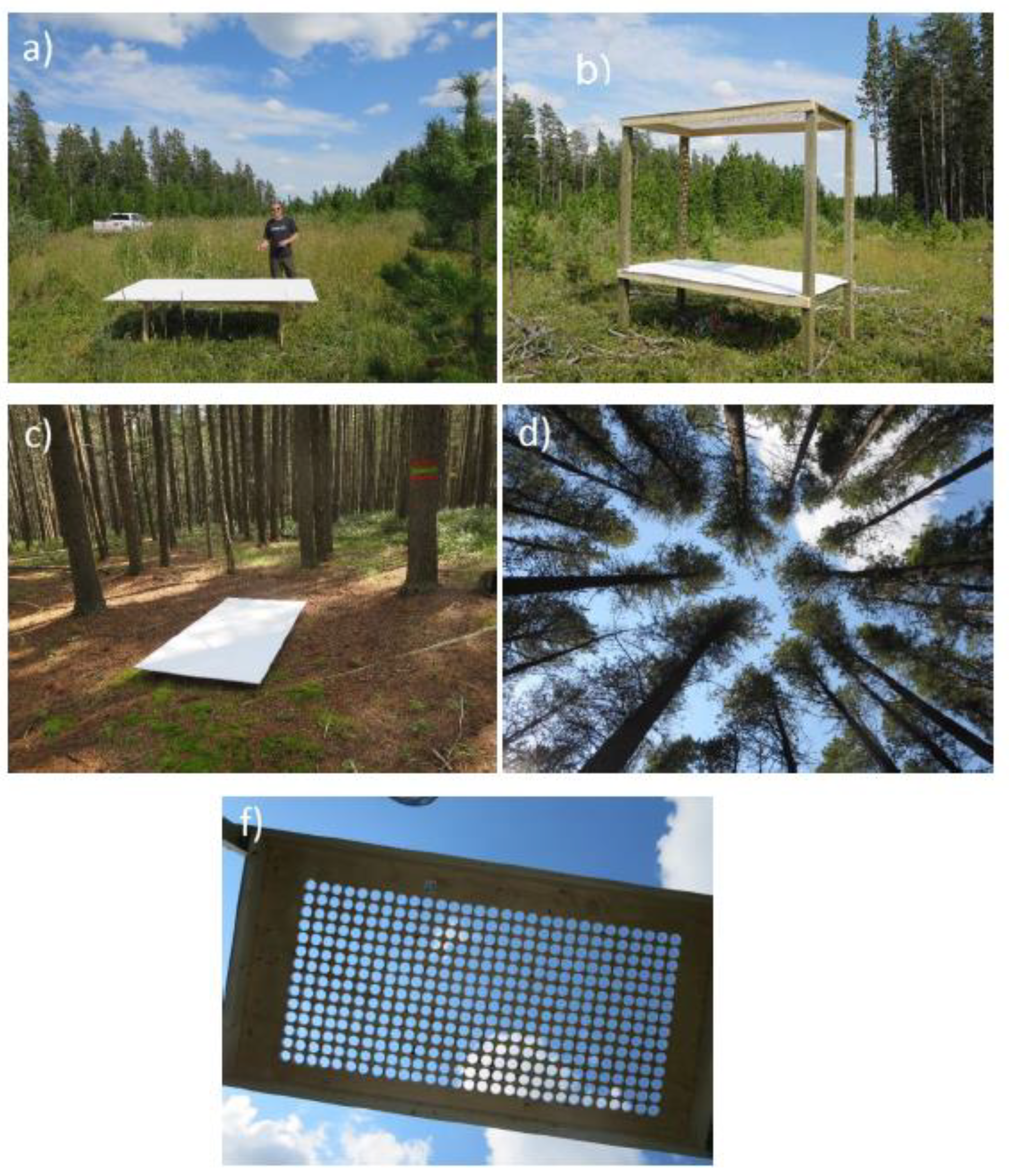
Radiometric non-transparent targets were constructed from 8′ by 4′ plywood sheets and covered with a diffuse white coating as described above. To analyze split-return characteristics of pulses passing through foliage, an additional elevated partial reflector surface target was constructed with an accurately known 50% transmittance, achieved by drilling 2.5” holes in the plywood sheet. Drilled 50% transmittance target was mounted 2 m above non-transparent target (Figure 1b,f). One non-transparent radiometric target was installed beneath the forest canopy, while another non-transparent target together with the elevated 50% transmittance target was installed in a nearby clearing (Figure 1).
2.3. Study Area and Lidar Data Collection
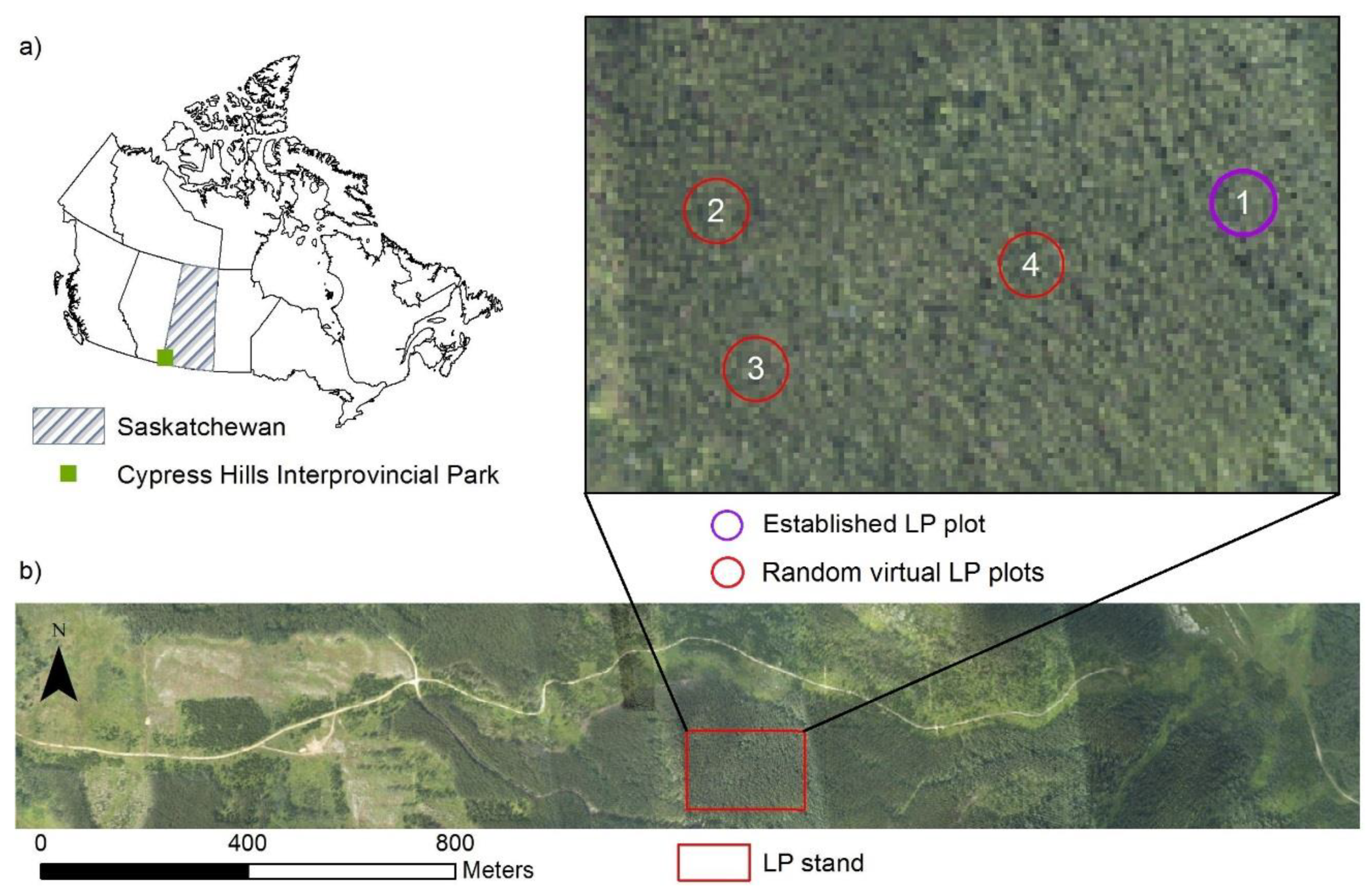
The study was conducted in Cypress Hills Interprovincial Park (SK, Canada), 75 km north of the US border (Figure 2a). The Cypress Hills is a unique geological formation which rises on average 600 m above the surrounding plains [30]. There are four species of trees in the Cypress Hills, two of which are coniferous. The lodgepole pine (Pinus contorta), which is typically found in the Rocky Mountains. The second coniferous species is white spruce (Picea glauca). There are two main deciduous tree species in the Cypress Hills, trembling aspen (Populus tremuloides) and balsam poplar (Populus balsamifera). Almost 70% of the AOI (Figure 2b) is covered with mature lodgepole pine (LP) forest. A stand of uniform LP cover was selected for further analysis (Figure 2b). One circle plot of 11.3 m radii (a standard size and shape for a mensuration plot in forest inventory) was established inside the stand with 58 LP trees of average stem height 20.9 m and average DBH (Diameter at Breast Height) of 21 cm. The plot displayed no developed understory and a uniform upper canopy (Figure 1c,d); the ground surface was flat. Three additional virtual plots were chosen in random locations within the LP stand for further comparison (Figure 2b).
Discrete return multi-spectral lidar data were collected at three wavelengths (532 nm, 1064 nm, and 1550 nm) using a Teledyne Optech Titan system on 7 August 2016 at an average flying altitude of 600 m AGL. Relevant sensor characteristics are presented in Table 1, and a detailed description of the Titan can be found in [31]. Data were collected at 100 kHz per channel with a variable scan angle (from ±22 to ±27 degree) and scan frequency (from 29 to 35 Hz). Flight lines were spaced to achieve approximately 50% side-lap (i.e., 200% coverage). Average aircraft speed varied from 63 to 72 m/s depending on the flight line direction due to strong winds. Following [32], return sampling point density over vegetation is compared to pulse emission density as a description of the dataset and average values are presented in Table 2.
Raw data in the form of a range file and Smoothed Best Estimate Trajectory file (SBET) were processed in Lidar Mapping Suite (LMS, proprietary software from Teledyne Optech) and after block adjustment, point cloud data were obtained with verified accuracy (over available rooftops) of RMSE <0.06 m in horizontal separation and RMSE <0.04 m in height separation.
2.4. Analysis
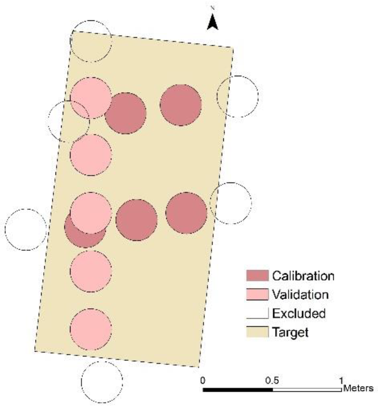
Lidar data were output from LMS in LAS format with intensities normalized to a range of 600 m. Firstly, due to a scan line intensity banding effect [32,33], half of the points were marked as compromised and omitted from the analysis. Locations of the targets were surveyed with a dual frequency Topcon Hiper SR survey-grade Global Navigation Satellite System (GNSS) receiver and coordinates of the target corners were post-processed using Precise Point Positioning (PPP [34], sigma values <0.2 m). Returns from the targets were manually selected based on their spatial coincidence and proximity to the target border. Those that illuminated edges of the targets were excluded. Only points with the entire footprint (1/e2, Gaussian shape; Table 1) on a given target were used in the analysis (Figure 3). Three flight lines provided returns from the targets; two because of the planned 50% overlap between lines and an additional crossline, which was planned for increasing the number of calibration target hits.
As a first step, DN values corresponding to 100% spectral reflectance were derived for open target hits from two lines, leaving the cross line open target hits for verification. The DN value () corresponding to 100% spectral reflectance and normalized to the inverse square range (ℝ) can be written in the form:
with index l running through the three ms lidar channels and index k through selected points over the calibration target; I denotes intensity DN, angle ϑ the angle between the source and the target, and the known value of the calibrated target spectral reflectance for each channel. Consequently, all single-return intensity DNs from every point (index k) can be normalized with respect to the above value by the following formula:
Here, represents a spectral pseudo-reflectance of a target at a particular wavelength/channel (index l); i.e., a peak of the backscatter signal, normalized to the response of an ideal diffuse Lambertian target of 100% reflectance and normal to the lidar beam propagation direction.
Spectral pseudo-reflectance of LP stands (Figure 2) was calculated from single returns separately for all points from treetop to ground, and then only for the canopy (returns higher than 10 m above ground). The resulting two point clouds were gridded into 15 m pixel spectral reflectance raster maps (overall 150 pixels) with average values of spectral pseudo-reflectance assigned to each pixel. Then, the mean values of spectral pseudo-reflectance for both maps were compared to Airborne Visible/InfraRed Imaging Spectrometer (AVIRIS), AISA Dual (Specim, Spectral Imaging Ltd.), and ASD field portable spectrometer (ASD Inc., Boulder, Colorado) data. AVIRIS with 15 m resolution [35] for mature LP stands (45–150 years old, noted as LP1 in [35]) from Yellowstone National Park (YNP) and ASD data for a stack of live LP needles [36] were retrieved from United States Geological Survey (USGS) spectral library. AISA Dual hyperspectral sensor data with 2 m resolution for pines (unspecified species) from the North Thompson, BC were received from Professor Olaf Niemann (Hyperspectral-LiDAR Research Group, University of Victoria; personal communication). In addition, histograms of spectral pseudo-reflectance for all single returns from the canopy inside an LP plot (only returns which were higher than 10 m above ground) were output.
For developing vertical normalized differences, the vertical distribution of each channel for the established LP plot was analyzed, and after finding a lower canopy threshold, the returns were binned in 0.5 m increments (index h). Then, from the average of each bin spectral pseudo-reflectance value , normalized differences were calculated using the following formula (indices l and m run through Titans channels; see [32] for detailed explanation of ):
The same procedure was repeated for three additional randomly selected virtual LP plots (Figure 2b).
For the lifted target, after normalization of each return toward the cosine of the incident angle, the sum of the pseudo-intensity values of split returns were compared with the known spectral reflectance of the open target. For the below-canopy target, single returns were compared with the returns from the open target, and double and triple returns (with an assumption for triple returns that first and second returns detected the same surface type) were used for deriving spectral reflectance values of the canopy using Equation (1). To illustrate the ms lidar canopy voxelization approach, two types of map were created at 20 m resolution: Ground nδ(C2,C1) map; and (canopy nδ(C2,C1) and nδ(C2,C3) maps (see [32] for the conventions used). For the ground map, only single returns from ground returns and those up to 0.5 m above the ground level were used. Ground nδ(C2,C1) map was visually compared with the Digital Terrain Model (DTM) at 2 m resolution, and with low resolution Topographic Positioning Index (TPI) derived from the 20 m resolution DTM. For canopy maps, single returns penetrated up to almost the full depth profile of the canopy, with few single returns 2 m above the ground. A two-sample Kolmogorov-Smirnov test on point height distributions for each pair of all three channels was performed to find the practical threshold value for canopy height range where vertical intensity distributions from different channels can be compared. In addition, a vertical profile of nδ(C2,C1) was constructed with Equation (5) along a 20 m wide transect, with voxels of 20 by 20 m in plane and 0.5 m in height.
3. Results and Discussion
3.1. Radiometric Calibration Targets
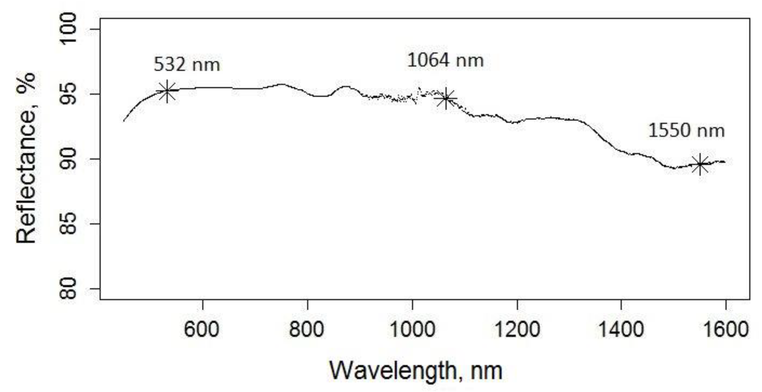
A spectral reflectance curve of the target obtained from laboratory measurements is presented in Figure 4. Values of spectral reflectance with RMSE of measurements for Titan’s wavelengths are presented in Table 3. Spectral reflectance values of the constructed target are similar to those reported by [28].
3.2. Verification of the Intensity Normalization
Calculated values of for each channel together with the cosine corrected spectral reflectance validation derived for the open target hits from the crossline are presented in Table 4. These values are comparable with the spectral reflectance measured in the laboratory using an ASD (Table 3).
The derived spectral reflectance values differ by 0.5% for C1, 1.4% for C2, and 2.1 % for C3 (Table 3 and Table 4). The derived target spectral reflectance was higher than lab-measured for the C1 and C2 channels and lower for the C3 channel. Since one of the lines used to derive the calibration value was flown 80 m lower than the second line and the crossline used for the verification, one would expect that all derived values should be lower. Accounting for the difference in atmospheric losses may improve the results. However, it is assumed here that the 0.5–2.1% differences between lab- and field-calibrated target spectral reflectance is sufficient for constructing SVIs.
3.3. Spectral Pseudo-Reflectance Derived from Titan Compared to Hyperspectral Sensor Data
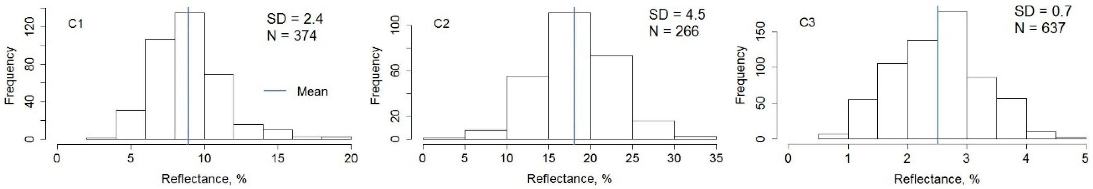
Comparison of Titan’s derived spectral pseudo-reflectance to the AVIRIS, AISA dual, and ASD data is shown in Table 5. Histograms of spectral pseudo-reflectance for established LP plot canopy are presented in Figure 5.
When comparing all Titan with optical data for the full ground to canopy profile, the spectral reflectance estimates are significantly different (p < 0.05). However, the derived spectral pseudo-reflectance canopy values (>10 m above ground surface) do demonstrate some correspondence with AVIRIS spectral reflectance data (Table 5) for C3 (p = 0.09) and C1 (p = 0.51) but reflectance in C2 does appear to be distinct (p < 0.05). Simple ratios ( and ), however, show no significant difference between Titan derived values for canopy and AVIRIS (p = 1 and 0.39, respectively). It should be noted that AVIRIS data were obtained over different LP stands and it is rather the similarity in overall magnitude of values that are of interest here. For instance, spectral reflectance data from AISA Dual sensor are almost double those for C2 and C3, and only 25% higher for C1. In contrast, the ASD spectral reflectance values are approximately four times higher than those obtained from single returns of ms lidar. The latter can be explained assuming that canopy does not represent a continuous target but rather a transparent target and, thus, absolute values of spectral reflectance should be lower than those obtained with ASD for elements of the canopy, such as needles stacked together. However, comparison of spectral pseudo-reflectance derived from split returns to ASD data is more interesting, because the algorithm based on Equation (1) accounts for transparency.
3.4. Lifted Target and Below-Canopy Target Experiments
Values of double returns spectral pseudo reflectance from the lifted target and percentage of the sum in comparison to the open target response are provided in Table 6. The average loss is calculated and presented in Table 6 for each channel.
Three single-return hits from the below-canopy-target were observed (one hit for each channel) and their normalized intensities presented in Table 7 in comparison to DN values from the open target together with the calculated percentage of loss.
Table 8 presents spectral pseudo-reflectance derived from the first and second canopy returns of the pulses with the last return on the below-canopy target and the associated illuminated area calculated from the intensity of the last return, illustrating the algorithm output from Equations (1) and (2). The illuminated area percentage corresponds to the fraction of pulse energy that penetrated through the canopy to the ground.
From the lifted target experiment we see that the simple algorithm from Equation (1) does not work well; we observed losses of 14.3%, 15.2%, and 23.1% for channels C1, C2, and C3, respectively (Table 6). Moreover, from the single returns from the below-canopy target, we observed small losses of 3% and 5% for channels C1 and C2 and a dramatic loss of 68% for channel C3 (Table 7). Aside from C3, these results are comparable with the reported losses between 5% and 15% in [37]. However, the 68% loss for C3 was observed for a single data point, and it may be unrepresentative (i.e., an outlier) or due to underestimates of canopy radiant energy losses in the green wavelength region.
On the other hand, estimates of canopy spectral reflectance from Equation (1), obtained from split pulse returns which hit the below-canopy target are all in the range derived from the single return returns. For C1, values of spectral reflectance from 8.5% to 18.1% (Table 8) were obtained and these values are inside the range of the histogram for C1 on Figure 5 and two sample Mann–Whitney test fails to reject null hypothesis that two samples came from the same population (p = 0.09). There is only one observation for channel C2 resulting in a spectral reflectance value of 21.8%, which is within one SD from the mean of corresponding established plot values. Six observations for the channel C3 with the values of spectral reflectance from 1.4% to 3.1% are also inside Figure 5 histogram ranges and two sample Mann-Whitney test also does not reject the null hypothesis (p = 0.35). All results for C1, C2, and C3 are within the range of spectral reflectance values obtained from single returns (Table 8 and Figure 5).
One might expect, spectral reflectance values obtained from split returns over bright radiometric target in this study to be higher than from single returns because of a potential undetected backscatter below signal-to-noise threshold of the receiver for the latter case. Neglecting accounting for volumetric scattering and additional losses through the canopy because of edge effects and a complex Bidirectional Reflectance Distribution Function (BRDF), spectral reflectance values derived from split returns with Equation (1) ideally should approach values from the ASD measurements of canopy elements such as branches or stacks of needles (Table 5). However, this appears not to be the case from the results here, and is likely due to factors not considered here (i.e., volumetric nature of the canopy backscatter, edge effects, and BRDF), which could potentially attenuate backscatter energy and lower the peak of the detected signal in the sensor’s receiver, thus lowering absolute values of spectral reflectance.
3.5. Vertical Spectral Vegetation Indices Profiles of the Lodgepole Pine Plot
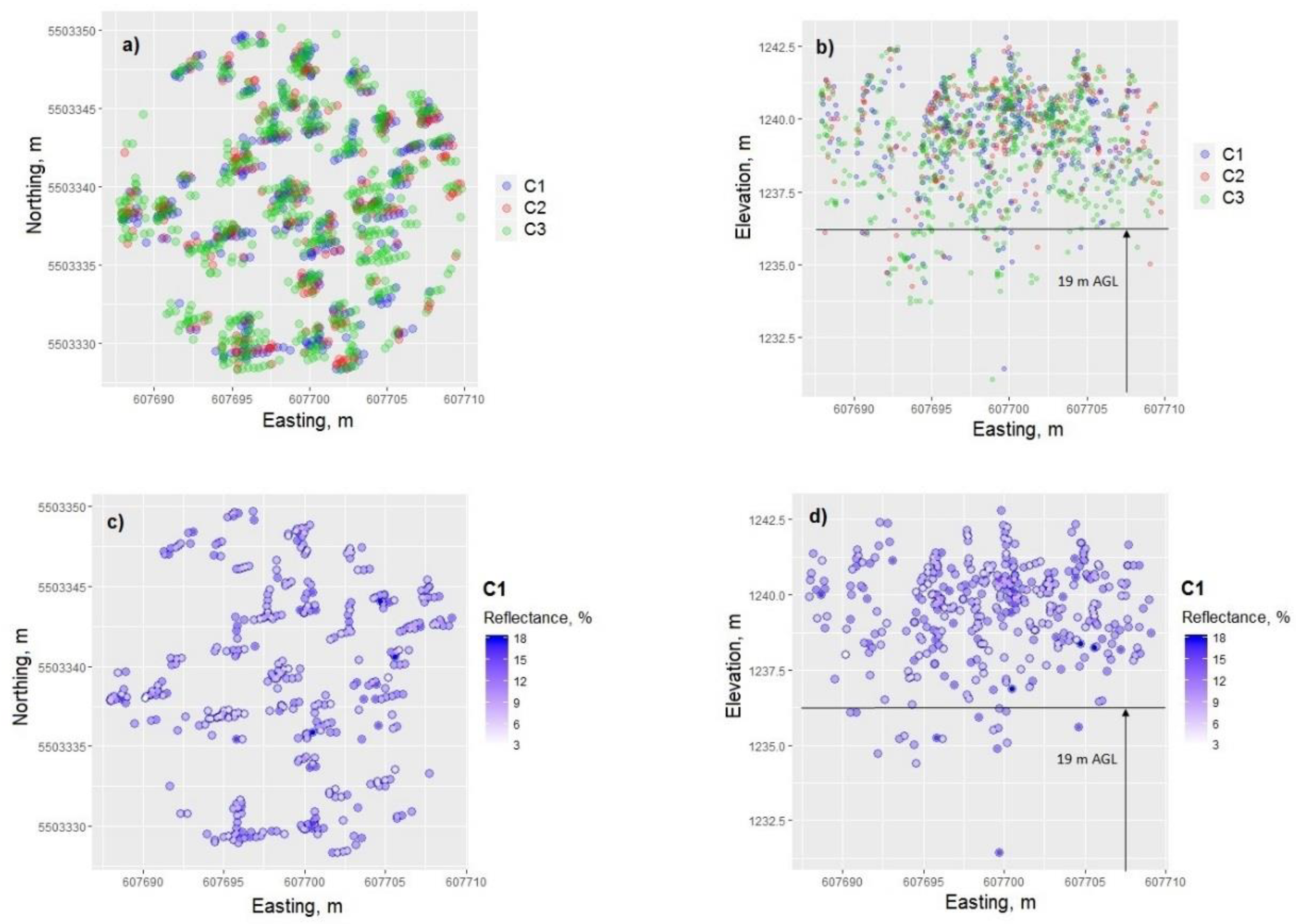
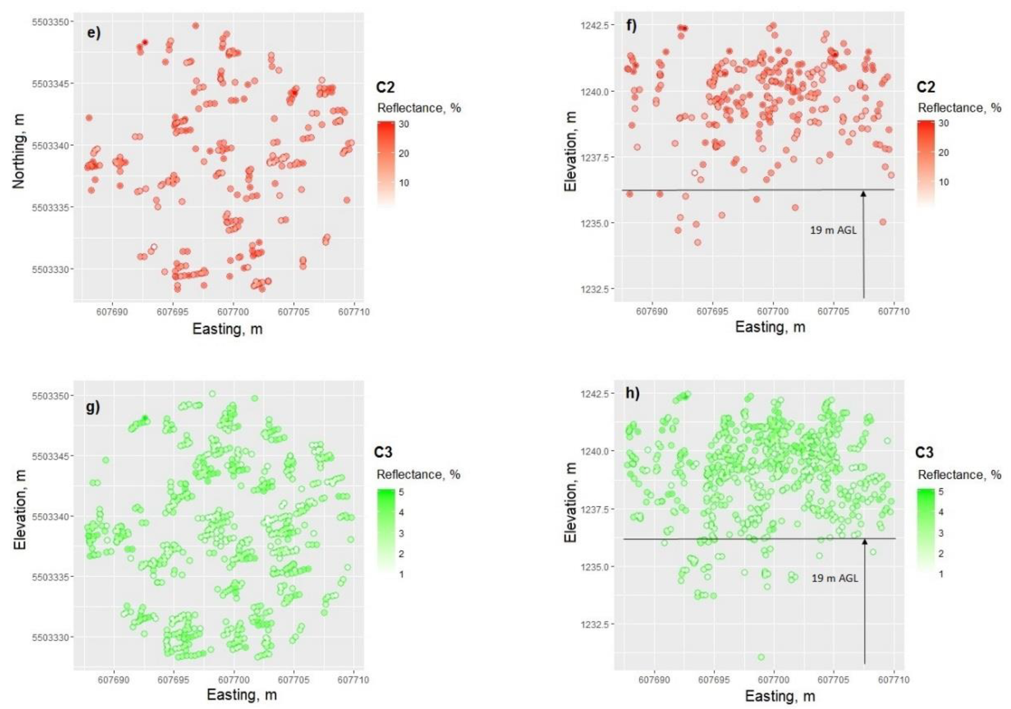
Top and side view of the established LP plot single returns derived from the spectral pseudo-reflectance values are shown in Figure 6 for each channel to illustrate available radiometric product after calibration.
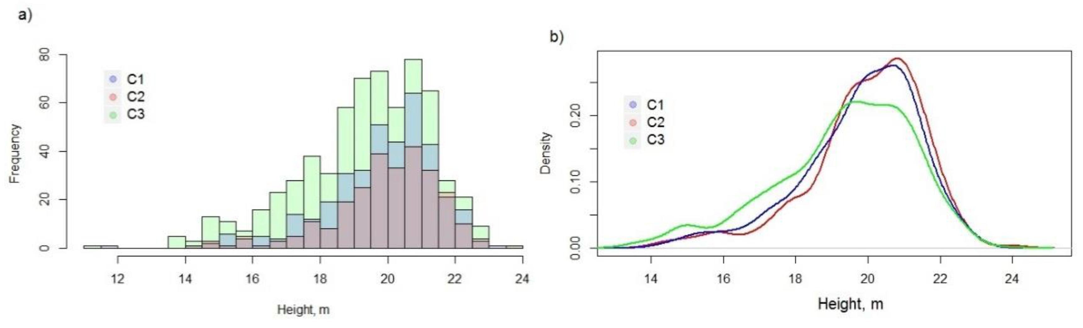
Height distribution histograms and their kernel densities for each channel for the established LP plot are presented in Figure 7. Table 9 shows results of Kolmogorov–Smirnov tests for two types of height distribution; one with a cut at 10 m above ground (there is no foliage below 10 m), and the second one with a cut at 19 m above ground. Height of 19 m represents approximate lowest level of full crown extent (Figure 6b,d,f,h), and was chosen on the descending slope of kernel density distributions of return heights from C1 and C2 at half-peak of the graph height (Figure 7b).
From Figure 5, Figure 6 and Figure 7, it is clear that there are more canopy single returns from C3 (N = 637) than C1 (N = 374), with the lowest number of single returns detected by C2 (N = 266). The difference is partly due to the different number of pulses emitted over the plot: 1712 for C3, 1492 for C2, and 1528 for C1. While the pulse repetition frequency (PRF) was the same for all channels, separation in tilt angle leads to a time separation (~1 s) in pulses hitting the same area, which results in a different point density due to aircraft attitude changes [32] mainly in pitch and heading (automatic roll compensation reduces the effect of aircraft attitude changes in roll). While different point density partially explains the variable number of single returns >10 m above ground for each channel, the ratio of single returns >10 m above ground to the number of emitted pulses is also different: 0.37 for C3, 0.18 for C2, and 0.24 for C1. Moreover, from the kernel density of height distributions for single returns >10 m above ground on Figure 7b, C3 samples lower parts of the canopy compared to C1 and C2 channels (p < 0.01 in Kolmogorov-Smirnov test, Table 9). C1 and C2 distributions are similar, and the Kolmogorov–Smirnov test produces a small D value (0.068) with corresponding large p (0.46), thus failing to reject the hypothesis that C1 and C2 channels sampled the same region of the canopy. These results corroborate similar observations reported in [4]. In addition, results from the below-canopy target experiment also show higher losses for C3 in comparison with C1 and C2 (Table 7). This effect can be caused by three main factors: Difference in the beam divergence, difference in the tilt angle, and difference in the spectral reflectance of vegetation. It is assumed, that the larger footprint and lower power density per unit area (irradiance) for C3, combined with the low reflectance values from vegetation at 532 nm leads to a higher proportion of undetected backscatter (i.e., not exceeding the signal to noise ratio of the detector) from within-canopy foliage. This systematically diminished ability for weak foliage pulse detection results in a higher proportion of single returns from vegetation for C3. A similar effect was reported in [32], where the observed proportion of split returns over vegetation reduced more rapidly with increasing survey altitude above ground for C3 relative to either C2 or C1. Higher tilt angle also increases the average path length through the canopy, which results in greater pulse attenuation. In the established plot (Figure 6 and Figure 7), the highest ratio of single return count >10 m to emitted pulse count is for C3 (tilt angle of 7°), the second is for C1 (3.5°), and the lowest is for C2 (at nadir). However, for single returns >19 m above ground, all three pairs C1 vs C2, C2 vs C3, and C1 vs C3, fail to reject the null hypothesis in the Kolmogorov–Smirnov test (p = 0.89, 0.33, and 0.19, respectively). Thus, we can establish that constructing vertical spectral vegetation index profiles may be feasible for the C1C2 pair through the whole vertical profile, and for pairs C2C3 and C1C3, for the upper foliage elements of the vegetation canopy (the top 4 m in the plot used in this study, for canopy between 19 and 23 m height).
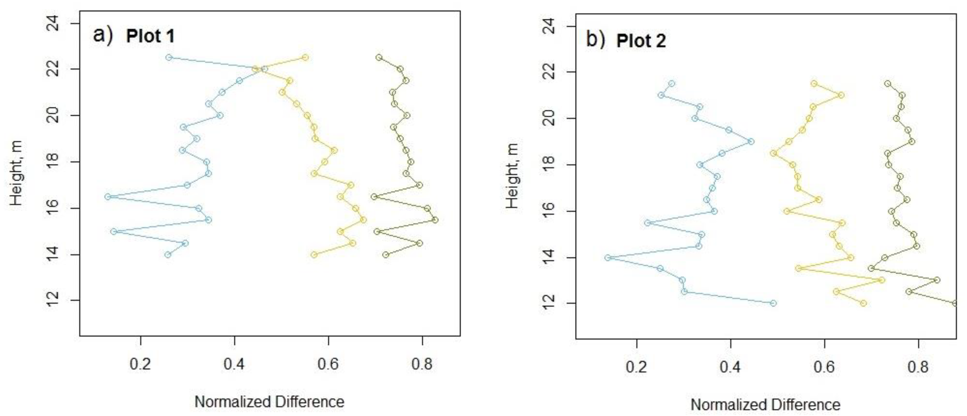
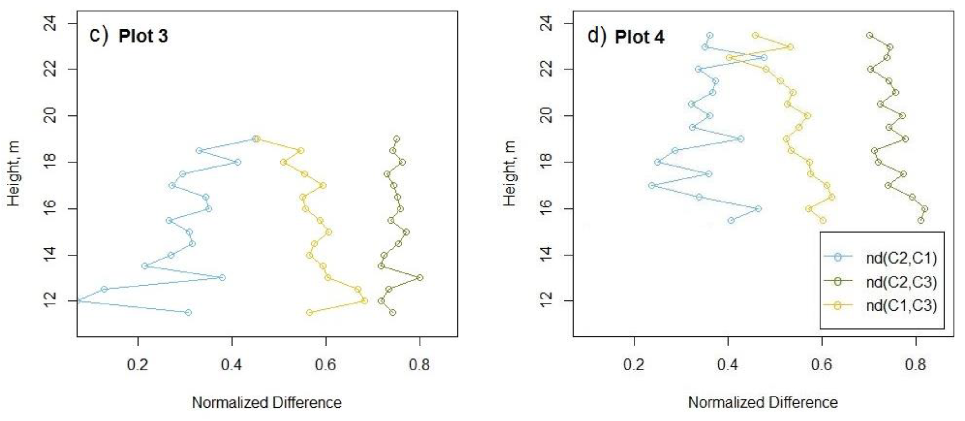
Vertical profiles of normalized differences for the LP plot canopy with the 0.5 m height bins are shown in Figure 8. Profiles start at 14 m above ground because there are insufficient single returns (Figure 8a) to derive indices below this canopy height.
From Figure 8, it can be seen that all three indices become noisy below a certain height (e.g., 18 m for Plot 1) due to decreasing single return counts as the crown extent thins. The lower voxel elements in two out of three indices are also noisy for the same reason. Also, the nδ(C2, C3) is almost constant through the canopy; in contrast, nδ(C2, C1) and nδ(C1, C3) have clear trends. The decrease of the water index nδ(C2, C1) with distance from the top of the canopy might be linked to the evapotranspiration characteristics of the vegetation and requires further investigation. The third index nδ(C1, C3) resembles the combined behavior of the first two indices because it can be re-written as their combination. The resulting nδ(C2, C3) on Figure 8 is comparable with the modeled response of ms lidar in [20] and lab measurement results in [21]. However, for comparing individual canopy SVI profiles, segmentation algorithms [38,39] should be applied to construct active SVIs for individual trees. Individual trees SVIs profile might be useful for tree species classification and forest health monitoring.
3.6. Maps and Vertical Profile of Spectral Vegetation Indices
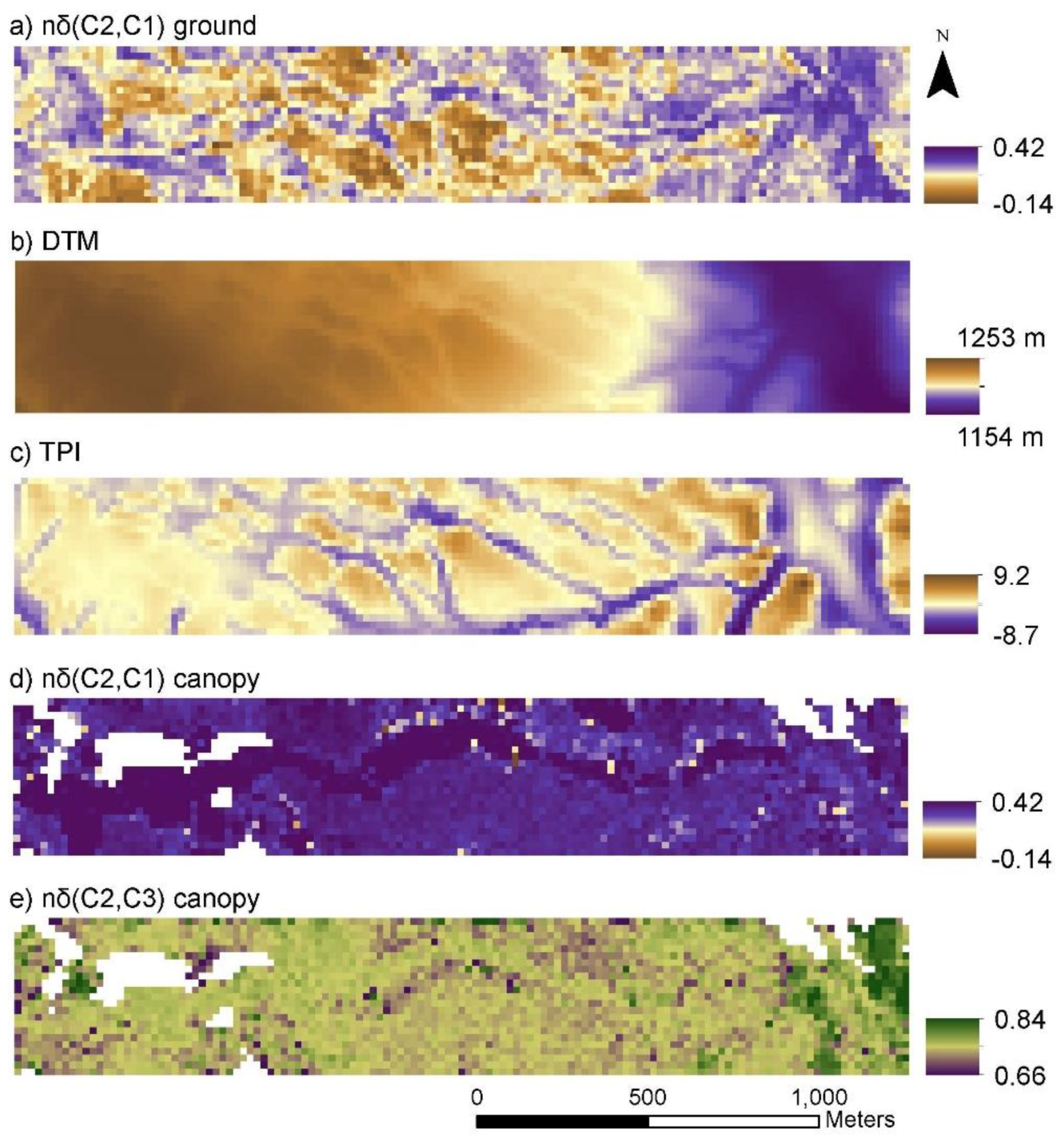
The map of the ground-level nδ(C2, C1) in Figure 9a shows distinct patterns across the surface (lower values of the index). When compared to the DTM (Figure 9b) and TPI (Figure 9c, note inverted color ramp), it illustrates some visible spatial correspondence with hills and local valleys (R = –0.35, Pearson correlation coefficient for the TPI map). This may further suggest that the ground-level nδ(C2, C1) was influenced by the wetness of the ground below forest canopy. The canopy nδ(C2, C1) map on Figure 9d exhibits higher values than at ground level (mean values 0.36 and 0.15) and there are generally higher values along the road corridor of bare ground and short vegetation (see Figure 2 for reference) between forest covered hills. The nδ(C2, C3) map of the canopy (Figure 9e) shows relatively high values (mean 0.75) across the whole AOI with a distinct area of higher values in the eastern part depicting a hill with young aspen stands.
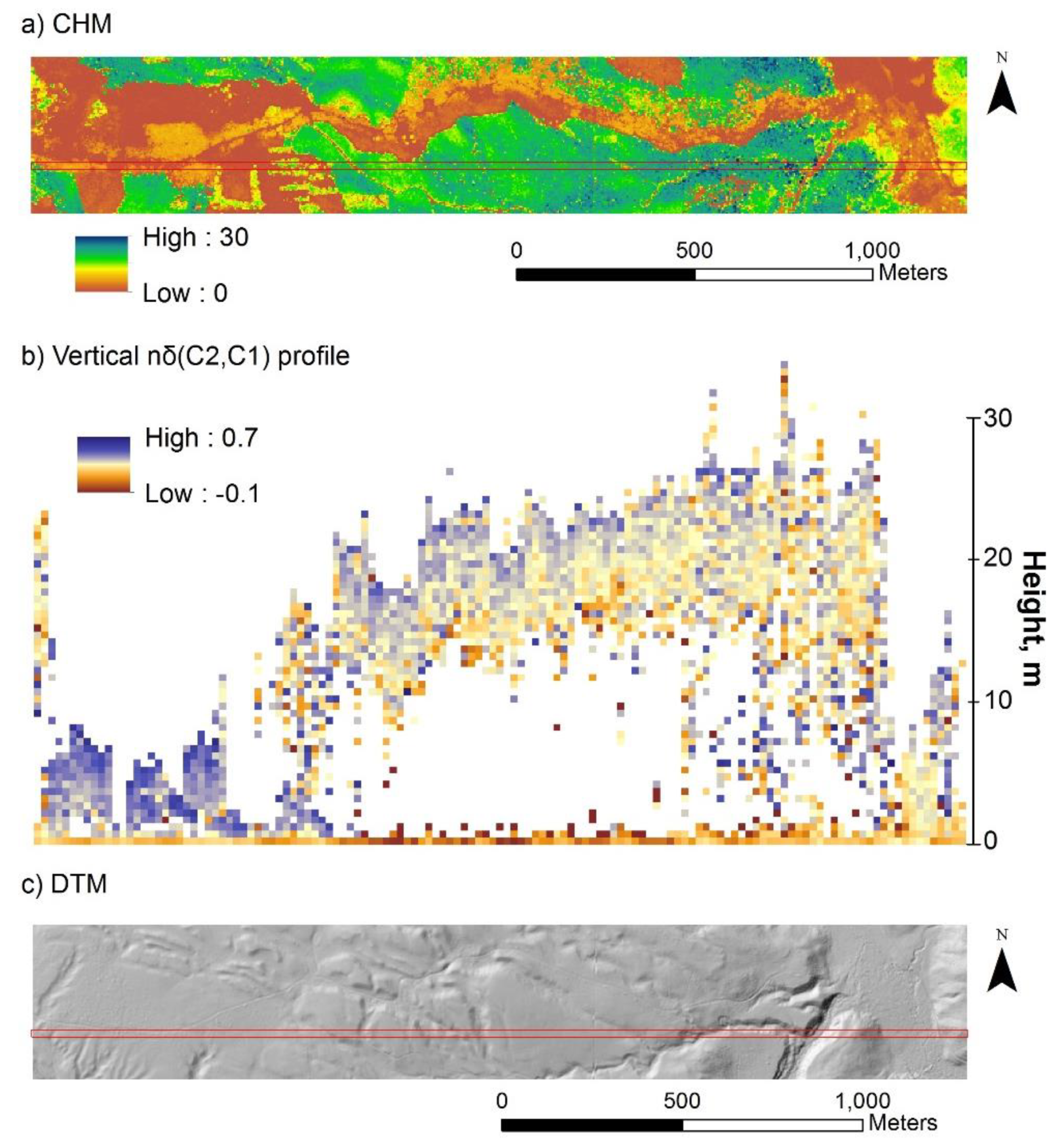
The voxel profile transect of nδ(C2, C1) in Figure 10b illustrates a distinct vertical gradient of the index through the canopy. Moreover, the transect illustrates the spatial variation in index values along the transect and its gradient from younger stands (west end), to mature LP stands (center portion) to the more complex understory on the hill slopes and valley wetland area (east end). Thus, the vertical profile transect in Figure 10b illustrates the potential of plot level voxelization and 3D mapping of active spectral vegetation indices.
4. Conclusions
Radiometric calibration targets help bridge the gap between ms lidar products and available spectral signature libraries. The low-cost diffuse reflection coating [28] is an acceptable operational substitute to Spectralon® (Labspere Inc., North Sutton, NH, USA) panels allowing investigation of complex lidar backscatter without being cost-prohibitive and also allows custom calibration targets. The algorithm described by Equation (1), is promising; however, it should be combined with an additional model of energy losses in the canopy, and an explanation of the results of the lifted target experiment may be a first step in creating such a model. Vertical SVIs for the canopy can be calculated from corrected Titan DNs up to a certain penetration depth; in our study plot up to 4 m. Canopy vertical profile of normalized difference of C2 and C3 for an LP plot looks similar to predicted profiles of NDVI by modeling and lab measurements [20,21]. It is possible to generate vertical profiles of the normalized difference of C1 and C2 from the Titan sensor from the top of the canopy to the ground, providing there are enough single returns in each height bin, and ground surface remains in the lowest bin for the spatial extent being sampled (i.e., terrain slope does not force ground surface into multiple height bins). The potential for plot level voxelization and 3D mapping of active spectral vegetation indices was demonstrated with a vertical profile transect of nδ(C2, C1) across the study area.
Future work could consider development of recipes for coatings with lower spectral reflectance values, down to 5%. Targets covered with such a coating would allow the prediction of receiver response to low values of lidar backscatter and enable modeling of sensor Signal to Noise Ratio (SNR) for analyzing volumetric backscatter of the canopy. Additional analysis of energy losses in the lifted target experiment may help to understand signal attenuation in canopy foliage and allow derivation of spectral reflectance and estimation of illuminated areas from split returns. The new methodology of constructing voxel-based active 3D SVIs on a stand level brings new potential to classification, comparison, and change monitoring in forest and wetland environments. However, to be able to compare active 3D SVIs through time and space, more research is needed into standardization. In addition, segmentation of the lidar point cloud from the forest stand into individual trees, if successful, could provide a means to construct vertical SVI profiles for each detected tree allowing the enhancement of species classification and forest health monitoring with ms lidar.
Author Contributions
Conceptualization, C.H. and M.O.; methodology, C.H., C.C., and M.O.; software, C.H.; validation, C.C. and M.O..; formal analysis, M.O.; investigation, M.O. and C.H.; resources, C.H. and C.C.; data curation, C.H. and M.O.; writing—original draft preparation, M.O.; writing—review and editing, C.H., C.C., and M.O.; visualization, M.O.; supervision, C.H.; project administration, C.H.; funding acquisition, C.H. and M.O.
Funding
Okhrimenko acknowledges funding from Alberta Innovates Technology Futures. Hopkinson acknowledges funding from Canada Foundation for Innovation, NSERC, and Alberta Economic Development & Trade.
Acknowledgments
Teledyne Optech is gratefully acknowledged for providing the ms lidar sensor for the airborne missions along with Mike Sitar and Paul LaRocque for their constant help and support. Peter Kennedy is acknowledged for help in validation of radiometric targets spectral reflectance. Zhouxin Xi, David McCaffrey, Reed Parsons, and Laura Chasmer are acknowledged for providing field support. Locke Spencer, Derek Peddle, and Craig Mahoney acknowledged for useful discussions and friendly critique.
Conflicts of Interest
The authors declare no conflict of interest.
References
- Vosselman, G.; Maas, H. Airborne and Terrestrial Laser Scanning; CRC Press: Boca Raton, FL, USA, 2010. [Google Scholar]
- Bannari, A.; Morin, D.; Bonn, F.; Huete, A.R. A review of vegetation indices. Indices. Remote Sens. Rev. 1995, 13, 95–120. [Google Scholar] [CrossRef]
- Hancock, S.; Lewis, P.; Foster, M.; Disney, M.; Muller, J. Measuring forests with dual wavelength lidar: A simulation study over topography. Agric. For. Meteorol. 2012, 161, 123–133. [Google Scholar] [CrossRef] [Green Version]
- Hopkinson, C.; Hopkinson, C.; Chasmer, L.; Gynan, C.; Mahoney, C.; Sitar, M. Multisensor and Multispectral LiDAR Characterization and Classification of a Forest Environment. Can. J. Remote Sens. 2016, 42, 501–520. [Google Scholar] [CrossRef]
- Wallace, A.; Nichol, C.; Woodhouse, I. Recovery of Forest Canopy Parameters by Inversion of Multispectral LiDAR Data. Remote Sens. 2012, 4, 509–531. [Google Scholar] [CrossRef] [Green Version]
- Holmgren, J.; Nilsson, M.; Olsson, H. Simulating the effects of lidar scanning angle for estimation of mean tree height and canopy closure. Can. J. Remote Sens. 2003, 29, 623–632. [Google Scholar] [CrossRef]
- Hopkinson, C.; Chasmer, L.; Hall, R.J. The uncertainty in conifer plantation growth prediction from multi-temporal lidar datasets. Remote Sens. Environ. 2008, 112, 1168–1180. [Google Scholar] [CrossRef]
- Stoker, J.M.; Cochrane, M.A.; Roy, D.P. Integrating Disparate Lidar Data at the National Scale to Assess the Relationships between Height Above Ground, Land Cover and Ecoregions. Photogramm. Eng. Remote Sens. 2014, 80, 59–70. [Google Scholar] [CrossRef]
- Mahoney, C.; Hopkinson, C.; Held, A.; Simard, M. Continental-Scale Canopy Height Modeling by Integrating National, Spaceborne, and Airborne LiDAR Data. Can. J. Remote Sens. 2016, 42, 574–590. [Google Scholar] [CrossRef]
- Yu, X.W.; Hyyppä, J.; Kukko, A.; Maltamo, M.; Kaartinen, H. Change detection techniques for canopy height growth measurements using airborne laser scanner data. Photogramm. Eng. Remote Sens. 2006, 72, 1339–1348. [Google Scholar] [CrossRef]
- Bater, C.W.; Coops, N.; Gergel, S.E.; LeMay, V.; Collins, D. EEstimation of standing dead tree class distributions in northwest coastal forests using lidar remote sensing. Can. J. For. Res.-Rev. Can. De Rech. For. 2009, 39, 1080–1091. [Google Scholar] [CrossRef]
- Donoghue, D.N.M.; Watt, P.; Cox, N.J.G.; Wilson, D.J. Remote sensing of species mixtures in conifer plantations using LiDAR height and intensity data. Remote Sens. Environ. 2007, 110, 509–522. [Google Scholar] [CrossRef]
- Okhrimenko, M.; Coburn, C.; Hopkinson, C. Investigating Multi-Spectral Lidar Radiometry: An Overview of the Experimental Framework. In Proceedings of the IGARSS 2018–2018 IEEE International Geoscience and Remote Sensing Symposium, Valencia, Spain, 23–27 July 2018; pp. 8745–8748. [Google Scholar]
- Karila, K.; Matikainen, L.; Puttonen, E.; Hyyppä, J. Feasibility of Multispectral Airborne Laser Scanning Data for Road Mapping. Ieee Geosci. Remote Sens. Lett. 2017, 14, 294–298. [Google Scholar] [CrossRef]
- Matikainen, L.; Karila, K.; Hyyppä, J.; Litkey, P.; Puttonen, E.; Ahokas, E. Object-based analysis of multispectral airborne laser scanner data for land cover classification and map updating. Isprs J. Photogramm. Remote Sens. 2017, 128, 298–313. [Google Scholar] [CrossRef]
- Morsy, S.; Shaker, A.; El-Rabbany, A. Multispectral LiDAR Data for Land Cover Classification of Urban Areas. Sensors 2017, 17, 958. [Google Scholar] [CrossRef]
- Morsy, S.; Shaker, A.; El-Rabbany, A.; LaRocque, P.E. Airborne Multispectral Lidar Data for Land-Cover Classification and Land/Water Mapping Using Different Spectral Indexes. ISPRS Ann. Photogramm. Remote Sens. Spat. Inf. Sci. 2016, 3, 217–224. [Google Scholar] [CrossRef]
- Budei, B.C.; St-Onge, B.; Hopkinson, C.; Audet, F. Identifying the genus or species of individual trees using a three-wavelength airborne lidar system. Remote Sens. Environ. 2018, 204, 632–647. [Google Scholar] [CrossRef]
- Hancock, S.; Gaulton, R.; Danson, F.M. Angular Reflectance of Leaves With a Dual-Wavelength Terrestrial Lidar and Its Implications for Leaf-Bark Separation and Leaf Moisture Estimation. IEEE Trans. Geosci. Remote Sens. 2017, 55, 3084–3090. [Google Scholar] [CrossRef] [Green Version]
- Morsdorf, F.; Nichol, C.; Malthus, T.; Woodhouse, I. Assessing forest structural and physiological information content of multi-spectral LiDAR waveforms by radiative transfer modelling. Remote Sens. Environ. 2009, 113, 2152–2163. [Google Scholar] [CrossRef] [Green Version]
- Woodhouse, I.H.; Nichol, C.; Sinclair, P.; Jack, J.; Morsdorf, F.; Malthus, T.; Patenaude, G. A Multispectral Canopy LiDAR Demonstrator Project. Ieee Geosci. Remote Sens. Lett. 2011, 8, 839–843. [Google Scholar] [CrossRef]
- Yan, W.Y.; Shaker, A.; Habib, A.; Kersting, A.P. Improving classification accuracy of airborne LiDAR intensity data by geometric calibration and radiometric correction. Isprs J. Photogramm. Remote Sens. 2012, 67, 35–44. [Google Scholar] [CrossRef]
- Kaasalainen, S.; Hyyppä, H.; Kukko, A.; Litkey, P. Radiometric Calibration of LIDAR Intensity With Commercially Available Reference Targets. Ieee Trans. Geosci. Remote Sens. 2009, 47, 588–598. [Google Scholar] [CrossRef]
- Vain, A.; Kaasalainen, S.; Pyysalo, U.; Krooks, A.; Litkey, P. Use of Naturally Available Reference Targets to Calibrate Airborne Laser Scanning Intensity Data. Sensors 2009, 9, 2780–2796. [Google Scholar] [CrossRef] [PubMed]
- Vain, A.; Yu, X.; Kaasalainen, S.; Hyyppä, J. Correcting Airborne Laser Scanning Intensity Data for Automatic Gain Control Effect. Ieee Geosci. Remote Sens. Lett. 2010, 7, 511–514. [Google Scholar] [CrossRef]
- Milenkovic, M. Total canopy transmittance estimated from small-footprint, full-waveform airborne LiDAR. Isprs J. Photogramm. Remote Sens. 2017, 128, 61–72. [Google Scholar] [CrossRef]
- Kashani, A.G.; Olsen, M.J.; Parrish, C.; Wilson, N. A Review of LIDAR Radiometric Processing: From Ad Hoc Intensity Correction to Rigorous Radiometric Calibration. Sensors 2015, 15, 28099–28128. [Google Scholar] [CrossRef] [PubMed] [Green Version]
- Noble, S.D.; Boeré, A.; Kondratowicz, T.; Crowe, T.G.; Brown, R.B.; Naylor, D.A. Characterization of a low-cost diffuse reflectance coating. Can. J. Remote Sens. 2008, 34, 68–76. [Google Scholar] [CrossRef]
- Vain, A.; Kaasalainen, S.; Hyyppä, J.; Ahokas, E. Calibration of laser scanning intensity data using brightness targets. The method developed by the Finnish Geodetic Institute. Geod. Ir Kartogr. 2009, 35, 77–81. [Google Scholar] [CrossRef]
- Beaty, C.B. The Landscapes of Southern Alberta; The University of Lethbridge: Lethbridge, AL, Canada, 1975. [Google Scholar]
- Fernandez-Diaz, J.C.; Carter, W.; Glennie, C.; Shrestha, R.; Pan, Z.; Ekhtari, N.; Singhania, A.; Hauser, D.; Singhania, A. Capability Assessment and Performance Metrics for the Titan Multispectral Mapping Lidar. Remote Sens. 2016, 8, 936. [Google Scholar] [CrossRef]
- Okhrimenko, M.; Hopkinson, C. The consistency of uncalibrated multispectral lidar vegetation indices at different altitudes. Remote Sens. 2019, 11, 1531. [Google Scholar] [CrossRef]
- Yan, W.Y.; Shaker, A. Airborne LiDAR intensity banding: Cause and solution. Isprs J. Photogramm. Remote Sens. 2018, 142, 301–310. [Google Scholar] [CrossRef]
- CSRS. PPP Service. 2017. Available online: https://webapp.geod.nrcan.gc.ca/geod/tools-outils/ppp.php?locale=en (accessed on 15 September 2017).
- Kokaly, R.F.; Despain, D.G.; Clark, R.N.; Livo, K.E. Mapping vegetation in Yellowstone National Park using spectral feature analysis of AVIRIS data. Remote Sens. Environ. 2003, 84, 437–456. [Google Scholar] [CrossRef] [Green Version]
- Kokaly, R.F.; Clark, R.N.; Swayze, G.A.; Livo, K.E.; Hoefen, T.M.; Pearson, N.C.; Wise, R.A.; Benzel, W.M.; Lowers, H.A.; Driscoll, R.L.; et al. Lodgepole-Pine LP-Needles-1. In USGS Spectral Library, Version 7: U.S. Geological Survey Data Series 1035; 2017; p. 61. [Google Scholar] [CrossRef]
- Korpela, I. Acquisition and evaluation of radiometrically comparable multi-footprint airborne LiDAR data for forest remote sensing. Remote Sens. Environ. 2017, 194, 414–423. [Google Scholar] [CrossRef] [Green Version]
- Koch, B.; Kattenborn, T.; Straub, C.; Vauhkonen, J. Segmentation of Forest to Tree Objects, Forestry Applications of Airborne Laser Scanning: Concepts and Case Studies; Springer: Heidelberg, Germany, 2014; Volume 27, pp. 89–112. [Google Scholar]
- Okhrimenko, M.; Grabarnik, P. Segmentation of LiDAR points in forest environment based on unidirected graphs. In Proceedings of the VII International Conference Mathematical Biology and Bioinformatics, Puschino, Russia, 14–19 October 2016. [Google Scholar]
Figure 1.
Photos of the radiometric calibration targets (made from 8′ by 4′ plywood). Photos (a), (b,c) are an open target, lifted target, and below-canopy target, respectively. Photos (d,f) illustrate corresponding transparency of the Lodgepole Pine foliage above the target and transparency of the lifted target.

Figure 2.
(a) Map of Canada with highlighted Province of Saskatchewan and indicated Cypress Hills Interprovincial Park. (b) Area of interest (AOI) inside Cypress Hills Interprovincial Park colorized by RGB passive imagery. The lodgepole pine (LP) stand and plots (established and random virtual) are depicted inside the AOI.

Figure 3.
Illustration of the C2 footprints (at 1/e2) on the open target.

Figure 4.
Spectral reflectance curve for the constructed targets.

Figure 5.
Left to right: C1, C2, and C3 spectral reflectance (in %) histograms for single returns of the canopy (>10 m above ground) of the established Lodgpole Pine plot (Plot 1) of 11.3 m radii.
Figure 5.
Left to right: C1, C2, and C3 spectral reflectance (in %) histograms for single returns of the canopy (>10 m above ground) of the established Lodgpole Pine plot (Plot 1) of 11.3 m radii.

Figure 6.
(a,b) All channel single returns for the established LP plot canopy combined in one image without intensity information. (c–h) Single-return intensities coded with color for the LP plot 1 canopy for all three channels. Cutoff line at 19 m above ground is shown by black horizontal line in (b,d,f,h).


Figure 7.
Histograms of height distribution of single returns for C1, C2, and C3 over LP plot (a), and corresponding kernel densities (b).
Figure 7.
Histograms of height distribution of single returns for C1, C2, and C3 over LP plot (a), and corresponding kernel densities (b).

Figure 8.
LP plot-level canopy vertical spectral vegetation indices (SVIs) derived from spectral pseudo-reflectance values for plots in Figure 2b. (a) Plot 1; (b) Plot 2; (c) Plot 3; (d) Plot 4.
Figure 8.
LP plot-level canopy vertical spectral vegetation indices (SVIs) derived from spectral pseudo-reflectance values for plots in Figure 2b. (a) Plot 1; (b) Plot 2; (c) Plot 3; (d) Plot 4.


Figure 9.
AOI maps of (a) ground nδ(C2,C1), (b) DTM (Digital Terrain Model), (c) TPI (Topographic Position Index), (d) canopy nδ(C2,C1), and (e) canopy nδ(C2,C3). Note, the AOI covers the same area as presented in Figure 2. Blank (white) pixels represent open areas of insufficient data for canopy SVI generation. Note inverted color ramp in (a,d) vs. (b,c).

Figure 10.
(a) Canopy Height Model (CHM) with a 20 m wide cross-section (in red) used to extract vertical profile data; (b) vertical nδ(C2,C1) profile, height is scaled 40× relative ground distance; (c) DTM showing cross-section location (in red).
Figure 10.
(a) Canopy Height Model (CHM) with a 20 m wide cross-section (in red) used to extract vertical profile data; (b) vertical nδ(C2,C1) profile, height is scaled 40× relative ground distance; (c) DTM showing cross-section location (in red).


Table 1.
Titan sensor laser characteristics and footprint diameter at 600 m AGL.
| Channel | Wavelength | Forward Tilt | Divergence (1/e) | Divergence (1/e)2 | Footprint Diameter (1/e)2 at 600 m |
|---|---|---|---|---|---|
| C1 | 1550 nm | 3.5° | 0.35 mrad | 0.5 mrad | 30 cm |
| C2 | 1064 nm | 0.0° | 0.35 mrad | 0.5 mrad | 30 cm |
| C3 | 532 nm | 7.0° | 0.7 mrad | 1.0 mrad | 60 cm |
Table 2.
Point density per m−2 of forest covered compared to open area (second value) for one flight line averaged over 11.3 m radii plot areas for each channel.
Table 2.
Point density per m−2 of forest covered compared to open area (second value) for one flight line averaged over 11.3 m radii plot areas for each channel.
| Channel | C3 | C2 | C1 |
|---|---|---|---|
| Wavelength | 532 nm | 1064 nm | 1550 nm |
| Point density | ~4.5/2.7 | ~6.8/2.9 | ~5.8/2.9 |
Table 3.
Values of spectral reflectance for wavelengths corresponding to Titan measured by ASD (20 samples). RMSE values in brackets.
Table 3.
Values of spectral reflectance for wavelengths corresponding to Titan measured by ASD (20 samples). RMSE values in brackets.
| Wavelength | C3 (532 nm) | C2 (1064 nm) | C1 (1550 nm) |
|---|---|---|---|
| Spectral reflectance % | 95.5 (0.1) | 95.0 (0.5) | 90.5 (0.9) |
Table 4.
Values of DNs corresponding to 100% spectral reflectance, normalized to 600 m and calculated values of spectral reflectance from the cross line. SD values and number of measurements (SD | N) are given in brackets.
Table 4.
Values of DNs corresponding to 100% spectral reflectance, normalized to 600 m and calculated values of spectral reflectance from the cross line. SD values and number of measurements (SD | N) are given in brackets.
| Observations | C3 (532 nm) | C2 (1064 nm) | C1 (1550 nm) |
|---|---|---|---|
| DN normalized to 100% spectral reflectance (600 m) | 3068 (116 | 3) | 3151 (52 | 5) | 3267 (145 | 6) |
| Cross line spectral reflectance validation % | 93.4 (1.8 | 4) | 96.4 (2.9 | 5) | 91.0 (1.4 | 5) |
Table 5.
Comparison of spectral pseudo-reflectance derived from Titan single returns (SD in brackets) for LP stand in Cypress Hills to spectral reflectance data derived from different locations from AVIRIS, AISA Dual, and ASD, and calculated two simple ratios ( and ). p-values of two-sample Mann-Whitney test comparing Titan’s spectral pseudo-reflectance and spectral ratios vs. AVIRIS and AISA Dual data are presented.
| Observations | Pixel Size | N | C3 (532 nm) | C2 (1064 nm) | C1 (1550 nm) | ||
|---|---|---|---|---|---|---|---|
| Titan All LP, % | 15 m | 150 | 3.4 (0.5) | 27.7 (3.3) | 18.2 (2.8) | 0.12 (0.01) | 0.66 (0.07) |
| Vs. AVIRIS | p < 0.05 | p < 0.05 | p < 0.05 | p < 0.05 | p < 0.05 | ||
| Vs. Aisa Dual | p < 0.05 | p < 0.05 | p < 0.05 | p < 0.05 | p < 0.05 | ||
| Titan Canopy LP, % | 15 m | 150 | 2.5 (0.1) | 17.6 (0.7) | 8.4 (0.3) | 0.14 (0.01) | 0.48 (0.02) |
| Vs. AVIRIS | p = 0.09 | p < 0.05 | p = 0.51 | p = 1 | p = 0.39 | ||
| Vs. Aisa Dual | p < 0.05 | p < 0.05 | p < 0.05 | p < 0.05 | p < 0.05 | ||
| AVIRIS YNP-LP1, % | 15 m | 4 | 2.3 (0.5) | 15.3 (0.9) | 8.0 (1.4) | 0.15 (0.02) | 0.52 (0.07) |
| AISA Dual Pines, % | 2 m | 37 | 5.5 (0.7) | 31.5 (5.4) | 10.7 (2.8) | 0.18 (0.02) | 0.34 (0.08) |
| ASD LP, % | * | 1 | 19.2 (5.0) | 67.1 (2.3) | 38.4 (3.9) | 0.28 | 0.57 |
Table 6.
Lifted target calibrated digital numbers (DNs) from double returns (first and last) with the percentage of the sum relative to the open target DN for each channel. The average loss in comparison to the open target is shown in the bottom row.
Table 6.
Lifted target calibrated digital numbers (DNs) from double returns (first and last) with the percentage of the sum relative to the open target DN for each channel. The average loss in comparison to the open target is shown in the bottom row.
| Channel | C3 (532 nm) | C2 (1064 nm) | C1 (1550 nm) | ||||||
|---|---|---|---|---|---|---|---|---|---|
| Double returns observations | first | last | first | last | first | last | |||
| 953 | 1381 | 79.7% | 2162 | 430 | 86.6% | 1369 | 1277 | 84.4% | |
| 1265 | 1001 | 77.3% | 1224 | 1240 | 82.3% | 1344 | 1198 | 81.0% | |
| 1333 | 824 | 73.6% | 1314 | 1192 | 83.7% | 1778 | 1101 | 91.8% | |
| 1776 | 816 | 86.6% | |||||||
| Average loss | 23.1% | 15.2% | 14.3% | ||||||
Table 7.
Below-canopy single return DNs vs. open target DNs and the corresponding loss in intensity values in percentage. DN values were normalized to a 600 m range and corrected with the cosine of incidence angle. Only one hit (N = 1) for each channel was detected for the below-canopy target.
Table 7.
Below-canopy single return DNs vs. open target DNs and the corresponding loss in intensity values in percentage. DN values were normalized to a 600 m range and corrected with the cosine of incidence angle. Only one hit (N = 1) for each channel was detected for the below-canopy target.
| Observations | C3 (532 nm) | C2 (1064 nm) | C1 (1550 nm) |
|---|---|---|---|
| Below-canopy target single return hit, DN | 942 | 2838 | 3054 |
| Open target, DN | 2930 | 2994 | 3136 |
| Loss | 68% | 5% | 3% |
Table 8.
Canopy spectral reflectance derived from below-canopy return responses and illuminated area on the below-canopy radiometric calibration target as a percentage of the footprint area at nadir.
Table 8.
Canopy spectral reflectance derived from below-canopy return responses and illuminated area on the below-canopy radiometric calibration target as a percentage of the footprint area at nadir.
| Channel | Target Hit | First return Backscatter | Intermediate Return Backscatter | ||
|---|---|---|---|---|---|
| C1 | 1 | 8.5% | 6.0% | 2.5% | 1% |
| 2 | 12.0% | 12.0% | 64% | ||
| 3 | 12.1% | 9.7% | 2.4% | 3% | |
| 4 | 18.1% | 12.1% | 6.0% | 29% | |
| 5 | 11.4% | 3.9% | 7.5% | 57% | |
| C2 | 1 | 21.8% | 21.8% | 54% | |
| C3 | 1 | 2.6% | 1.3% | 1.3% | 11% |
| 2 | 2.2% | 2.2% | 8% | ||
| 3 | 2.4% | 1.3% | 1.1% | 20% | |
| 4 | 3.1% | 3.1% | 18% | ||
| 5 | 1.4% | 1.4% | 27% | ||
| 6 | 1.9% | 1.9% | 29% |
Table 9.
Results of Kolmogorov-Smirnov test D values (p-value in brackets) for returns higher than 10 m above ground (in the upper-right), and returns higher than 19 m above ground (in the lower-left).
Table 9.
Results of Kolmogorov-Smirnov test D values (p-value in brackets) for returns higher than 10 m above ground (in the upper-right), and returns higher than 19 m above ground (in the lower-left).
| C1 | C2 | C1 | |
|---|---|---|---|
| C1 | - | 0.068 (0.46) | 0.138 (<0.01) |
| C2 | 0.053 (0.89) | - | 0.173 (<0.01) |
| C3 | 0.085 (0.19) | 0.081 (0.33) | - |
© 2019 by the authors. Licensee MDPI, Basel, Switzerland. This article is an open access article distributed under the terms and conditions of the Creative Commons Attribution (CC BY) license (http://creativecommons.org/licenses/by/4.0/).
Share and Cite
MDPI and ACS Style
Okhrimenko, M.; Coburn, C.; Hopkinson, C. Multi-Spectral Lidar: Radiometric Calibration, Canopy Spectral Reflectance, and Vegetation Vertical SVI Profiles. Remote Sens. 2019, 11, 1556. https://0-doi-org.brum.beds.ac.uk/10.3390/rs11131556
AMA Style
Okhrimenko M, Coburn C, Hopkinson C. Multi-Spectral Lidar: Radiometric Calibration, Canopy Spectral Reflectance, and Vegetation Vertical SVI Profiles. Remote Sensing. 2019; 11(13):1556. https://0-doi-org.brum.beds.ac.uk/10.3390/rs11131556
Chicago/Turabian StyleOkhrimenko, Maxim, Craig Coburn, and Chris Hopkinson. 2019. "Multi-Spectral Lidar: Radiometric Calibration, Canopy Spectral Reflectance, and Vegetation Vertical SVI Profiles" Remote Sensing 11, no. 13: 1556. https://0-doi-org.brum.beds.ac.uk/10.3390/rs11131556
Note that from the first issue of 2016, this journal uses article numbers instead of page numbers. See further details here.