Article

Semi-Automatic Identification and Pre-Screening of Geological–Geotechnical Deformational Processes Using Persistent Scatterer Interferometry Datasets

by
Roberto Tomás
1,*,
José Ignacio Pagán
1,
José A. Navarro
2,
Miguel Cano
1,
José Luis Pastor
1,
Adrián Riquelme
1,
María Cuevas-González
2,
Michele Crosetto
2,
Anna Barra
2,
Oriol Monserrat
2,
Juan M. Lopez-Sanchez
3,
Alfredo Ramón
4,
Salvador Ivorra
1,
Matteo Del Soldato
5,
Lorenzo Solari
5,
Silvia Bianchini
5,
Federico Raspini
5,
Fabrizio Novali
6,
Alessandro Ferretti
6,
Mario Costantini
7,
Francesco Trillo
7,
Gerardo Herrera
8,9 and
Nicola Casagli
5
add Show full author list remove Hide full author list
1
Departamento de Ingeniería Civil, Universidad de Alicante, P.O. Box 99, 03080 Alicante, Spain
2
Centre Tecnològic de Telecomunicacions de Catalunya (CTTC/CERCA), Geomatics Division, Av. Gauss, 7 08860 Castelldefels, Spain
3
Instituto Universitario de Investigación Informática, Universidad de Alicante, P.O. Box 99, 03080 Alicante, Spain
4
Sistema de Información Geográfica de la Universidad de Alicante (SIGUA), Universidad de Alicante, P.O. Box 99, 03080 Alicante, Spain
5
Earth Sciences Department, University of Florence, Via La Pira, 4, 50121 Firenze, Italy
6
TRE-Altamira, Via di Ripa Ticinese, 79, 20143 Milan, Italy
7
e-GEOS—An Italian Space Agency/Telespazio Company, Via Tiburtina, 965, 00156 Rome, Italy
8
Geohazards InSAR Laboratory and Modeling Group, Instituto Geológico y Minero de España (IGME), C/ Alenza 1, 28003 Madrid, Spain
9
Earth Observation and Geohazards Expert Group (EOEG), EuroGeoSurveys, the Geological Surveys of Europe, Rue Joseph II, 36–38, 1000 Brussels, Belgium
*
Author to whom correspondence should be addressed.
Remote Sens. 2019, 11(14), 1675; https://0-doi-org.brum.beds.ac.uk/10.3390/rs11141675
Submission received: 24 May 2019 / Revised: 4 July 2019 / Accepted: 12 July 2019 / Published: 14 July 2019

Abstract

:
This work describes a new procedure aimed to semi-automatically identify clusters of active persistent scatterers and preliminarily associate them with different potential types of deformational processes over wide areas. This procedure consists of three main modules: (i) ADAfinder, aimed at the detection of Active Deformation Areas (ADA) using Persistent Scatterer Interferometry (PSI) data; (ii) LOS2HV, focused on the decomposition of Line Of Sight (LOS) displacements from ascending and descending PSI datasets into vertical and east-west components; iii) ADAclassifier, that semi-automatically categorizes each ADA into potential deformational processes using the outputs derived from (i) and (ii), as well as ancillary external information. The proposed procedure enables infrastructures management authorities to identify, classify, monitor and categorize the most critical deformations measured by PSI techniques in order to provide the capacity for implementing prevention and mitigation actions over wide areas against geological threats. Zeri, Campiglia Marittima–Suvereto and Abbadia San Salvatore (Tuscany, central Italy) are used as case studies for illustrating the developed methodology. Three PSI datasets derived from the Sentinel-1 constellation have been used, jointly with the geological map of Italy (scale 1:50,000), the updated Italian landslide and land subsidence maps (scale 1:25,000), a 25 m grid Digital Elevation Model, and a cadastral vector map (scale 1:5000). The application to these cases of the proposed workflow demonstrates its capability to quickly process wide areas in very short times and a high compatibility with Geographical Information System (GIS) environments for data visualization and representation. The derived products are of key interest for infrastructures and land management as well as decision-making at a regional scale.

Graphical Abstract

1. Introduction

Time-series Interferometric Synthetic Aperture Radar (InSAR) is a powerful technique to accurately and quantitatively measure ground surface deformations due to a variety of natural and anthropogenic processes, using a stack of images acquired by satellites orbiting at more than 500 km above the ground [1]. The extraction of the displacement information from the stack of interferometric SAR data requires appropriate processing tools to overcome some drawbacks of conventional InSAR, such as phase delays due to atmospheric artifacts, and reduce errors in displacement estimates [2,3]. Existing multi-temporal InSAR procedures can be roughly classified into persistent scatterer [4,5] and small baseline techniques [6,7,8]. On the one hand, persistent scatterer technique performs a full resolution analysis on pixels containing dominant stable scatterers to remove atmospheric, topographic and deformation components. On the other hand, small baseline techniques assume distributed scatterers within the pixel resolution, hence using multilooking to improve phase estimation and reduce speckle. Both methods have been successfully used during last decades, providing reliable information on a set of sparse points within the observed area. These points, named in general as Persistent Scatterers (PS) must be identified during the processing and correspond to physical targets and pixels that are characterized by stable backscattering properties with time. These points can be commonly found in scarcely vegetated areas (bare soil or grassland), uncultivated fields, and urbanized areas; in particular, they can be easily found on artificial or natural structures such as buildings and cliffs.
Nowadays, large archives of SAR images from different sensors are available, making possible the identification and long-term monitoring of the deformation of Earth’s surface caused by various types of geological processes [9,10,11,12,13]. An important advantage of these techniques is their capacity to process large areas at regional scale [14,15] at low cost compared with ground-based techniques [16]. However, the outputs consist of high volumes of information whose interpretation can be complex and time-consuming, mostly for users who are not familiar with radar data [17]. The spatio-temporal coverage offered by Persistent Scatterer Interferometry (PSI) provides a picture of the deformations affecting a study area at different dates, distinguishing the active PS from the non-active ones by means of a color code. The subsequent manual grouping of active clusters of PS and their expert interpretation usually allows identifying and classifying isolated active deformation areas. However, the time and effort needed to analyze wide areas through all available information are not always cost effective.
Therefore, alternatively, some procedures have been developed to automatically or semi-automatically identify, from PSI data, active areas [17,18,19], specific geohazards [19,20,21,22,23], or infrastructure instabilities [12]. The above-mentioned procedures enable identifying and clustering active areas or grouping and classifying them using PSI data. However, this is a very time consuming and complex task, especially when large areas and long time series of SAR data are studied, and users are not familiar with PSI data [17]. Then, the identification and characterization of these deformational processes are of paramount importance to guarantee their correct management and reduce their impact on vulnerable population and infrastructures, which entails a high portion of the mentioned costs.
In this work, a procedure for a semi-automatic identification of clusters of active persistent scatterers and their subsequent pre-screening has been developed. The proposed method consists of three main modules: (i) ADAfinder, aimed at the detection of Active Deformation Areas (ADA) using PSI; (ii) LOS2HV, focused on the decomposition of Line Of Sight (LOS) displacements from ascending and descending PSI datasets into vertical and east-west components; (iii) ADAclassifier, that semi-automatically categorizes each ADA into potential geological hazards (i.e., landslides, subsidence, sinkholes, and consolidation processes) using the outputs derived from (i) and (ii), as well as ancillary information (i.e., inventory maps of different geological hazards, a Digital Elevation Model—DEM, a geological map, and a vector map of the infrastructures).
The paper is organized as follows. Section 2 describes the proposed work flow and the tools for the identification and classification of ADA, the required input data as well as the test areas. The main results of the application of the methodology to the test areas are shown in Section 3 and discussed in Section 4. Finally, Section 5 presents the main conclusions.

2. Materials and Methods

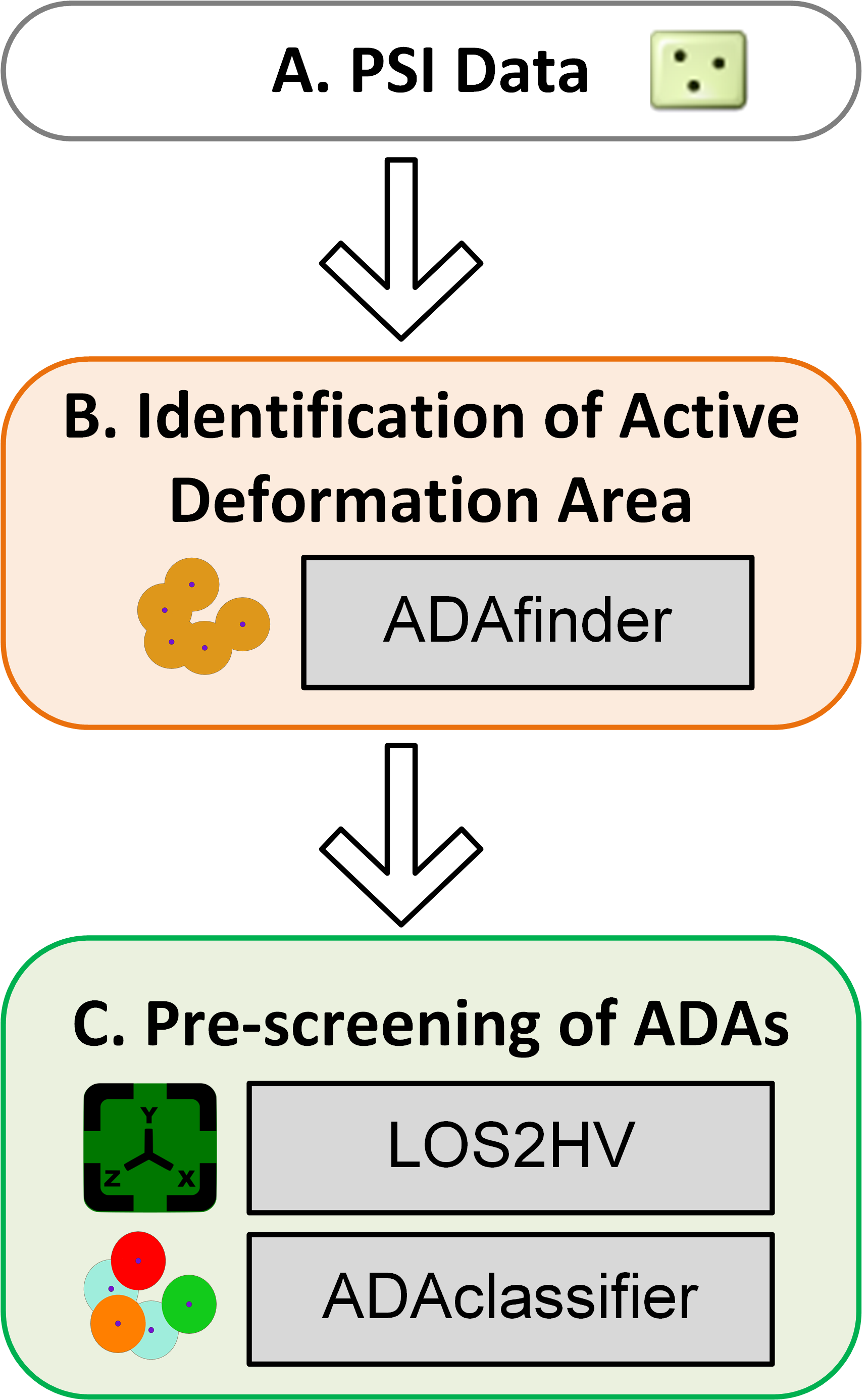
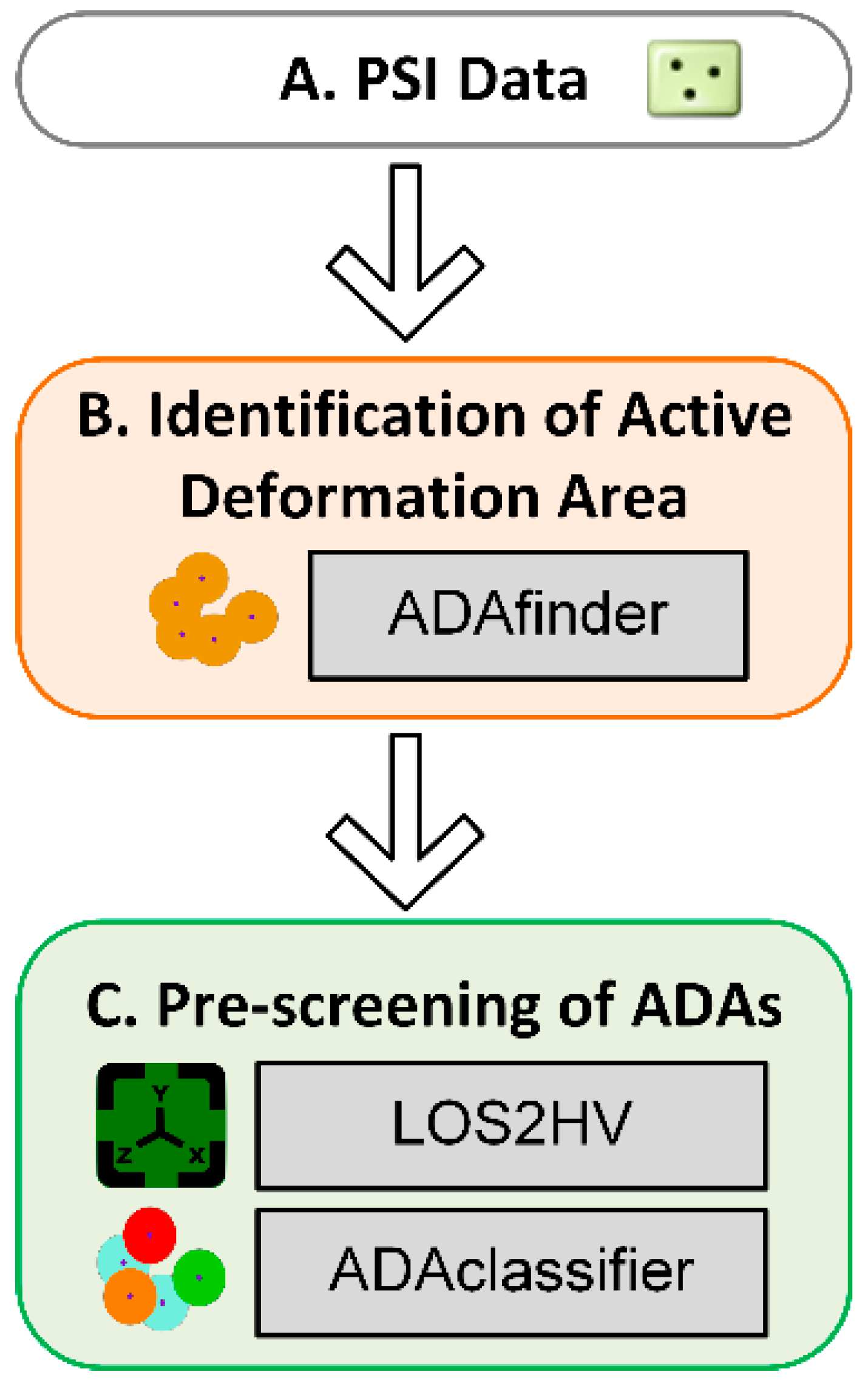
2.1. Chain for The Semiautomatic Classification of Active Deformation Areas

In this section, the procedure proposed to identify and classify ADA is presented. Additionally, the tools that implement the methodology and the required ancillary data are also described. The general scheme of the procedure is shown in Figure 1, consisting of two modules:
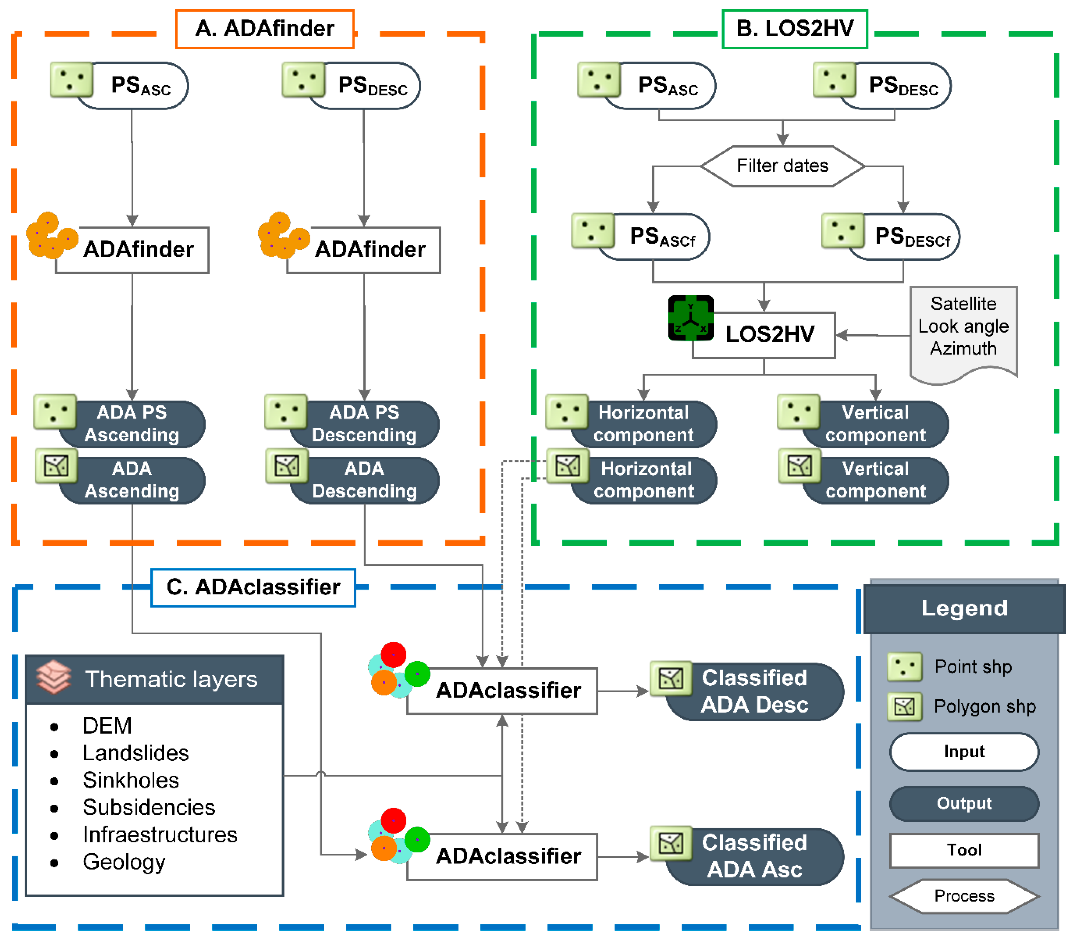
  • Identification of ADA—in this module the PSI data are analyzed to extract the ADA according to the methodology proposed by Barra et al. [17]. To this aim, the app ADAfinder has been implemented. The derived product consists of a map of ADA that contains the areas showing active deformation represented as polygons. This is an intermediate product for the next step.
  • Pre-screening of ADA—this block performs a preliminary classification of the ADA previously identified using auxiliary information. This process is carried out by means of the applications LOS2HV and ADAclassifier. The output of this step consists of a set of maps containing information about the potential geohazards underlying each ADA.
It should be pointed out that the applications ADAfinder, LOS2HV and ADAclassifier have been developed in C++ for efficiency reasons, and both a command line and a Graphical User Interface (GUI) versions of such tools are offered to the user. The GUI simplifies noticeably the operational procedure; the command line version may be used to integrate this tool into a batch production line, if necessary. It is worth mentioning that these apps are available on request.
A more detailed description of the software of applications ADAfinder and ADAclassifier can be consulted in [24,25], but a summary is included in next subsections for the sake of completeness. Finally, within this section, the proposed operational scheme is comprehensively defined.

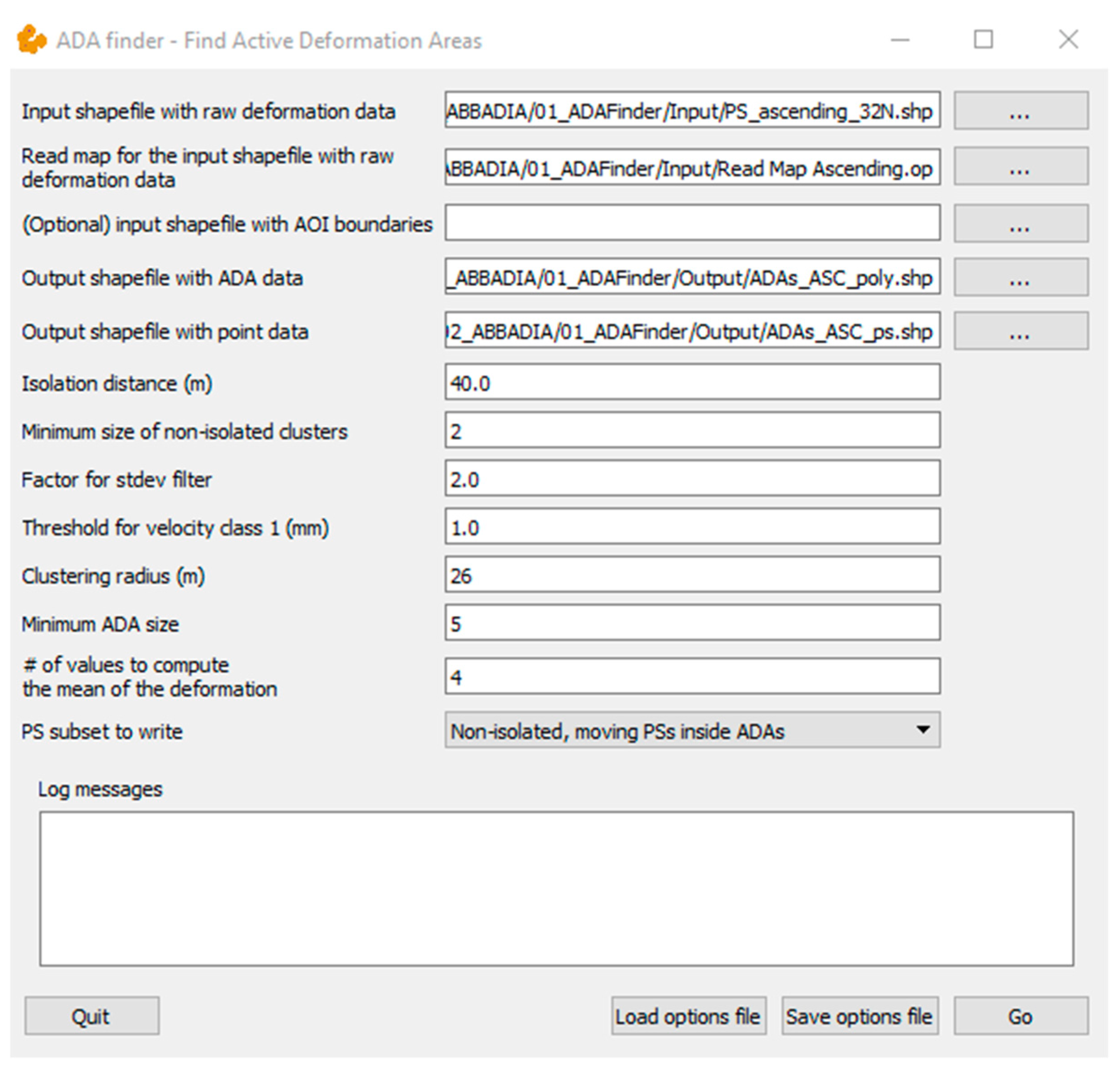
2.1.1. Identification of Active Deformation Areas (ADAfinder)

The role of ADAfinder, the first tool in the toolset, is twofold: to identify the areas where deformation processes—no matter their kind—are taking place, and provide the level of reliability of each identified ADA, based on a noise evaluation of the PS deformation data within each ADA. The tool requires a single ESRI shapefile as input, which must contain the PSs to be processed, including both the (projected) coordinates and deformation time series for each PS for allowing ADAfinder to work properly.
The user has to define seven parameters (Figure 2):
  • The isolation distance that defines the radius of isolation around a PS. This parameter is set to perform a PS filtering aimed at reducing the general noise of the PS deformation map. PSs with no neighbors within such radius are considered isolated and thus removed. It is recommended to adopt twice the resolution of the SAR images dataset for this parameter. Therefore, a distance of 40 m has been adopted in our test sites. This isolation distance is also used to detect outlier PS.
  • The minimum number of active PS within the isolation distance. When within the isolation distance there are fewer active points than the number specified (“Minimum size of non-isolated clusters”), the PS being checked is considered outlier and removed. This condition is applied to clean sparse measurements and points with strong discrepancy with respect their neighbors, i.e., isolated active PS (outliers).
  • The multiplication factor of the standard deviation (σ) of velocities. The definition of the velocity threshold to consider a PS as active or non-active is based on the standard deviation (σ) of the PS velocities of the deformation map that includes all PS [5]. σ can be considered as an indicator of the general sensitivity of the map to measure movements, since it provides information about its noise level [17]. Depending on the case, the user can choose a different multiplication factor to be applied to σ for the velocity threshold definition. Commonly, values comprised between 1⋅σ and 2⋅σ are adopted as stability threshold. In the test sites shown in this work, a value of 1.5⋅σ has been adopted.
  • Velocity threshold to consider an ADA as belonging to class 1 or 2 has to be defined by the user. In this work, an ADA belongs to class 1 if the absolute value of the maximum velocity is higher than the defined velocity threshold or 2 if the velocity is comprised between 1.5⋅σ and the velocity threshold.
  • The radius of influence to consider the active PSs as belonging to the same cluster (i.e., those PSs which are within the “Clustering radius” are considered as members of an ADA). In the test areas a value of 26 m, i.e., 1.3 times the lower resolution of the used SAR data (20 m for the Interferometric Wide swath mode acquisition of Sentinel-1), has been adopted.
  • The “Minimum ADA size” is the minimum number of active contiguous PS to be an ADA. A minimum number of three non-aligned points is required since they are used to calculate the slope of the ground surface by means of the best-fit plane by ADA classifier. In the three cases analyzed in this work a value of 5 has been adopted.
  • The number of “values to compute the mean of the deformation” states the number of the last n values of each time series that are used to compute the average accumulated deformation. The aim of this average is to minimize the influence of potential noise associated with each single value. This number is usually set to 4 or slightly higher. In this work, a value of 4 has been considered.
The output consists of two ESRI shapefiles. The first one defines the boundaries of the ADA, while the second one contains the PS (a) making the ADA and, (b) optionally, all the other PSs that, although not being part of the detected ADA, have passed all the filters set by the algorithm. One of the attributes defining the output ADA is the quality index (QI) [17], which states the degree of reliability of each detected ADA as a variable taking only four possible values going from “not reliable” (Class 4) in the worst case up to “highly reliable” (Class 1) in the best one. The QI assesses the quality of the deformation measurements within each ADA, evaluating both the noise of each active point time series and the spatial uniformity of the estimated deformations in time.

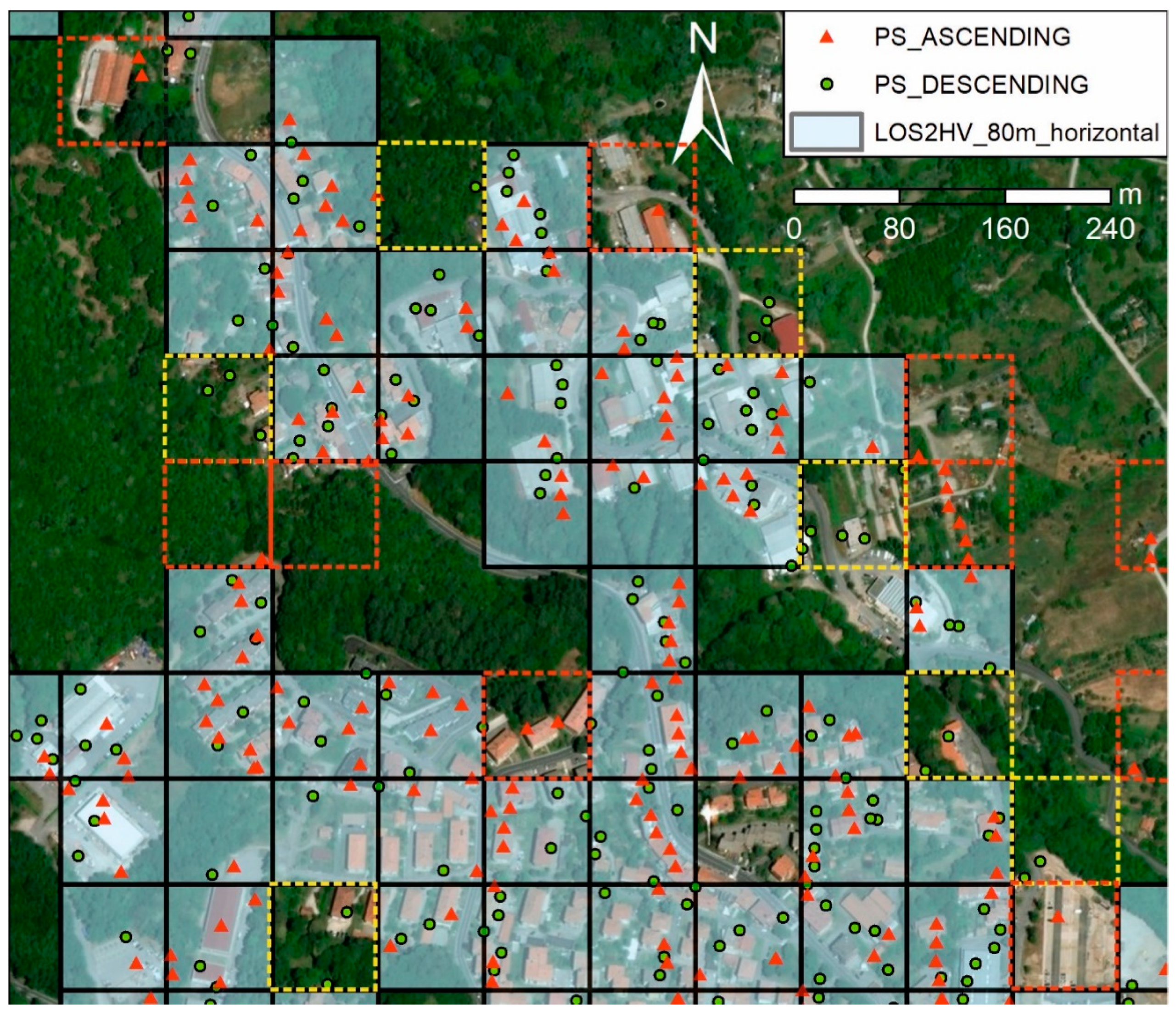
2.1.2. Decomposition of LOS Displacements into Horizontal and Vertical (LOS2HV)

One of the inputs required by the ADAclassifier tool (see Section 2.1.3. below) to classify the ADA extracted by the ADAfinder are the horizontal east-west components of the movement undergone by the PSs. The LOS2HV tool is able to automatically decompose the LOS velocity into horizontal and vertical components. This application takes two datasets as input (ascending and descending) measuring displacements along the LOS, and the geometry of the SAR acquisitions (i.e., look angles and LOS azimuths of both datasets), required to perform the decomposition according to the formulation described in [26]. The outputs are two new files containing the aforementioned horizontal east–west and vertical components of such movement. All the files intervening in this process are ESRI shapefiles. At this point, it must be kept in mind that InSAR geometry only allows the calculation of horizontal displacements along E–W [26,27] and, thus, those ADA presenting N–S displacements will be neither identified nor classified. Unfortunately, this is an inherent drawback of InSAR geometry.
LOS2HV computes the components for the area including the terrain covered by both the ascending and descending datasets. Such an area is thus tessellated (Figure 3)—the size of the grid is decided by the user (Grid spacing)—,and then the horizontal ( V E W ) and vertical ( V V ) components are computed for only those tesserae in which there exist PS from both the ascending (Va) and descending ( V d ) datasets. In the test sites analysed in this paper, a grid size equal to 80 m, which corresponds to four times the PS size, has been used. For each cell, the displacement rates are then averaged, and their horizontal and vertical components are computed according to the following expressions, as described in [26]:
V E W = [ V d c o s ( α d ) V a c o s ( α a ) ] [ c o s ( π / 2 α d ) · c o s ( 3 π / 2 θ d ) c o s ( α d ) c o s ( π / 2 α a ) · c o s ( 3 π / 2 θ a ) c o s ( α a ) ]
V V = [ V d c o s ( π / 2 α d ) · c o s ( 3 π / 2 θ d ) V a c o s ( π / 2 α a ) · c o s ( 3 π / 2 θ a ) ] [ c o s ( α d ) c o s ( π / 2 α d ) · c o s ( 3 π / 2 θ d ) c o s ( α a ) c o s ( π / 2 α a ) · c o s ( 3 π / 2 θ a ) ]
where α d and α a are the descending and ascending incidence angles, respectively, and θd and θa are the azimuth of the LOS in radians for descending and ascending orbits, respectively.

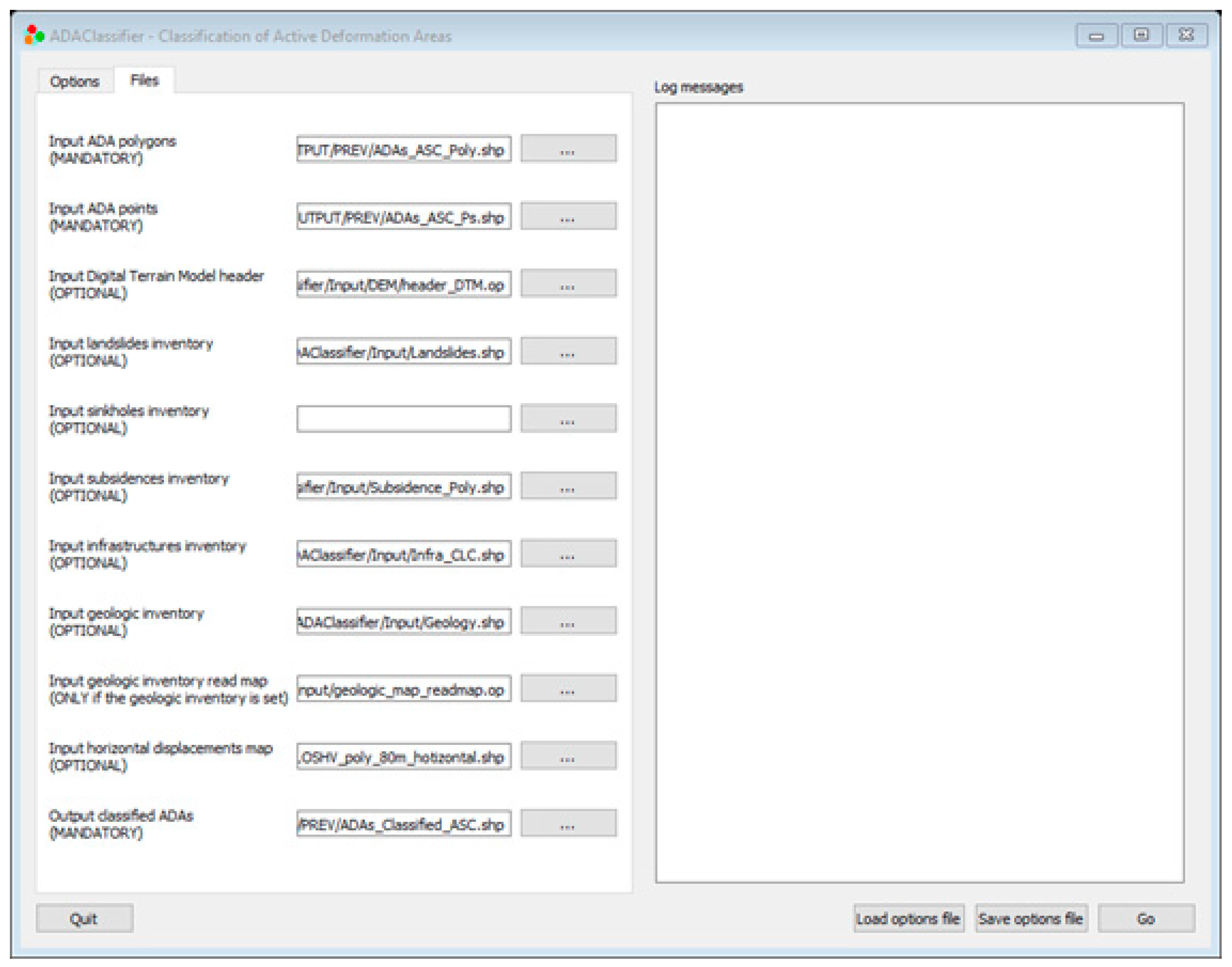
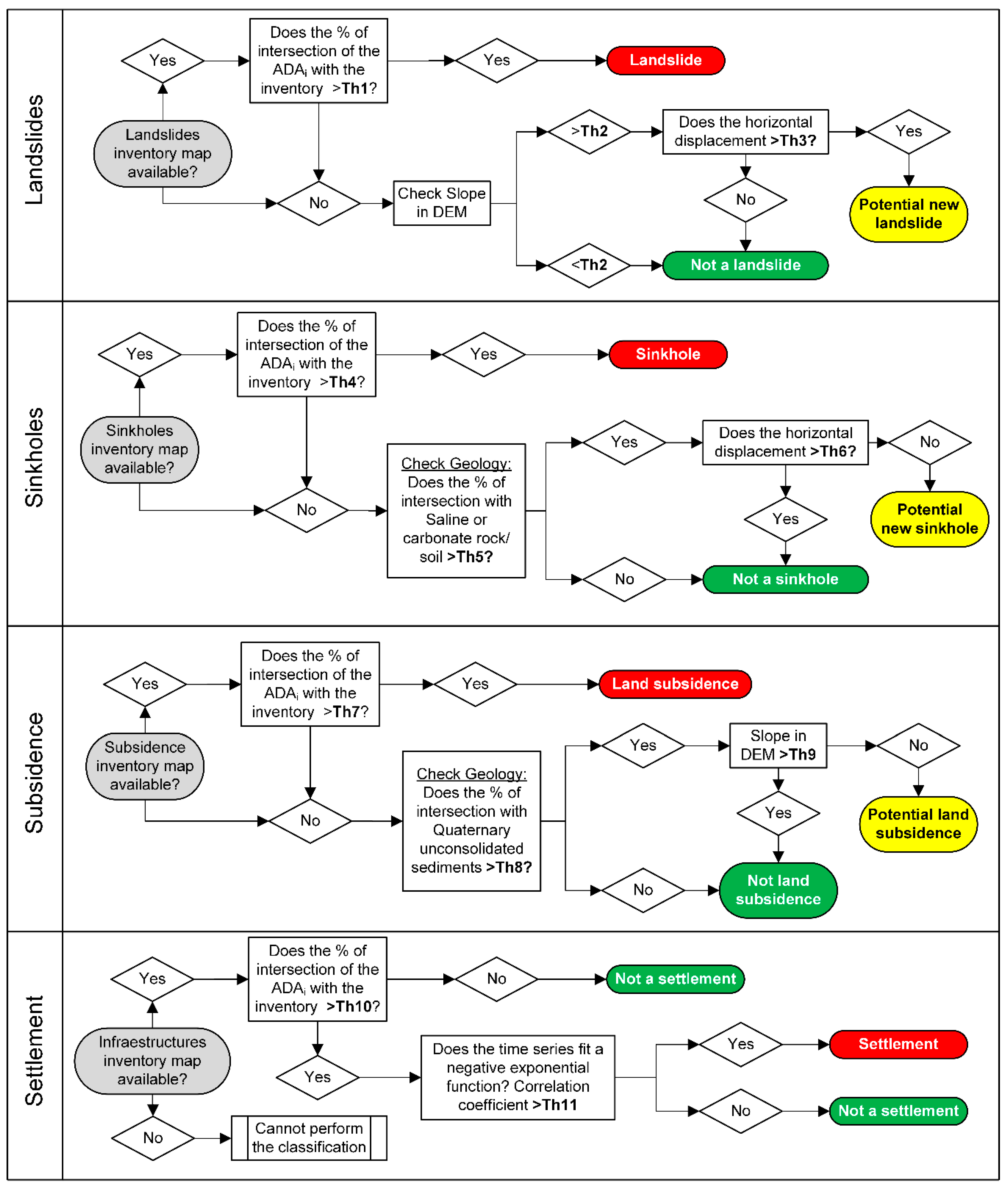
2.1.3. Classification of Active Deformation Areas (ADA Classifier)

ADAclassifier takes the outputs of ADAfinder and LOS2HV plus some ancillary information as the inventory maps of different geological hazards, the DEM, the geological map, and the vector map of the urban areas, to detect up to four different kinds of deformation phenomena, namely landslides, sinkholes, land subsidence areas, and constructive or consolidation settlements (Table 1). Note that many of these ancillary inputs will not exist in many occasions; to make the application more useful, ADAclassifier (Figure 4) performs the classification process according to data availability. ADA polygons and PS points are mandatory, but some inventories are optional. When they are available, these inventories are used to classify the ADA if the intersection between the ADA polygon and an inventory is over the corresponding defined threshold (Th1, Th4, Th7 and Th10 in Figure 5). If the inventories are not available, ADAclassifier continues performing the classification process according to the decision tree shown in Figure 5, identifying the potential risks. A DEM, the horizontal displacements derived from LOS2HV and the available geological maps, are always used in these steps. Consequently, the lack of any of them makes the classification process impossible.
Table 1 depicts the dependencies between the different classification subprocesses and the data needed to perform them or, if the table is read by rows, it describes the classification subprocesses that may, or may not, take place when a file is available or not.
It is worth mentioning that threshold values (Thxi) have to be defined by the user for each decision-making of the classification process. Some thresholds, i.e., Th1, Th4, Th7 and Th10, are related to the spatial overlap of the ADA and the thematic layers containing the inventories of landslides, sinkholes, land subsidence, and infrastructures (i.e., urban areas), if any, respectively. Other spatial thresholds, i.e., Th5 and Th8, check the overlapping of the ADA and the lithological units of the geological map previously classified by the user as potentially soluble (i.e., saline and carbonate rocks) or compressible (i.e., unconsolidated sediments). It should be noted that these thresholds have to be set in accordance to the working scale, the update status of the maps, and the InSAR data resolution to consider potential georeferencing and spatial accuracy errors derived from the delineation of the inventory maps and the InSAR processing. Therefore, when the percentage result of measuring the intersection between the PS set included within the contour of an ADA and the polygons in the inventory is equal to or exceeds the corresponding threshold, it is assumed that the ADA is actually over the mapped feature. A value of 10% has been used in this work according to the characteristics of the used inventory maps.
Th3 and Th6 define the limiting value to consider an ADA as stable or active according to their horizontal displacements. This value strongly depends on the characteristics of the processing, being advisable to adopt a value similar to that considered in ADAfinder, which varies from 1⋅σ to 2⋅σ (an absolute value of 5 mm/year has been considered in this work, that corresponds to extremely slow landslides [28]).
Th2 and Th9 limit the maximum slope in which certain processes can develop or not (i.e., landslides and land subsidence). In the test sites analyzed in this work it was assumed that landslides can develop on slopes higher than 5° [29,30], whereas, on the other hand, land subsidence occurs on flat areas with lower slopes.
The threshold Th11 provides an evaluation of the goodness of fit of a negative exponential function to the ADA average time series for consolidation settlement processes, recommending a minimum value of 0.9.
The output of ADAclassifier is an extended version of the input ESRI shapefile. The attribute table for each shapefile includes four extra fields. Each of these is a variable taking one of four possible values stating the certainty level of the assessment for one of the four deformation processes that may be tested. The possible values are “it is an X”, “it could be an X”, “it is not an X” and “not checked”, where “X” stands for the name of any of the four processes checked, as for instance, “landslide”. The “not checked” value is necessary because of the optionality of most of the input ancillary files, which prevents checking some of the deformation phenomena when one or more of these input files are not available. Additionally, some additional fields are provided by ADAclassifier for each ADA: the percentages of overlapping between the ADA and the different inventory maps, the slope, the mean horizontal velocity and the correlation coefficient of the negative exponential fitted for checking potential consolidation settlements.
Finally, yet importantly, all the detection algorithms are applied to the ADA. This means that, although incongruous, positive results for one or more of the deformation processes are possible; that is, an ADA may be classified, for instance, as a landslide and a sinkhole, simultaneously. Therefore, this methodology has to be considered as a semi-automatic pre-classification or pre-screening process of InSAR data for wide areas and, thus, further expert analysis is required to confirm the deformation process underlying each ADA.

2.1.4. Proposed Operational Scheme
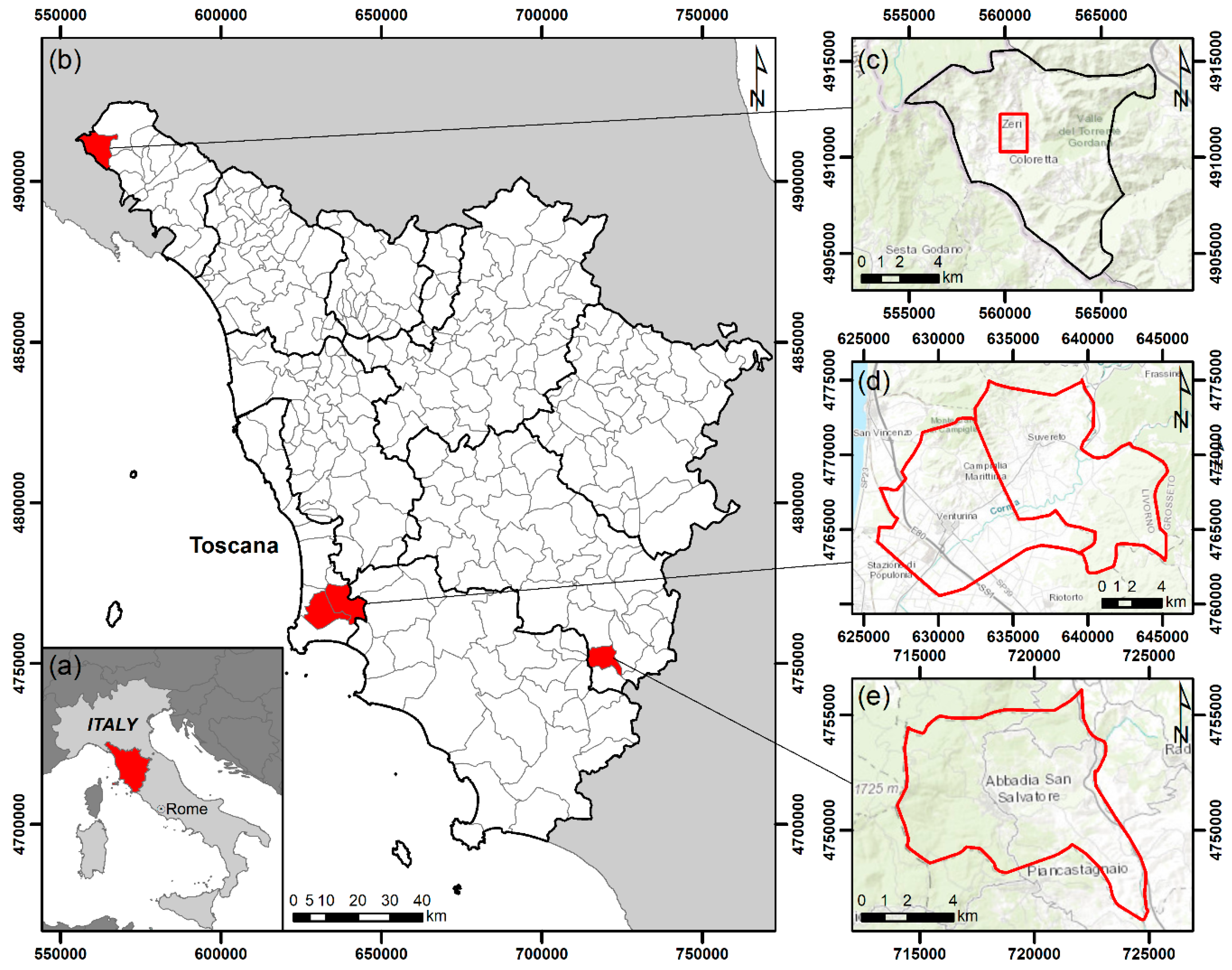
In this subsection the general workflow proposed in this paper to semi-automatically identify and classify ADA, according to the underlying process, from PSI datasets based on the use of the above described tools is detailed (Figure 2). At least one PS dataset (ascending or descending) is required to use this workflow. However, the potential of the method increases when ascending and descending datasets are available since then it is possible decomposing LOS displacements into vertical and horizontal components using the LOS2HV app described in Section 2.1.2. In the following paragraphs the proposed methodology is described in detail:
Step1. Firstly, available ascending and/or descending PS dataset/s of the area of interest is/are uploaded and the input files for each dataset are configured. These files are mandatory for the ADAfinder since they contain information about the structure of the attribute table of the input PS shapefile datasets. Secondly, the different parameters, described in Section 2.1.1., are defined by the user and the app can be executed. This process is performed independently for both the ascending and descending datasets (Figure 6A). The results consist of two shapefiles containing the polygons that define all ADA and the PS included by each of them, jointly with their attributes (e.g., the QI of each ADA).
Step 2. When ascending and descending datasets are available, in parallel to the previous processing block, LOS displacements for each dataset are decomposed into vertical and E-W horizontal directions using the LOS2HV app (Figure 6B) described in Section 2.1.2. To carry out this task, previously, ascending and descending datasets have to be initially filtered in order to ensure the match between the dates of the ascending and descending datasets for the common time period of both time series. Besides, the geometry of the satellite for both acquisitions must be defined. The outputs of this software consist of four shapefiles: two containing the point’s horizontal and vertical components of displacement, and two shapefiles containing the tessellation in which horizontal and vertical components of displacement have been computed.
Step 3. Once the ADA have been identified and horizontal displacements have been computed, the next step consists in the classification of the detected ADA, using the app ADAclassifier (Figure 6C). To this aim, ancillary data described in Section 2.1.3. are required as well as the horizontal displacements derived from LOS2HV. The different thresholds Thxi described above have also to be defined by the user. The outputs consist of two shapefiles containing the classification of the ascending and descending ADA identified in Step 1.

2.2. Test Areas

Over 100,000 landslides are mapped in the Tuscany Region (central Italy), a large part of them are considered as active [31]. Subsidence phenomena are important as well, affecting urban areas along coastal deltas and in agricultural areas where water overexploitation is common [32]. In this paper, three case studies are presented, which are selected from different municipalities affected by landslides or subsidence phenomena (Figure 7). In particular, the municipalities of Zeri (Patigno and Coloretta hamlets) and Abbadia San Salvatore, areas located in the Northern Apennines, are two valuable examples of territories widely affected by active slope processes. On the other hand, the Campiglia Marittima and the nearby Suvereto municipalities have been selected for the presence of widespread subsidence phenomena.
More in detail, Patigno is located along a south-east exposed slope affected by an active complex landslide involving the entire hamlet. The decennial motion of the landslide seriously damaged the road network and a large part of the buildings of the hamlet [33,34]. Coloretta, located a few kilometres southwestern than Patigno, is affected by several landslides with different magnitudes of motion that caused various damage levels on buildings and infrastructures [34]. Campiglia Marittima and Suvereto are placed along the Cornia river valley and are characterized by intensive agriculture thanks to the presence of highly productive aquifers. Thus, land subsidence phenomenon is caused by water withdrawal that triggers long-term consolidation of unconsolidated loamy and silty sediments [35]. The surroundings of the fluvial valley are characterized by widespread slope processes along the gentle valley flanks. Abbadia San Salvatore is located along the eastern flank of the Monte Amiata, an extinct volcanic system. Because of its geological and geomorphological setting, the municipality is affected by several active landslides [36], especially in its most recently urbanized portion. Landslides caused high economic losses in the last 30 years, in one case leading to the evacuation of some private buildings.

2.3. Input Datasets

2.3.1. InSAR Data

The processed InSAR Sentinel-1 data derive from the agreement “Monitoring ground deformation in the Tuscany Region with satellite radar data” concluded with the Regional Government of Tuscany, Italian Civil Protection Department, and the LaMMA (Environmental Modelling and Monitoring Laboratory for Sustainable Development) consortium.
Sentinel-1 is a constellation composed of two twin satellites acquiring images at C-band (central frequency 5.4 GHz and wavelength 5.6 cm) which grants a 6-days revisiting time. Thanks to their geographical position, the three test areas are covered by four different satellite tracks, two in ascending orbit (15 and 117) and two in descending orbit (95 and 168). Table 2 shows the characteristics of the Sentinel-1 images used. The temporal baselines of the selected interferograms for ascending and descending orbits vary from 6 to 1020 days and from 6 to 1032 days, respectively. Additionally, the spatial baselines vary from 13 to 180 m and from 7 to 126 m for ascending and descending orbits, respectively.
The tracks have been processed separately by means of the SqueeSAR algorithm, developed by Ferretti et al. [37]. This interferometric technique relies on the definition of radar stable targets, being coherent Permanent Scatterers (PS) [4] or partially coherent Distributed Scatterers (DS) [37]. The combination between point-wise (PS) and areal (DS) targets allows to increase considerably the number of measurement points in peri-urban areas and to guarantee a higher signal to noise ratio in the derived time series of displacement [37].
Each measurement point is characterized by a velocity value interpolated over the acquisition time period, a value for the displacement at each acquisition date, and some quality parameters such as the standard deviation of the velocity or the statistical coherence of the time series with respect to the linear model. The measures are differential, thus referred to a common reference point assumed motionless and here selected on the basis of geological considerations, geomorphological ancillary data, previous interferometric results, and GNSS (Global Navigation Satellite System) data. The latter are acquired by permanent stations belonging to the European GNSS Permanent Network and to the Italian GNSS Geodetic Reference System (Rete Dinamica Nazionale). For further information about the GNSS network, we refer to Del Soldato et al. [38].
The SqueeSAR algorithm can achieve a 2·σ accuracy of 5 mm on the single displacement measures with a geocoding error lower than a few meters. Thanks to the large number of images acquired over a three years-time period (more than 100) it is possible to reach a precision of the velocity estimation close to 1 mm/year [21].
The original processing covers the entire Tuscany Region and performs a continuous monitoring update of ground deformations as described in Raspini et al. [21]. In this work we focused on three subareas whose general ascending and descending LOS velocity maps are presented as supplementary material (Figures S1–S3).

2.3.2. Ancillary Data

A DEM with a 10 m cell resolution of the Tuscany Region was used for deriving the elevation of the PS contained in each ADA. The mean slope of each ADA was then automatically calculated by ADAclassifier fitting a plane to these points for classification purposes. Furthermore, the updated Italian Landslide Inventory map—IFFI project—of the region of Tuscany [31] and the subsidence contour map [32] of the Tuscany region were used. The landslide inventory map of the entire Tuscany region provides a detailed picture of the distribution of landslides in 2007, and it is composed by more than 100,000 landslides that are classified into typologies and according to their state of activity: active, dormant, stabilized, and undetermined. It was produced using conventional, e.g., geomorphological field mapping or stereoscopic aerial photograph interpretation, and innovative techniques, e.g., analysis of high-resolution DEM or InSAR data interpretation and analysis. The subsidence areas were highlighted by the analysis and interpretation of PSI products derived from different satellites (ERS 1/2, ENVISAT and Sentitnel-1) and considering only the contour of vertical velocity (in mm/year) after the decomposition of the LOS velocity [32].
A geological map is available for consulting and downloading on the Tuscany Region website at 1:10,000 nominal scale. In the three test areas, the geological map was reclassified by experts in order to state those geological units from which we can expect that land subsidence or sinkhole processes develop. In this sense, dissolution processes in carbonate rocks were potentially associated with Jurassic limestones in Abbadia San Salvatore, with Jurassic limestones and Pleistocene travertines in Campiglia Marittima–Suvereto and with Eocene limestones in Zeri. Saline rocks were not found in the study areas. Finally, land subsidence potential was attributed to all Holocene detritic alluvial deposits existing in Campiglia Marittima and Suvereto as well as in Zeri.
The CORINE (Coordination of Information on the Environment) Land Cover is available. It was updated in 2013 by the Tuscany Region website, by the Web Map Service (WMS), for downloading [39]. It is more precise than the CORINE Land Cover (CLC) of the entire Italian territory which was updated in 2012. It provides a division into five classes at the first level, and they are hierarchically subdivided into three levels which are gradually more precise. The CLC second level classes referred to the urban fabric and to industrial, commercial and transport unit areas were selected to perform the classification of the consolidation processes.

3. Results

The methodology proposed in this work (Section 2.1.4) has been employed for the semi-automatic identification and pre-screening of deformational processes, and it was applied in the three case studies described in Section 2.2. using Sentinel-1 datasets and ancillary data (Section 2.3). The results are presented in this section.

3.1. Active Deformation Areas

As described in previous sections, the first step of the proposed methodology consists of the identification of ADA using the app ADAfinder. Table 3 summarizes the results of the ADA recognized in the three test sites (Figure 5, Figure 6 and Figure 7).
In Abbadia San Salvatore 10 ADA, 6 from ascending and 4 from descending datasets, covering a total surface of 0.095 and 0.034 km2, respectively, have been recognized. The size of the ADA varies from 0.008 to 0.031 and 0.008 to 0.009 km2 and from 6 to 20 and 6 to 9 PS for ascending and descending datasets, respectively.
Campiglia Marittima and Suvereto test site shows 8 ADA (4 derived from ascending and 4 from descending tracks) occupying a surface of 0.034 and 0.037 km2 for ascending and descending datasets. The size of the ADA found varies from 0.006 to 0.015 and 0.005 to 0.024 km2 and from 5 to 15 and 5 to 14 PS in ascending and descending datasets, respectively.
Finally, 10 ADA (5 from ascending and 5 from descending tracks) are also identified in the test site of Zeri covering a total surface of 0.369 km2 (0.238 and 0.131 km2 for ascending and descending orbits, respectively). The size of the ADA found in this test site varies from 0.006 to 0.074 and 0.006 to 0.082 km2 and from 5 to 62 and 5 to 54 PS for ascending and descending tracks, respectively.

3.2. Horizontal and Vertical Displacements

The east-west and vertical components of displacement of the three test sites have been calculated using an 80 m grid size by means of the LOS2HV app (Figures S4, S8 and S12). For this calculation, all PS available in the test sites (total number of PS in Table 4), mainly concentrated over the urban areas (Figure 8, Figure 9 and Figure 10), have been considered as potential candidates. Subsequently, the decomposition of the velocity has been performed only in those cells in which ascending and descending PS are available: 327, 1594 and 73 cells for the grids for Abbadia San Salvatore, Campiglia Marittima and Suvereto, Zeri, respectively.
It is worth noting that for the three test areas some PS have not been used to calculate the east-west and vertical components because the inexistence of coincident PS from both datasets (i.e., ascending and descending) within the same cell. The number of PS effectively used to decompose the LOS velocity is equal to 371 (16.4%), 3210 (28.0%) and 102 (17.6%) for Abbadia San Salvatore, Campiglia Marittima–Suvereto and Zeri, respectively. It means that a considerable volume of information is lost during the conversion of LOS velocity into vertical and horizontal velocities. The horizontal displacements derived from LOS2HV are shown in Figures S4, S8 and S12 from Supplementary material and are used for the subsequent classification of landslides and sinkholes by ADAclassifier.

3.3. Classified Active Deformation Areas

The ADA derived from the analyzed InSAR datasets (Section 3.1.) have been automatically classified according to the methodology described in 2.1.4 considering the horizontal displacements (Section 3.2.) and the available ancillary data (i.e., geological, landslides, subsidence and land use maps). The results of the three test sites and the time series of some characteristic PS from ascending and descending orbits are shown in Figure 8, Figure 9 and Figure 10. For the screening of each study area, the four potential deformational processes are evaluated for every ADA. As a result, for each ADA the different considered geological–geotechnical processes can be confirmed, considered as potential or rejected by the software. Additionally, when the compulsory ancillary information for the pre-screening process is not available the ADA is not classified. It is worth noting that, for a clearer presentation of the results, only the classification of the geological–geotechnical deformational processes that predominates in each area are presented in Figure 8, Figure 9 and Figure 10.
In Abbadia San Salvatore the ten existing ADA found (6 from ascending and 4 from descending datasets) have been classified as landslides (Figure 8 and Table 3) since they match the available inventory of landslides in percentage higher than 10% (i.e., the threshold Th1 in Figure 5 is equal to 10%). The maps depicting the classification of the ADA into land subsidence, consolidation settlements and sinkholes are shown in Figures S5–S7 from Supplementary materials).
In Campiglia Marittima–Suvereto, eight ADA (four from ascending and four from descending datasets) were found and classified according to the proposed algorithm (Figure 9 and Table 3). In detail, the pre-screening performed using ADAclassifier indicates that six ADA (three from ascending and three for descending datasets) correspond to land subsidence because they match the available land subsidence map [32]. One additional ADA is classified as potential land subsidence since, although it is not contained within the land subsidence area, the existence of alluvial detritic sediments from the Quaternary (Holocene and Pleistocene) and a flat relief (with slopes lower than 5°) suggests that the detected displacements are related with land subsidence processes and a landslide phenomenon can be safely excluded. Finally, one ADA has not been classified as land subsidence since it does not match neither the land subsidence area nor the geological units of unconsolidated sediments. This ADA does not satisfy any of the conditions stated for landslides, sinkholes, and settlements either, and thus it is labeled as “not classified”. The maps depicting the classification of the ADA into landslides, consolidation settlements and sinkholes are shown in Figures S9–S11 from Supplementary materials).
In Zeri, the five existing ADA found for the ascending dataset have been classified as landslides since they match the available landslides inventory of the area in a percentage higher than 10% (Figure 10 and Table 3). For the descending dataset only four ADA are pre-screened as landslide (Figure 10 and Table 3). The remaining ADA, located in the urban area of Coloretta (Zeri) is not classified into any specific type of deformational process since it does not match neither the available inventory of landslides nor the parameters for consolidation processes. The maps presenting the classification of the ADA into land subsidence, consolidation settlements and sinkholes are shown in Figures S13–S15 from Supplementary materials).

4. Discussion

In this paper, a procedure has been proposed for the identification and pre-screening of Active Deformation Areas using InSAR datasets, and it has been tested in three areas in Italy using Sentinel-1 constellation datasets.
The main advantage of this method is the possibility of semi-automatically generating thematic maps of ADA and their potential underlying deformation processes for wide areas based on InSAR datasets. This information is of particular interest for providing support for the management and the administration of the territory and the infrastructures.
Another remarkable feature of the methodology is its high processing capacity. The performance of the apps developed for the implementation of the methodology meets the expectations. The equipment used for processing the three test sites was an Intel Core i7-2670QM at 2.2 GHz, 4 cores, 8 threads, 6 MB cache, 8 GB RAM, 250 GB SSD disk and Windows 10, 64 bits. Table 4 shows the characteristics of processed datasets and inventories for each step of the proposed methodology, as well as the outputs of the ADAclassifier. The performance testing of the software showed that the computer needed around 1 s to identify the ADA (step 1) from up to 11,472 PS (Table 4). Similarly, less than 1 s is required to decompose LOS displacements into vertical and horizontal ones (step 2) in up to 1594 cells using 8262 PS (Table 4). Finally, the same time is spent to classify the ADA checking the six available classification processes (step 3) (Table 4). The manual process for the development of these three stages may require from around 15 minutes to some hours. This means that the designed processing chain is more than 300 times faster and eliminates the chance of human errors and requires only a post-processing expert check.
The methodology suffers the same inherent limitations of InSAR, i.e., the lack of coherence over some areas, the limitations of the acquisition geometry, and the measurable displacement range, since InSAR datasets constitute the main input. Although the use of other SAR sensors and geometries can partially overcome this drawback, this limitation is sometimes inevitable and could provide a biased picture of the reality of the areas in which this methodology is applied, hiding important deformations about which satellites are “blind”. In this sense, it must be emphasized that due to the nearly north–south orbit direction of SAR satellites, InSAR is only sensitive to the up–down and east–west directions displacements [27], but not to north-south ones. This fact also could lead to the wrong pre-screening of ADA in which horizontal displacement rates derived from LOS2HV are considered (i.e., landslides and sinkholes according to the decision tree shown in Figure 5).
Another important drawback is the dependence on ancillary information for the classification of the ADA. This information is sometimes unavailable, incomplete, or not updated, hindering the pre-screening tasks. In fact, as shown in Table 1, although some ancillary information is optional (i.e., landslide, sinkhole, land subsidence, and infrastructures inventory maps) most of the ancillary data have to be provided to the software for the implementation of the methodology. In this sense, some tests have been performed to evaluate the robustness of the classification process. To this aim, the test areas of Campiglia Marittima–Suvereto and Zeri have been classified using ADAclassifier both considering the optional data and without considering them (i.e., the inventory of landslides, land subsidence and infrastructures; Figure 11).
In the test site of Campiglia Marittima and Suvereto all ADA classified as land subsidence when considering the land subsidence inventory map were classified as potential land subsidence when the auxiliary information was not used (Figure 11a). In Zeri, six ADA of ten were duly classified (five as landslides and one as an unknown process). Three ADA not classified as landslides in spite of being mapped as landslides in the inventory map where placed in the urban areas of Coloretta and Patigno hamlets (Zeri), exhibiting a smooth ground surface with slopes lower than the threshold (Th2) of 5° (i.e., between 3.1 and 4.8°). The remaining ADA presented a slope of 7.2° and was not classified as landslide since its horizontal velocity was 3 mm/year, i.e., lower than the threshold Th3 defined as 5 mm/year. Therefore, the false negatives when classifying these ADA can be considered as rare cases since below 5° there is a very low landslide probability [29,30]. Despite some misinterpretations on the pre-screening process, these results confirm the robustness of the procedure defined for the preliminary classification of the ADA.
Consolidation processes and sinkholes were not detected in the test areas since the conditions defined in Figure 5 were not satisfied. For consolidation processes, the time series of the ADA placed over urban areas did not fit negative exponential functions properly as illustrated in Figure 8b, Figure 9b and Figure 10 b, and thus these processes are rejected. It should be noted that sinkholes and consolidation potential of the geological units from the geological map have been stated by focusing solely on the description of the lithologies included in the geological map, as explained in Section 2.3.2. Obviously, this potential can be discarded, or new geological units can be added when more comprehensive and detailed geological and geotechnical information is available.

5. Conclusions

This paper presents a new and simple methodology aimed to semi-automatically identify clusters of active PS and preliminarily relate them to different potential types of geological–geotechnical deformational processes. This approach consists of three main steps aimed to: (i) identify active deformation areas using PSI datasets, (ii) decompose ascending and descending LOS PSI data into vertical and horizontal components, and (iii) pre-screen the ADA into different deformational geological–geotechnical processes. Three specific apps have been programmed in C++ language to automatize and optimize the processing chain. The outputs present a high compatibility with GIS environments for analysis and representation purposes.
The performed analyses show that the methodology is quite robust and provide satisfactory results for preliminary analysis of active deformational processes over wide areas.
As a final comment, it is worth noting that the proposed methodology is especially suitable for not InSAR-expert final users and wide areas, allowing to quickly and semi-automatically identify and pre-screen active deformation areas to identify the potential geological–geotechnical deformational processes underlying the detected displacements. Then, this methodology should be considered as a preliminary classification procedure for regional scale analyses. However, for further detailed and in-depth studies, the classification of each ADA should be confirmed trough expert opinion of geoscientists or geological engineers and/or in situ data. Furthermore, it is also very important to keep in mind the inherent limitations of InSAR technique associated with the lack of coherence, the acquisition geometry and the measurable displacement range, that could lead to an under-identification of active processes affecting the areas under study.

Supplementary Materials

The following are available online at https://0-www-mdpi-com.brum.beds.ac.uk/2072-4292/11/14/1675/s1: Figures S1–S3. General map of InSAR LOS displacements of the three test cases. Figures S4–S7. Map of E-W displacements and classification of ADA as land subsidence, consolidation settlements and sinkholes, respectively, of Abbadia San Salvatore. Figures S8–S11. Map of E-W displacements and classification of ADA as landslides, consolidation settlements and sinkholes, respectively, of Campiglia Marittima and Suvereto. Figures S12–S15. Map of E-W displacements and classification of ADA as land subsidence, consolidation settlements and sinkholes, respectively, of Zeri.

Author Contributions

Conceptualization R.T. and J.A.N.; methodology, R.T., A.B., O.M., M.C. (Miguel Cano), J.L.P., A.R. (Adrián Riquelme), G.H. and J.M.L.-S.; software, J.A.N., M.C.-G., M.C. (Michele Crosetto) and A.B.; validation and formal analysis R.T., J.I.P., J.A.N., M.C.-G., M.C. (Michele Crosetto), M.C. (Miguel Cano), J.L.P., A.R. (Adrián Riquelme), M.D.S., L.S., N.C., J.L.-S., A.R. (Alfredo Ramón), S.B., F.R., S.I., M.C. (Mario Costantini) and F.T.; resources, M.D.S., L.S., S.B., F.R., F.N., A.F. and N.C.; writing—original draft preparation, R.T.; writing—review and editing, all.

Funding

This research was funded by the Shift2Rail Joint Undertaking under the European Union’s Horizon 2020 research and innovation program, with grant agreement No 777630, project MOMIT, “Multiscale Observation and Monitoring of railway Infrastructure Threats” and the Spanish Ministry of Economy, Industry and Competitiveness (MINECO), the State Agency of Research (AEI), and the European Funds for Regional Development (FEDER) under project TEC2017-85244-C2-1-P.

Acknowledgments

The authors want to thank the Tuscany Region for providing the ancillary data needed to perform the analyses.

Conflicts of Interest

The authors declare no conflict of interest.

References

  1. Pepe, A.; Calò, F. A Review of Interferometric Synthetic Aperture RADAR (InSAR) Multi-Track Approaches for the Retrieval of Earth’s Surface Displacements. Appl. Sci. 2017, 7, 1264. [Google Scholar] [CrossRef]
  2. Shanker, P.; Casu, F.; Zebker, H.A.; Lanari, R. Comparison of Persistent Scatterers and Small Baseline Time-Series InSAR Results: A Case Study of the San Francisco Bay Area. IEEE Geosci. Remote Sens. Lett. 2011, 8, 592–596. [Google Scholar] [CrossRef]
  3. Crosetto, M.; Monserrat, O.; Cuevas-González, M.; Devanthéry, N.; Crippa, B. Persistent Scatterer Interferometry: A review. ISPRS J. Photogramm. Remote Sens. 2016, 115, 78–89. [Google Scholar] [CrossRef] [Green Version]
  4. Ferretti, A.; Prati, C.; Rocca, F. Permanent scatterers in SAR interferometry. IEEE Trans. Geosci. Remote Sens. 2001, 39, 8–20. [Google Scholar] [CrossRef]
  5. Ferretti, A.; Prati, C.; Rocca, F. Nonlinear subsidence rate estimation using permanent scatterers in differential SAR interferometry. IEEE Trans. Geosci. Remote Sens. 2000, 38, 2202–2212. [Google Scholar] [CrossRef] [Green Version]
  6. Berardino, P.; Fornaro, G.; Lanari, R.; Sansosti, E. A new algorithm for surface deformation monitoring based on small baseline differential SAR interferograms. IEEE Trans. Geosci. Remote Sens. 2002, 40, 2375–2383. [Google Scholar] [CrossRef] [Green Version]
  7. Casu, F.; Manzo, M.; Lanari, R. A quantitative assessment of the SBAS algorithm performance for surface deformation retrieval from DInSAR data. Remote Sens. Environ. 2006, 102, 195–210. [Google Scholar] [CrossRef]
  8. Lanari, R.; Casu, F.; Manzo, M.; Zeni, G.; Berardino, P.; Manunta, M.; Pepe, A. An Overview of the Small BAseline Subset Algorithm: A DInSAR Technique for Surface Deformation Analysis. In Deformation and Gravity Change: Indicators of Isostasy, Tectonics, Volcanism, and Climate Change; Wolf, D., Fernández, J., Eds.; Birkhäuser: Basel, Switzerland, 2007; pp. 637–661. [Google Scholar] [CrossRef]
  9. Tomás, R.; Li, Z. Earth Observations for Geohazards: Present and Future Challenges. Remote Sens. 2017, 9, 194. [Google Scholar] [CrossRef]
  10. Bianchini, S.; Raspini, F.; Solari, L.; Del Soldato, M.; Ciampalini, A.; Rosi, A.; Casagli, N. From Picture to Movie: Twenty Years of Ground Deformation Recording Over Tuscany Region (Italy) with Satellite InSAR. Front. Earth Sci. 2018, 6, 177. [Google Scholar] [CrossRef]
  11. Samsonov, S.V.; d’Oreye, N.; González, P.J.; Tiampo, K.F.; Ertolahti, L.; Clague, J.J. Rapidly accelerating subsidence in the Greater Vancouver region from two decades of ERS-ENVISAT-RADARSAT-2 DInSAR measurements. Remote Sens. Environ. 2014, 143, 180–191. [Google Scholar] [CrossRef] [Green Version]
  12. Herrera, G.; Gutiérrez, F.; García-Davalillo, J.C.; Guerrero, J.; Notti, D.; Galve, J.P.; Fernández-Merodo, J.A.; Cooksley, G. Multi-sensor advanced DInSAR monitoring of very slow landslides: The Tena Valley case study (Central Spanish Pyrenees). Remote Sens. Environ. 2013, 128, 31–43. [Google Scholar] [CrossRef]
  13. Cignetti, M.; Manconi, A.; Manunta, M.; Giordan, D.; De Luca, C.; Allasia, P.; Ardizzone, F. Taking Advantage of the ESA G-POD Service to Study Ground Deformation Processes in High Mountain Areas: A Valle d’Aosta Case Study, Northern Italy. Remote Sens. 2016, 8, 852. [Google Scholar] [CrossRef]
  14. Raucoules, D.; Colesanti, C.; Carnec, C. Use of SAR interferometry for detecting and assessing ground subsidence. C. R. Geosci. 2007, 339, 289–302. [Google Scholar] [CrossRef]
  15. Costantini, M.; Ferretti, A.; Minati, F.; Falco, S.; Trillo, F.; Colombo, D.; Novali, F.; Malvarosa, F.; Mammone, C.; Vecchioli, F.; et al. Analysis of surface deformations over the whole Italian territory by interferometric processing of ERS, Envisat and COSMO-SkyMed radar data. Remote Sens. Environ. 2017, 202, 250–275. [Google Scholar] [CrossRef]
  16. Tomás, R.; Romero, R.; Mulas, J.; Marturià, J.J.; Mallorquí, J.J.; Lopez-Sanchez, J.M.; Herrera, G.; Gutiérrez, F.; González, P.J.; Fernández, J.; et al. Radar interferometry techniques for the study of ground subsidence phenomena: A review of practical issues through cases in Spain. Environ. Earth Sci. 2014, 71, 163–181. [Google Scholar] [CrossRef]
  17. Barra, A.; Solari, L.; Béjar-Pizarro, M.; Monserrat, O.; Bianchini, S.; Herrera, G.; Crosetto, M.; Sarro, R.; González-Alonso, E.; Mateos, R.; et al. A Methodology to Detect and Update Active Deformation Areas Based on Sentinel-1 SAR Images. Remote Sens. 2017, 9, 1002. [Google Scholar] [CrossRef]
  18. Meisina, C.; Zucca, F.; Notti, D.; Colombo, A.; Cucchi, A.; Savio, G.; Giannico, C.; Bianchi, M. Geological Interpretation of PSInSAR Data at Regional Scale. Sensors 2008, 8, 7469–7492. [Google Scholar] [CrossRef] [PubMed] [Green Version]
  19. Bianchini, S.; Cigna, F.; Righini, G.; Proietti, C.; Casagli, N. Landslide HotSpot Mapping by means of Persistent Scatterer Interferometry. Environ. Earth Sci. 2012, 67, 1155–1172. [Google Scholar] [CrossRef]
  20. Zhao, C.; Lu, Z.; Zhang, Q.; de la Fuente, J. Large-area landslide detection and monitoring with ALOS/PALSAR imagery data over Northern California and Southern Oregon, USA. Remote Sens. Environ. 2012, 124, 348–359. [Google Scholar] [CrossRef]
  21. Raspini, F.; Bianchini, S.; Ciampalini, A.; Del Soldato, M.; Solari, L.; Novali, F.; Del Conte, S.; Rucci, A.; Ferretti, A.; Casagli, N. Continuous, semi-automatic monitoring of ground deformation using Sentinel-1 satellites. Sci. Rep. 2018, 8, 7253. [Google Scholar] [CrossRef]
  22. Solari, L.; Barra, A.; Herrera, G.; Bianchini, S.; Monserrat, O.; Béjar-Pizarro, M.; Crosetto, M.; Sarro, R.; Moretti, S. Fast detection of ground motions on vulnerable elements using Sentinel-1 InSAR data. Geomat. Nat. Hazards Risk 2018, 9, 152–174. [Google Scholar] [CrossRef]
  23. Calò, F.; Ardizzone, F.; Castaldo, R.; Lollino, P.; Tizzani, P.; Guzzetti, F.; Lanari, R.; Angeli, M.-G.; Pontoni, F.; Manunta, M. Enhanced landslide investigations through advanced DInSAR techniques: The Ivancich case study, Assisi, Italy. Remote Sens. Environ. 2014, 142, 69–82. [Google Scholar] [CrossRef] [Green Version]
  24. Navarro, J.A.; Cuevas, M.; Tomás, R.; Barra, A.; Crosetto, M. A toolset to detect and classify Active Deformation Areas using interferometric SAR data. In Proceedings of the 5th International Conference on Geographical Information Systems Theory, Applications and Management, Heraklion, Crete, Greece, 3–5 May 2019; pp. 167–174. [Google Scholar]
  25. Navarro, J.A.; Cuevas, M.; Barra, A.; Crosetto, M. Detection of Active Deformation Areas based on Sentinel-1 imagery: An efficient, fast and flexible implementation. In Proceedings of the 18th International Scientific and Technical Conference, Crete, Greece, 24–27 September 2018. [Google Scholar]
  26. Notti, D.; Herrera, G.; Bianchini, S.; Meisina, C.; García-Davalillo, J.C.; Zucca, F. A methodology for improving landslide PSI data analysis. Int. J. Remote Sens. 2014, 35, 2186–2214. [Google Scholar] [CrossRef]
  27. He, L.; Wu, L.; Liu, S.; Wang, Z.; Su, C.; Liu, S.-N. Mapping Two-Dimensional Deformation Field Time-Series of Large Slope by Coupling DInSAR-SBAS with MAI-SBAS. Remote Sens. 2015, 7, 12440–12458. [Google Scholar] [CrossRef] [Green Version]
  28. Cruden, D.M.; Varnes, D.J. Landslide types and processes. In Landslides: Investigation and Mitigation; National Research Council, Transportation and Research Board Special Report; Turner, A.K., Schuster, R.L., Eds.; Academy Press: Washington, DC, USA, 1996; pp. 36–75. [Google Scholar]
  29. Lee, S.; Ryu, J.-H.; Won, J.-S.; Park, H.-J. Determination and application of the weights for landslide susceptibility mapping using an artificial neural network. Eng. Geol. 2004, 71, 289–302. [Google Scholar] [CrossRef]
  30. Ayalew, L.; Yamagishi, H. The application of GIS-based logistic regression for landslide susceptibility mapping in the Kakuda-Yahiko Mountains, Central Japan. Geomorphology 2005, 65, 15–31. [Google Scholar] [CrossRef]
  31. Rosi, A.; Tofani, V.; Tanteri, L.; Tacconi Stefanelli, C.; Agostini, A.; Catani, F.; Casagli, N. The new landslide inventory of Tuscany (Italy) updated with PS-InSAR: Geomorphological features and landslide distribution. Landslides 2018, 15, 5–19. [Google Scholar] [CrossRef]
  32. Rosi, A.; Tofani, V.; Agostini, A.; Tanteri, L.; Tacconi Stefanelli, C.; Catani, F.; Casagli, N. Subsidence mapping at regional scale using persistent scatters interferometry (PSI): The case of Tuscany region (Italy). Int. J. Appl. Earth Obs. Geoinf. 2016, 52, 328–337. [Google Scholar] [CrossRef]
  33. Stucchi, E.; Tognarelli, A.; Ribolini, A. SH-wave seismic reflection at a landslide (Patigno, NW Italy) integrated with P-wave. J. Appl. Geophys. 2017, 146, 188–197. [Google Scholar] [CrossRef]
  34. Del Soldato, M.; Solari, L.; Poggi, F.; Raspini, F.; Tomás, R.; Fanti, R.; Casagli, N. Landslide-Induced Damage Probability Estimation Coupling InSAR and Field Survey Data by Fragility Curves. Remote Sens. 2019, 11, 1486. [Google Scholar] [CrossRef]
  35. Barazzuoli, P.; Bouzelboudjen, M.; Cucini, S.; Kiraly, L.; Menicori, P.; Salleolini, M. Olocenic alluvial aquifer of the River Cornia coastal plain (southern Tuscany, Italy): Database design for groundwater management. Environ. Geol. 1999, 39, 123–143. [Google Scholar] [CrossRef]
  36. Coltorti, M.; Brogi, A.; Fabbrini, L.; Firuzabadì, D.; Pieranni, L. The sagging deep-seated gravitational movements on the eastern side of Mt. Amiata (Tuscany, Italy). Nat. Hazards 2011, 59, 191–208. [Google Scholar] [CrossRef]
  37. Ferretti, A.; Fumagalli, A.; Novali, F.; Prati, C.; Rocca, F.; Rucci, A. A New Algorithm for Processing Interferometric Data-Stacks: SqueeSAR. IEEE Trans. Geosci. Remote Sens. 2011, 49, 3460–3470. [Google Scholar] [CrossRef]
  38. Del Soldato, M.; Farolfi, G.; Rosi, A.; Raspini, F.; Casagli, N. Subsidence Evolution of the Firenze–Prato–Pistoia Plain (Central Italy) Combining PSI and GNSS Data. Remote Sens. 2018, 10, 1146. [Google Scholar] [CrossRef]
  39. Tuscany Region. CORINE Land Cover. Available online: http://www502.regione.toscana.it/geoscopio/usocoperturasuolo.html (accessed on 2 April 2019).
Figure 1. General flow chart of the proposed methodology.
Remotesensing 11 01675 g001
Figure 2. ADAFinder’s GUI.
Remotesensing 11 01675 g002
Figure 3. LOS2HV computes vertical and horizontal displacements in those cells in which PS from both datasets are available (black continuous cells). Yellow and red dashed squares correspond to those cells in which only descending or ascending PS are available, respectively, and thus vertical and horizontal components cannot be calculated.
Remotesensing 11 01675 g003
Figure 4. ADAclassifier’s GUI. Notice the different optional and mandatory input ancillary data files required for the pre-classification of the ADA.
Remotesensing 11 01675 g004
Figure 5. Decision tree for the automatic pre-screening of ADA. Note that different threshold values (Thxi) have to be defined by the user for assisting the classification process.
Remotesensing 11 01675 g005
Figure 6. Detailed flow chart for the proposed semiautomatic classification of Active Deformation Areas.
Remotesensing 11 01675 g006
Figure 7. (a,b) Location of the test areas: (c) Zeri; (d) Campiglia Marittima and Suvereto; and (e) Abbadia San Salvatore.
Remotesensing 11 01675 g007
Figure 8. (a) Map of ascending and descending InSAR datasets and classification of ADA of Abbadia San Salvatore as landslides. (b) Time series of some PS of the study area. Note that the ancillary landslide inventory map used for the classification of the information is also represented in the maps and E-W horizontal displacements are shown in Figure S4. The maps showing the classification of ADA as land subsidence, consolidation settlements, and sinkholes are displayed in Figures S5–S7, respectively.
Remotesensing 11 01675 g008
Figure 9. (a) Map of ascending and descending InSAR datasets and classification of ADA of Campiglia Marittima and Suvereto as land subsidence. (b) Time series of some PS of the study area. Note that the ancillary subsidence inventory and Quaternary unconsolidated maps used for the classification of the information are also represented in the maps. E-W horizontal displacements are shown in Figure S8. The maps showing the classification of ADA as landslides, consolidation settlements and sinkholes are displayed in Figures S9–S11, respectively.
Remotesensing 11 01675 g009
Figure 10. (a) Map of ascending and descending InSAR datasets and classification of ADA of Zeri as landslides. (b) Time series of some PS of the study area. Note that the ancillary landslide inventory map used for the classification of the information is also represented in the maps and E-W horizontal displacements are shown in Figure S12. The maps portraying the classification of ADA as land subsidence, consolidation settlements and sinkholes are shown in Figures S13–S15, respectively.
Remotesensing 11 01675 g010
Figure 11. Map portraying the classification of ADA of Zeri obtained using (a) the landslide inventory map and (b) without ancillary information; and that of Campiglia Marittima and Suvereto using (c) the land subsidence inventory map and (d) without ancillary information.
Remotesensing 11 01675 g011
Table 1. Data versus available classification subprocesses. x and o indicate if the ancillary data are compulsory or optional, respectively.
Subprocesses
LandslidesSinkholesSubsidenceSettlements
Ancillary DataDTMx x
InSAR horizontal componentsxx
Geologic inventory map xx
Landslides inventory mapo
Sinkholes inventory map o
Subsidence inventory map o
Infrastructures inventory map o
Table 2. Details of the Sentinel-1 images exploited for measuring ground deformation in the three test areas.
MunicipalityOrbitTrack NumberN° of ImagesTime PeriodLook Angle (°)Azimuth Angle (°)
Abbadia
San Salvatore
Ascending11714112 December 2014
18 August 2018
36.3412.14
Descending9513412 October 2014
17 June 2018
40.448.05
Campiglia
Marittima and Suvereto
Ascending1512823 March 2015
23 June 2018
39.8510.69
Descending16813422 March 2015
22 June 2018
37.239.40
ZeriAscending1512823 March 2015
23 June 2018
39.8510.69
Descending9513412 October 2014
17 June 2018
40.448.05
Table 3. General statistic of the ADA identification and classification processes of the three test sites. L: landslides; SK: Sinkhole; LS: Land subsidence; CS: Consolidation settlement; UP: Unknown process. C: Confirmed; P: Potential.
MunicipalityOrbitNº ADANº PS
(min–max)
ADA Surface (km2)
(min–max)
Classification of ADA
LSKLSCSUP
CPCPCPCP
Abbadia San SalvatoreAsc.668
(6–20)
0.095
(0.008–0.031)
600000000
Des.428
(6–9)
0.034
(0.008–0.009)
400000000
Campiglia Marittima and SuveretoAsc.433
(5–15)
0.037
(0.006–0.015)
000031000
Des.433
(5–14)
0.046
(0.005–0.024)
000030001
ZeriAsc.5181
(5–62)
0.238
(0.006–0.074)
500000000
Des.588
(5–54)
0.131
(0.006–0.082)
400000001
Table 4. Statistics of the performance load testing of the applications integrated in the proposed methodology.
Step (Figure 6)ParameterAbbadiaCampiglia-SuveretoZeri
InSAR dataTotal number of PS225711,472581
ADAfinder (step 1)PS Ascending (number of points)11126205317
PS Descending (number of points)11455267264
ADA Ascending (number of polygons)645
ADA Descending (number of polygons)445
Time for ADA finder<1 s<1 s<1 s
LOS2HV
(step 2)
Ascending PS used in LOS2HV (%)945 (85.0%) 4,286 (69.1%)256 (80.8%)
Descending PS used in LOS2HV (%)941 (82.2%) 3976 (75.5%)223 (84.5%)
Total number of PS used in LOS2HV (%)1886 (83.6%)8262 (72.0%)479 (82.4%)
Cells containing ascending PS in LOS2HV4302786112
Cells containing ascending PS in LOS2HV443243098
Cells containing both, ascending and descending PS327159473
Time for LOS2HV<1 s<1 s<1 s
ADAclassifier
(step 3)
nº DEM cells (X,Y)1092 × 10002053 × 1445146 × 226
Landslide inventory (number of polygons)19538477
Subsidence inventory (number of polygons)010
Geology inventory (number of polygons)41967
Infrastructure inventory (number of polygons)172
Classifications done666
Time for ADA classifier<1 s<1 s<1 s

