Estimating Nitrogen from Structural Crop Traits at Field Scale—A Novel Approach Versus Spectral Vegetation Indices

Abstract

A sufficient nitrogen (N) supply is mandatory for healthy crop growth, but negative consequences of N losses into the environment are known. Hence, deeply understanding and monitoring crop growth for an optimized N management is advisable. In this context, remote sensing facilitates the capturing of crop traits. While several studies on estimating biomass from spectral and structural data can be found, N is so far only estimated from spectral features. It is well known that N is negatively related to dry biomass, which, in turn, can be estimated from crop height. Based on this indirect link, the present study aims at estimating N concentration at field scale in a two-step model: first, using crop height to estimate biomass, and second, using the modeled biomass to estimate N concentration. For comparison, N concentration was estimated from spectral data. The data was captured on a spring barley field experiment in two growing seasons. Crop surface height was measured with a terrestrial laser scanner, seven vegetation indices were calculated from field spectrometer measurements, and dry biomass and N concentration were destructively sampled. In the validation, better results were obtained with the models based on structural data (R² < 0.85) than on spectral data (R² < 0.70). A brief look at the N concentration of different plant organs showed stronger dependencies on structural data (R²: 0.40–0.81) than on spectral data (R²: 0.18–0.68). Overall, this first study shows the potential of crop-specific across‑season two-step models based on structural data for estimating crop N concentration at field scale. The validity of the models for in-season estimations requires further research.

1. Introduction

Nitrogen (N) is a fundamental component of proteins and thus essential for any kind of living. Its relevance for the nutrition of plants and for the photosynthesis process is indisputable [1]. Plants consist of a metabolic part with a high N concentration, such as leaves which are mostly responsible for photosynthetic processes, and a structural part with a low N concentration, such as the stem which is necessary for the plant architecture [2]. During early growing stages, crop N demand primarily results from the leaf area expansion to initiate growth [3]. When canopy closure is reached, plants compete for light and invest more N in stem elongation to place their leaves to the better-illuminated top layers [4,5]. Another role for the crop development can be attributed to the stem, as plants use stem N as source for grain N later in the growing season [3]. If this storage is insufficient and further sources are missing, such as N released by natural leaf senescence or soil N, plants let leaves die off for the required N [3]. This is likely to reduce the photosynthetic activity and inhibit growth. Hence, N plays the most important role in the fertilization of arable and forage cropping systems [6].

The rapidly growing world population requires an increasing food production, which goes along with a rising use of N fertilizers [7]. The global use of N fertilizer increased from ~10 Tg/year in the 1960s to ~80 Tg/year around 1990 [8] and might reach ~190 Tg in 2020 [9]. While aiming at increasing yield, it is frequently neglected that plants can assimilate N only up to a certain value. N losses into the environment has negative consequences, such as nitrous oxide emissions, nitrate leaching, or eutrophication [8,10,11]. A strong research interest can hence be observed on the general N cycle, the N use efficiency (NUE) of plants, and the improvement and optimization of fertilization practices [12,13,14,15,16,17,18].

A benchmark for quantifying the plant status at field scale is the crop-specific nitrogen nutrition index (NNI), defined as ratio between actual and critical N concentration [19,20]. The critical N concentration of dry biomass is defined as minimum N required for maximum growth [21]. If N supply is not limited, the N concentration generally decreases while dry biomass increases across a growing season. This allometric relation can be expressed with a negative power function [20]. A sequence of critical N concentration values can be plotted against dry biomass, which is then defined as crop-specific critical N dilution curve (NDC) [19,22,23]. The NNI and NDC concept hence requires knowledge about dry biomass and N. Both values can either be determined destructively [24] or, what is more common, estimated from proximal or remote sensing. Due to their non-destructive characteristics, these tools are highly attractive for precision agriculture or site-specific management and extensively investigated since the 1980s [25,26].

Remotely sensed spectral reflectance properties are known to be worthwhile for investigating vegetation [27]. Numerous studies investigated the usability for determining NNI [28,29] or calculated vegetation indices (VIs) for estimating crop N [30,31,32,33,34]. Dry biomass can also be estimated from VIs, but measurements are known to be affected by saturation effects at later growing stages [35,36,37]. Major disadvantages of all passive spectral measurements are the dependency on solar radiation and the influence through atmospheric conditions, which require repeated calibrations during a campaign [38,39]. These problems can be avoided by using bidirectional spectrometers or active sensors [30,40,41]. Further limiting factors are, however, the influence of differing soil properties, which is particularly important in the early growing period due to the low vegetation fraction [42], and plant properties, such as the leaf inclination angle [43]. Measurements with field spectrometers can also cover only small parts of the crop canopy. Based on their extensive research, Gastal et al. [4] concluded that the NNI is more a research than a management tool and non‑invasive, cost-effective methods are required. They suggest chlorophyll measurements with a SPAD meter as promising tool for determining the N status. Various studies show its usability [44] and propose it as tool for fertilizer recommendations [45]. The amount of SPAD measurements is limited due to its handheld characteristics, which reinforces the general weakness of spectral measurements. An alternative robust approach for determining crop N at field scale is hence desirable.

The limitations of spectral sensing approaches, led to new research activities in crop monitoring, namely the sensing of structural properties such as crop height and crop density [46,47,48]. At field scale, these traits can be derived by sensing methods which produce 3D data such as terrestrial laser scanning (TLS) [49,50] or photogrammetric processing using Structure from Motion (SfM) and Multi-View Stereopsis (MVS) [51]. Other field studies measure with light curtains [52] or ultrasonic sensors [36,53]. In a comparative study on different sensors, best results were achieved with laser scanning in comparison to an ultrasonic sensor and drone-based imaging [54]. Several studies showed that dry biomass can be estimated from structural crop traits captured with TLS, drone-based imaging, or oblique stereo image acquisition [55,56,57,58,59,60,61,62,63]. Only a few studies compared biomass estimations based on different sensors so far [64]. From the existing ones, it can be summarized that structural estimators, such as crop height, outperform spectral ones [47,59,65]. TLS and SfM/MVS approaches allow capturing large areas in a high spatial resolution. Hence, in‑field variabilities can be detected.

In summary, it is widely accepted that understanding processes and traits, which are involved in the N cycle of plants, are extremely important to optimize crop production [4,66]. Plant height is recognized as relevant trait [67,68], but until recent developments in proximal sensing, structural traits were hardly measurable in a sufficient spatial and temporal resolution at field scale. Manual measurements were laborious and prone to errors [54]. The literature shows that dry biomass is estimable either from 3D or spectral measurements, considering the limitations for the latter. In contrast, to the best of the authors’ knowledge, crop N at field scale is only estimated from spectral information. Structural traits, determined from 3D data, are neglected so far. According to Seginer et al. [69] the light competition among individual plants occurs early in the growing season, as canopy closure is rapidly reached in typically dense agricultural fields. Hence, potential height differences among individual plants or in‑field variations, which affect the amount of biomass, should be discernible. Along with the allometric relation between dry biomass and N concentration, the arising research question can be formulated as: Can the crop-specific N concentration at field scale be estimated from its indirect link to structural traits?

In a comprehensive study, Tilly et al. [65] found that TLS‑derived plant height is a strong estimator for dry barley biomass (R² < 0.85) in contrast to VIs, which showed varying performance (R²: 0.07–0.87). This new study further investigates this data set in terms of the stated research question as on the one hand, the quality and suitability of the data set was proven, but on the other hand, a so far unconsidered data set of destructively measured N was available. The overall aim of this study is to investigate whether the indirect link between structural traits and N concentration can be used for robust estimations at field scale. Two novel model designs are developed which investigate the interrelations between TLS‑derived crop surface height, dry biomass, and N concentration. Another VI-based model is established for comparison. A brief look is thrown on the relation of the estimators to the dry biomass and N concentration of individual plant organs.

2. Materials and Methods

2.1. Data Acquisition

During the growing seasons 2013 and 2014, the data sets for this study were captured on a spring barley (Hordeum vulgare L.) field experiment, conducted at the experimental station Klein–Altendorf of the University of Bonn, Germany (50°37ʹN, 6°59ʹE, altitude 186 m). The exact locations of the fields varied slightly between the years due to crop rotation. Soil and climatic conditions were almost equal with a flat surface, a clayey silt luvisol, an average yearly precipitation of ~600 mm, and a daily average temperature of 9.3 °C [70,71]. The soil available N and organic matter was determined in early spring each year (2013: 42 kg/ha Nmin and 1.7% organic matter; 2014: 44 kg/ha Nmin and 1.8% organic matter). The field was subdivided into 36 small-scale plots (3 × 7 m). For half of the plots, a farmer’s common rate of 80 kg/ha N fertilizer was applied, for the other half a reduced rate of 40 kg/ha. The fertilizer was applied 1 and 5 days after seeding in 2013 and 2014, respectively. In 2013, each fertilization scheme was carried out once for 18 cultivars. In 2014, the number of cultivars was reduced to 6 and each fertilization scheme was repeated three times. This study considers only these cultivars (Barke, Beatrix, Eunova, Trumpf, Mauritia, and Sebastian). Aasen and Bolten [72] present the randomized block design in the field plan of 2014. TLS and spectral measurements were carried out for monitoring plant development across the growing seasons. Plant height and dry biomass were manually measured as reference. The proximal sensing and reference measurements were carried out within a maximum timespan of three days per campaign. The main details are outlined in the following. For an extended description it is referred to Tilly et al. [65].

2.1.1. Terrestrial Laser Scanning

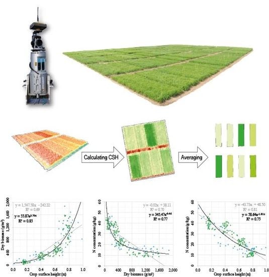
The time-of-flight scanner Riegl LMS-Z420i was used (near-infrared laser beam; beam divergence of 0.25 mrad; and measurement rate of up to 11,000 points/sec). Its field of view is up to 80° in the vertical and 360° in the horizontal direction and resolutions between 0.034° and 0.046° were used for this study. A Nikon D200 was mounted on top for colorizing the point clouds in the post-processing. The scanner was mounted on a hydraulic platform of a tractor (sensor height ~4 m above ground). During each campaign, the field was scanned from its four corners to lower shadowing effects and to attain an almost uniform spatial coverage. The coordinates of all scan positions were measured with the RTK DGPS system Topcon HiPer Pro. The position of a highly reflective cylinder arranged on a ranging pole was measured with the DGPS system and detected in each scan. An exact georeferencing and co-registration can thus be achieved with the DGPS-derived coordinates of the scan positions.

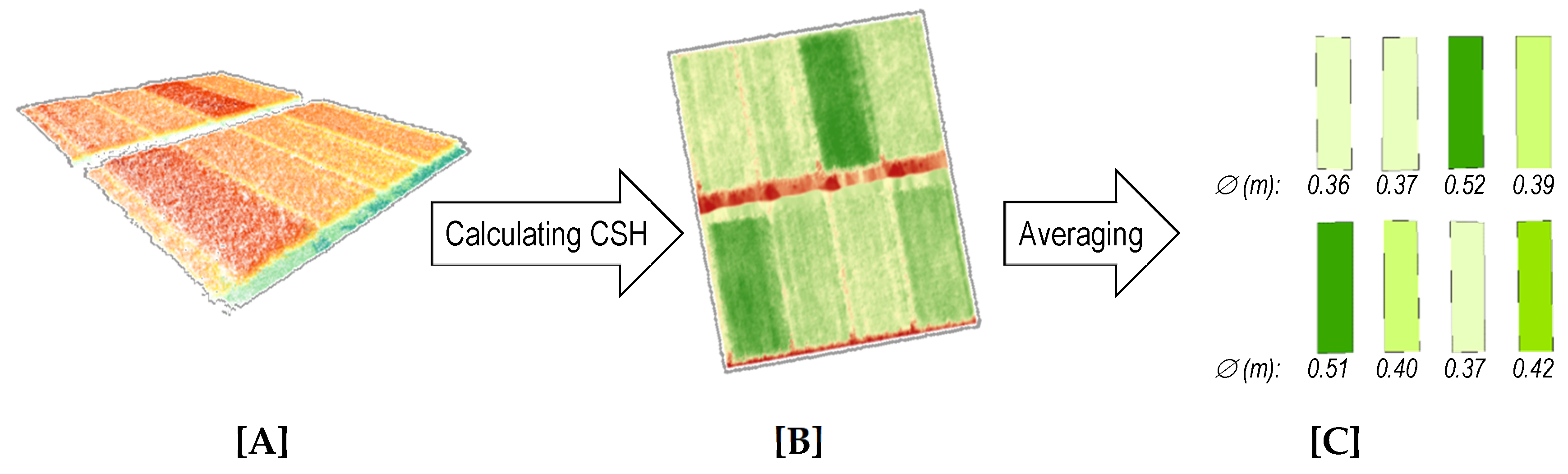
The main steps of the TLS data processing can be summarized to merging and cleaning of the point clouds, filtering of the highest points, which are regarded as crop canopy, and spatially resolved calculation of CSH. Crop surface models (CSMs), which represent the crop surface, were established. Crop surface height (CSH) is then calculated by spatially subtracting the digital terrain model (DTM) height from the CSM. A detailed description is given by Tilly et al. [60]. The result is a raster data set for each campaign with pixel-wise stored CSH. The CSH was averaged plot-wise to achieve a common spatial base with the other measurements (Figure 1).

2.1.2. Spectral Measurements

The ASD^® FieldSpec3 was used (measurement range from 350 to 2500 nm; sampling interval of 1.4 nm and 2 nm in visible-near-infrared and short-wave infrared, respectively; spectra are resampled to 1 nm resolution). A cantilever with a pistol grip was used to avoid shadows and a water level ensured a nadir view. Samples were taken from 1 m above canopy and no fore optic was used. Thus, the field of view was 25°, resulting in a circular footprint area with a radius of ~22 cm on the canopy. Six positions were taken for each plot and averaged for the analysis. Ten measurements per position were carried out and instantly averaged. The spectrometer warmed up for at least 30 min prior to measurements. It was calibrated with a spectralon calibration panel every 10 min or after illumination change. Measurements were carried out around noon to ensure the sun was at its highest.

In the post-processing, six VIs were calculated by Tilly et al. [65] for estimating biomass. These VIs were now further investigated regarding their relation to N concentration. The NIR-based simple ratio index R₇₆₀/R₇₃₀ was added for this study, as it was powerful for indicating the N status of wheat [40] and performed well for grain yield prediction with similar cultivars of spring barley as the here investigated [73]. The formulas of the VIs are given in

Table 1. Vegetation indices. Table modified from Tilly et al. [65].

Wave-Length Domains	Vegetation Index	Formula	References
NIR	GnyLi	$\left(R900\times R1050-R955\times R1220\right)/(R900\times R1050+R955\times R1220)$	[74]
	NRI	$\left(R874-R1225\right)/\left(R874+R1225\right)$	[75]
	R760/R730	$R760/R730$	[40]
VISNIR	NDVI	$\left(R798-R670\right)/\left(R798+R670\right)$	[76]
	RDVI	$\left(R798-R670\right)/\left(\sqrt{R798+R670}\right)$	[77]
	REIP	$700+40*\frac{\left(\frac{R670+R780}{2}\right)-R700}{R740-R700}$	[78]
VIS	RGBVI	$(R_{green}{}^2-R_{blue}\times R_{red})/(R_{green}{}^2+R_{blue}\times R_{red})$	[59]

. Different wavelength domains were covered by choosing two VIs in the near-infrared (NIR), three VIs in the visible-near-infrared (VISNIR), and one VI in the visible (VIS) domain.

2.1.3. Reference Measurements

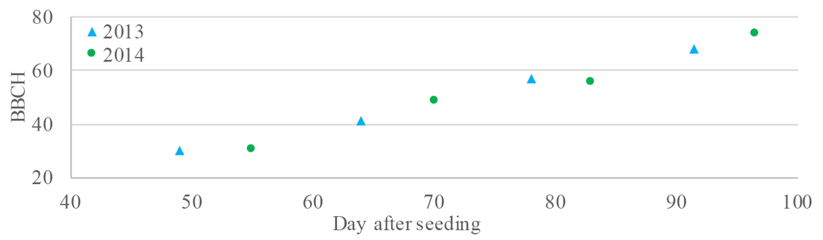
The BBCH scale was used to describe phenological stages and steps of plant development (Acronym BBCH is derived from the funding members: Biologische Bundesanstalt (German Federal Biological Research Centre for Agriculture and Forestry), Bundessortenamt (German Federal Office of Plant Varieties), and Chemical Industry) [79,80]. The campaign-wise averaged BBCH codes are plotted against day after seeding (DAS) in Figure 2. According to these codes, the campaigns covered the main vegetative phase, between stem elongation (Code 31) and end of fruit development (Code 79). In each campaign, the height of ten plants per plot was measured and averaged. The main stem height including ears was measured. Thin awns were excluded, as it is unlikely that they are captured by the laser scanner. In the defined sampling area of each plot, the aboveground biomass of a 0.2 × 0.2 m square was destructively taken each time and used to determine dry biomass in the laboratory. Each plant was previously divided into its individual organs (stem, leaf, and ear) and separately treated.

The dry biomass of the individual plant organs was further used for determining N concentration with the elemental analyzer vario EL cube [81]. For each plot, 2 to 3 mg dry biomass from stem, leaf, and ear were pulverized and homogenized. Each sample was catalytically combusted at 950 °C. The gas is separated through selective trap columns for determining the elemental composition by a thermoconductivity detector. The values of the stem, leaf, and ear samples were combined and averaged for each plot. The values of the entire plant were used in this first approach, as the entire crop surface and hence the whole plant is captured by the laser scanner. A brief overview about the values of individual plant organs will be given.

2.2. Estimation Models

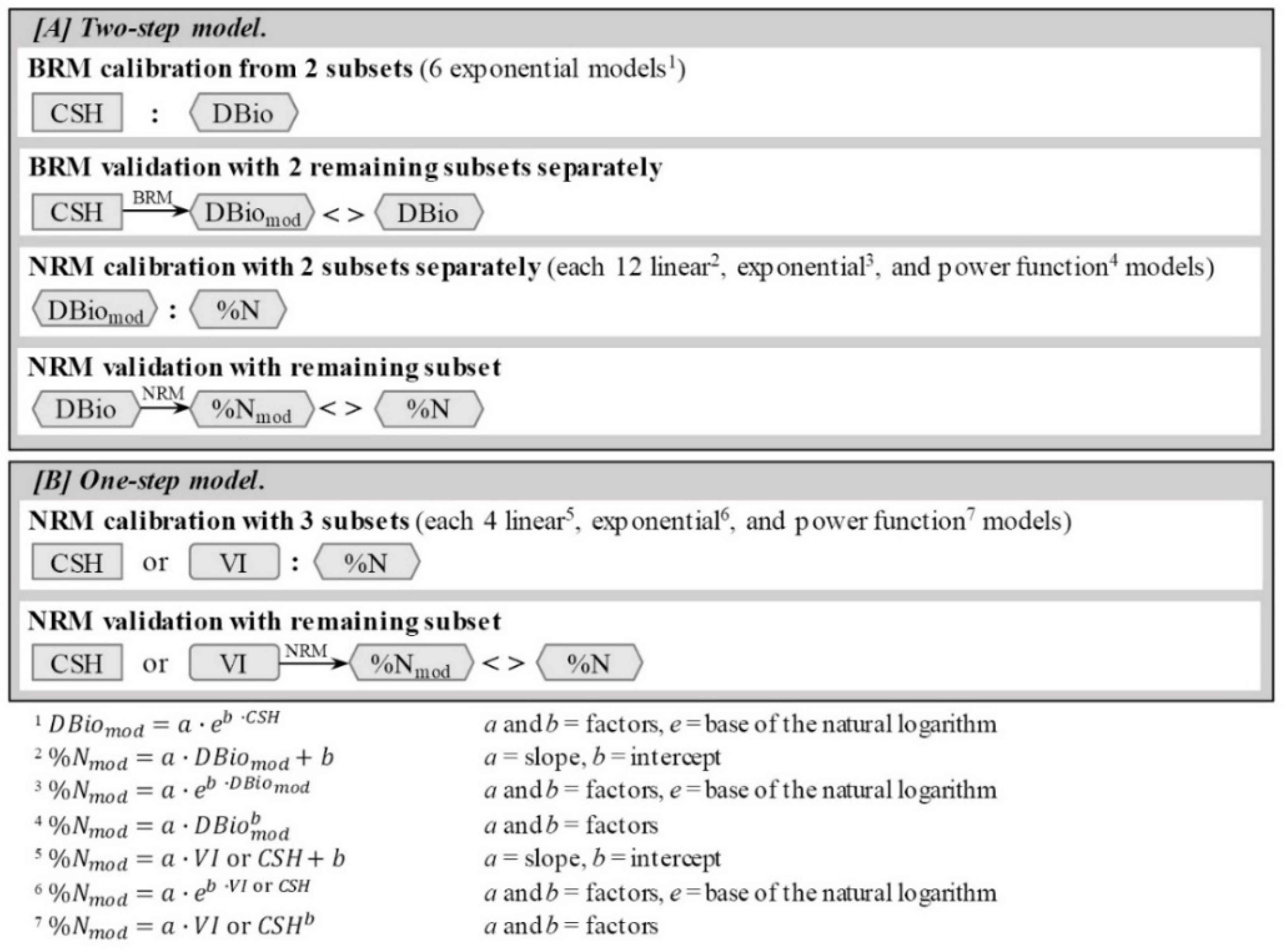
This study aims at investigating whether the crop-specific indirect link between structural traits and crop N concentration (%N) can be used for robust estimations at field scale. The data set was split into four subsets for a leave-one-out cross validation. All possible combinations of the subsets for calibration and one subset for validation were calculated. For a first model run, subset 1 contained the data sets of all campaigns from 2013 (n = 48). Each other subset contained the measurements of all campaigns from one repetition from 2014 (each n = 48). For a second and third model run, the data sets were split according to the levels of N fertilization, reducing the number of values per subset for each of these runs (n = 24).

Dry biomass (DBio) was first investigated as potential estimator for %N, based on the allometric relation between DBio and %N. A two-step model was designed as shown in Figure 3 [A]. The first step of the model aims at determining DBio from crop surface height (CSH). An exponential biomass regression model (BRM) was calibrated from two subsets, since this performed best for the observed period of the growing season [65]. DBio of the other two subsets was then separately determined and validated. The determined values are hereinafter referred to as DBio_mod. In the second step, one subset of DBio_mod and %N was used for calibrating a nitrogen regression model (NRM). As NRMs are newly investigated here, linear, exponential, and power function models were established. These NRMs were then applied to the remaining subset and validated. All calibrations were evaluated with the coefficient of determination (R_C²). The formula is given in (1). For each validation, besides the coefficient of determination (R_V²), the root mean square error (RMSE), and relative RMSE (rRMSE) were determined. The formulas are given in (2) to (4). All statistics are calculated for each run.

$$R_c^2={\left(\frac{{{\displaystyle \sum }}_{i=1}^n\left(x-\overline{x}\right)\left(y-\overline{y}\right)}{\sqrt{{{\displaystyle \sum }}_{i=1}^n{\left(x-\overline{x}\right)}^2{{\displaystyle \sum }}_{i=1}^n{\left(y-\overline{y}\right)}^2}}\right)}^2$$

(1)

where x refers to the estimator (CSH, DBio_mod, or VI) and y refers to the value which is estimated (DBio or %N).

$$R_v^2={\left(\frac{{{\displaystyle \sum }}_{i=1}^n\left(x-\overline{x}\right)\left(y-\overline{y}\right)}{\sqrt{{{\displaystyle \sum }}_{i=1}^n{\left(x-\overline{x}\right)}^2{{\displaystyle \sum }}_{i=1}^n{\left(y-\overline{y}\right)}^2}}\right)}^2$$

(2)

where x refers to the estimated values (DBio or %N) and y refers to the measured values (DBio or %N).

$$RMSE=\sqrt{\frac{{{\displaystyle \sum }}_{i=1}^n{\left(x_i-y_i\right)}^2}{n}}$$

(3)

where x refers to the estimated values, y refers to the measured values, and n is the number of samples.

$$rRMSE=\frac{RMSE}{\overline{M}}$$

(4)

where $\bar{M}$ is the across season mean value of the validation subset (DBio or %N).

Considering the physiological principles of plant responses to light competition, CSH is suggested as potential estimator for crop N status. Similar to the two‑step model, linear, exponential, and power function NRMs were established as one-step model (Figure 3 [B]). As only one subset was needed for the validation, three subsets were used for the calibration. Again, three model runs were carried out, for the entire data set and for the common and reduced level of N fertilization. The calibrations were evaluated by the R_C² and the validations by the R_V², RMSE, and rRMSE.

In addition, NRMs based on spectral data were established. In a pre‑test, the R² was calculated for each of the seven VIs vs. %N based on linear, exponential, and power function regressions. Based on the results, VIs were selected for the further considerations in the one‑step model. The model design is equal to the NRMs based on CSH (Figure 3 [B]).

2.3. Relationship Between Crop Traits and Plant Organs

In this first approach DBio and %N of the entire plant were used for the estimation models. Nonetheless, a brief look is taken at the relationship between the estimators and the individual plant organs. As outlined in the introduction, N is required by different plant organs depending on the growing stage. The competing for light among neighboring plants influences the N dilution [19,69], which is observable in various environments [82,83]. Scatterplots of CSH or VI vs. DBio and %N per plant organ were established to get a first impression. Furthermore, ear DBio was plotted against stem %N and leaf %N, since these storages are important for the ear and grain development.

3. Results

3.1. Crop Traits

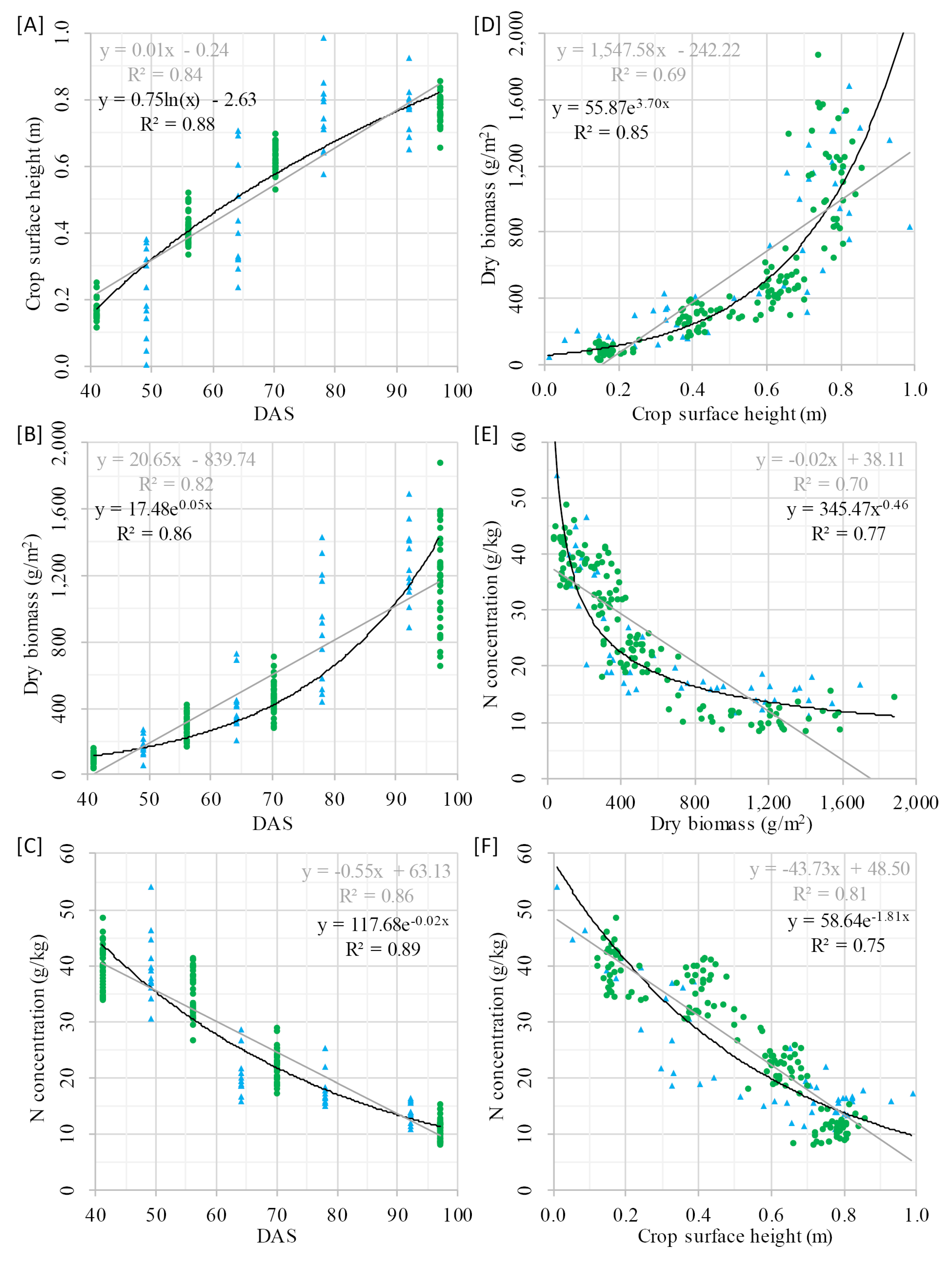
The following is a brief description of the captured crop traits.

Table 2. Statistics for the plot-wise averaged crop surface height (CSH), the destructively taken dry biomass (DBio), and nitrogen concentration (%N) measured in the laboratory. The values were calculated for subset 1 of 2013 and subsets 2, 3, and 4 of 2014 (DAS: Day after seeding; n: number of samples; mean: mean value; SD: standard deviation).

	DAS	Subset	n	CSH (m)		DBio (g/m2)		%N (g/kg)
				Mean	SD	Mean	SD	Mean	SD
2013	49	1	12	0.22	0.13	168.31	59.11	39.91	6.19
	64	1	12	0.46	0.17	415.31	152.51	20.56	3.73
	78	1	12	0.76	0.11	883.38	343.55	17.83	2.99
	92	1	12	0.78	0.07	1258.88	229.69	14.04	1.83
Mean				0.56	0.12	681.47	196.22	23.09	3.68
2014	41	2	12	0.17	0.03	86.69	31.22	39.94	3.82
	41	3	12	0.17	0.03	100.81	24.29	40.79	3.96
	41	4	12	0.17	0.03	79.54	26.14	39.37	3.78
	56	2	12	0.41	0.04	304.02	63.80	35.51	4.45
	56	3	12	0.42	0.05	290.90	77.10	35.69	3.94
	56	4	12	0.41	0.05	274.56	61.47	35.13	3.89
	70	2	12	0.63	0.03	487.73	82.10	22.02	3.11
	70	3	12	0.64	0.04	482.81	102.39	22.04	2.41
	70	4	12	0.62	0.04	425.95	107.53	23.07	2.69
	97	2	12	0.76	0.04	1247.56	285.68	11.13	2.13
	97	3	12	0.79	0.04	1138.10	296.94	11.33	1.86
	97	4	12	0.77	0.04	1113.50	263.13	10.73	1.62
Mean				0.50	0.04	502.68	118.48	27.23	3.14

shows the statistics of CSH, DBio, and %N. The values were calculated for the four campaigns of 2013, acting as subset 1 in the model design, and for the four campaigns of 2014 separately for subset 2 to 4. The subsets show similar patterns within each growing stage and comparable developments across the growing season. All values are additionally plotted against DAS in Figure 4 [A] to [C]. As a first approximation, the temporal development of all crop traits can quite good be explained by a linear trend (R²: 0.82–0.86). Better results can be achieved with a logarithmic function for CSH (R²: 0.88) and exponential functions for DBio (R²: 0.86) and %N (R²: 0.89). DBio is plotted against CSH in Figure 4 [D]. The relation between these traits was intensively discussed by Tilly et al. [65]. Considering the aim of this study, %N is plotted against DBio in Figure 4 [E] and against CSH in Figure 4 [F]. A linear regression explains the trend of DBio vs. %N quite well (R²: 0.70), but a power function works better (R²: 0.77). For CSH vs. %N the linear trend fits slightly better (R²: 0.81) then the exponential one (R²: 0.75). These values confirm the quality of the obtained data. The rather good link of %N to DBio and CSH should be noted, which supports the idea of using the indirect link for the estimation models.

3.2. Nitrogen Estimation

A two-step model was designed for investigating whether the indirect link between CSH, DBio, and %N can be used for estimating %N from structural traits. The reason for this assumption was that %N is negatively related to DBio, which, in turn, can be estimated from CSH. Further one-step models based on CSH and VIs were established for comparison.

3.2.1. Two-Step Models

In the first step, two subsets of CSH and DBio were used for calibrating the BRM and applied to the other two subsets, separately. 18 exponential BRMs were established, as every possible subset combination was calculated in three runs. The mean values for the calibration and validation are given in

Table 3. Summarized mean values for biomass regression models (Calibration: R_C²: coefficient of determination; Validation: R_V²: coefficient of determination, RMSE: root mean square error (g/m²), rRMSE: relative root mean square error; Entire: entire data set; Common: common N fertilization; Reduced: reduced N fertilization). The statistics for each possible subset combination are shown in the appendix (Table A1).

	RC2	RV2	RMSE	rRMSE
Entire	0.86	0.74	238.00	0.43
Common	0.86	0.81	213.81	0.40
Reduced	0.87	0.72	256.93	0.45

, summarized per model run. The statistics for each possible subset combination are shown in the appendix (

Table A1. Statistics for each run of the biomass regression models (Calibration: R_C²: coefficient of determination; Validation: R_v²: coefficient of determination, RMSE: root mean square error (g/m²), rRMSE: relative root mean square error).

Calibration Subset	Validation Subset	RC2	RV2	RMSE	rRMSE
Entire data set
1 and 2	3	0.83	0.79	189.74	0.38
1 and 2	4	0.83	0.75	204.09	0.43
1 and 3	2	0.84	0.81	232.62	0.44
1 and 3	4	0.84	0.75	207.14	0.44
1 and 4	2	0.81	0.81	229.79	0.43
1 and 4	3	0.81	0.79	190.90	0.38
2 and 3	1	0.90	0.61	322.25	0.47
2 and 3	4	0.90	0.75	202.88	0.43
2 and 4	1	0.89	0.60	343.49	0.50
2 and 4	3	0.89	0.79	191.64	0.38
3 and 4	1	0.89	0.61	313.03	0.46
3 and 4	2	0.89	0.81	228.41	0.43
Common N fertilization
1 and 2	3	0.80	0.89	148.80	0.33
1 and 2	4	0.80	0.79	196.42	0.42
1 and 3	2	0.82	0.78	278.95	0.53
1 and 3	4	0.82	0.78	205.86	0.44
1 and 4	2	0.80	0.79	260.68	0.49
1 and 4	3	0.80	0.89	133.74	0.29
2 and 3	1	0.91	0.78	241.05	0.36
2 and 3	4	0.91	0.79	192.90	0.41
2 and 4	1	0.91	0.79	227.57	0.34
2 and 4	3	0.91	0.91	140.50	0.31
3 and 4	1	0.92	0.78	261.10	0.39
3 and 4	2	0.92	0.79	278.15	0.53
Reduced N fertilization
1 and 2	3	0.85	0.77	220.80	0.40
1 and 2	4	0.85	0.72	203.87	0.43
1 and 3	2	0.86	0.85	171.58	0.32
1 and 3	4	0.86	0.72	204.06	0.43
1 and 4	2	0.83	0.85	184.17	0.35
1 and 4	3	0.83	0.77	231.74	0.42
2 and 3	1	0.92	0.53	412.87	0.60
2 and 3	4	0.92	0.71	210.76	0.44
2 and 4	1	0.88	0.52	371.16	0.54
2 and 4	3	0.88	0.76	322.87	0.58
3 and 4	1	0.89	0.53	388.46	0.56
3 and 4	2	0.89	0.86	160.78	0.30

). As comparative value for the RMSE, it is referred to the across‑season mean DBio of 681.47 g/m² and 502.68 g/m² for 2013 and 2014, respectively (Table 2). The differences between the model runs are negligible with quite high mean R_C² values of 0.86–0.87. In the validation, the run with the commonly fertilized plots performed slightly better (R_V²: 0.81). The other runs yielded comparable good results (R_V²: 0.74 and 0.72 for the entire data set and the reduced fertilized plots, respectively).

In the second step, one subset of DBio_mod and %N was used for calibrating the NRM. The remaining subset was used for the validation. NRMs based on linear, exponential, and power function regressions were calculated for investigating the type of regression between DBio and %N. 36 NRMs were established, since this step is again performed for every possible subset combination in three runs. The mean values are given in

Table 4. Summarized mean values for nitrogen regression models (NRMs) based on two-step models (Calibration: R_C²: coefficient of determination; Validation: R_V²: coefficient of determination, RMSE: root mean square error (g/kg), rRMSE: relative root mean square error; Entire: entire data set; Common: common N fertilization; Reduced: reduced N fertilization). The statistics for each possible subset combination are shown in the appendix (Table A2).

	Linear NRM				Exponential NRM				Power Function NRM
	RC2	RV2	RMSE	rRMSE	RC2	RV2	RMSE	rRMSE	RC2	RV2	RMSE	rRMSE
Entire	0.77	0.71	7.90	0.31	0.76	0.81	7.32	0.28	0.76	0.71	8.75	0.33
Common	0.82	0.69	8.10	0.30	0.84	0.80	6.96	0.25	0.80	0.70	10.05	0.36
Reduced	0.76	0.76	8.32	0.35	0.75	0.82	7.67	0.31	0.76	0.74	7.44	0.30

. The statistics for each possible subset combination are shown in the appendix (

Table A2. Statistics for each run of the nitrogen regression models (NRMs) based on two-step model. (Calibration: R_C²: coefficient of determination; Validation: R_V²: coefficient of determination, RMSE: root mean square error (g/kg), rRMSE: relative root mean square error).

		Linear NRM				Exponential NRM				Power Function NRM
Calibration Subset	Validation Subset	RC2	RV2	RMSE	rRMSE	RC2	RV2	RMSE	rRMSE	RC2	RV2	RMSE	rRMSE
Entire data set
3	4	0.88	0.79	5.97	0.22	0.88	0.86	6.86	0.25	0.80	0.65	12.90	0.48
4	3	0.88	0.77	6.40	0.23	0.87	0.85	6.11	0.22	0.77	0.73	7.71	0.28
2	4	0.88	0.79	7.18	0.27	0.87	0.86	5.49	0.20	0.77	0.62	15.14	0.56
4	2	0.88	0.74	8.61	0.32	0.87	0.86	6.35	0.23	0.77	0.60	13.84	0.51
2	3	0.88	0.77	7.46	0.27	0.87	0.87	6.00	0.22	0.77	0.73	7.57	0.28
3	2	0.88	0.74	7.49	0.28	0.88	0.85	6.10	0.22	0.80	0.62	11.61	0.43
1	4	0.44	0.79	6.98	0.26	0.46	0.86	8.94	0.33	0.72	0.72	6.34	0.23
4	1	0.87	0.54	9.66	0.42	0.87	0.65	7.00	0.30	0.77	0.79	5.08	0.22
1	3	0.42	0.77	7.84	0.29	0.44	0.85	10.30	0.38	0.72	0.79	7.52	0.27
3	1	0.86	0.54	8.58	0.37	0.87	0.65	6.70	0.29	0.80	0.79	4.87	0.21
1	2	0.44	0.74	7.30	0.27	0.46	0.85	9.62	0.35	0.72	0.69	7.25	0.27
2	1	0.87	0.54	11.34	0.49	0.87	0.73	8.37	0.36	0.77	0.79	5.22	0.23
Common N fertilization
3	4	0.88	0.79	6.20	0.22	0.90	0.87	6.61	0.23	0.82	0.64	11.66	0.41
4	3	0.95	0.74	6.25	0.22	0.95	0.82	7.49	0.26	0.82	0.73	8.08	0.28
2	4	0.93	0.79	7.31	0.26	0.93	0.89	5.50	0.19	0.80	0.62	17.09	0.61
4	2	0.95	0.71	11.42	0.40	0.95	0.85	6.90	0.24	0.82	0.56	21.11	0.74
2	3	0.93	0.74	6.41	0.22	0.93	0.82	7.31	0.25	0.80	0.74	7.37	0.25
3	2	0.88	0.71	8.84	0.31	0.90	0.83	6.60	0.23	0.82	0.60	15.63	0.55
1	4	0.56	0.79	5.63	0.20	0.59	0.87	6.73	0.24	0.77	0.72	6.74	0.24
4	1	0.94	0.53	10.72	0.43	0.96	0.67	6.99	0.28	0.82	0.79	5.85	0.24
1	3	0.54	0.74	6.97	0.24	0.57	0.82	8.56	0.30	0.77	0.78	8.51	0.29
3	1	0.85	0.53	8.38	0.34	0.89	0.67	6.52	0.26	0.82	0.80	5.33	0.22
1	2	0.56	0.71	7.48	0.26	0.59	0.83	7.35	0.26	0.77	0.67	7.51	0.26
2	1	0.92	0.53	11.62	0.47	0.94	0.67	6.95	0.28	0.80	0.79	5.67	0.23
Reduced N fertilization
3	4	0.93	0.80	5.58	0.21	0.92	0.85	7.19	0.28	0.83	0.64	11.43	0.44
4	3	0.85	0.81	6.78	0.26	0.82	0.89	4.77	0.18	0.75	0.74	7.37	0.28
2	4	0.90	0.80	6.64	0.26	0.89	0.84	5.32	0.21	0.79	0.63	12.71	0.49
4	2	0.85	0.84	5.25	0.20	0.82	0.89	5.28	0.21	0.75	0.68	7.97	0.31
2	3	0.89	0.81	9.60	0.37	0.89	0.89	5.66	0.22	0.79	0.73	7.73	0.30
3	2	0.93	0.84	5.35	0.21	0.92	0.88	6.06	0.24	0.83	0.68	7.66	0.30
1	4	0.38	0.80	7.98	0.31	0.38	0.76	17.15	0.66	0.65	0.72	5.85	0.23
4	1	0.84	0.58	8.05	0.38	0.82	0.69	6.41	0.30	0.75	0.85	3.81	0.18
1	3	0.37	0.81	7.90	0.30	0.37	0.89	10.66	0.41	0.65	0.80	8.40	0.32
3	1	0.92	0.58	17.41	0.81	0.92	0.69	6.87	0.32	0.83	0.85	5.45	0.25
1	2	0.37	0.84	8.38	0.33	0.37	0.87	9.33	0.36	0.65	0.75	6.90	0.27
2	1	0.89	0.58	10.92	0.51	0.89	0.76	7.33	0.34	0.79	0.85	3.98	0.19

). As comparative value for the RMSE, it is referred to the across‑season mean %N values of 23.09 g/kg and 27.23 g/kg for 2013 and 2014, respectively (Table 2). The differences between the model runs are again almost negligible. The best results were achieved with the exponential NRM for the data set of the commonly fertilized plots (R_C²: 0.84 and R_V²: 0.80). The power function NRM for the entire data set performed weaker. However, these results are also far from poor with a mean R_C² of 0.76 and R_V² of 0.71. The RMSE is also similar for the linear and exponential NRM, but slightly higher for the power function NRM.

3.2.2. One-Step Models

Similar to the second step of the two‑step model, NRMs based on linear, exponential, and power function regressions were established with CSH as estimator. 12 NRMs were established, since the models are again performed for every possible subset combination in three runs. The mean values are given in

Table 5. Summarized mean values for nitrogen regression models (NRMs) based on crop surface height (Calibration: R_C²: coefficient of determination; Validation: R_V²: coefficient of determination, RMSE: root mean square error (g/kg), rRMSE: relative root mean square error; Entire: entire data set; Common: common N fertilization; Reduced: reduced N fertilization). The statistics for each possible subset combination are shown in the appendix (Table A3).

	Linear NRM				Exponential NRM				Power function NRM
	RC2	RV2	RMSE	rRMSE	RC2	RV2	RMSE	rRMSE	RC2	RV2	RMSE	rRMSE
Entire	0.81	0.82	5.05	0.19	0.76	0.78	5.84	0.22	0.60	0.58	15.81	0.58
Common	0.82	0.82	4.68	0.19	0.75	0.79	5.06	0.21	0.66	0.68	6.43	0.26
Reduced	0.83	0.85	4.89	0.18	0.78	0.80	6.17	0.23	0.58	0.63	21.53	0.84

. The statistics for each possible subset combination are shown in the appendix (

Table A3. Statistics for each run of the nitrogen regression models (NRMs) based on crop height (Calibration: R_C²: coefficient of determination; Validation: R_V²: coefficient of determination, RMSE: root mean square error (g/kg), rRMSE: relative root mean square error).

		Linear NRM				Exponential NRM				Power Function NRM
Calibration Subset	Validation Subset	RC2	RV2	RMSE	rRMSE	RC2	RV2	RMSE	rRMSE	RC2	RV2	RMSE	rRMSE
Entire data set
1, 2, and 3	4	0.80	0.85	4.51	0.17	0.75	0.77	5.55	0.21	0.59	0.65	7.19	0.27
1, 2, and 4	3	0.80	0.87	4.54	0.17	0.74	0.79	5.69	0.21	0.58	0.65	7.48	0.28
1, 3, and 4	2	0.80	0.84	4.74	0.18	0.75	0.76	5.76	0.21	0.59	0.63	7.49	0.28
2, 3, and 4	1	0.85	0.73	6.41	0.24	0.78	0.81	6.36	0.24	0.63	0.41	41.10	1.52
Common N fertilization
1, 2, and 3	4	0.81	0.89	3.98	0.14	0.77	0.80	5.20	0.18	0.56	0.68	7.54	0.27
1, 2, and 4	3	0.82	0.87	4.76	0.16	0.77	0.79	5.94	0.21	0.56	0.68	8.28	0.29
1, 3, and 4	2	0.82	0.86	4.30	0.15	0.77	0.76	5.72	0.20	0.56	0.63	7.77	0.27
2, 3, and 4	1	0.87	0.78	6.53	0.26	0.81	0.85	7.84	0.32	0.65	0.52	62.51	2.53
Reduced N fertilization
1, 2, and 3	4	0.81	0.84	4.36	0.17	0.74	0.77	5.24	0.20	0.67	0.64	7.06	0.27
1, 2, and 4	3	0.78	0.92	3.37	0.13	0.72	0.84	4.52	0.17	0.66	0.68	7.14	0.28
1, 3, and 4	2	0.81	0.87	4.54	0.18	0.74	0.80	5.18	0.20	0.67	0.66	6.99	0.27
2, 3, and 4	1	0.88	0.65	6.46	0.30	0.79	0.74	5.31	0.25	0.64	0.75	4.53	0.21

). As comparative value for the RMSE, it is again referred to Table 2. The differences between the three model runs are almost negligible. The best results were achieved with the linear NRMs (R_C²: 0.81–0.83 and R_V²: 0.82–0.85) followed by the exponential NRMs (R_C²: 0.75–0.78 and R_V²: 0.78–0.80). Slightly worse performed the power function NRMs (R_C²: 0.58–0.66 and R_V²: 0.58–0.68). The RMSE is again similar for the linear and exponential NRM, but slightly higher for the power function NRM.

As comparative data to the estimations from structural traits, the usability of the calculated VIs for estimating %N was investigated. The R² of each plot‑wise averaged VI vs. %N was calculated for each of the seven VIs based on a linear, an exponential, and a power function regression as a pre-test. Based on these results (

Table 6. Pre-test: Coefficient of determination (R²) between the plot-wise averaged vegetation indices and the nitrogen concentration.

	Linear	Exponential	Power Function
GnyLi	0.66	0.59	0.48
NDVI	0.11	0.06	0.06
NRI	0.68	0.61	0.47
RDVI	0.19	0.12	0.13
REIP	0.18	0.10	0.10
RGBVI	0.10	0.05	0.05
R760/R730	0.11	0.12	0.05

), four VIs were selected for further analysis. The GnyLi and NRI were chosen as they performed best (R²: 0.47–0.68). Even though the REIP and the R₇₆₀/R₇₃₀ yielded far poorer results (R²: 0.04–0.18), they were further investigated, as these VIs are known from literature for its usefulness for estimating %N [30,32,40]. The NDVI, RDVI, and RGBVI were neglected due to their poor performance (R²: 0.10–0.19).

Similar to the one‑step models based on CSH, NRMs based on linear, exponential, and power function regressions were established with GnyLi, NRI, REIP, and R₇₆₀/R₇₃₀ as estimators. The mean values are given in

Table 7. Summarized mean values for nitrogen regression models (NRMs) based on vegetation indices (Calibration: R_C²: coefficient of determination; Validation: R_V²: coefficient of determination, RMSE: root mean square error (g/kg), rRMSE: relative root mean square error; Entire: entire data set; Common: common N fertilization; Reduced: reduced N fertilization). The statistics for each possible subset combination are shown in the appendix (Table A4).

	Linear NRM				Exponential NRM				Power Function NRM
	RC2	RV2	RMSE	rRMSE	RC2	RV2	RMSE	rRMSE	RC2	RV2	RMSE	rRMSE
GnyLi
Entire	0.66	0.67	6.66	0.25	0.59	0.61	7.57	0.29	0.49	0.50	10.70	0.40
Common	0.66	0.67	6.73	0.24	0.61	0.59	8.12	0.29	0.46	0.47	11.46	0.41
Reduced	0.67	0.69	6.32	0.25	0.58	0.67	6.54	0.26	0.53	0.63	7.46	0.30
NRI
Entire	0.68	0.68	6.47	0.24	0.61	0.62	7.47	0.28	0.47	0.48	9.87	0.37
Common	0.68	0.68	6.58	0.24	0.63	0.60	7.90	0.29	0.45	0.46	10.30	0.37
Reduced	0.69	0.70	6.07	0.24	0.60	0.66	6.60	0.26	0.52	0.59	8.40	0.33
REIP
Entire	0.19	0.23	10.56	0.39	0.10	0.25	137.22	5.07	0.10	0.25	10.59	0.39
Common	0.28	0.33	10.25	0.37	0.18	0.35	88.71	3.47	0.19	0.35	10.12	0.37
Reduced	0.14	0.24	10.22	0.41	0.06	0.25	178.00	6.98	0.06	0.25	10.37	0.42
R760/R730
Entire	0.11	0.15	10.96	0.42	0.05	0.16	11.25	0.43	0.06	0.18	11.11	0.42
Common	0.18	0.24	10.63	0.38	0.11	0.26	10.74	0.39	0.03	0.17	13.06	0.52
Reduced	0.07	0.15	10.58	0.43	0.02	0.16	10.83	0.44	0.12	0.27	10.63	0.38

. The structure of the table is equal to Table 5. The statistics for each possible subset combination are shown in the appendix (

Table A4. Statistics for each run of the nitrogen regression models (NRMs) based on vegetation indices (Calibration: R_C²: coefficient of determination; Validation: R_V²: coefficient of determination, RMSE: root mean square error (g/kg), rRMSE: relative root mean square error).

		Linear NRM				Exponential NRM				Power Function NRM
Calibration Subset	Validation Subset	RC2	RV2	RMSE	rRMSE	RC2	RV2	RMSE	rRMSE	RC2	RV2	RMSE	rRMSE
GnyLi
Entire data set
1, 2, and 3	4	0.67	0.64	6.99	0.26	0.61	0.55	8.84	0.33	0.53	0.30	18.22	0.67
1, 2, and 4	3	0.66	0.68	6.77	0.25	0.59	0.60	7.75	0.28	0.48	0.51	8.75	0.32
1, 3, and 4	2	0.69	0.58	7.64	0.28	0.62	0.51	8.77	0.32	0.51	0.40	9.89	0.36
2, 3, and 4	1	0.63	0.76	5.24	0.23	0.54	0.79	4.91	0.21	0.43	0.77	5.94	0.26
Common N fertilization
1, 2, and 3	4	0.68	0.64	7.31	0.26	0.64	0.52	9.64	0.34	0.52	0.28	19.32	0.68
1, 2, and 4	3	0.66	0.68	6.77	0.23	0.60	0.58	7.84	0.27	0.45	0.48	9.14	0.32
1, 3, and 4	2	0.70	0.55	7.55	0.26	0.64	0.45	9.28	0.32	0.48	0.36	9.97	0.35
2, 3, and 4	1	0.61	0.82	5.29	0.21	0.55	0.81	5.75	0.23	0.40	0.77	7.39	0.30
Reduced N fertilization
1, 2, and 3	4	0.67	0.65	6.46	0.25	0.58	0.58	7.60	0.29	0.56	0.51	10.17	0.39
1, 2, and 4	3	0.66	0.68	6.48	0.25	0.58	0.63	7.26	0.28	0.54	0.55	7.99	0.31
1, 3, and 4	2	0.70	0.59	7.61	0.30	0.61	0.57	8.03	0.31	0.56	0.54	8.37	0.33
2, 3, and 4	1	0.63	0.83	4.74	0.22	0.53	0.89	3.27	0.15	0.47	0.90	3.31	0.15
NRI
Entire data set
1, 2, and 3	4	0.69	0.66	6.74	0.25	0.62	0.56	8.22	0.31	0.49	0.41	10.50	0.39
1, 2, and 4	3	0.67	0.71	6.45	0.24	0.61	0.61	7.68	0.28	0.47	0.46	9.11	0.34
1, 3, and 4	2	0.71	0.61	7.35	0.27	0.64	0.52	8.83	0.33	0.51	0.31	13.17	0.49
2, 3, and 4	1	0.65	0.74	5.33	0.20	0.58	0.78	5.14	0.19	0.42	0.75	6.69	0.25
Common N fertilization
1, 2, and 3	4	0.69	0.66	6.83	0.25	0.65	0.55	8.09	0.29	0.46	0.36	9.76	0.35
1, 2, and 4	3	0.67	0.68	6.66	0.23	0.62	0.57	8.01	0.28	0.44	0.41	9.39	0.32
1, 3, and 4	2	0.70	0.59	7.27	0.25	0.66	0.49	9.47	0.33	0.49	0.32	14.22	0.50
2, 3, and 4	1	0.64	0.80	5.59	0.23	0.59	0.80	6.05	0.24	0.40	0.73	7.84	0.32
Reduced N fertilization
1, 2, and 3	4	0.69	0.66	6.40	0.25	0.61	0.58	8.01	0.31	0.55	0.47	12.89	0.50
1, 2, and 4	3	0.67	0.73	5.96	0.23	0.59	0.65	6.91	0.27	0.51	0.55	7.96	0.31
1, 3, and 4	2	0.72	0.61	7.34	0.29	0.63	0.57	8.00	0.31	0.54	0.50	8.61	0.34
2, 3, and 4	1	0.66	0.78	4.60	0.21	0.56	0.85	3.46	0.16	0.46	0.86	4.14	0.19
REIP
Entire data set
1, 2, and 3	4	0.19	0.17	11.16	0.41	0.10	0.19	25.28	0.93	0.10	0.19	10.81	0.40
1, 2, and 4	3	0.20	0.15	10.94	0.40	0.11	0.17	12.91	0.48	0.11	0.17	11.57	0.43
1, 3, and 4	2	0.21	0.12	11.20	0.41	0.12	0.14	93.14	3.44	0.12	0.14	11.41	0.42
2, 3, and 4	1	0.14	0.47	8.94	0.33	0.06	0.49	417.55	15.42	0.06	0.50	8.58	0.32
Common N fertilization
1, 2, and 3	4	0.30	0.21	10.46	0.37	0.21	0.23	27.47	0.97	0.21	0.23	10.20	0.36
1, 2, and 4	3	0.31	0.19	11.44	0.39	0.21	0.20	29.25	1.01	0.21	0.20	11.35	0.39
1, 3, and 4	2	0.30	0.19	10.19	0.36	0.20	0.22	27.72	0.97	0.21	0.22	10.24	0.36
2, 3, and 4	1	0.19	0.73	8.91	0.36	0.11	0.74	270.41	10.94	0.11	0.75	8.70	0.35
Reduced N fertilization
1, 2, and 3	4	0.13	0.14	10.17	0.39	0.06	0.15	26.21	1.01	0.06	0.15	10.52	0.41
1, 2, and 4	3	0.14	0.14	10.93	0.42	0.07	0.15	11.07	0.43	0.07	0.15	11.37	0.44
1, 3, and 4	2	0.16	0.08	11.65	0.45	0.08	0.09	653.62	25.51	0.08	0.09	11.44	0.45
2, 3, and 4	1	0.11	0.60	8.15	0.38	0.04	0.62	21.11	0.98	0.04	0.61	8.15	0.38
R760/R730
Entire data set
1, 2, and 3	4	0.12	0.08	10.91	0.40	0.05	0.10	11.31	0.42	0.06	0.11	11.12	0.41
1, 2, and 4	3	0.13	0.08	11.48	0.42	0.06	0.09	12.09	0.44	0.07	0.10	11.97	0.44
1, 3, and 4	2	0.13	0.06	11.42	0.42	0.06	0.07	11.73	0.43	0.07	0.09	11.63	0.43
2, 3, and 4	1	0.07	0.39	10.04	0.43	0.02	0.40	9.87	0.43	0.03	0.42	9.72	0.42
Common N fertilization
1, 2, and 3	4	0.20	0.12	10.84	0.38	0.13	0.14	10.75	0.38	0.14	0.16	10.59	0.38
1, 2, and 4	3	0.21	0.11	11.27	0.39	0.12	0.12	11.55	0.40	0.13	0.13	11.51	0.40
1, 3, and 4	2	0.21	0.10	10.76	0.38	0.12	0.12	10.82	0.38	0.13	0.14	10.72	0.37
2, 3, and 4	1	0.11	0.65	9.64	0.39	0.05	0.66	9.82	0.40	0.06	0.67	9.70	0.39
Reduced N fertilization
1, 2, and 3	4	0.07	0.06	10.57	0.41	0.02	0.06	11.23	0.43	0.03	0.06	20.24	0.78
1, 2, and 4	3	0.08	0.06	11.02	0.42	0.02	0.06	11.59	0.45	0.03	0.07	11.58	0.45
1, 3, and 4	2	0.09	0.04	11.42	0.45	0.03	0.04	11.76	0.46	0.03	0.05	11.74	0.46
2, 3, and 4	1	0.05	0.46	9.34	0.44	0.01	0.47	8.75	0.41	0.01	0.49	8.66	0.40

). As it could be assumed from the pre-test, the R₇₆₀/R₇₃₀ and REIP showed the overall worst performance with mean R_C² of 0.02–0.18 and R_V² of 0.15–0.27 and R_C² of 0.06–0.28 and R_V² of 0.23–0.35, respectively. The GnyLi and NRI yielded better and among themselves comparable results. The differences between the model runs can again be neglected. Mean R_C² values between 0.45 and 0.68 were obtained with both VIs. The linear models performed best; closely followed by the exponential NRMs and the power function provided the worst results. A similar pattern can be stated for the validation. The linear NRMs showed the best performance with R_V² of 0.67–0.70. They are closely followed by the exponential ones (R_V²: 0.58–0.61). The power function models performed slightly weaker (R_V²: 0.47–0.63). For all VIs, the RMSE is again lower for the linear and exponential models than for the power function models.

3.3. Relationship Between Crop Traits and Plant Organs

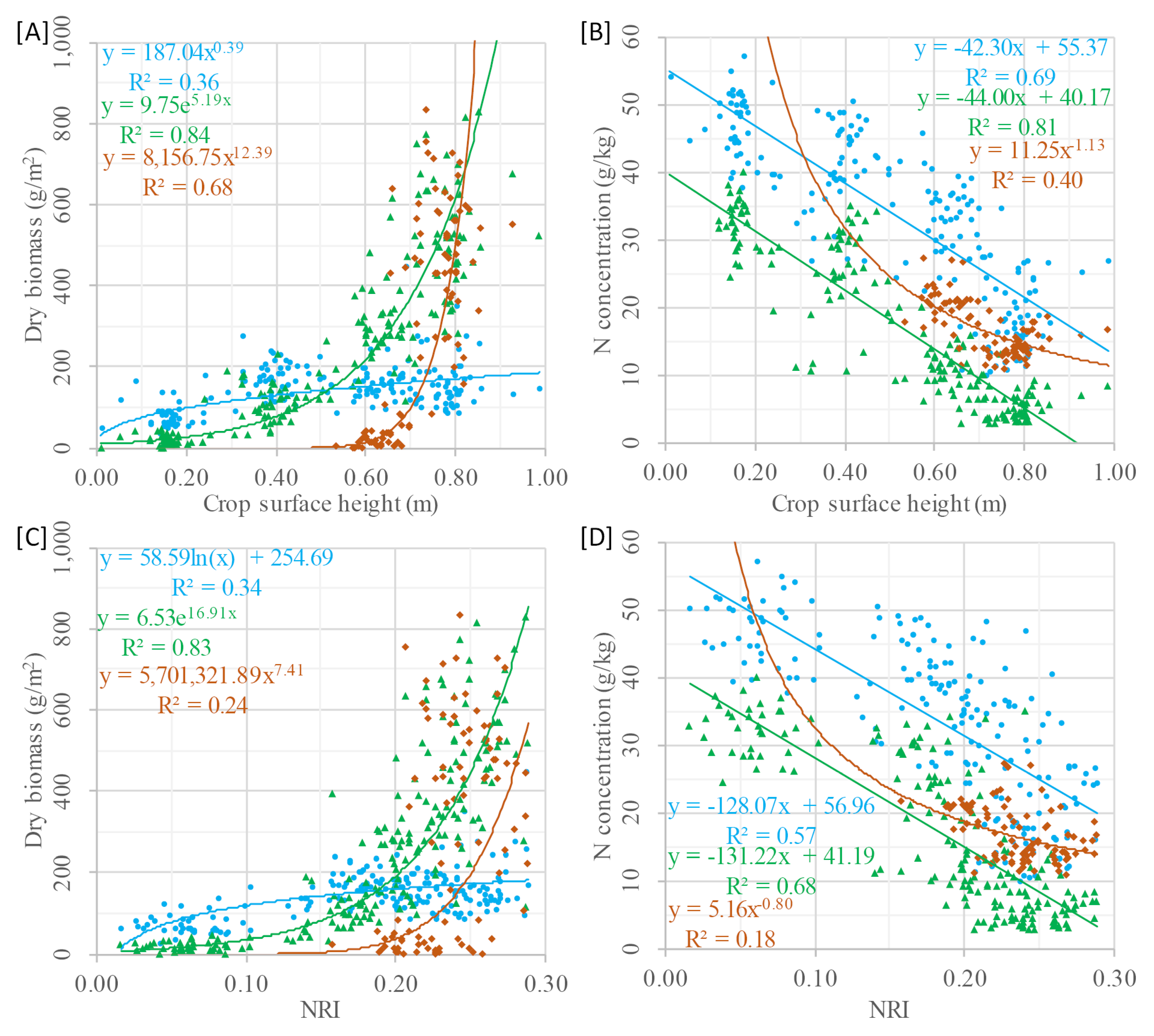
DBio and %N of the entire plant were used for the models in this first approach, as the entire crop surface and hence the whole plant is captured by the laser scanner. At this point, a brief look is thrown on the relation between the used estimators and individual plant organs. Figure 5 shows DBio [A] and %N [B] per plant organ plotted against CSH. It is rather obvious that stem DBio depends on CSH (R²: 0.84), whereas leaf DBio shows a weaker R² of 0.36. CSH and ear DBio show a moderate relation (R²: 0.68). From a plant physiological point of view, the stem has a key role in the plant growth process. While competing for light with their neighboring plants, a large stem length alias high CSH, accompanied by high biomass, supports the plant to place their leaves to the better-illuminated top layers. Furthermore, plants use stem N for the grain development [3]. As it can be seen in Figure 5 [B], stem %N is rather strong related to CSH (R²: 0.81). It is also visible that generally more N is allocated to the metabolic actives leaves in comparison to the stem. Even more interesting is, however, the similar negative slope of leaf %N and stem %N vs. CSH. All investigated VIs provided poorer results. As shown for the NRI in Figure 5 [C], slightly weaker values were achieved for stem DBio (R²: 0.34) and leaf DBio (R²: 0.83). Rather poor values can be stated for ear DBio (R²: 0.24). Considerably lower values were achieved for NRI vs. %N of the individual organs as shown in Figure 5 [D]. Only R² of 0.57, 0.68, and 0.18 were reached for stem, leaf, and ear %N, respectively.

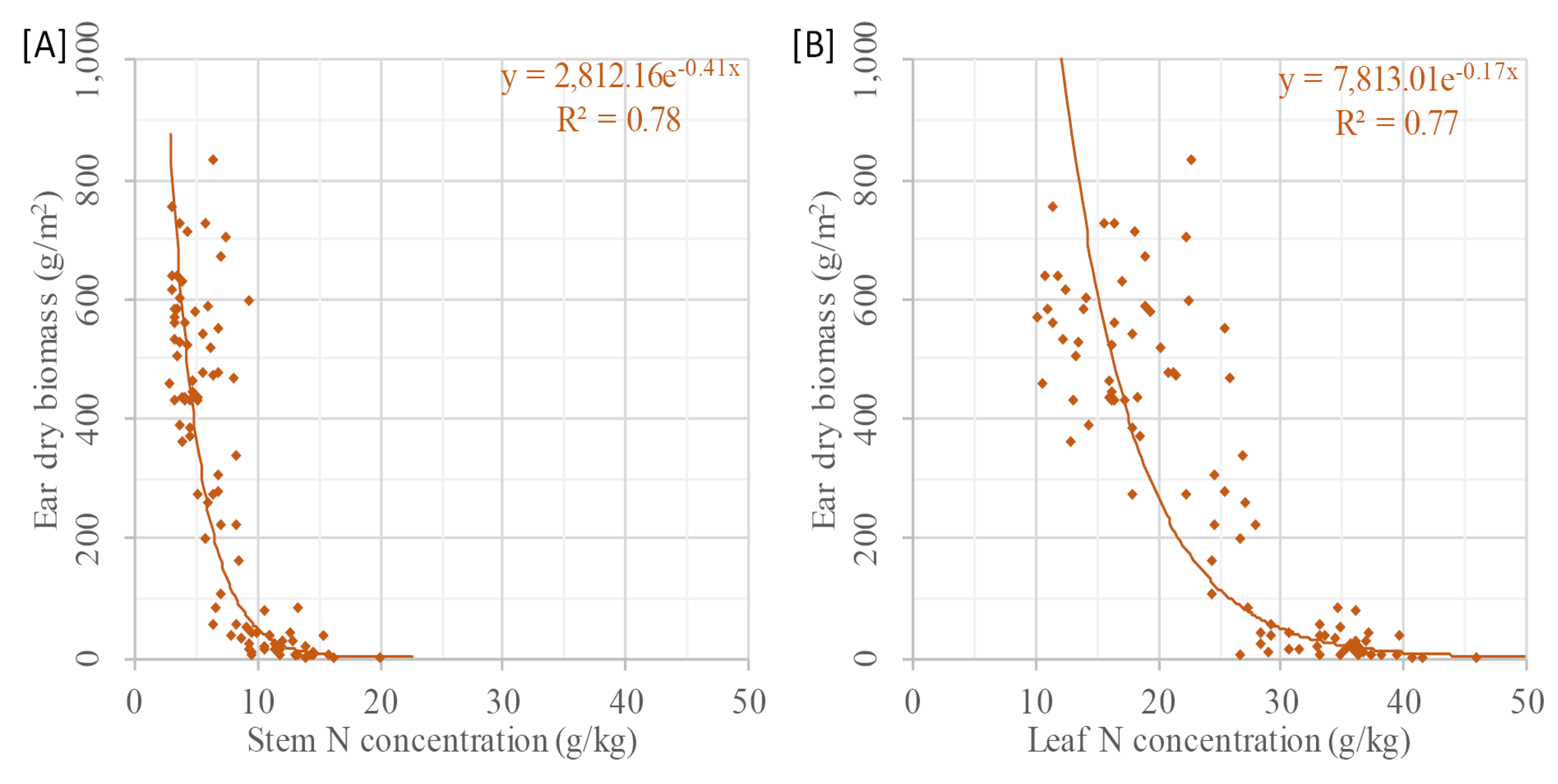
During the growing season, ear DBio can be used for quantitatively predicting the expected yield, which is most important for crop production. How well the grain develops depends on the available N, with stem N as main source, followed by leaf N, released through natural senescence, and soil N [3]. Since plants let their leaves die off if these sources are too low, a sufficient N storage can prevent this process, which would inhibit photosynthesis. During the early growing season, before ears are present, and where crop development can mainly be influenced, stem and leaf %N are hence most important. Ear DBio vs. stem %N and leaf %N are plotted in Figure 6 to investigate this relation. A slightly higher coefficient of determination was reached for stem %N (R²: 0.78) compared to leaf %N (R²: 0.77). Moreover, the scattering of the values is higher for leaf %N.

4. Discussion

A first investigation of crop-specific models based on structural traits for indirectly estimating N concentration (%N) at field scale can be stated as overall aim of this study. Crop biomass and %N are two of the most important traits under investigation in precision agriculture. The usability of TLS‑derived crop surface height (CSH) or rather plant height as estimator for biomass has been demonstrated by several authors [57,58,59,60,61,62,63]. An increasing number of studies on estimating biomass highlight the benefits of crop height as structural trait in comparison to spectral measurements [47,59,65]. In contrast, %N is commonly estimated from spectral data [4,31,32,33]. It is well known that N is negatively related to biomass during the growing season, which, in turn, can be estimated from CSH. Based on this indirect link, a two-step model was designed for determining DBio based on CSH in the first step, followed by estimating %N with a nitrogen regression model (NRM) from the determined DBio in the second step. In addition, CSH was examined as estimator in one‑step NRMs and similar NRMs based on VIs were established.

The development of CSH, DBio, and %N across the growing season showed that each crop trait has a certain pattern, which can be expressed with mathematic functions (R²: 0.82–0.89). The relation between DBio and %N can be expressed with a power function (R²: 0.77). Similar patterns were shown for winter barley [24] and corn [29]. That the allometric relation of %N vs. DBio during the vegetative growth can be expressed with a negative power function has early been recognized [20] and is the fundament of the NNI and NDC concept. As shown in Figure 4 [F], CSH vs. %N appears to be linearly (R²: 0.81) or exponentially (R²: 0.75) related, which supports the idea of using this structural trait as estimator for the N status of crops. Unfortunately, no comparable studies at field scale were found.

The applicability of biomass regression models (BRMs) based on CSH was demonstrated by Tilly et al. [65]. In contrast, crop-specific NRMs are newly developed in this study and thus examined more closely with linear, exponential, and power functions. Since the NRMs of all approaches were similarly designed, the results can well be compared. A point in common of all NRMs is that only negligible differences between the three runs could be observed. This might be explained by the minor difference between the fertilizer treatments of only 40 kg/ha. In contrast, in the literature differences of 70 to 220 kg/ha can be found for common field experiments [30,41,73,84] or single experiments with extremely high rates of up to 420 kg/ha [30].

Spectral approaches for determining %N are presented in different studies [30,31,32,33,34]. In these studies, R² values between 0.50 and 0.80 were reached for different crops. The best performing VI in this study reached comparable results (R² < 0.70). Good results achieved with the R₇₆₀/R₇₃₀ and REIP in other studies [30,32,40] could not be confirmed here (R_V² < 0.35). Even though these VIs will be excluded from the model comparison, some explanations for their weak performance should be formulated. First, all other studies investigated wheat not barley. Furthermore, Erdle et al. (2011) [40] and Baresel et al. [30] investigated measurements within one growing stage and used bidirectional radiometer or active sensors. Similar to this study, Li et al. [32] investigated different growing stages with a field spectrometer but obtained beside the quite good R² of 0.55 also weak results of 0.21 for the REIP. It can be summarized that the R₇₆₀/R₇₃₀ and REIP might be suitable for estimating crop %N. It should, however, be further investigated how prone these VIs are to effects such as saturation [37], multiangular reflection [85], leaf inclination angle [43], or general atmospheric conditions. Further research should involve additional VIs, which were investigated for N content and N uptake, such as the red edge-based canopy chlorophyll content index [86] or the optimum multiple narrow band reflectance model [31]. Another approach that can be found in the literature are contour plot analyses. Conclusions of two studies are, however, that it is challenging to obtain the necessary information with two-band VIs due to the N dilution effect [31] and that it will be difficult to develop a simple sensor that can determine the N concentration of plants with two or three bands for different growth stages [32]. The presented approach based on structural data shall introduce an alternative method.

The power function produced the poorest results of the three function types, with the lowest R² and highest RMSE values. Furthermore, the weakest results were achieved with the two remaining VIs. For both VIs, best results were obtained with linear models, whereas the NRI performed slightly better (R_V²: 0.68–0.70) than the GnyLi (R_V²: 0.67–0.69). The NRMs based on DBio_mod yielded better results and performed best with exponential functions (R_V²: 0.81–0.82). The best and most robust results were obtained with the NRMs based on CSH (R_V²: 0.78–0.85). It should be further investigated whether the fusion of CSH and VIs in multivariate models improves the estimation, as it was observed for the BRMs [65]. The benefit of the fusion of spectral and structural traits are also highlighted by other studies. The yield prediction of drought stressed barley for example could be improved [73]. Acquiring 3D and spectral data with one sensor could therefore be worthwhile, which might be realizable with recently emerging hyperspectral laser scanners [87]. First approaches of estimating rice leaf %N from multispectral and hyperspectral scanners can already be found [88,89]. These studies, however, only investigated the spectral information. Further research on the fusion of structural and spectral traits is required.

Quality, usability, and robustness of models can be assessed according to their accuracy and precision. Widely used metrics are the R_C², R_V², RMSE, and rRMSE. In case of the NRMs, R_C² shows if CSH-based DBio models, CSH or VIs can express variations of %N and hence if it is a suitable indicator. R_V² shows whether this relation is robust and transferable to independent data. It can well be used to compare the models among each other. RMSE and rRMSE are suitable for comparing the precision between the models. However, for evaluating the accuracy of NRMs for estimating %N, actual measurements must be considered. A major issue of across‑season estimations is the very varying %N. The rRMSE refers to the across‑season mean value, which can obviously hardly be used as reliable reference for the accuracy of the NRM at a certain point in time. As shown for the BRMs [90], more credible values can be obtained with campaign‑wise separated analyses. Similar results are very assumable for the NRMs, which requires further research. The validity of the RMSE for time‑specific models must be further investigated to evaluate the usability of the approach for site-specific management. Beyond that, studies are needed on the transferability of the models to other field locations, years, or crops. Good results have already been achieved for the transferability of BRMs for paddy rice [91]. However, it is known from the literature that the relationship between biomass and nitrogen is very different depending on the crop [24,92]. Accordingly, it can be assumed that NRMs must be calibrated crop-specific, as is the case for approaches with the nitrogen nutrition index (NNI). Novel machine learning approaches and algorithms, summarized as artificial intelligence, should also be taken into account for estimating crop traits [93,94,95]. Approaches of estimating grass sward biomass [96], quantifying rice N status [97], or monitoring wheat leaf %N [98] can already be found. As mentioned, an important point for site-specific management is the applicability of models at certain stages within the growing season. Analyses within one campaign were not very reliable with the available data set, due to the amount of data. Accordingly, further analyses with more extensive data sets are desirable for verifying the time-specific applicability of this approach.

The brief look at the relation between the estimators and individual plant organs suggests that CSH might be useful for estimating stem DBio and %N. The observed relation between CSH and leaf %N supports findings of Yin et al. [99]. They found a good relationship between plant height of corn and leaf %N. Beside the known fact that more N is allocated to the metabolic actives leaves than to the stem, a similar negative slope of leaf %N and stem %N vs. CSH was found. As the quantification of metabolic and structural N demand of individual plant organs is required for example for growth simulation models [5], further research on this is desirable. Moreover, this research can make an important contribution to understand the processes and traits, which are involved in the growth and N cycle of plants. For some crops, such as wheat, barley, and maize, the pre-anthesis ear and stem growth are somehow interlinked [100]. From the rather good relation between ear DBio and stem %N (R²: 0.78) or leaf %N (R²: 0.77), it can be interpreted that these individual plant organs might be useful for yield approximations during the growing season. Further research on this is required.

Considering finally the applicability in the field, the main benefits of capturing structural traits in comparison to spectral measurements were stated in the introduction. A main disadvantage of acquiring spectral data with handheld spectrometers is the limitation to several discrete measurements. It has to be mentioned that in recent years several robotic system were developed as high-throughput mobile field platform [101,102]. Such platforms can accelerate the capturing process or even enable an autonomous data acquisition. Furthermore, approaches of a spatially resolved acquisition of spectral data can be found [72,103]. As these attempts are all quite new, the applicability and validity of the results has still to be investigated. Besides the development of appropriate sensors, the emergence of unmanned aerial vehicles (UAVs) as platform was a major milestone. As reviewed by several authors [104,105,106], various studies attach digital cameras and multi- or hyperspectral imagers to UAVs for a nadir acquisition of surface properties. The size, payload, and stability of UAVs were rapidly improved through technical developments across recent years, which allows attaching heavier sensors, such as laser scanners. So far, such systems are occasionally used for capturing structural traits in forestry such as canopy height [107], tree stem diameter [108], or crown base height [109]. Major disadvantages are the high cost and large data processing [105]. Nevertheless, such UAV-based laser scanners would be beneficial for the acquisition of agricultural fields, as the nadir perspective should allow a deeper penetration of the vegetation and hence a more detailed capturing of the crop surface and structural traits. Crop density could also be captured from a nadir perspective. This is important in particular for the here investigated research question, as crop density influences the light competition process. This major process of plant growth can hence be examined more closely. Combining crop height and density information might allow precise and robust biomass and %N estimations. Finally, this research can have an influence on conventional agriculture, as sowing densities and fertilizer applications could be optimized.

5. Conclusions

Non-destructively estimating and monitoring crop biomass and nitrogen (N) concentration can support site-specific management. Studies show that dry biomass can be estimated by remotely sensing 3D or spectral information. In contrast, N estimations at field scale so far only base on spectral measurements, which are biased by illumination changes, vegetation fraction, plant properties, or saturation effects. This survey pursued a novel approach of estimating N concentration based on the indirect link to structural data. This link is based on the negative relationship between N and biomass, which can be estimated from crop height.

In two subsequent years, crop surface height was measured by terrestrial laser scanning (TLS), seven vegetation indices (VI) were calculated from field spectrometer measurements, and destructive measurements of dry biomass and N concentration were carried out. Based on the indirect link between crop surface height and N concentration, novel nitrogen regression models were established in three designs. The models based on modeled dry biomass and crop surface height reached R² values of up to 0.85 and 0.82, respectively, and thereby outperformed the VIs (best R²: 0.70). The relation between crop surface height and N concentration of individual plant organs revealed that stem N showed a stronger dependency (R²: 0.81) in comparison to leaf N (R²: 0.69) and ear N (R²: 0.40). With the best performing VI, the NRI, considerably weaker results were achieved (R² for stem, leaf, and ear N were 0.57, 0.68, and 0.18, respectively). This stem N is particularly important for plant growth, as it is one N source for the grain development.

In summary, these first results open perspectives for indirect models based on structural data as indicator for crop N concentration at field scale. Due to the crop-specific relationship between dry biomass and N concentration, it can be assumed that the models will have to be calibrated crop‑specific. Furthermore, the time-specific applicability of the models must be further investigated. Capturing 3D data with proximal sensing can be regarded as being more robust and comfortable to carry out in comparison to spectral measurements. Beside the data acquisition, the analysis of 3D data and determination of structural traits could be designed more user-friendly than the interpretation of spectral data. Hence, beside the usability as a research tool, TLS or photogrammetric approaches should be considered for improving non‑invasive and cost-effective N fertilizer management tools for farmers. For research purposes, such as monitoring plant-internal dynamics, investigating particular processes, or detecting diseases, the value of spectral information is indisputable. The fusion of 3D and spectral data can therefore be very beneficial.

References

- Andrews, M.; Raven, J.A.; Lea, P.J. Do plants need nitrate? the mechanisms by which nitrogen form affects plants. Ann. Appl. Biol. 2013, 163, 174–199. [Google Scholar] [CrossRef]
- Caloin, M.; Yu, O. Analysis of the time course of change in nitrogen content in Dactylis glomerata L. using a model of plant growth. Ann. Bot. 1984, 54, 69–76. [Google Scholar] [CrossRef]
- Jamieson, P.D.; Semenov, M.A. Modelling nitrogen uptake and redistribution in wheat. Field Crops Res. 2000, 68, 21–29. [Google Scholar] [CrossRef]
- Gastal, F.; Lemaire, G.; Durand, J.-L.; Louarn, G. Quantifying crop responses to nitrogen and avenues to improve nitrogen-use efficiency François. In Crop Physiology; Sadras, V.O., Calderini, D.F., Eds.; Elsevier Inc.: London, UK; Waltham, MA, USA; San Diego, CA, USA, 2015; pp. 161–206. [Google Scholar]
- Lemaire, G.; van Oosterom, E.; Sheehy, J.; Jeuffroy, M.H.; Massignam, A.; Rossato, L. Is crop N demand more closely related to dry matter accumulation or leaf area expansion during vegetative growth? Field Crops Res. 2007, 100, 91–106. [Google Scholar] [CrossRef]
- Greenwood, D.J.; Gastal, F.; Lemaire, G.; Draycott, A.; Millard, P.; Neeteson, J.J. Growth rate and %N of field grown crops: Theory and experiments. Ann. Bot. 1991, 67, 181–190. [Google Scholar] [CrossRef]
- Vitousek, P.; Naylor, R.; Crews, T.; David, M.B.; Drinkwater, L.E.; Holland, E.; Johnes, P.J.; Katzenberger, J.; Martinelli, L.A.; Matson, P.A.; et al. Nutrient imbalances in agricultural development. Science 2009, 324, 1519–1520. [Google Scholar] [CrossRef]
- Matson, P.A. Agricultural intensification and ecosystem properties. Science 1997, 277, 504–509. [Google Scholar] [CrossRef] [PubMed]
- FAO. World Fertilizer Trends and Outlook to 2020; FAO: Rome, Italy, 2017. [Google Scholar]
- Tilman, D.; Cassman, K.G.; Matson, P.A.; Naylor, R.; Polasky, S. Agricultural sustainability and intensive production practices. Nature 2002, 418, 671–677. [Google Scholar] [CrossRef]
- Ju, X.-T.; Xing, G.-X.; Chen, X.-P.; Zhang, S.-L.; Zhang, L.-J.; Liu, X.-J.; Cui, Z.-L.; Yin, B.; Christie, P.; Zhu, Z.-L.; et al. Reducing environmental risk by improving N management in intensive Chinese agricultural systems. Proc. Natl. Acad. Sci. USA 2009, 106, 8077–8078. [Google Scholar] [CrossRef]
- Schröder, J.J. The position of mineral nitrogen fertilizer in efficient use of nitrogen and land: A review. Nat. Resour. 2014, 5, 936–948. [Google Scholar] [CrossRef]
- Nkebiwe, P.M.; Weinmann, M.; Bar-Tal, A.; Müller, T. Fertilizer placement to improve crop nutrient acquisition and yield: A review and meta-analysis. Field Crops Res. 2016, 196, 389–401. [Google Scholar] [CrossRef]
- Azeem, B.; Kushaari, K.; Man, Z.B.; Basit, A.; Thanh, T.H. Review on materials & methods to produce controlled release coated urea fertilizer. J. Control. Release 2014, 181, 11–21. [Google Scholar]
- Sanz-Cobena, A.; Lassaletta, L.; Aguilera, E.; del Prado, A.; Garnier, J.; Billen, G.; Iglesias, A.; Sánchez, B.; Guardia, G.; Abalos, D.; et al. Strategies for greenhouse gas emissions mitigation in Mediterranean agriculture: A review. Agric. Ecosyst. Environ. 2017, 238, 5–24. [Google Scholar] [CrossRef]
- Zhang, M.; Yao, Y.; Tian, Y.; Ceng, K.; Zhao, M.; Zhao, M.; Yin, B. Increasing yield and N use efficiency with organic fertilizer in Chinese intensive rice cropping systems. Field Crops Res. 2018, 227, 102–109. [Google Scholar] [CrossRef]
- Zhao, R.F.; Chen, X.P.; Zhang, F.S.; Zhang, H.; Schröder, J.; Römheld, V. Fertilization and nitrogen balance in a wheat-maize rotation system in North China. Agron. J. 2006, 98, 938–945. [Google Scholar] [CrossRef]
- Greenwood, D.J. Modelling of crop response to nitrogen fertilizer. Philos. Trans. R. Soc. Lond. Ser. B Biol. 1982, 296, 351–362. [Google Scholar] [CrossRef]
- Lemaire, G.; Gastal, F. N uptake and distribution in plant canopies. J. Exp. Bot. 1997, 53, 789–799. [Google Scholar]
- Lemaire, G.; Salette, J.; Sigogne, M.; Terrasson, J.-P. Relation entre dynamique de croissance et dynamique de prélèvement d ’ azote pour un peuplement de graminées fourragères. I.—Etude de l’ effet du milieu. Agronomie 1984, 4, 423–430. [Google Scholar] [CrossRef]
- Ulrich, A. Physiological bases for assessing the nutritional requirements of plants. Annu. Rev. Plant Physiol. 1952, 3, 207–228. [Google Scholar] [CrossRef]
- Gislum, R.; Boelt, B. Validity of accessible critical nitrogen dilution curves in perennial ryegrass for seed production. Field Crops Res. 2009, 111, 152–156. [Google Scholar] [CrossRef]
- Plénet, D.; Lemaire, G. Relationships between dynamics of nitrogen uptake and dry matter accumulation in maize crops. Determination of critical N concentration. Plant Soil 2000, 216, 65–82. [Google Scholar] [CrossRef]
- Zhao, B. Determining of a critical dilution curve for plant nitrogen concentration in winter barley. Field Crops Res. 2014, 160, 64–72. [Google Scholar] [CrossRef]
- Mulla, D.J. Twenty five years of remote sensing in precision agriculture: Key advances and remaining knowledge gaps. Biosyst. Eng. 2012, 114, 358–371. [Google Scholar] [CrossRef]
- Liaghat, S.; Balasundram, S.K. A Review: The role of remote sensing in precision agriculture. Am. Soc. Agric. Biol. Eng. 2010, 5, 50–55. [Google Scholar] [CrossRef]
- Atzberger, C. Advances in remote sensing of agriculture: Context description, existing operational monitoring systems and major information needs. Remote Sens. 2013, 5, 949–981. [Google Scholar] [CrossRef]
- Mistele, B.; Schmidhalter, U. Estimating the nitrogen nutrition index using spectral canopy reflectance measurements. Eur. J. Agron. 2008, 29, 184–190. [Google Scholar] [CrossRef]
- Tremblay, N.; Fallon, E.; Ziadi, N. Sensing of crop nitrogen status: Opportunities, tools, limitations, and supporting information requirements. Horttechnology 2011, 21, 274–281. [Google Scholar] [CrossRef]
- Baresel, J.P.; Rischbeck, P.; Hu, Y.; Kipp, S.; Hu, Y.; Barmeier, G.; Mistele, B. Use of a digital camera as alternative method for non-destructive detection of the leaf chlorophyll content and the nitrogen nutrition status in wheat. Comput. Electron. Agric. 2017, 140, 25–33. [Google Scholar] [CrossRef]
- Yu, K.; Li, F.; Gnyp, M.L.; Miao, Y.; Bareth, G.; Chen, X. Remotely detecting canopy nitrogen concentration and uptake of paddy rice in the Northeast China Plain. ISPRS J. Photogramm. Remote Sens. 2013, 78, 102–115. [Google Scholar] [CrossRef]
- Li, F.; Miao, Y.; Hennig, S.D.; Gnyp, M.L.; Chen, X.; Jia, L.; Bareth, G. Evaluating hyperspectral vegetation indices for estimating nitrogen concentration of winter wheat at different growth stages. Precis. Agric. 2010, 11, 335–357. [Google Scholar] [CrossRef]
- Stroppiana, D.; Boschetti, M.; Brivio, P.A.; Bocchi, S. Plant nitrogen concentration in paddy rice from field canopy hyperspectral radiometry. Field Crops Res. 2009, 111, 119–129. [Google Scholar] [CrossRef]
- Hansen, P.M.; Schjoerring, J.K. Reflectance measurement of canopy biomass and nitrogen status in wheat crops using normalized difference vegetation indices and partial least squares regression. Remote Sens. Environ. 2003, 86, 542–553. [Google Scholar] [CrossRef]
- Blackburn, G.A. Quantifying chlorophylls and caroteniods at leaf and canopy scales. Remote Sens. Environ. 1998, 66, 273–285. [Google Scholar] [CrossRef]
- Reddersen, B.; Fricke, T.; Wachendorf, M. A multi-sensor approach for predicting biomass of extensively managed grassland. Comput. Electron. Agric. 2014, 109, 247–260. [Google Scholar] [CrossRef]
- Thenkabail, P.S.; Smith, R.B.; De Pauw, E. Hyperspectral vegetation indices and their relationships with agricultural crop characteristics. Remote Sens. Environ. 2000, 71, 158–182. [Google Scholar] [CrossRef]
- Adamchuk, V.I.; Hummel, J.W.; Morgan, M.T.; Upadhyaya, S.K. On-the-go soil sensors for precision agriculture. Comput. Electron. Agric. 2004, 44, 71–91. [Google Scholar] [CrossRef] [Green Version]
- Psomas, A.; Kneubühler, M.; Huber, S.; Itten, K. Hyperspectral remote sensing for estimating aboveground biomass. Int. J. Remote Sens. 2011, 32, 9007–9031. [Google Scholar] [CrossRef]
- Erdle, K.; Mistele, B.; Schmidhalter, U. Comparison of active and passive spectral sensors in discriminating biomass parameters and nitrogen status in wheat cultivars. Field Crops Res. 2011, 124, 74–84. [Google Scholar] [CrossRef]
- Cao, Q.; Miao, Y.; Wang, H.; Huang, S.; Cheng, S.; Khosla, R.; Jiang, R. Non-destructive estimation of rice plant nitrogen status with crop circle multispectral active canopy sensor. Field Crops Res. 2013, 154, 133–144. [Google Scholar] [CrossRef]
- Baret, F.; Guyot, G. Potentials and limits of vegetation indices for LAI and APAR assessment. Remote Sens. Environ. 1991, 35, 161–173. [Google Scholar] [CrossRef]
- Zou, X.; Haikarainen, I.; Haikarainen, I.; Mäkelä, P.; Mõttus, M.; Pellikka, P. Effects of crop leaf angle on LAI-sensitive narrow-band vegetation indices derived from imaging spectroscopy. Appl. Sci. 2018, 8, 1435. [Google Scholar] [CrossRef]
- Ziadi, N.; Bélanger, G.; Claessens, A.; Lefebvre, L.; Tremblay, N.; Cambouris, A.N.; Nolin, M.C.; Parent, L.-É. Plant-based diagnostic Tools for evaluating wheat nitrogen status. Crop Sci. 2010, 50, 2580–2590. [Google Scholar] [CrossRef]
- Houlès, V.; Guérif, M.; Mary, B. Elaboration of a nitrogen nutrition indicator for winter wheat based on leaf area index and chlorophyll content for making nitrogen recommendations. Eur. J. Agron. 2007, 27, 1–11. [Google Scholar] [CrossRef]
- Bareth, G.; Bendig, J.; Tilly, N.; Hoffmeister, D.; Aasen, H.; Bolten, A. A comparison of UAV- and TLS-derived plant height for crop monitoring: Using polygon grids for the analysis of crop surface models (CSMs). Photogramm. Fernerkund. Geoinf. 2016, 2016, 85–94. [Google Scholar] [CrossRef]
- Marshall, M.; Thenkabail, P. Developing in situ non-destructive estimates of crop biomass to address issues of scale in remote sensing. Remote Sens. 2015, 7, 808–835. [Google Scholar] [CrossRef]
- Aasen, H.; Bareth, G. Spectral and 3D nonspectral approaches to crop trait estimation using ground and UAV sensing. In Hyperspectral Remote Sensing of Vegetation; Thenkabail, P.S., Lyon, G.J., Huete, A., Eds.; CRC Press Taylor & Francis Group: Boca Raton, FL, USA; London, UK; New York, NY, USA, 2018; pp. 103–131. [Google Scholar]
- Hoffmeister, D.; Bolten, A.; Curdt, C.; Waldhoff, G.; Bareth, G. High resolution Crop Surface Models (CSM) and Crop Volume Models (CVM) on field level by terrestrial laser scanning. In Proceedings of the 6th International Symposium on Digital Earth, Beijing, China, 3 November 2010; Volume 7840. [Google Scholar]
- Lumme, J.; Karjalainen, M.; Kaartinen, H.; Kukko, A.; Hyyppä, J.; Hyyppä, H.; Jaakkola, A.; Kleemola, J. Terrestrial laser scanning of agricultural crops. Int. Arch. Photogramm. Remote Sens. Spat. Inf. Sci. 2008, 37, 563–566. [Google Scholar]
- Harwin, S.; Lucieer, A. Assessing the accuracy of georeferenced point clouds produced via multi-view stereopsis from Unmanned Aerial Vehicle (UAV) imagery. Remote Sens. 2012, 4, 1573–1599. [Google Scholar] [CrossRef]
- Montes, J.M.; Technow, F.; Dhillon, B.S.; Mauch, F.; Melchinger, A.E. High-throughput non-destructive biomass determination during early plant development in maize under field conditions. Field Crops Res. 2011, 121, 268–273. [Google Scholar] [CrossRef]
- Pittman, J.; Arnall, D.; Interrante, S.; Moffet, C.; Butler, T. Estimation of biomass and canopy height in bermudagrass, alfalfa, and wheat using ultrasonic, laser, and spectral sensors. Sensors 2015, 15, 2920–2943. [Google Scholar] [CrossRef]
- Yuan, W.; Li, J.; Bhatta, M.; Shi, Y.; Baenziger, P.; Ge, Y. Wheat height estimation using LiDAR in comparison to ultrasonic sensor and UAS. Sensors 2018, 18, 3731. [Google Scholar] [CrossRef]
- Brocks, S.; Bareth, G. Estimating barley biomass with crop surface models from oblique RGB imagery. Remote Sens. 2018, 10, 268. [Google Scholar] [CrossRef]
- Näsi, R.; Viljanen, N.; Kaivosoja, J.; Alhonoja, K.; Hakala, T.; Markelin, L.; Honkavaara, E. Estimating biomass and nitrogen amount of barley and grass using UAV and aircraft based spectral and photogrammetric 3D features. Remote Sens. 2018, 10, 1082. [Google Scholar] [CrossRef]
- Hämmerle, M.; Höfle, B. Mobile low-cost 3D camera maize crop height measurements under field conditions. Precis. Agric. 2018, 19, 630–647. [Google Scholar] [CrossRef]
- Eitel, J.U.H.; Vierling, L.A.; Long, D.S. Simultaneous measurements of plant structure and chlorophyll content in broadleaf saplings with a terrestrial laser scanner. Remote Sens. Environ. 2010, 114, 2229–2237. [Google Scholar] [CrossRef]
- Bendig, J.; Yu, K.; Aasen, H.; Bolten, A.; Bennertz, S.; Broscheit, J.; Gnyp, M.L.; Bareth, G. Combining UAV-based plant height from crop surface models, visible, and near infrared vegetation indices for biomass monitoring in barley. Int. J. Appl. Earth Obs. Geoinf. 2015, 39, 79–87. [Google Scholar] [CrossRef]
- Tilly, N.; Hoffmeister, D.; Cao, Q.; Huang, S.; Lenz-Wiedemann, V.; Miao, Y.; Bareth, G. Multitemporal crop surface models: Accurate plant height measurement and biomass estimation with terrestrial laser scanning in paddy rice. J. Appl. Remote Sens. 2014, 8, 083671. [Google Scholar] [CrossRef]
- Ehlert, D.; Adamek, R.; Horn, H.-J. Laser rangefinder-based measuring of crop biomass under field conditions. Precis. Agric. 2009, 10, 395–408. [Google Scholar] [CrossRef]
- Bareth, G.; Schellberg, J. Replacing manual rising plate meter measurements with low-cost UAV-derived sward height data in grasslands for spatial monitoring. PFG J. Photogramm. Remote Sens. Geoinf. Sci. 2018, 86, 157–168. [Google Scholar] [CrossRef]
- Hoffmeister, D.; Waldhoff, G.; Korres, W.; Curdt, C.; Bareth, G. Crop height variability detection in a single field by multi-temporal terrestrial laser scanning. Precis. Agric. 2016, 17, 296–312. [Google Scholar] [CrossRef]
- Wijesingha, J.; Moeckel, T.; Hensgen, F.; Wachendorf, M. Evaluation of 3D point cloud-based models for the prediction of grassland biomass. Int. J. Appl. Earth Obs. Geoinf. 2019, 78, 352–359. [Google Scholar] [CrossRef]
- Tilly, N.; Aasen, H.; Bareth, G. Fusion of plant height and vegetation indices for the estimation of barley biomass. Remote Sens. 2015, 7, 11449–11480. [Google Scholar] [CrossRef]
- Cassman, K.G.; Dobermann, A.; Walters, D.T. Agroecosystems, nitrogen-use efficiency, and nitrogen management. AMBIO A J. Hum. Environ. 2002, 31, 132–140. [Google Scholar] [CrossRef] [PubMed]
- Freeman, K.W.; Girma, K.; Arnall, D.B.; Mullen, R.W.; Martin, K.L.; Teal, R.K.; Raun, W.R. By-plant prediction of corn forage biomass and nitrogen uptake at various growth stages using remote sensing and plant height. Agron. J. 2007, 99, 530–536. [Google Scholar] [CrossRef]
- Katsvairo, T.W.; Cox, W.J.; Van Es, H.M. Spatial growth and nitrogen uptake variability of corn at two nitrogen levels. Agron. J. 2003, 95, 1000–1011. [Google Scholar] [CrossRef]
- Seginer, I. Plant spacing effect on the nitrogen concentration of a crop. Eur. J. Agron. 2004, 21, 369–377. [Google Scholar] [CrossRef]
- Uni Bonn Soil Campus Klein-Altendorf. Available online: http://www.cka.uni-bonn.de/standort/copy_of_boden (accessed on 9 August 2019).
- Uni Bonn Climate Campus Klein-Altendorf. Available online: http://www.cka.uni-bonn.de/standort/copy_of_klima (accessed on 9 August 2019).
- Aasen, H.; Bolten, A. Multi-temporal high-resolution imaging spectroscopy with hyperspectral 2D imagers—From theory to application. Remote Sens. Environ. 2018, 205, 374–389. [Google Scholar] [CrossRef]
- Rischbeck, P.; Elsayed, S.; Mistele, B.; Barmeier, G.; Heil, K.; Schmidhalter, U. Data fusion of spectral, thermal and canopy height parameters for improved yield prediction of drought stressed spring barley. Eur. J. Agron. 2016, 78, 44–59. [Google Scholar] [CrossRef]
- Gnyp, M.L.; Bareth, G.; Li, F.; Lenz-Wiedemann, V.I.S.; Koppe, W.; Miao, Y.; Hennig, S.D.; Jia, L.; Laudien, R.; Chen, X.; et al. Development and implementation of a multiscale biomass model using hyperspectral vegetation indices for winter wheat in the North China plain. Int. J. Appl. Earth Obs. Geoinf. 2014, 33, 232–242. [Google Scholar] [CrossRef]
- Koppe, W.; Li, F.; Gnyp, M.L.; Miao, Y.; Jia, L.; Chen, X.; Zhang, F.; Bareth, G. Evaluating multispectral and hyperspectral satellite remote sensing data for estimating winter Wheat GROWTH parameters at regional scale in the North China plain. Photogramm. Fernerkund. Geoinf. 2010, 3, 167–178. [Google Scholar] [CrossRef]
- Rouse, J.W.; Haas, R.H.; Schell, J.A.; Deering, D.W. Monitoring vegetation systems in the great plains with ERTS. In Third Earth Resources Technology Satellite-1 Symposium; NASA: Washington, DC, USA, 1974; Volume 1, pp. 309–317. [Google Scholar]
- Roujean, J.L.; Breon, F.M. Estimating PAR absorbed by vegetation from bidirectional reflectance measurements. Remote Sens. Environ. 1995, 51, 375–384. [Google Scholar] [CrossRef]
- Guyot, G.; Baret, F. Utilisation de la haute resolution spectrale pour suivre l’etat des couverts vegetaux. Spectr. Signat. Objects Remote Sens. 1988, 287, 279. [Google Scholar]
- Meier, U. Growth Stages of Mono- and Dicotyledonous Plants, 2nd ed.; Blackwell: Berlin, Germany, 2001. [Google Scholar]
- Lancashire, P.D.; Bleiholder, H.; van den Boom, T.; Langelüddeke, P.; Strauss, R.; Weber, E.; Witzenberger, A. A uniform decimal code for growth stages of crops and weeds. Ann. Appl. Biol. 1991, 119, 561–601. [Google Scholar] [CrossRef]
- Elementar Analysensysteme GmbH Vario EL Cube. Available online: https://www.elementar.de/en/products/organic-elemental-analysis/vario-el-cube.html (accessed on 9 August 2019).
- Tremmel, D.C.; Bazzaz, F.A. Plant architecture and allocation in different neighborhoods: Implications for competitive success. Ecology 1995, 76, 262–271. [Google Scholar] [CrossRef]
- Matsumoto, Y.; Oikawa, S.; Yasumura, Y.; Hirose, T.; Hikosaka, K. Reproductive yield of individuals competing for light in a dense stand of an annual, Xanthium canadense. Oecologia 2008, 157, 185–195. [Google Scholar] [CrossRef] [PubMed]
- Miao, Y.-F.; Wang, Z.-H.; Li, S.-X. Relation of nitrate N accumulation in dryland soil with wheat response to N fertilizer. Field Crops Res. 2015, 170, 119–130. [Google Scholar] [CrossRef]
- Burkart, A.; Aasen, H.; Alonso, L.; Menz, G.; Bareth, G.; Rascher, U. Angular dependency of hyperspectral measurements over wheat characterized by a novel UAV based goniometer. Remote Sens. 2015, 7, 725–746. [Google Scholar] [CrossRef]
- Li, F.; Miao, Y.; Feng, G.; Yuan, F.; Yue, S.; Gao, X.; Liu, Y.; Liu, B.; Ustin, S.L.; Chen, X. Improving estimation of summer maize nitrogen status with red edge-based spectral vegetation indices. Field Crops Res. 2014, 157, 111–123. [Google Scholar] [CrossRef]
- Vauhkonen, J.; Hakala, T.; Suomalainen, J.; Kaasalainen, S.; Nevalainen, O.; Vastaranta, M.; Holopainen, M.; Hyyppä, J. Classification of spruce and pine trees using active hyperspectral LiDAR. IEEE Geosci. Remote Sens. Lett. 2013, 10, 1138–1141. [Google Scholar] [CrossRef]
- Sun, J.; Yang, J.; Shi, S.; Chen, B.; Du, L.; Gong, W.; Song, S. Estimating rice leaf nitrogen concentration: Influence of regression algorithms based on passive and active leaf reflectance. Remote Sens. 2017, 9, 15. [Google Scholar] [CrossRef]
- Du, L.; Gong, W.; Shi, S.; Yang, J.; Sun, J.; Zhu, B.; Song, S. Estimation of rice leaf nitrogen contents based on hyperspectral LIDAR. Int. J. Appl. Earth Obs. Geoinf. 2016, 44, 136–143. [Google Scholar] [CrossRef]
- Tilly, N. In-season estimation of barley biomass with plant height derived by terrestrial laser scanning. In Proceedings of the 13th International Conference on Precision Agriculture, St. Louis, MO, USA, 31 July–4 August 2016; p. 10. [Google Scholar]
- Tilly, N.; Hoffmeister, D.; Cao, Q.; Lenz-Wiedemann, V.; Miao, Y.; Bareth, G. Transferability of models for estimating paddy rice biomass from spatial plant height data. Agriculture 2015, 5, 538–560. [Google Scholar] [CrossRef]
- Lemaire, G.; Jeuffroy, M.-H.; Gastal, F. Diagnosis tool for plant and crop N status in vegetative stage. Eur. J. Agron. 2008, 28, 614–624. [Google Scholar] [CrossRef]
- Kamilaris, A.; Prenafeta-Boldú, F.X. Deep learning in agriculture: A survey. Comput. Electron. Agric. 2018, 147, 70–90. [Google Scholar] [CrossRef] [Green Version]
- Chlingaryan, A.; Sukkarieh, S.; Whelan, B. Machine learning approaches for crop yield prediction and nitrogen status estimation in precision agriculture: A review. Comput. Electron. Agric. 2018, 151, 61–69. [Google Scholar] [CrossRef]
- Holloway, J.; Mengersen, K. Statistical machine learning methods and remote sensing for sustainable development goals: A review. Remote Sens. 2018, 10, 21. [Google Scholar] [CrossRef]
- Viljanen, N.; Honkavaara, E.; Näsi, R.; Hakala, T.; Niemeläinen, O.; Kaivosoja, J. A novel machine learning method for estimating biomass of grass swards using a photogrammetric canopy height model, images and vegetation indices captured by a drone. Agriculture 2018, 8, 28. [Google Scholar] [CrossRef]
- Shao, Y.; Zhao, C.; Bao, Y.; He, Y. Quantification of nitrogen status in rice by least squares support vector machines and reflectance spectroscopy. Food Bioprocess Technol. 2012, 5, 100–107. [Google Scholar] [CrossRef]
- Yao, X.; Huang, Y.; Shang, G.; Zhou, C.; Cheng, T.; Tian, Y.; Cao, W.; Zhu, Y. Evaluation of six algorithms to monitor wheat leaf nitrogen concentration. Remote Sens. 2015, 7, 14939–14966. [Google Scholar] [CrossRef]
- Yin, X.; Hayes, R.M.; McClure, M.A.; Savoy, H.J. Assessment of plant biomass and nitrogen nutrition with plant height in early-to mid-season corn. J. Sci. Food Agric. 2012, 92, 2611–2617. [Google Scholar] [CrossRef]
- Ritchie, J.T.; Singh, U.; Godwin, D.C.; Bowen, W.T. Cereal growth, development and yield. In Understanding Options for Agricultural Production. Systems Approaches for Sustainable Agricultural Development; Tsuji, G.Y., Hoogenboom, G., Thornton, P.K., Eds.; Springer: Dordrecht, The Netherlands, 2013; Volume 7, pp. 79–98. [Google Scholar]
- Deery, D.; Jimenez-Berni, J.; Jones, H.; Sirault, X.; Furbank, R. Proximal remote sensing buggies and potential applications for field-based phenotyping. Agronomy 2014, 4, 349–379. [Google Scholar] [CrossRef]
- Barker, J.; Zhang, N.; Sharon, J.; Steeves, R.; Wang, X.; Wei, Y.; Poland, J. Development of a field-based high-throughput mobile phenotyping platform. Comput. Electron. Agric. 2016, 122, 74–85. [Google Scholar] [CrossRef] [Green Version]
- Burkart, A.; Cogliati, S.; Schickling, A.; Rascher, U. A novel UAV-based ultra-light weight spectrometer for field spectroscopy. IEEE Sens. J. 2014, 14, 62–67. [Google Scholar] [CrossRef]
- Aasen, H.; Honkavaara, E.; Lucieer, A.; Zarco-Tejada, P.J. Quantitative remote sensing at ultra-high resolution with UAV spectroscopy: A review of sensor technology, measurement procedures, and data correctionworkflows. Remote Sens. 2018, 10, 1091. [Google Scholar] [CrossRef]
- Yang, G.; Liu, J.; Zhao, C.; Li, Z.; Huang, Y.; Yu, H.; Xu, B.; Yang, X.; Zhu, D.; Zhang, X.; et al. Unmanned aerial vehicle remote sensing for field-based crop phenotyping: Current status and perspectives. Front. Plant Sci. 2017, 8, 1111. [Google Scholar] [CrossRef] [PubMed]
- Colomina, I.; Molina, P. Unmanned aerial systems for photogrammetry and remote sensing: A review. ISPRS J. Photogramm. Remote Sens. 2014, 92, 79–97. [Google Scholar] [CrossRef] [Green Version]
- Brede, B.; Lau, A.; Bartholomeus, H.M.; Kooistra, L. Comparing Riegl Ricopter UAV LiDAR derived canopy height and DBH with terrestrial LiDAR. Sensors 2017, 17, 2371. [Google Scholar] [CrossRef] [PubMed]
- Wieser, M.; Mandlburger, G.; Hollaus, M.; Otepka, J.; Glira, P.; Pfeifer, N. A case study of UAS borne laser scanning for measurement of tree stem diameter. Remote Sens. 2017, 9, 1154. [Google Scholar] [CrossRef]
- Wallace, L.; Watson, C.; Lucieer, A. Detecting pruning of individual stems using airborne laser scanning data captured from an unmanned aerial vehicle. Int. J. Appl. Earth Obs. Geoinf. 2014, 30, 76–85. [Google Scholar] [CrossRef]
Figure 1.
Steps from point cloud to plot-wise averaged crop surface height (CSH): [A] Filtered point cloud representing the crop surface; [B] Raster data set of CSH; [C] Plot-wise averaged CSH values.
Figure 2.
Campaign-wise averaged codes for the developmental steps (BBCH).
Figure 3.
Concept of the two-step (A) and one-step (B) models (BRM: biomass regression model; NRM: nitrogen regression model; CSH: crop surface height; VI: vegetation index; DBio: dry biomass; DBiomod: modeled dry biomass; %N: nitrogen concentration; %Nmod: modeled nitrogen concentration).
Figure 4.
Blue triangles and green dots represent the values of 2013 and 2014, respectively, with linear (light grey) and the best-fitting (black) regression lines. [A]–[C]: Scatterplots of the crop traits vs. day after seeding (DAS). [D]–[F]: Crop traits plotted against each other.
Figure 5.
Scatterplots of dry biomass and N concentration per plant vs. crop surface height ([A] and [B]) or NRI ([C] and [D]) with best-fitting regression lines. Blue dots, green triangles, and orange rhombs represent the values of leaf, stem, and ear, respectively.
Figure 6.
Scatterplots of the ear dry biomass vs. N concentration of stem [Α] and leaf [B] with best-fitting regression lines.