Deep Residual Autoencoder with Multiscaling for Semantic Segmentation of Land-Use Images


1
State Key Laboratory of Resources and Environmental Information Systems, Institute of Geographic Sciences and Natural Resources Research, Chinese Academy of Sciences, Datun Road, Beijing 100101, China
2
University of Chinese Academy of Sciences, Beijing 100049, China
Remote Sens. 2019, 11(18), 2142; https://0-doi-org.brum.beds.ac.uk/10.3390/rs11182142
Submission received: 4 August 2019
/
Revised: 9 September 2019
/
Accepted: 11 September 2019
/
Published: 14 September 2019
(This article belongs to the Section Remote Sensing Image Processing)
Abstract
:Semantic segmentation is a fundamental means of extracting information from remotely sensed images at the pixel level. Deep learning has enabled considerable improvements in efficiency and accuracy of semantic segmentation of general images. Typical models range from benchmarks such as fully convolutional networks, U-Net, Micro-Net, and dilated residual networks to the more recently developed DeepLab 3+. However, many of these models were originally developed for segmentation of general or medical images and videos, and are not directly relevant to remotely sensed images. The studies of deep learning for semantic segmentation of remotely sensed images are limited. This paper presents a novel flexible autoencoder-based architecture of deep learning that makes extensive use of residual learning and multiscaling for robust semantic segmentation of remotely sensed land-use images. In this architecture, a deep residual autoencoder is generalized to a fully convolutional network in which residual connections are implemented within and between all encoding and decoding layers. Compared with the concatenated shortcuts in U-Net, these residual connections reduce the number of trainable parameters and improve the learning efficiency by enabling extensive backpropagation of errors. In addition, resizing or atrous spatial pyramid pooling (ASPP) can be leveraged to capture multiscale information from the input images to enhance the robustness to scale variations. The residual learning and multiscaling strategies improve the trained model’s generalizability, as demonstrated in the semantic segmentation of land-use types in two real-world datasets of remotely sensed images. Compared with U-Net, the proposed method improves the Jaccard index (JI) or the mean intersection over union (MIoU) by 4-11% in the training phase and by 3-9% in the validation and testing phases. With its flexible deep learning architecture, the proposed approach can be easily applied for and transferred to semantic segmentation of land-use variables and other surface variables of remotely sensed images.
1. Introduction
Semantic segmentation refers to “object segmentation and recognition” [1] at the pixel level that is “semantically meaningful” [2]. In the remote sensing (RS) domain, semantic segmentation is crucial for extracting meaningful location-specific land-use results from images to obtain important information for land cover monitoring, urban planning, traffic routing, crop monitoring, etc. [3,4,5].
As a classical machine learning method, artificial neural network consists of a collection of connected artificial neurons that loosely simulate the neurons in a biological brain, and the network aims to learn to perform tasks by considering examples, not by being programmed with task-specific rules [6]. Based on artificial neural network, deep learning uses multiple layers to progressively extract higher level features from the raw input [7]. Recently, through technological advances, deep learning has generated results comparable to or in some cases superior to human experts [8,9,10]. For semantic segmentation, by enabling efficient learning and powerful feature representations, deep learning has considerably improved the prediction’s reliability for many computer vision applications involving general images and videos [11,12] as well as medical images [13,14]. As an efficient means of deep learning to analyze visual imagery like semantic segmentation, convolutional neural network (CNN) employs a mathematical linear operation called convolution in at least one of its layers in place of general matrix multiplication used in the fully connected neural network to assemble complex patterns using smaller and simpler patterns with less hand-engineered requirement [15].
As for recent developments of semantic segmentation, in 2015, the concept of a fully convolutional network (FCN) was first proposed [16], in which the fully connected layer connected to the last convolutional layers in a CNN is replaced with a low-resolution convolutional layer to improve computing efficiency using CNN. In contrast to previous naïve approaches using convolutional layers as image-patch classifiers or feature extractors for pixelwise classification, FCNs offer considerably improved learning efficiency for semantic segmentation and have driven most recent advances in this field [12]. In addition, SegNet, a deep convolutional encoder-decoder architecture, was also proposed in 2015 [17] to save storage space by copying the pooling indices from the encoding to the decoding layers. Additionally, dilated convolutions were proposed in 2015 [18] to enlarge the receptive field, at the cost of possible degradation of the resolution for semantic segmentation. DeepLab Versions 1 and 2 were developed in 2014 [19] and 2016 [20], respectively, to leverage dilated convolutions, atrous spatial pyramid pooling (ASPP) and fully connected conditional random fields (CRFs) to improve the accuracy of semantic segmentation for general images. To overcome the drawbacks of massive memory requirements and low-resolution output for dilated layers, RefinedNet was proposed in 2016 using residual building blocks and an encoder-decoder structure [21]. Then, a pyramid scene parsing network was proposed in 2017 [22] to assist in segmentation by using multilevel pooling modules and auxiliary loss. Subsequently, the use of a large kernel in a global convolutional network (GCN) was proposed in 2017 [23] to improve classification for segmentation. Moreover, enhanced ASPP and multiple atrous convolutions were added to DeepLab Version 3+ in 2017 [24].
Although multiple methods of deep learning, as mentioned above, have been developed for the semantic segmentation of general images and videos (e.g., natural scenes, medical images), the applications of these methods for remotely sensed images have been limited [25]. These methods were not designed specifically for remotely sensed images, and the training samples for general images and remotely sensed images show considerable differences in terms of the physical sensors used to acquire them, the bands they capture, their sensed contents, the targets of recognition, etc. For example, many pretrained models are based on RGB (red, green, and blue) or RGB-D (RGB and depth) channels and were not designed for, and thus cannot be directly used for or transferred to, segmentation of remotely sensed images. Several studies used CNN [26,27] or generative adversarial network [28] to identify ships or oil spills by semantic segmentations of synthetic aperture radar or hyperspectral images. CNN was used to extract the roads based on aerial images [29,30]. However, in total, such studies are very limited given the difference between general and RS images, and diversity and insufficiency in RS training samples [31]. Furthermore, domain-specific knowledge (e.g., spatial dependency [32] and multiscaling) related to remote sensing and the geosciences has not, or only partially, been considered and embedded in these models. Although fully connected CRFs [33] may be used to encode such domain knowledge, only limited related studies [34,35] have been reported in the field of remote sensing.
In this paper, the author presents a novel autoencoder-based architecture of deep learning with residual learning and multiscaling to improve the semantic segmentation of remotely sensed land-use images. In this architecture, in addition to classic residual units within each encoding and decoding layer [36,37], residual connections are established through identity mapping shortcuts from the encoding layers to the corresponding decoding layers in a nested way. In the author’s previous work, similar nested residual connections have been used in multilayer perceptrons (MLPs), resulting in considerably improved performance compared with nonresidual MLPs for regression and spatiotemporal predictions of meteorological parameters [38], aerosol optical depth and particulate matter of diameter <2.5 μm (PM2.5) [39]. In this architecture, residual interconnections are established to lengthen the paths for the backpropagation of errors to improve the efficiency of residual learning, and multiscaling via ASPP or resizing is also incorporated to make the trained model robust to scale variations. Using the 2017 satellite land-use dataset from the Kaggle competition presented by the Defence Science and Technology Laboratory of the United Kingdom [40] and the high-resolution images from a large QuickBird scene of the city of Zurich acquired in 2002 [41], the accuracy of the proposed method has been evaluated, and the Jaccard index and mean intersection over union metrics are reported. With its flexible architecture of deep learning, the proposed method can be easily generalized to the semantic segmentation of other land-use or surface variables in remotely sensed images.
In summary, this paper makes the following contributions to the literature: (1) the generalization of residual connections within and between all encoding and decoding layers to a fully convolutional architecture to improve learning for the semantic segmentation of remotely sensed land-use images, (2) the fusion of multiscale information via ASPP or resizing to improve robustness to scale variations, and (3) an evaluation of the influence of residual learning and multiscaling on segmentation through comparisons of multiple models.
2. Related Work
To introduce the proposed approach, the related work about residual learning (Section 2.1), and multiscaling (Section 2.2) was briefly described and a summary of semantic segmentation via deep learning was presented in Section 2.3.
2.1. Residual Learning
Studies show the important role played by hidden shortcuts (defined as a shorter route than a regular route between two neurons) in the human brain for coordinated motor behavior and reward learning [10] as well as recovery from damage [42]. With help from such shortcuts, regular neural connections can efficiently accomplish complex functionalities. Although the mechanism for shortcuts in the human brain is not clear, similar ideas have been used in the domain of deep learning (e.g., residual CNNs [36,37] and highway neural networks [43]). Previous studies have also demonstrated powerful shallow representations for image recognition based on residual vectors [44,45].
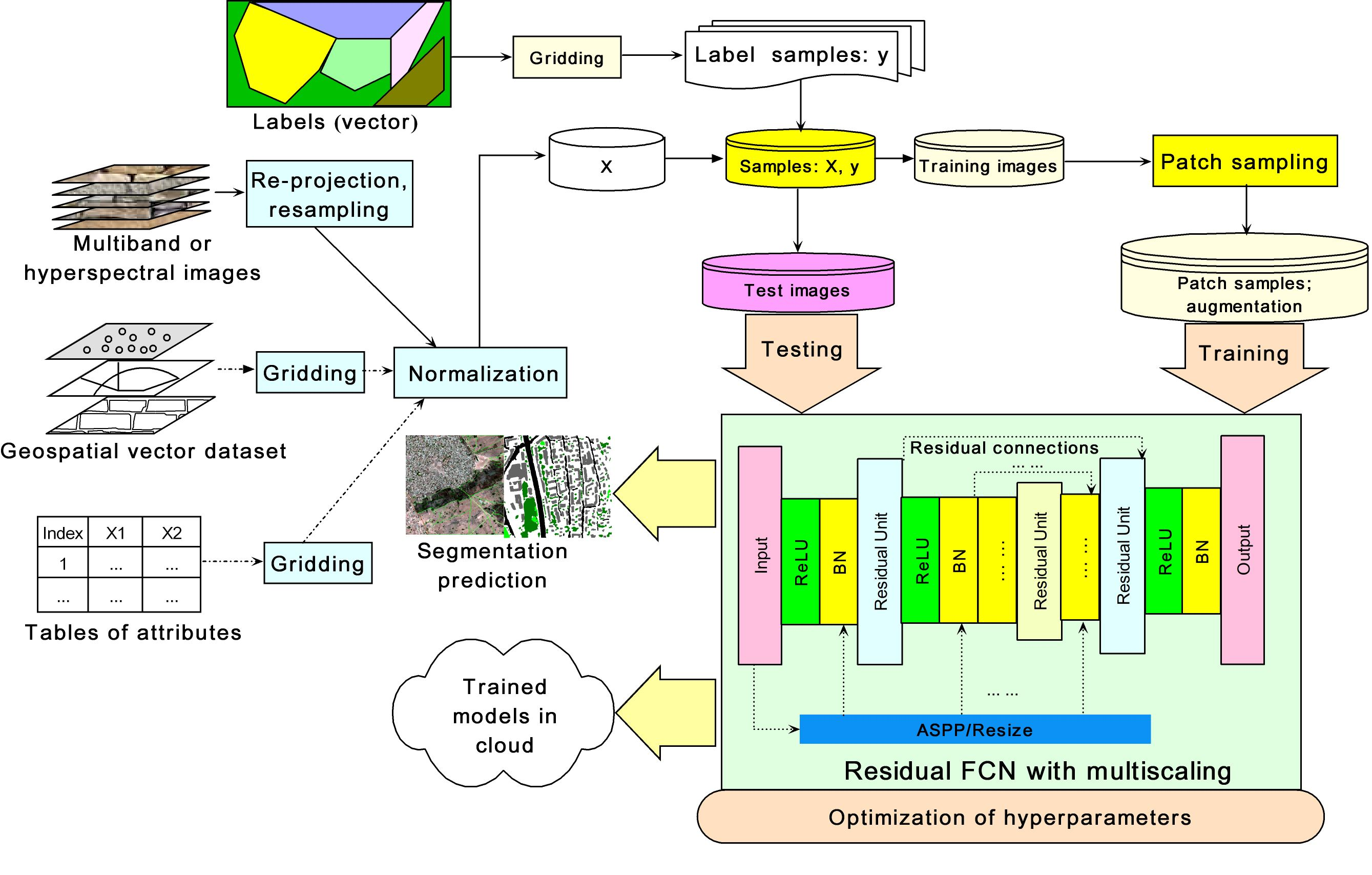
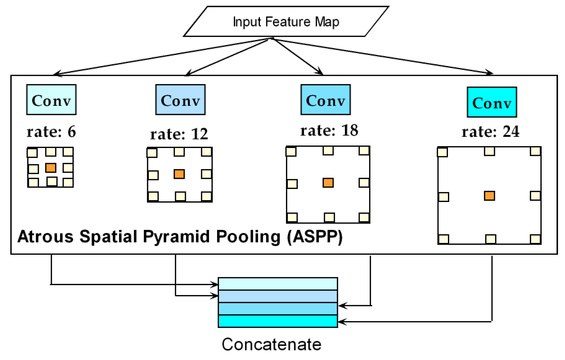
A traditional residual CNN consists of many residual units. Figure 1 shows a typical residual unit (a) and multiple stacked residual units (b) in a residual CNN. Here, the identity mapping shortcuts are implemented in the form of a continuously stacked sequence to establish residual connections and consequently enable the backpropagation of errors in learning, very similar to ensembles of relatively shallow networks [46]. Residual learning has effectively improved learning and model performance in many applications, including but not limited to classification [36,37], image superresolution [47], image compression [48], semantic segmentation [30,49], video understanding [50], the action segmentation of videos [51], and the spatiotemporal estimation of citywide crowd flows [52], vehicle flows [53] and influenza trends [54].
Except for a few studies, including that of Tran et al. (2017) [55], who used cascaded simple residual autoencoders for residual learning, most existing studies of residual CNNs have been based on the residual unit structure (Figure 1) presented by He et al. (2016) [36]. These residual units effectively mitigate the issues of saturation and degradation of accuracy with an increasing number of hidden layers and improve model performance, as demonstrated in many applications.
2.2. Multiscaling and ASPP
Multiscaling refers to variation in scale (resolution) in the image input due to different spatial, temporal, or/and measurement contexts. A CNN has an architecture that consists of multiple convolutional layers of a fixed resolution and size. These convolutional layers (filters) implicitly learn to detect features at a prespecified scale with an assumed degree of invariance. Consequently, the resulting models might be difficult to generalize to different scales [11]. The introduction of multiscale CNNs can result in trained models that can better adapt to scale variations in the input than single-scale CNNs, and can generate robust predictions for images at different scales. Raj et al. [56] designed two CNNs of different scales, one with shallow convolution and the other with a fully convolutional VGG (Visual Geometry Group)-16 architecture, and merged their predictions to generate a single output. Roy et al. [57] designed four multiscale CNNs with the same architecture used by Eigen et al. [58] and concatenated them in a sequential way to predict depths, normals and semantic segmentation labels. Bian et al. [59] designed n FCNs at different scales based on a two-stage learning approach, with the advantage of the ability to efficiently add newly trained models.
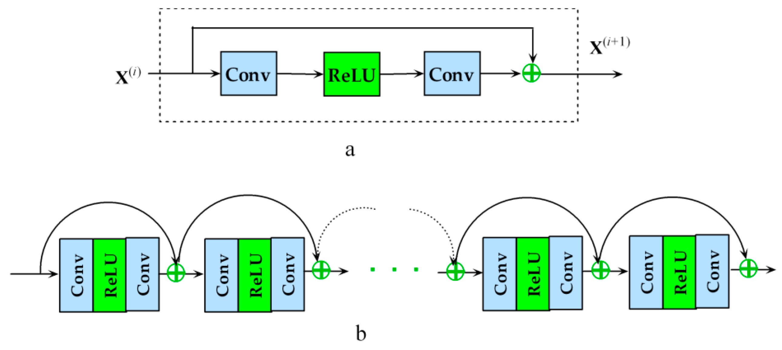
Recently, based on an autoencoder with an encoder-decoder structure (called Micro-Net), Raza et al. [60] resized the inputs to different scales corresponding to different encoding layers and concatenated the resized layers to improve the performance. In addition, dilated convolutions, also called atrous convolutions, which are derived from Kronecker-factor convolutional filters [61], leverage upsampling (controlled by the atrous rate) to exponentially expand the receptive field with no loss of resolution. Thus, such convolutions actually act as feature filters for multiscale information. Chen et al. [20,24,62] designed ASPP to capture multiscale context information. In ASPP, multiple atrous (dilated) convolutions at different atrous rates (r) are used to extract feature representations in a multiscale context (Figure 2) and are concatenated with other layers to improve the robustness of the trained models to variations in scale.
2.3. Semantic Segmentation via Deep Learning
In previous decades, methods of pixelwise classification based on hand-engineered features were the mainstream approaches for semantic segmentation, and classical machine learning methods such as mutual boosting [63], random forests [64] and support vector machines [65] were used. In addition, plain [66], higher-order [67] and dense [68] CRFs were developed as context models to capture complex relationships among interconnected pixels. Then, a CNN could be used as an image-patch classifier to capture the neighborhood context [69,70]. However, these methods are highly demanding in terms of computing resources and do not consider information from a sufficiently wide context for semantic segmentation [12].
In recent years, FCNs [16] have driven considerable advances in semantic segmentation in terms of learning efficiency and performance [12]. Based on the FCN architecture, upsampling (e.g., bilinear interpolation) was introduced (called UP_FCN) to obtain high-resolution images from the coarse-resolution predictions, and end-to-end training was conducted for the high-resolution output [71]. Dilated convolutions were also proposed to achieve finer resolutions without the introduction of additional parameters [19,22]. Furthermore, skip connections were leveraged to help UP_FCN or similar models to capture low-level visual information that could not otherwise be captured. Typical examples of networks with skip connections include FCNs [16], U-Net [72] and GCNs [23]. Many authors have also considered the incorporation of CRFs into the UP_FCN architecture, i.e., the incorporation of a priori domain knowledge to improve the robustness of the trained models. For example, Chan et al. [19] used mean-field inference to obtain a sharp boundary based on a dense CRF, and Zheng et al. [73] unified a CNN with CRFs by means of a recurrent neural network (RNN) to simulate CRF iterations within an end-to-end training procedure. Arnab et al. [74] further derived CRFs with higher-order potentials, thus achieving significant improvements over the CRF_RNN architecture. In addition, residual learning has been used in a limited way in CNNs for semantic segmentation [30,49] based on given differences between the encoding and decoding layers. Multiscaling in the UP_FCN architecture is also emerging as a means of enhancing the trained models’ robustness to scale variations [19,56,57,59,60], as previously mentioned.
However, although many advanced techniques have been proposed and corresponding models have been developed to achieve cutting-edge performance, many of these models (e.g., DeepLab [19,20,24,62]) are based on feature representations extracted using extensively pretrained models (as the encoding part of such a model), such as AlexNet [75], VGG-16 [76], GoogLeNet [77], or ResNet [36]. These pretrained models are often based on general or natural scene images consisting of RGB or RGB-D channels and thus are not designed for remotely sensed images, as aforementioned. Consequently, they cannot be directly used for the semantic segmentation of remotely sensed images. Therefore, to allow these advanced techniques (e.g., residual learning and multiscaling) to be effectively leveraged for the semantic segmentation of remotely sensed images, it is important to consider both suitably flexible UP_FCN architecture of deep learning and sufficiently qualified training samples of RS images.
3. Deep Residual Autoencoder with Multiscaling
This section presents the proposed flexible autoencoder-based architecture (Section 3.1) for the semantic segmentation of remotely sensed images, which extensively leverages residual learning (Section 3.2) to improve the learning efficiency and takes advantage of the multiscaling (Section 3.3) of the input images/features to make the trained model robust to scale variations. The implementation and evaluation of the proposed architecture are described in Section 3.4 and Section 3.5.
3.1. Autoencoder-Based Architecture
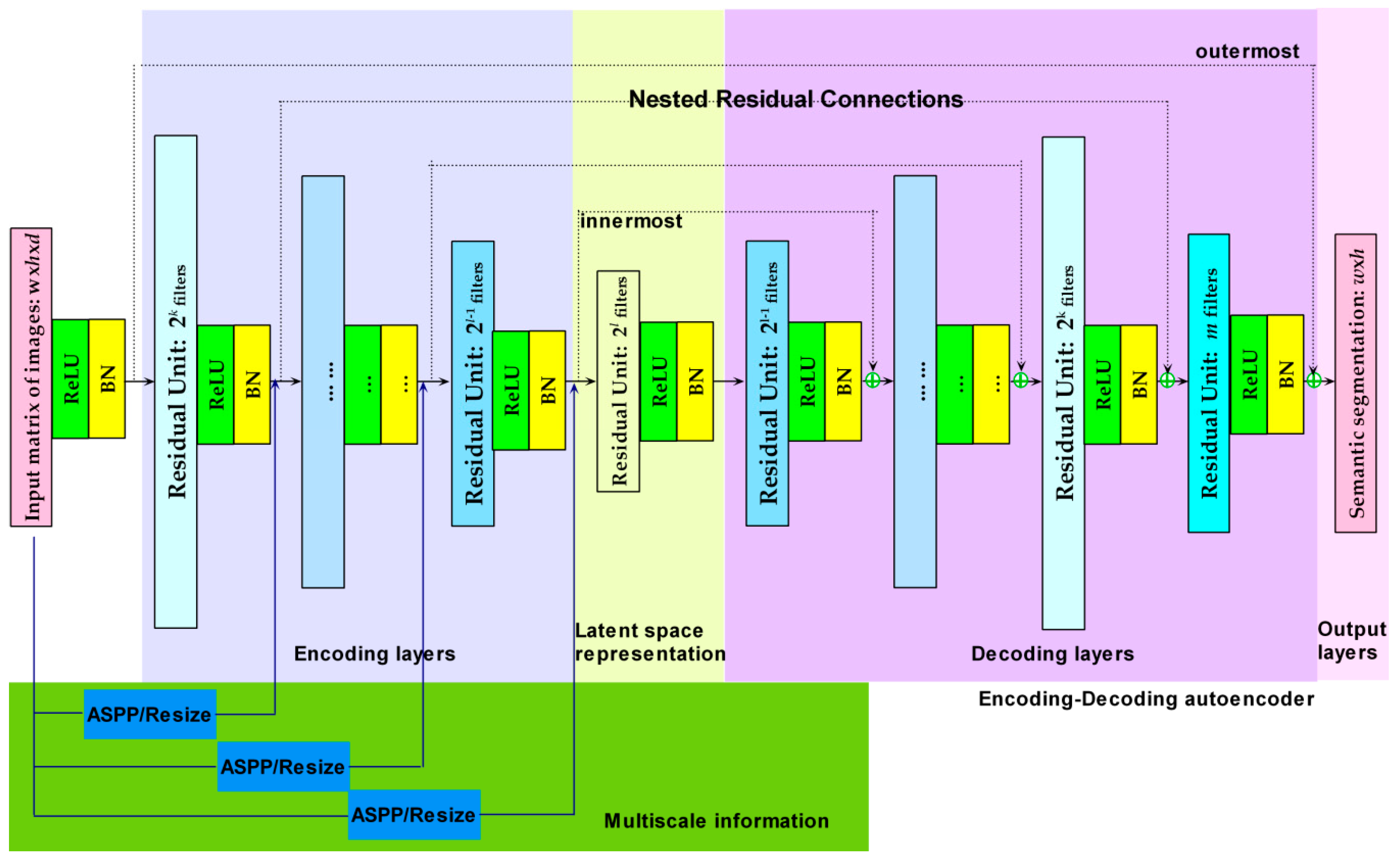
The presented architecture (Figure 3) is based on an autoencoder with residual connections and multiscaling via ASPP or resizing. In this architecture, the rectified linear unit (ReLU) activation function and batch normalization (BN) are mainly used in the hidden layers, as shown.
As a type of neural network, an autoencoder aims to learn an efficient data coding scheme or representation for a set of data [78,79], typically with the objective of dimensionality reduction, in either a supervised or an unsupervised manner. Through learning, an autoencoder can filter out signal “noise” and encode a representation that is as close as possible to the original input. Informative latent representations extracted by an autoencoder can effectively improve classification and semantic segmentation performance [80]. Notably, an autoencoder has a symmetrical structure, with the encoding layers and the corresponding decoding layers having the same numbers of nodes or the same dimensions, thus satisfying the requirement for nested residual connections.
3.2. Two Types of Residual Connections
An autoencoder-based architecture with nested residual connections was first proposed for an MLP in the author’s previous work [39]. Such deep residual MLPs show better learning efficiency and performance than regular MLPs do in practical applications [38,39,81]. Here, the concept of nested residual connections is generalized to an FCN for semantic segmentation. Unlike the residual units (Figure 1) in a traditional residual CNN, the nested residual connections realize identity mapping from each encoding layer to its corresponding symmetrical decoding layer (Figure 3). Therefore, all the residual connections are organized in a nested way from the outermost connection to the innermost connection, as shown in Figure 3. In addition to the nested residual connections, traditional residual units [36] are also incorporated within each encoding or decoding layer to boost the efficiency of residual learning to the greatest possible extent, as shown in Figure 3.
Residual connections require that both layers to be connected have the same number of nodes (for an MLP) or the same feature map dimensions (for a CNN). Consider a decoding layer l and its corresponding decoding layer L; xl and yl denote the input and output, respectively, for layer l, and xL and yL denote the input and output, respectively, for layer L. Here, the concept of identity mapping is used to establish residual connections. Thus, we have the following formula for the output of layer, L to illustrate the back-propagation of the errors in a residual connection:
where fl(xl,Wl) and fL(xL,WL) are the activation functions for the shallow layer l and the corresponding deep layer L, respectively, and where represents the recursive function of the shallow layer’s input, xl for the deep layer’s input, xL.
Suppose that L is the loss function. Based on automatic differentiation [82], we obtain the derivative of the loss function with respect to the input to layer l as follows:
According to Equation (2), introducing a residual connection () for identity mapping from a shallow layer (l) to the output of its corresponding deep layer (L) results in one constant term of 1 in the derivative of the output ( to ). If a linear activation function is applied to (i.e., ), then Equation (2) can be further simplified.
Based on Equation (2), the constant term 1 can allow the error information of (or if a linear activation function is used as ) to be directly backpropagated to the shallow layer without the need for any weight layer. Since is not always equal to -1 to cancel out the gradient for minibatch learning, this can effectively reduce the vanishing of gradients in the backpropagation of signal errors and hence mitigate the accuracy degradation during learning [39]. If an activation function with fully or partially linear feature mapping, such as a linear function, the ReLU function or the exponential linear unit (ELU) function, is used as , then the simplified derivative of the loss function can ensure the efficient backpropagation of the error information.
Although residual learning must always be based on a similar principle to that shown in Equation (2), residual connections can be implemented in two different ways, i.e., in traditional residual units or in a nested way. Figure 1 shows a typical residual unit consisting of two convolutional layers and one ReLU layer, possibly with the addition of a BN layer. In such a residual unit, the output of the first convolutional layer needs to have the same dimensional size and number of feature maps as the output of the last convolutional layer. Thus, residual connections are implemented within a residual unit. Since every layer in an autoencoder usually differs from its sibling and parent layers in terms of its dimensional size and number of feature maps, the error information cannot be directly recursively backpropagated. By contrast, the proposed residual connections [39] between the encoding and decoding layers enable the direct backpropagation of the errors to the shallower layers in a nested way (Figure 3).
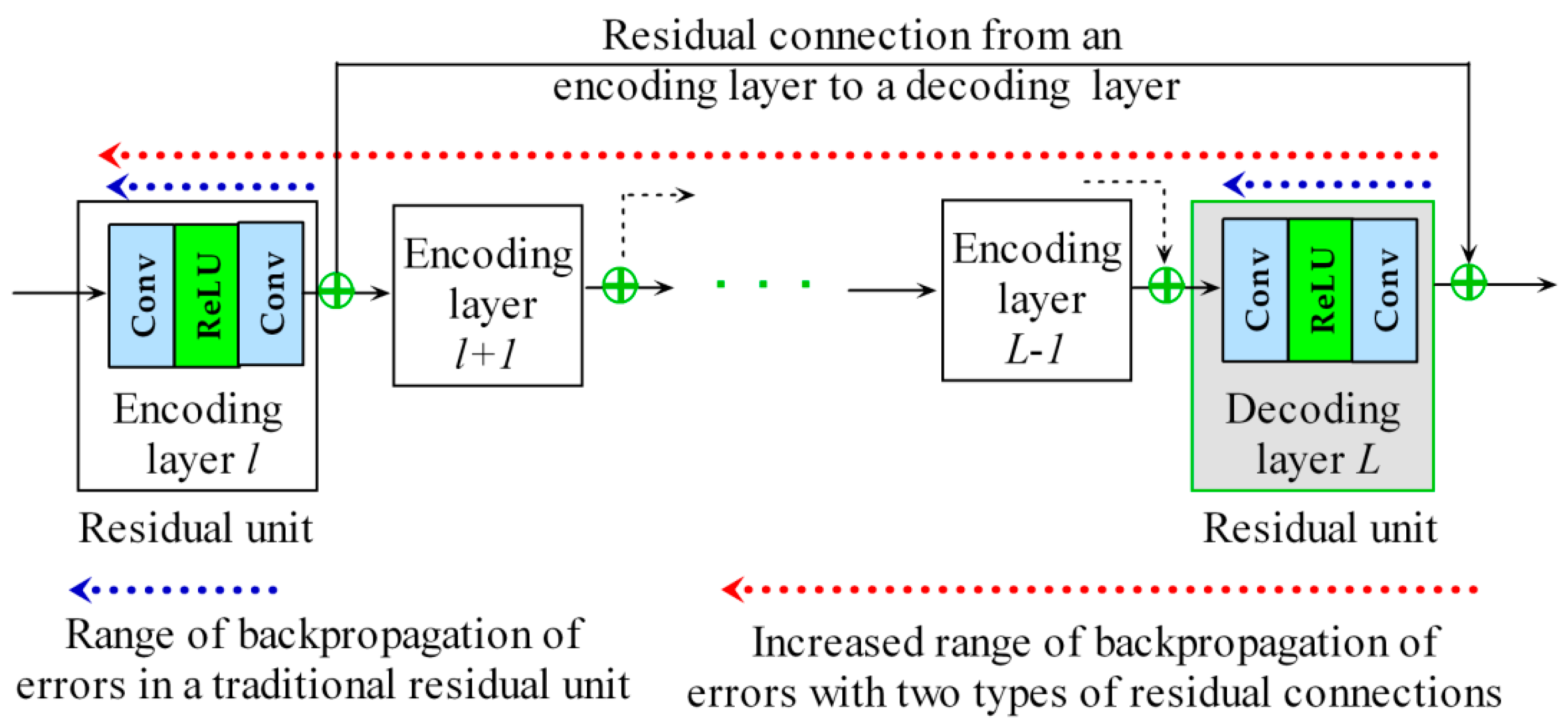
Compared with the UP-FCN-based U-Net architecture [72], which uses skip connections from the shallow encoding layers to capture low-resolution information via concatenation, the presented approach uses residual connections to capture such information with fewer trainable parameters. Since the introduction of residual connections does not increase the number of parameters and can improve the learning efficiency, in addition to the nested residual connections, residual units are also used in every encoding or decoding layer (thus, two or more convolutions with activation/ batch normalization are used within each encoding/decoding layer) to improve residual learning to the greatest possible extent. Using both types of residual connections can more efficiently boost the backpropagation of errors and subsequent learning compared with residual units alone [30] since the introduction of a residual connection from an encoding layer to its corresponding decoding layer considerably lengthens the path of the total residual connection, thus extending the range of backpropagation, as indicated by the red dotted line in Figure 4.
3.3. Incorporation of Atrous Convolutions and Multiscaling
Studies show that incorporating multiscale information can improve a trained model’s ability to handle both local and large objects [83] and its robustness to scale variations [11], as mentioned above. Thus, in the presented architecture, multiscale information is extracted from the input images and fused via ASPP or resizing (Figure 3).
ASPP (Figure 2) is derived from the DeepLab model of Chen et al. [20]. In ASPP, multiple parallel atrous convolutional layers at different sampling rates (atrous rates) are used to capture local information at multiple resolutions (scales) and are then concatenated into a target convolutional layer. In the presented architecture, multiple atrous convolutions are used to multiscale the input images via ASPP to be fed to the intermediate encoding layers (via concatenation) at different scales. ASPP involves additional atrous layers with trainable parameters that may require a massive amount of memory space, beyond what is practically available. Consequently, the numbers of atrous layers and feature maps in ASPP may be limited by the available computing resources.
As an alternative approach, resizing to different resolutions has also been used to multiscale input images to achieve improved performance in the semantic segmentation of medical images [60]. Compared with ASPP, this method is relatively simple and easy to implement. Thus, this method can also be used in the proposed architecture (Figure 3) as an alternative to ASPP if memory limitations prevent the optimal configuration of the atrous layers in ASPP.
3.4. Sampling of the Training Set and Boundary Effects
A high-resolution remotely sensed image usually cannot be stored in the memory space available for training. Therefore, the patch sampling method (Figure 5a) was used to obtain training samples of a small image size [72,84]. For binary semantic segmentation, oversampling and undersampling can be used for positive and negative instances, respectively. A small sliding window with a suitable sampling distance can be used to sample a large image to obtain patch samples. Oversampling can be applied for a small number of instances to increase the number of training patch samples; undersampling can be applied for a large number of instances to decrease the number of patch samples to maintain the balance in the number of training samples between the majority and minority classes. In terms of implementation, for oversampling, a short sampling distance can be used to obtain the patch samples with a proportion of overlapping areas; for undersampling, a long sampling distance can be used to obtain the patch samples with no overlapping areas but with a long distance between them. For multiclass semantic segmentation, oversampling or undersampling can also be used to obtain a suitable number of samples for training, depending on sample availability.
3.5. Metrics and Loss Functions
To evaluate the trained model’s performance, the following metrics were used:
(1) The pixel accuracy (PA) is a basic metric computed as the ratio of the number of correctly classified pixels to the total number of pixels.
where k is the number of classes and pij denotes the number of pixels of class i predicted to belong to class j. Usually, pii represents the number of the true positives, whereas pij and pji represent the numbers of false positives and false negatives, respectively.
(2) The Jaccard index (JI) is defined as the size of the intersection of two sets divided by the size of their union [69]. A well-known statistic for measuring the similarity of two sets, it is also called the intersection over union (IU or IOU) [16].
where c is the target class (c=1,2,…,k), P denotes the set of predicted pixels, and G denotes the set of ground-truth pixels.
(3) The mean intersection over union (MIoU) is computed by the JI on a per-class basis and then averaging over all classes.
Although the JI or MIoU is an important metric for evaluating the results of semantic segmentation, these metrics are not differentiable and thus cannot be used in the loss function for gradient descent optimization. However, the normal JI can be expressed in a differentiable form for optimization in gradient descent:
where denotes the normalized Jaccard index, denotes the ground-truth mask ( is the ground truth for the ith pixel), represents the predicted probability of belonging to the positive class ( is the predicted probability for the ith pixel), and ε is a small positive value that is used as a smoothing factor to avoid overflow due to a possible denominator of 0.
For binary semantic segmentation, the following binary cross-entropy loss is used with the normal JI:
Then, the total loss function for binary semantic segmentation can be defined as follows:
For multiclass semantic segmentation, the following multiclass cross-entropy loss can be used:
where denotes the ground truth for whether the ith instance belongs to class j and represents the predicted probability of the ith instance belonging to class j as obtained with the softmax function. Equation (10) refers to the softmax calculation of the probability, with denoting the output of the last layer before the softmax calculation.
3.6. Implementation
Regarding the core algorithm (deep residual autoencoder with multiscaling), a Keras version of the proposed method has been developed with TensorFlow as the backend. The package has been published as a Python package (https://pypi.org/project/resmcseg) and via GitHub (https://github.com/lspatial/resmcsegpub).
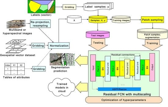
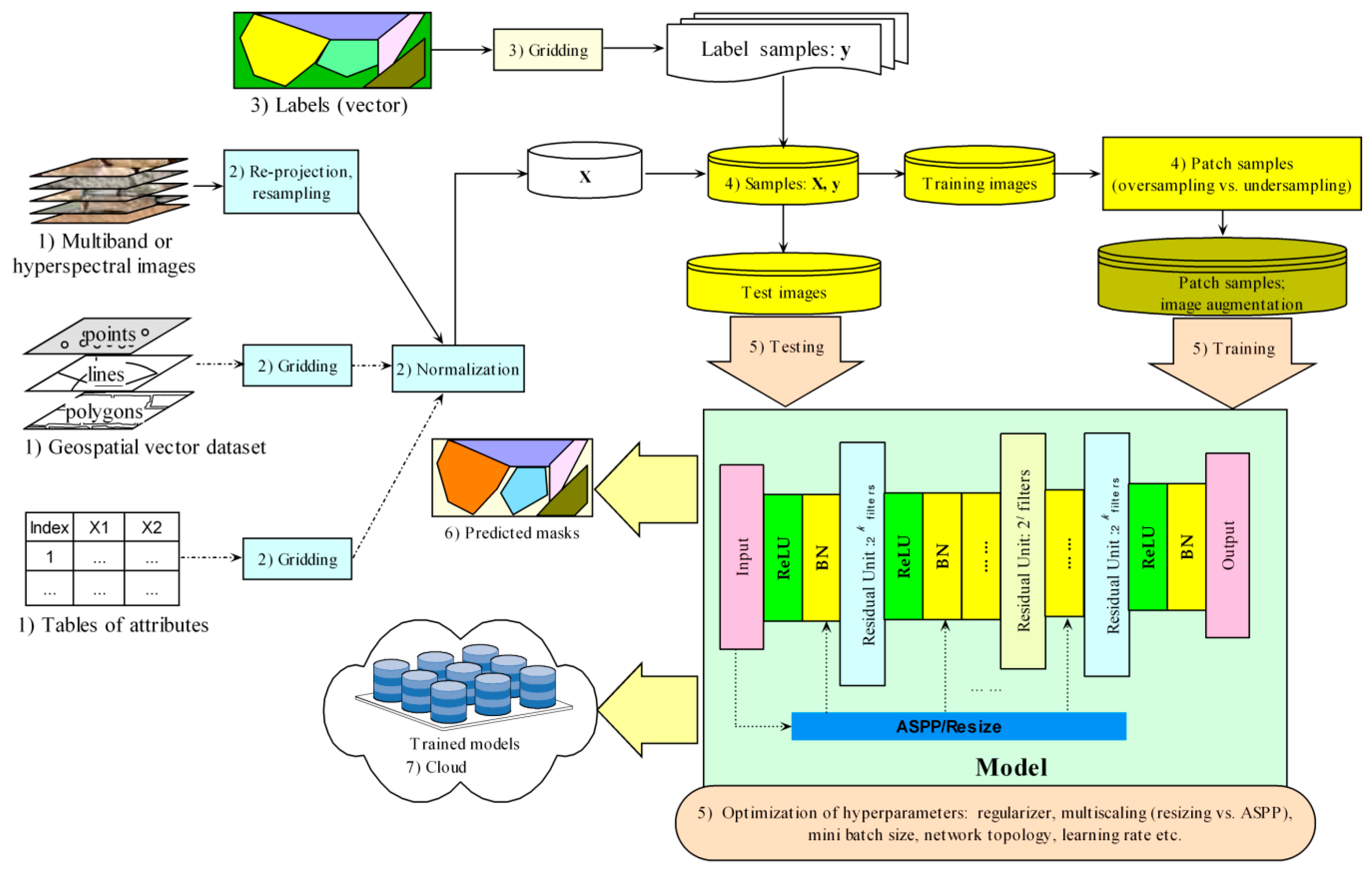
A workflow of implementation under geospatial context is represented in Figure 6. In this workflow, the predictors from geospatial dataset or/and the other attributes are also considered; re-projection and resampling used to processing geospatial dataset are also included. In total, seven steps are summarized for this workflow graph.
(1) Input predictors (X): besides the multiband or/and hyperspectral images, potential data sources from other geographical information science (GIS) (e.g., vector data of points, lines and polygons) and attributes database are also considered although not used in the test cases (thus presented in the dash-dot lines in this graph). These data may help improve semantic segmentation and thus is contained in the workflow.
(2) Preprocessing of the input predictors: preprocessing involves re-projection, resampling of the images at different spatial resolutions using bilinear interpolation to obtain the samples at a consistent target resolution and coordinate system, gridding of vector data, and normalization. For re-projection, resampling and gridding, the raster library (https://cran.r-project.org/web/packages/raster) of the R software provides the relevant functionalities. Normalization aims to remove the difference in the value scale between different predictors to improve learning efficiency. The Python’s scikit package (https://scikit-learn.org) provides a convenient normalization function.
(3) Input labels (y): the label data are essential for training of the models. Usually, the label data of vector format (points, lines or polygons) are obtained manually and must be gridded into the masks at the target resolution. A summary for the proportion of pixels for each label class can be conducted in this step.
(4) Merging of the data, sampling and image augmentation: this involves merging of the predictor and label data (X and y), random split of the training and test samples, patch sampling for the training samples by oversampling or undersampling, and image augmentation. As aforementioned in Section 3.4, patch sampling is to divide a large image into small patches for the purpose of training, and the summary of the pixel proportion for each class can be used to determine a strategy of patch sampling. Then, the training set (both images and masks) was randomly augmented at training time with rotations by 45 degrees, 15–25% zooms/translations, shears, and vertical and horizontal flips.
(5) Training and testing: this involves construction, training and testing of the models and grid search to obtain optimal hyperparameters (e.g., regularizer, network topology, multiscaling choice, mini batch size, and learning rate). The published Python package of core algorithm, resmcseg, can be used to construct the proposed model with flexibility of different choices of hyperparameters. With different hyperparameters and their combinations, grid search [85] can be conducted to find an optimal solution for these hyperparameters.
(6) Prediction: this involves use of the trained models to predict the land-use mask of the new dataset. In addition, the predicted mask can be converted into the output of vector format for use under geospatial context.
(7) Pre-trained models in cloud: the trained models can be stored as the pre-trained models in the cloud platform (e.g., Amazon Web Services or Google Cloud), and can be called later for predicting or as the basic models for further training.
4. Experimental Datasets and Evaluation
This section briefly describes the two experimental datasets (Section 4.1) involved in the test, and the evaluation of the proposed approach (Section 4.2).
4.1. Two Datasets
The presented methods were tested on two datasets.
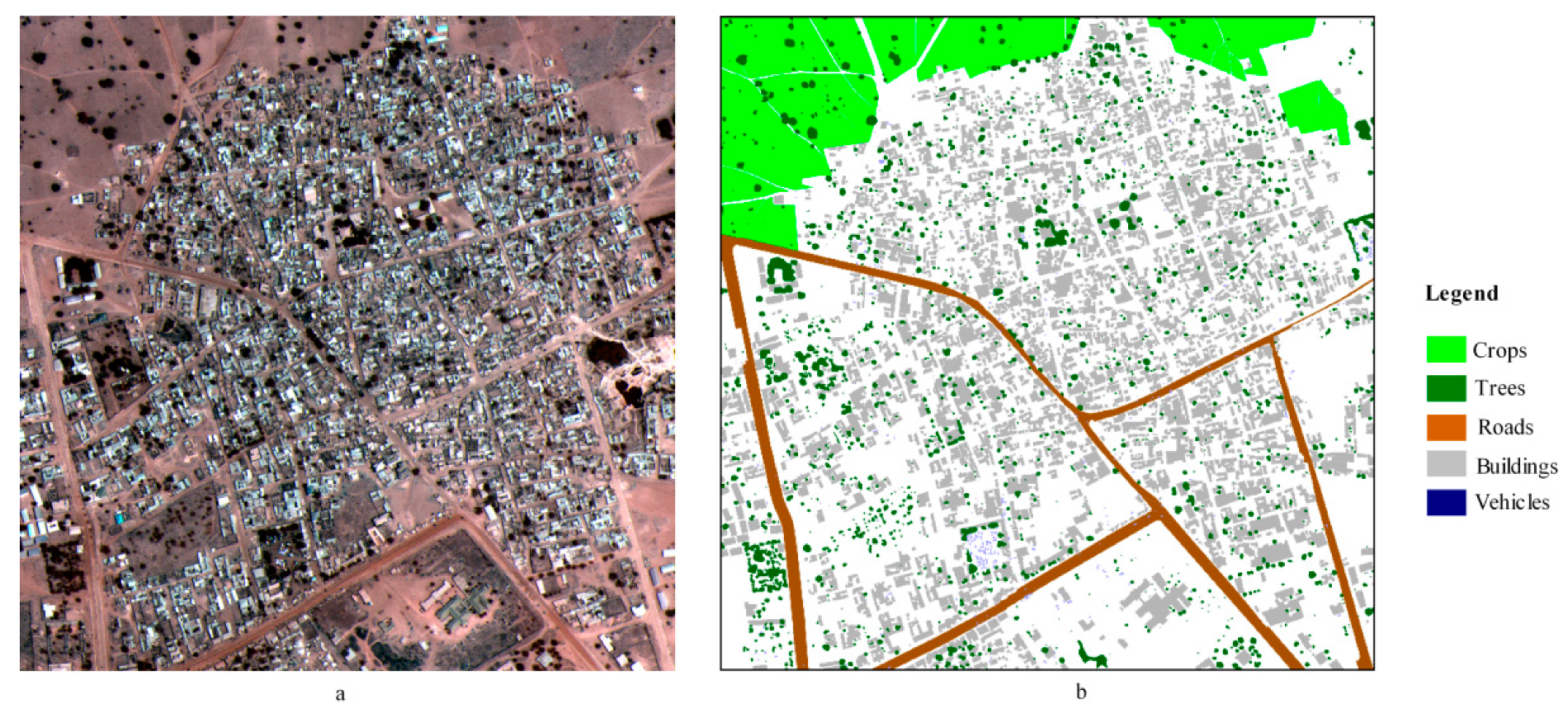
(1) The dataset from the Defense Science and Technology Laboratory (DSTL) Satellite Imagery Feature Detection challenge (https://www.kaggle.com/c/dstl-satellite-imagery-feature-detection) run by Kaggle in 2017 [40]. In total, 25 satellite images were used for training, validation and testing in this study. Each image covers 1 square kilometer of the Earth’s surface, and the images include different channel information: the dataset includes high-resolution panchromatic images with a 31 cm resolution, 8-band (M-band) images with a 1.24 m resolution, and shortwave infrared (A-band) images with a 7.5 m resolution. These images were obtained by the WorldView-3 satellite. Panchromatic sharpening [86] was used to fuse each high-resolution panchromatic image with the corresponding lower-resolution M-band and A-band images to obtain images with a 31 cm resolution. The task was to predict a class label for each pixel of the input image. Due to the imbalanced class distributions, much better results could be obtained by training a separate model for each class rather than a single model for all classes [84]. Thus, for this dataset, binary semantic segmentation was conducted separately for each of five classes, i.e., buildings, crops, roads, trees and vehicles. Figure 7a presents one of the DSTL images with its ground-truth mask (Figure 7b). Correspondingly, a comprehensive loss function, as seen in Equation (8), combining the normal JI and a binary cross-entropy loss was used.
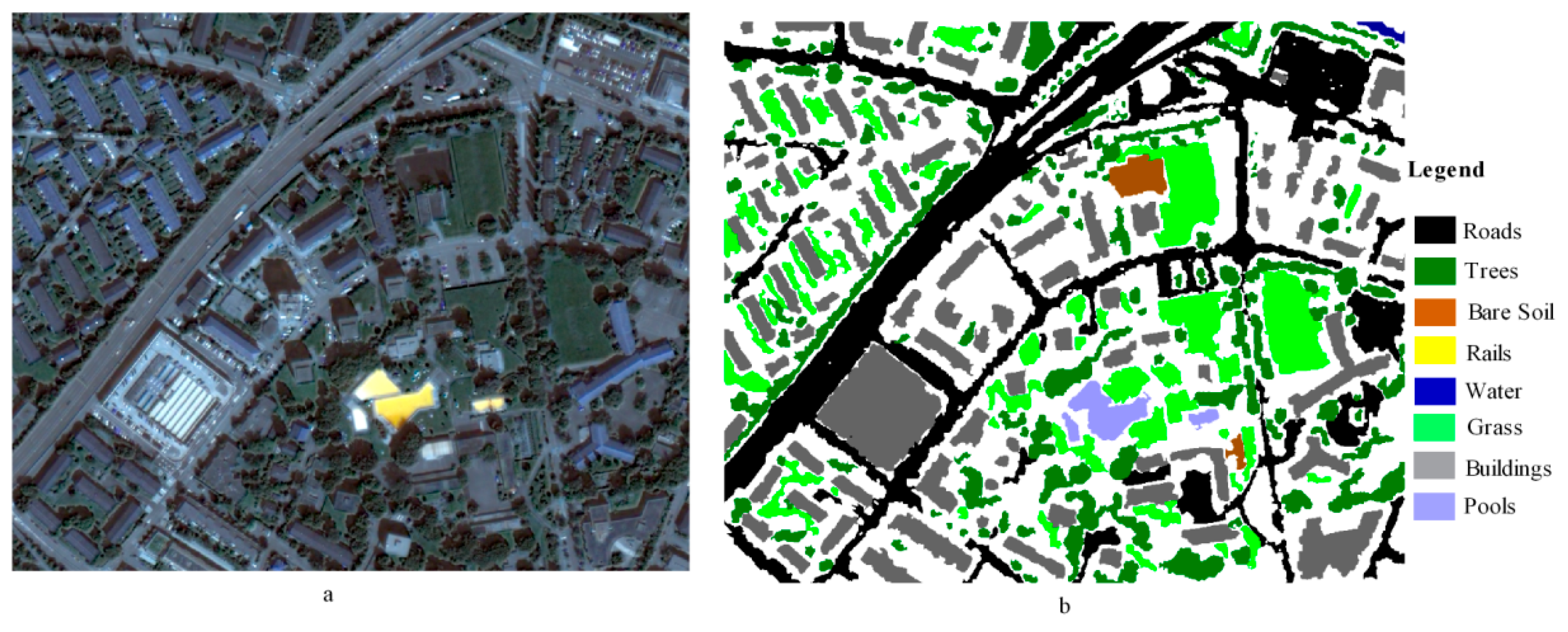
(2) A set of 20 multispectral very-high-resolution images acquired over the city of Zurich (Switzerland) (https://sites.google.com/site/michelevolpiresearch/data/zurich-dataset) by the QuickBird satellite in 2002 [41]. The average image size is 1000x1150 pixels, with 4 channels spanning the near-infrared to visual spectrum (NIR-R-G-B). The images after panchromatic sharpening have a 0.61 m spatial resolution. Ground-truth masks with 9 classes are provided for these images: road, trees, bare soil, rail, buildings, grass, water, pools and other (background). Figure 8a and b present one of the Zurich images and its ground-truth mask, respectively. For this dataset, the multiclass cross-entropy loss, as seen in Equation (9), was used to test the performance of the proposed method for multiclass semantic segmentation.
4.2. Training and Evaluation
For binary semantic segmentation (the DSTL dataset), oversampling for positive instances and undersampling for negative instances were conducted to obtain the patch samples (with an input patch size of 256x256, an output patch size of 224x224, and a border size of 16 on each side to eliminate boundary effects during segmentation). For a class with a small number of positive instances (e.g., vehicles), the oversampling distance can be a small value, with a large undersampling distance for negative instances, to obtain a sufficient and balanced number of training samples; for a class with many samples, the oversampling distance can be a large value, with a small undersampling distance for negative instances, to obtain balanced samples.
For multiclass semantic segmentation (the Zurich dataset), oversampling was conducted with a distance of 150 pixels to obtain a sufficient number of instances. The sizes of the input and output image patches were similar to those for the DSTL dataset.
The Adam optimizer with Nesterov momentum was used to train each model for 100 epochs with a learning rate that was initially set to 0.001 and was then adaptively adjusted during the learning process. An early stopping criterion was used. During training, each batch consisted of 15 image patches.
Four models, i.e., the benchmark U-Net, a residual autoencoder with no multiscaling, a residual autoencoder with resizing-based multiscaling, and a residual autoencoder with ASPP-based multiscaling, were trained and compared using the two datasets (DSTL and Zurich). To illustrate the generalizability of the proposed method, in addition to the tests in training, an additional independent test was conducted, i.e., no patch samples from the test images (10% of the total samples) were used to train the model, and the independent test results for three sample images from each dataset are presented.
5. Results
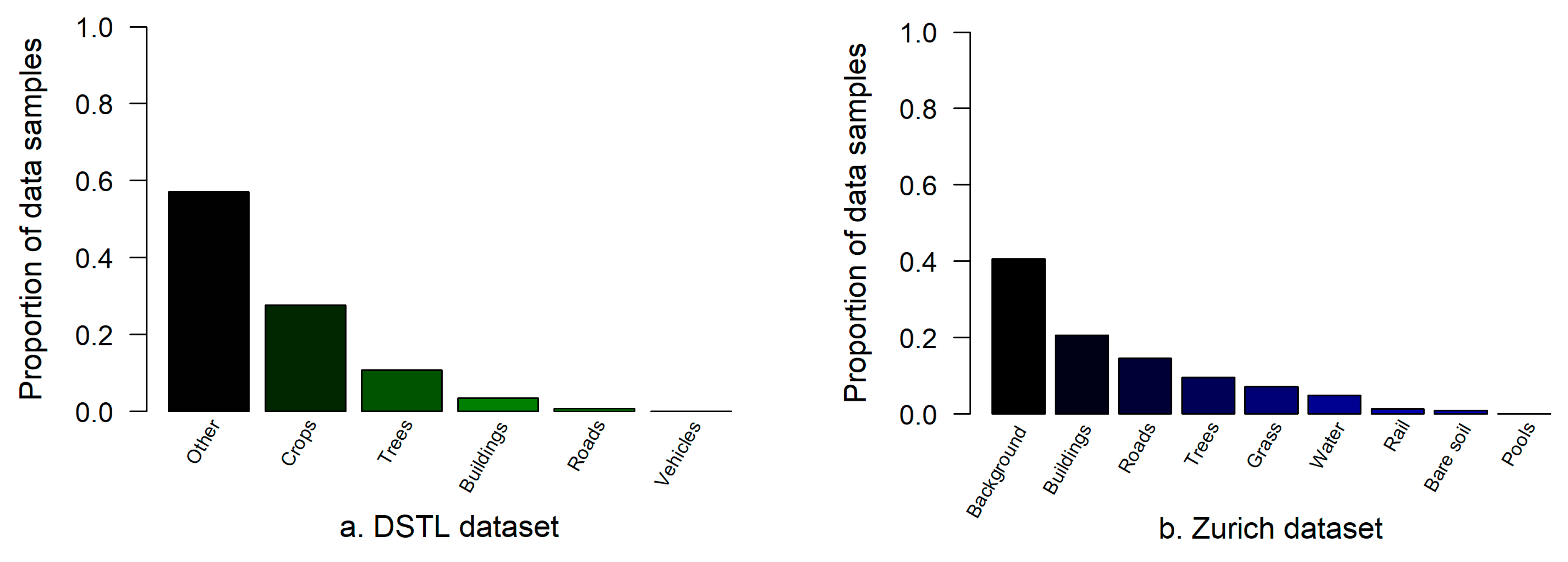
The proportional distributions of the different classes for the DSTL and Zurich datasets are represented in Figure 9a,b, respectively, and the corresponding sampling distances are summarized in Table 1. Using the parameters given in Table 1, each image from the two datasets was sampled to obtain the patch samples for training, validation and testing using a sliding window. Random splitting was applied to divide the patch samples as follows: 60% for training, 20% for validation and 20% for testing. The training set (both images and masks) was augmented at training time as mentioned in Section 3.6. No augmentation was performed on the validation or test data. Performance metrics for the training, validation and testing phases are reported.
The performances of the four models are presented in Table 2 (the statistical boxplots of JI/MIoU shown in Figure 10), and the learning curves in the training and validation phases are shown in Figure 11 for the DSTL dataset and in Figure 12 for the Zurich dataset.
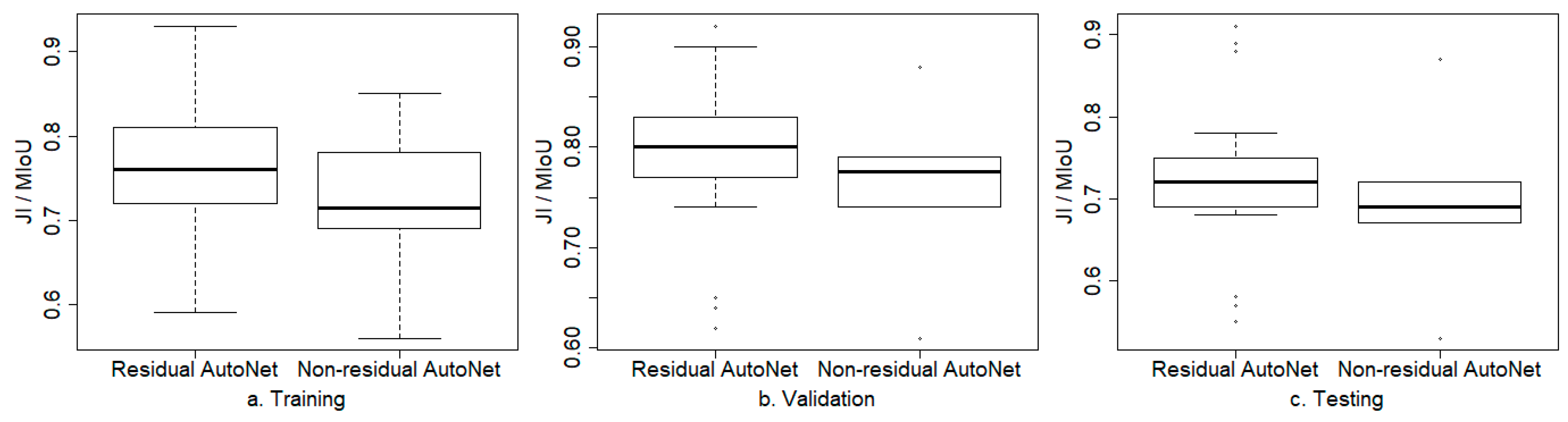
The results show that, compared with the baseline U-Net model, the PA of the presented residual autoencoder with no multiscaling was improved by 1–6% in the training phase (and by 1–5% in the validation and testing phases) except the classes of buildings and vehicles of the DSTL dataset, and the JI or MIoU was improved by 2–11% in the training phase (and by 1–8% in the validation phase and 1–9% in the testing phase). Thus, residual learning improved the JI or MIoU more than it did the accuracy. The statistics (Figure 10) show that residual autoencoders (with and without multiscaling) improved JI/MIoU averagely by about 4.1% over that of non-residual autoencoders in training (0.76 vs. 0.72), by about 2.7% in validation (0.79 vs. 0.76) and by about 2.9% in testing (0.72 vs. 0.69).
Multiscaling via ASPP was beneficial for the semantic segmentation of crops and buildings in the DSTL dataset (further improving the JI by 2–3% in validation and by 3% in testing relative to the results of the residual autoencoder with no multiscaling). However, multiscaling via ASPP did not improve the performance of the residual autoencoder for the semantic segmentation of trees, roads and vehicles in the DSTL dataset nor for the Zurich dataset. For the segmentation of trees, multiscaling via resizing very slightly improved the JI in the training, validation and testing compared with the results obtained with ASPP. Multiscaling via either resizing or ASPP did not always improve the performance of the residual autoencoder. As shown in Table 2, the residual autoencoder with no multiscaling achieved the best performance for the binary semantic segmentation of roads and vehicles in the DSTL dataset and for multiclass segmentation in the Zurich dataset. For these segmentation tasks, the JI or MIoU of the residual autoencoder was improved by 9-11% in training, 4-8% in validation, and 5-9% in testing compared with the performance of U-Net. The incorporation of multiscale information did not improve either the JI or the MIoU; in fact, both metrics decreased in value.
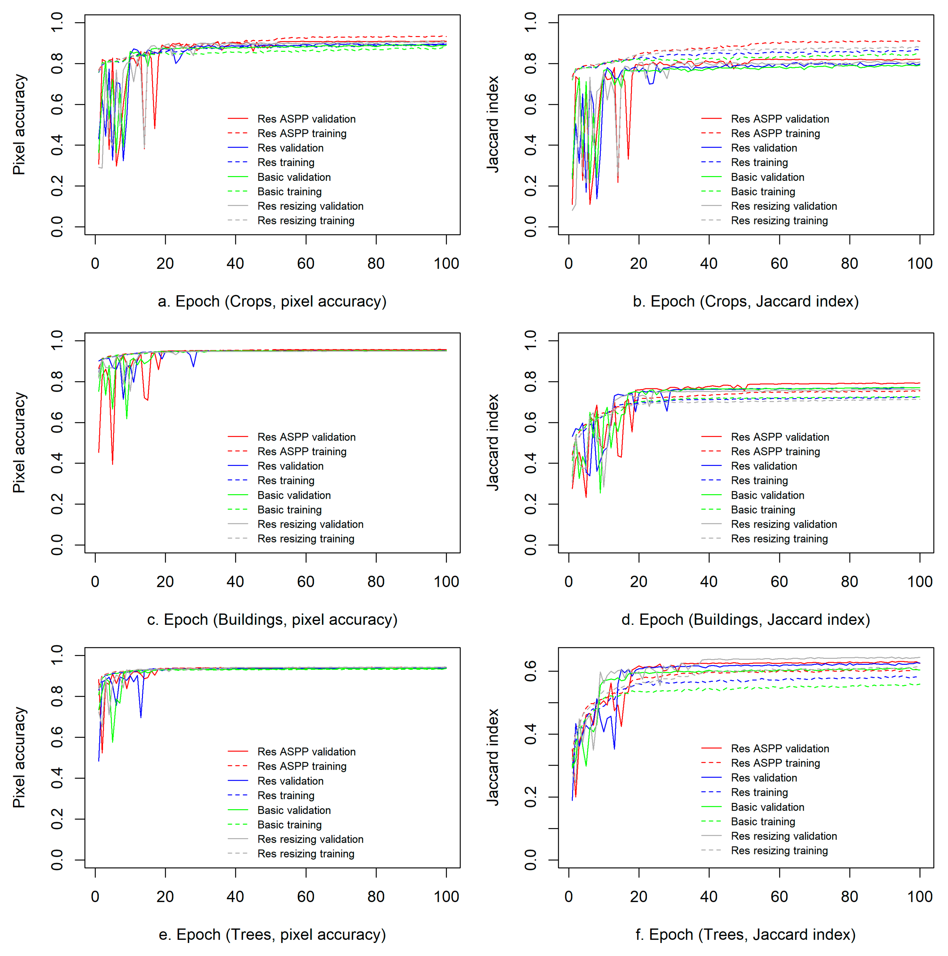
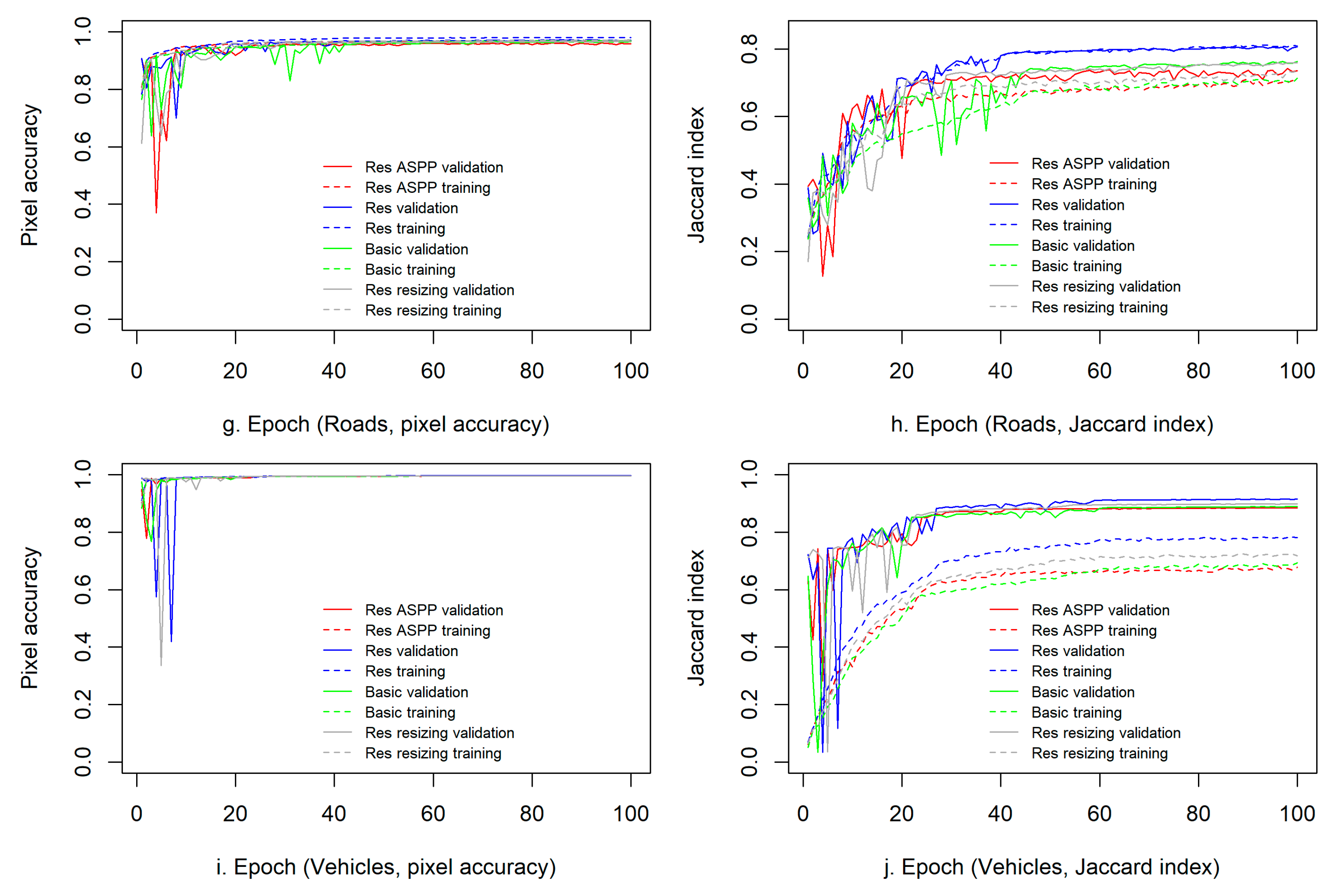
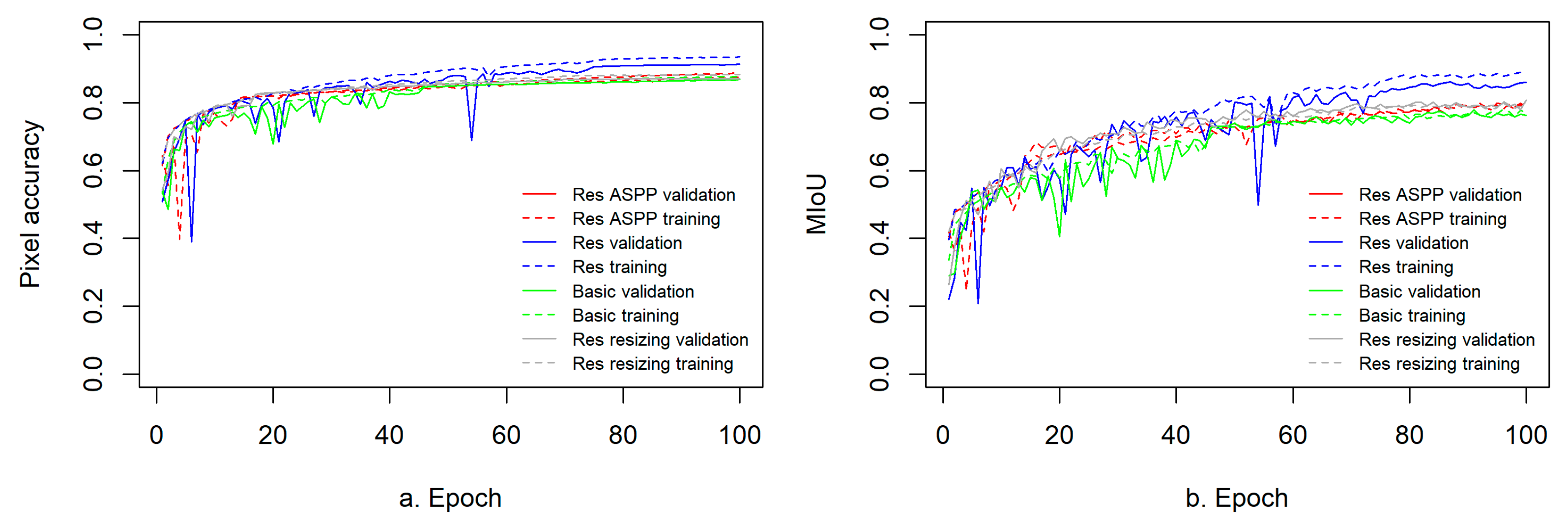
The learning curves for the PA and JI or MIoU metrics (Figure 11,Figure 12) also exhibit consistent trends of better performance for the deep residual autoencoder than for the baseline U-Net model for each binary segmentation task on the DSTL dataset and for multiclass segmentation on the Zurich dataset. For the road and vehicle (Figure 11h,j) classes in the DSTL dataset and for the multiclass Zurich dataset (Figure 12b), the learning curves for the JI or MIoU also shows higher values for the residual autoencoder with no multiscaling, than those for the other three models during the later phase of training.
As shown in Table 2, the residual autoencoder with no multiscaling has the fewest trainable parameters (approximately 28 million) among all considered models. A smaller number of model parameters may result in less overfitting.
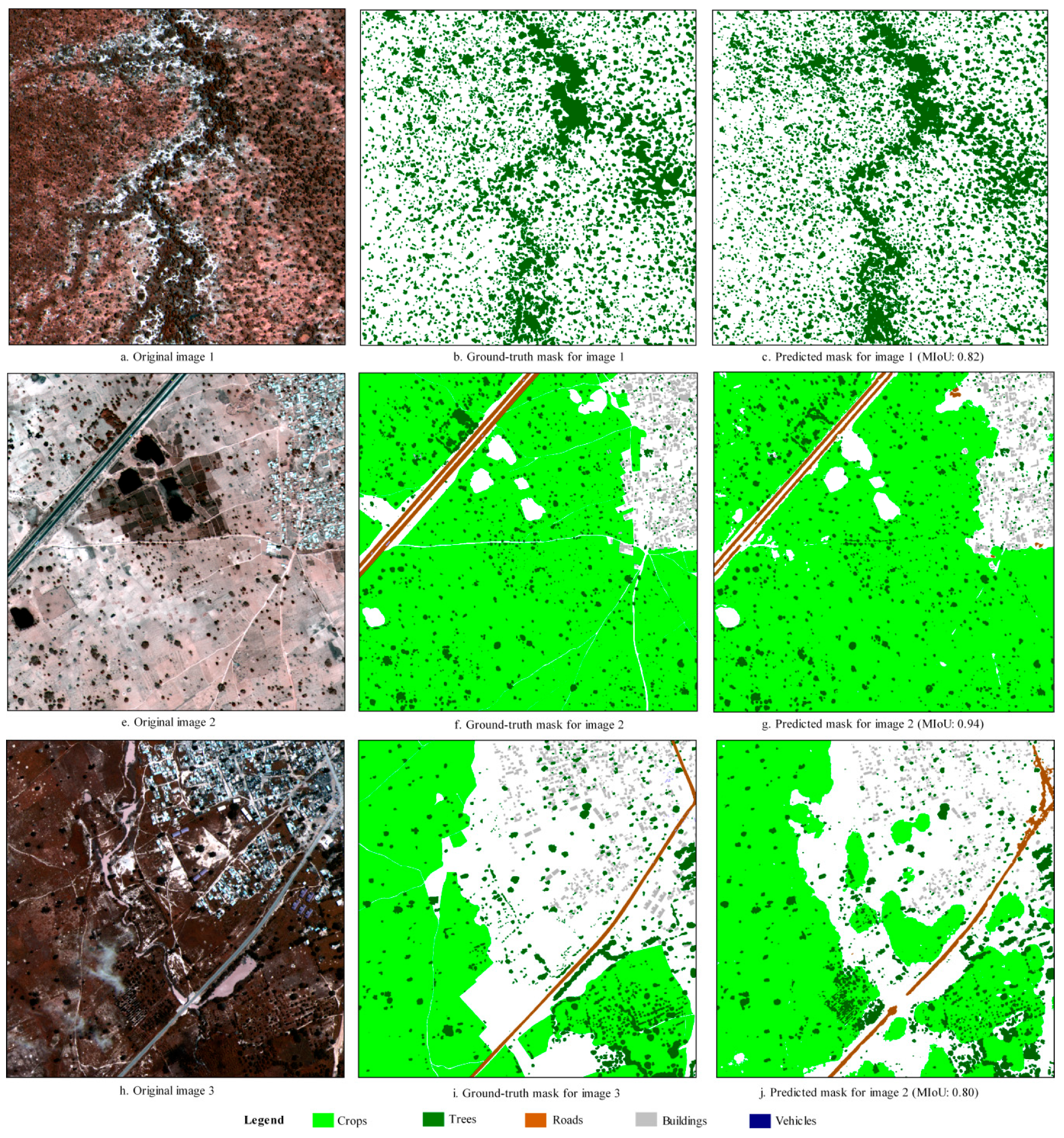
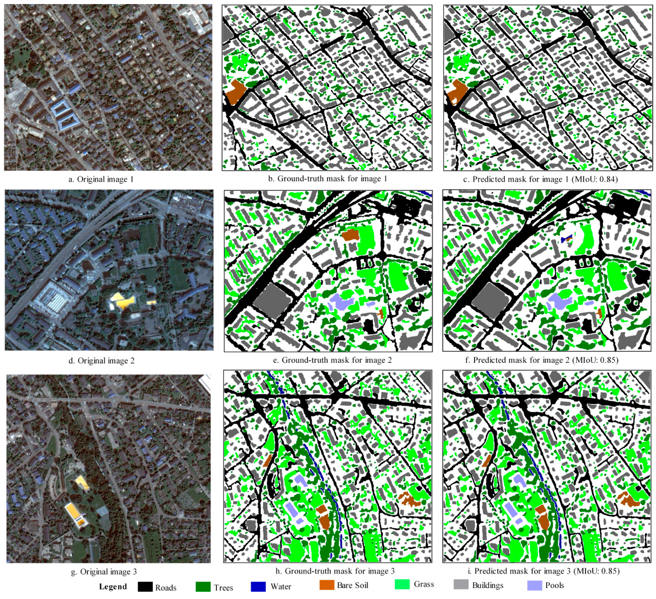
Figure 13 and Figure 14 each present three images: their ground-truth masks and the masks predicted in the independent test for the DSTL and Zurich datasets, respectively. As shown in these results, the proposed method captured the majority of the ground-truth masks for both binary (JI: 0.80-0.94) and multiclass (MIoU: 0.84-0.85) segmentation, illustrating its practical reliability. As demonstrated in these two experiments, the proposed method achieves a significant improvement over the benchmark method, U-Net.
6. Discussion
For limited applications of deep learning in semantic segmentation of remotely sensed images, this paper presents a flexible novel approach to leverage extensive residual connections within and between all encoding and decoding layers to improve learning efficiency and performance of the trained models. Given the variation in scale for many geospatial applications, the proposed approach also incorporates multiscaling via resizing or/and ASPP. For practical applications, multiple sources of data including geospatial data of vector format and/or attributes can be fused (Figure 6) if available. These auxiliary data may provide important background information as the constraints of a priori geoscience knowledge for the models, probably helping improve generalization and reduce over-fitting. Correspondingly, for geospatial data from multiple sources with different scales and data formats, re-projection, resampling and gridding may be needed as the preprocessing steps to obtain qualified training samples at a consistent target resolution and coordinate system. It must be admitted that these preprocessing steps may introduce the variation of the input. As shown in the results of the study cases, the variation just generated limited influence on training and prediction of the models. This illustrates applicability of deep learning for semantic segmentation of remotely sensed images with other potential geospatial data.
As shown in the results, the incorporation of multiscale information does not always improve the performance of the trained model. For a minority class (a class with a small number of positive instances, e.g., roads and vehicles in the DSTL dataset), the incorporation of multiscale information does not necessarily improve the model’s performance due to insufficient samples used in training to capture variation in scale, and more positive samples may be helpful for training the multiscale models. Inversely, for a majority class (a class with a large number of positive instances, e.g., crops and buildings in the DSTL dataset), the incorporation of multiscale information via resizing or ASPP might improve the model’s ability to capture local objects and its invariance to scale, as demonstrated by the segmentation of crops and buildings in the DSTL dataset.
In multiscaling via ASPP, atrous convolutions with increasing dilation rates are used to widen the receptive field. Multiscaling via ASPP can improve the network’s ability to capture local objects and its robustness to scale variations [18], as shown by the results for crops and buildings in the DSTL dataset. Traditional residual learning has previously been combined with atrous convolutions [49] to eliminate the “degridding” effects caused by the use of atrous convolutions. Due to the limited available computing resources, only 4 atrous convolutions (with dilation rates of 1, 4, 8, 16) were applied in parallel with a small number of filters in these experiments, and training was also limited by the small mini batch size (15). With more computing resources, more powerful tools such as vDNNs (virtualized deep neural networks) [87] and more available positive image samples, the training capabilities for multiscaling via ASPP may be enhanced to improve the robustness to scale variations.
The results show that extensive residual connections were effectively used in the autoencoder-based FCN architecture of deep learning to improve the performance, similar to that in deep residual MLP [38,39]. The sensitivity analysis also showed that the proposed extensive residual connections within and between all encoding and decoding layers achieved better performance than traditional residual connections alone for the DLST and Zurich datasets. Theoretically, as mentioned, extensive residual connections lengthen the path for direct backpropagation of errors, thus improving the trained model’s performance. Even without the use of multiscaling, a deep extensive residual FCN still achieved a considerable improvement over U-Net for semantic segmentation of RS images.
It must be admitted that the proposed extensive residual learning can also be applied for images of other types (e.g., natural scenes and medical images). However, for this study, the deep residual autoencoder architecture was specially developed and trained for semantic segmentation of remotely sensed land-use images. Two different datasets were used in the tests to illustrate the generalization of the proposed method for segmentation of RS images. Given the multiscale effect for RS and geoscience applications [88], the proposed method incorporated multiscale input for invariance to scale variations. Based on the flexible architecture and the author’s published python package, resmcseg (https://pypi.org/project/resmcseg) for this paper, the model can be easily adjusted in the network topology (e.g., number of hidden layers), multi-scaling, residual connections and output type etc. to achieve an optimal effect. The pretrained models for the two datasets have been stored in the cloud platform and shared through the publically available interface. For practical applications under geospatial context, the raster package of the R software provides reliable functionalities of re-projection, resampling and gridding; the python’s scikit provides the functionalities of normalization, random sampling and one hot encoding.
One limitation of the presented method is the lack of postprocessing of the predicted images to remove noisy classification results at the pixel level. However, this paper’s purpose is to present a novel flexible architecture for deep learning using extensive residual learning and multiscaling techniques rather than to present a complete method for semantic segmentation. Overall, the validation and testing results show that the proposed method achieved considerable improvement on two independent test datasets. Based on geospatial domain knowledge, e.g., the Tobler’s first law of geography [32] that “everything is related to everything else, but near things are more related than distant things”, CRFs and semi-supervised learning may be considered as postprocessing components to fuse geospatial context [89], model spatial dependency, and remove noisy or unreasonable predictions. In the future, empirical geospatial domain knowledge may be incorporated by integrating CRFs with the residual autoencoder in an end-to-end way to enhance the automation of the learning process.
7. Conclusions
In this paper, the author presents a novel method based on a deep residual autoencoder with multiscale fusion via ASPP or resizing to improve both the binary and multiclass semantic segmentation of remotely sensed land-use images. Inspired by deep residual learning, residual connections are extensively leveraged within and between all encoding and decoding layers in an encoder-decoder FCN architecture to enhance the learning efficiency. In addition, multiscaling can be applied in the model to make it more robust to scale variations under geospatial context when sufficient samples are available. In an evaluation using real-world samples from the DSTL and Zurich datasets, the proposed method improved the JI or MIoU by 4–11% in the training phase and by 3–9% in the validation and testing phases compared with the performance of U-Net. Unlike previous semantic segmentation methods for general images and videos, the presented architecture has been designed and developed specifically for the binary and multiclass segmentation of remotely sensed land-use images. With its flexible network architecture, the presented method can be adaptively modified and enhanced with other advanced techniques, such as CRFs, semi-supervised learning and ensemble learning, for application to the semantic segmentation of similar surface remote sensing variables.
Author Contributions
L.L. was responsible for the conceptualization, methodology, software, validation, formal analysis and writing.
Funding
This work was supported in part by the Strategic Priority Research Program of the Chinese Academy of Sciences under Grant XDA19040501 and in part by the National Natural Science Foundation of China under Grant 41471376.
Acknowledgments
The support of Nvidia Corporation through the donation of the Titan Xp GPUs used in this research and Jiajie Wu’s support for this study are gratefully acknowledged.
Conflicts of Interest
The author declares no conflict of interest.
References
- Edelman, S.; Poggio, T. Integrating visual cues for object segmentation and recognition. Opt. News 1989, 15, 8–13. [Google Scholar] [CrossRef]
- Ohta, Y.-I.; Kanade, T.; Sakai, T. An analysis system for scenes containing objects with substructures. In Proceedings of the Fourth International Joint Conference on Pattern Recognitions, Kyoto, Japan, 7–10 November 1978; pp. 752–754. [Google Scholar]
- Ma, L.; Liu, Y.; Zhang, X.L.; Ye, Y.X.; Yin, G.F.; Johnson, B.A. Deep learning in remote sensing applications: A meta-analysis and review. ISPRS J. Photogramm. 2019, 152, 166–177. [Google Scholar] [CrossRef]
- Yang, G.W.; Luo, Q.; Yang, Y.D.; Zhuang, Y. Deep Learning and Machine Learning for Object Detection in Remote Sensing Images. Lect. Notes Electr. Eng. 2018, 473, 249–256. [Google Scholar]
- Zhu, X.X.; Tuia, D.; Mou, L.C.; Xia, G.S.; Zhang, L.P.; Xu, F.; Fraundorfer, F. Deep Learning in Remote Sensing. IEEE Geosci. Remote Sens. Mag. 2017, 5, 8–36. [Google Scholar] [CrossRef]
- Bishop, M.C. Neural Networks for Pattern Recognition; Oxford University Press: Oxford, UK, 1995. [Google Scholar]
- Deng, L.; Yu, D. Deep learning: Methods and applications. Found. Trends® Signal Process. 2014, 7, 197–387. [Google Scholar] [CrossRef]
- LeCun, Y.; Bengio, Y.; Hinton, G. Deep learning. Nature 2015, 521, 436–444. [Google Scholar] [CrossRef]
- Mnih, V.; Kavukcuoglu, K.; Silver, D.; Rusu, A.A.; Veness, J.; Bellemare, M.G.; Graves, A.; Riedmiller, M.; Fidjeland, A.K.; Ostrovski, G.; et al. Human-level control through deep reinforcement learning. Nature 2015, 518, 529–533. [Google Scholar] [CrossRef]
- Saunders, A.; Oldenburg, I.A.; Berezovskii, V.K.; Johnson, C.A.; Kingery, N.D.; Elliott, H.L.; Xie, T.; Gerfen, C.R.; Sabatini, B.L. A direct GABAergic output from the basal ganglia to frontal cortex. Nature 2015, 521, 85–89. [Google Scholar] [CrossRef]
- Garcia-Garcia, A.; Orts-Escolano, S.; Oprea, S.; Villena-Martinez, V.; Garcia-Rodriguez, J. A review on deep learning techniques applied to semantic segmentation. arXiv 2017, arXiv:170406857. [Google Scholar]
- Yu, H.S.; Yang, Z.G.; Tan, L.; Wang, Y.N.; Sun, W.; Sun, M.G.; Tang, Y.D. Methods and datasets on semantic segmentation: A review. Neurocomputing 2018, 304, 82–103. [Google Scholar] [CrossRef]
- Ker, J.; Wang, L.P.; Rao, J.; Lim, T. Deep Learning Applications in Medical Image Analysis. IEEE Access 2018, 6, 9375–9389. [Google Scholar] [CrossRef]
- Litjens, G.; Kooi, T.; Bejnordi, B.E.; Setio, A.A.A.; Ciompi, F.; Ghafoorian, M.; van der Laak, J.A.W.M.; van Ginneken, B.; Sanchez, C.I. A survey on deep learning in medical image analysis. Med. Image Anal. 2017, 42, 60–88. [Google Scholar] [CrossRef] [Green Version]
- Goodfellow, I.; Bengio, Y.; Courville, A. Deep Learning; MIT Press: Cambridge, MA, USA, 2016. [Google Scholar]
- Long, J.; Shelhamer, E.; Darrell, T. Fully convolutional networks for semantic segmentation. In Proceedings of the IEEE Conference on Computer Vision and Pattern Recognition, Boston, MA, USA, 7–12 June 2015; pp. 3431–3440. [Google Scholar]
- Badrinarayanan, V.; Kendall, A.; Cipolla, R. Segnet: A deep convolutional encoder-decoder architecture for image segmentation. IEEE Trans. Pattern Anal. Mach. Intell. 2017, 39, 2481–2495. [Google Scholar] [CrossRef] [PubMed]
- Yu, F.; Koltun, V. Multi-scale context aggregation by dilated convolutions. arXiv 2015, arXiv:151107122. [Google Scholar]
- Chen, L.-C.; Papandreou, G.; Kokkinos, I.; Murphy, K.; Yuille, A.L. Semantic image segmentation with deep convolutional nets and fully connected crfs. arXiv 2014, arXiv:14127062. [Google Scholar]
- Chen, L.-C.; Papandreou, G.; Kokkinos, I.; Murphy, K.; Yuille, A.L. Deeplab: Semantic image segmentation with deep convolutional nets, atrous convolution, and fully connected crfs. IEEE Trans. Pattern Anal. Mach. Intell. 2017, 40, 834–848. [Google Scholar] [CrossRef] [PubMed]
- Lin, G.; Milan, A.; Shen, C.; Reid, I. Refinenet: Multi-path refinement networks for high-resolution semantic segmentation. In Proceedings of the IEEE Conference on Computer Vision and Pattern Recognition, Honolulu, HI, USA, 21–26 July 2017; pp. 1925–1934. [Google Scholar]
- Zhao, H.; Shi, J.; Qi, X.; Wang, X.; Jia, J. Pyramid scene parsing network. In Proceedings of the IEEE Conference on Computer Vision and Pattern Recognition, Honolulu, HI, USA, 21–26 July 2017; pp. 2881–2890. [Google Scholar]
- Peng, C.; Zhang, X.; Yu, G.; Luo, G.; Sun, J. Large Kernel Matters--Improve Semantic Segmentation by Global Convolutional Network. In Proceedings of the IEEE Conference on Computer Vision and Pattern Recognition, Honolulu, HI, USA, 21–26 July 2017; pp. 4353–4361. [Google Scholar]
- Chen, L.-C.; Papandreou, G.; Schroff, F.; Adam, H. Rethinking atrous convolution for semantic image segmentation. arXiv 2017, arXiv:170605587. [Google Scholar]
- Panboonyuen, T.; Jitkajornwanich, K.; Lawawirojwong, S.; Srestasathiern, P.; Vateekul, P. Semantic Segmentation on Remotely Sensed Images Using an Enhanced Global Convolutional Network with Channel Attention and Domain Specific Transfer Learning. Remote Sens. 2019, 11, 83. [Google Scholar] [CrossRef]
- Kang, M.; Lin, Z.; Leng, X.G.; Ji, K.F. A Modified Faster R-CNN Based on CFAR Algorithm for SAR Ship Detection. In Proceedings of the 2017 International Workshop on Remote Sensing with Intelligent Processing (Rsip 2017), Shanghai, China, 18–21 May 2017. [Google Scholar]
- Nieto-Hidalgo, M.; Gallego, A.J.; Gil, P.; Pertusa, A. Two-Stage Convolutional Neural Network for Ship and Spill Detection Using SLAR Images. IEEE Trans. Geosci. Remote Sens. 2018, 56, 5217–5230. [Google Scholar] [CrossRef] [Green Version]
- Yu, X.R.; Zhang, H.; Luo, C.B.; Qi, H.R.; Ren, P. Oil Spill Segmentation via Adversarial f-Divergence Learning. IEEE Trans. Geosci. Remote Sens. 2018, 56, 4973–4988. [Google Scholar] [CrossRef]
- Kaiser, P.; Wegner, J.D.; Lucchi, A.; Jaggi, M.; Hofmann, T.; Schindler, K. Learning Aerial Image Segmentation From Online Maps. IEEE Trans. Geosci. Remote Sens. 2017, 55, 6054–6068. [Google Scholar] [CrossRef]
- Zhang, Z.X.; Liu, Q.J.; Wang, Y.H. Road Extraction by Deep Residual U-Net. IEEE Trans. Geosci. Remote Sens. 2018, 15, 749–753. [Google Scholar] [CrossRef]
- Zhang, L.P.; Zhang, L.F.; Du, B. Deep Learning for Remote Sensing Data A technical tutorial on the state of the art. IEEE Geosci. Remote Sens. Mag. 2016, 4, 22–40. [Google Scholar] [CrossRef]
- Tobler, W. A computer movie simulating urban growth in the Detroit region. Econ. Geogr. 1970, 46, 234–240. [Google Scholar] [CrossRef]
- Krähenbühl, P.; Koltun, V. Efficient inference in fully connected crfs with gaussian edge potentials. arXiv 2011, arXiv:1210.5644. [Google Scholar]
- Pan, X.; Zhao, J. High-resolution remote sensing image classification method based on convolutional neural network and restricted conditional random field. Remote Sens. 2018, 10, 920. [Google Scholar] [CrossRef]
- Yang, Y.; Stein, A.; Tolpekin, V.A.; Zhang, Y. High-Resolution Remote Sensing Image Classification Using Associative Hierarchical CRF Considering Segmentation Quality. IEEE Geosci. Remote Sens. Lett. 2018, 15, 754–758. [Google Scholar] [CrossRef]
- He, K.M.; Zhang, X.Y.; Ren, S.Q.; Sun, J. Deep Residual Learning for Image Recognition. In Proceedings of the 2016 IEEE Conference on Computer Vision and Pattern Recognition (CVPR), Las Vegas, NV, USA, 27–30 June 2016; pp. 770–778. [Google Scholar]
- He, K.M.; Zhang, X.Y.; Ren, S.Q.; Sun, J. Identity Mappings in Deep Residual Networks. Lect. Notes Comput. Sci. 2016, 9908, 630–645. [Google Scholar]
- Li, L.F. Geographically Weighted Machine Learning and Downscaling for High-Resolution Spatiotemporal Estimations of Wind Speed. Remote Sens. 2019, 11, 1378. [Google Scholar] [CrossRef]
- Li, L.; Fang, Y.; Wu, J.; Wang, C.; Ge, Y. Autoencoder based deep residual networks for robust regression and spatiotemporal estimation. IEEE Trans. Nerual Netw. Learn. Syst. 2019. under review. [Google Scholar]
- Dstl Satellite Imagery Feature Detection. Available online: https://www.kaggle.com/c/dstl-satellite-imagery-feature-detection/overview/description (accessed on 1 December 2018).
- Volpi, M.; Ferrari, V. Semantic segmentation of urban scenes by learning local class interactions. In Proceedings of the IEEE CVPR 2015 Workshop “Looking from above: When Earth observation meets vision” (EARTHVISION), Boston, MA, USA, 12 June 2015. [Google Scholar]
- Zelikowsky, M.; Bissiere, S.; Hast, T.A.; Bennett, R.Z.; Abdipranoto, A.; Vissel, B.; Fanselow, M.S. Prefrontal microcircuit underlies contextual learning after hippocampal loss. Proc. Natl. Acad. Sci. USA 2013, 110, 9938–9943. [Google Scholar] [CrossRef] [PubMed] [Green Version]
- Srivastava, K.R.; Greff, K.; Schmidhuber, J. Highway networks. arXiv 2015, arXiv:1505.00387. [Google Scholar]
- Jegou, H.; Perronnin, F.; Douze, M.; Sanchez, J.; Perez, P.; Schmid, C. Aggregating local image descriptors into compact codes. IEEE Trans. Pattern Anal. Mach. Intell. 2011, 34, 1704–1716. [Google Scholar] [CrossRef] [PubMed]
- Szeliski, R. Locally adapted hierarchical basis preconditioning. In Proceedings of the SIGGRAPH’06, Boston, MA, USA, 30 July–3 August 2006. [Google Scholar]
- Veit, A.; Wilber, M.; Belongie, S. Residual networks behave like ensembles of relatively shallow networks. In Proceedings of the 30th International Conference on Neural Information Processing Systems, Barcelona, Spain, 5–10 December 2016; pp. 550–558. [Google Scholar]
- Zhang, Y.; Li, K.; Li, K.; Wang, L.; Zhong, B.; Fu, Y. Image super-resolution using very deep residual channel attention networks. In Proceedings of the European Conference on Computer Vision (ECCV), Munich, Germany, 8–14 September 2018; pp. 286–301. [Google Scholar]
- Alexandre, D.; Chang, C.-P.; Peng, W.-H.; Hang, H.-M. An Autoencoder-based Learned Image Compressor: Description of Challenge Proposal by NCTU. In Proceedings of the CVPR Workshops, Salt Lake City, UT, USA, 18–22 June 2018; pp. 2539–2542. [Google Scholar]
- Yu, F.; Koltun, V.; Funkhouser, T. Dilated residual networks. In Proceedings of the IEEE Conference on Computer Vision and Pattern Recognition, Honolulu, HI, USA, 21–26 July 2017; pp. 472–480. [Google Scholar]
- Taylor, G.W.; Fergus, R.; LeCun, Y.; Bregler, C. Convolutional learning of spatio-temporal features. In European Conference on Computer Vision; Springer: Berlin/Heidelberg, Germany, 2010; pp. 140–153. [Google Scholar]
- Lea, C.; Vidal, R.; Reiter, A.; Hager, G.D. Temporal convolutional networks: A unified approach to action segmentation. In European Conference on Computer Vision; Springer: Berlin/Heidelberg, Germany, 2016; pp. 47–54. [Google Scholar]
- Zhang, J.; Zheng, Y.; Qi, D. Deep spatio-temporal residual networks for citywide crowd flows prediction. In Proceedings of the Thirty-First AAAI Conference on Artificial Intelligence, San Francisco, CA, USA, 4–9 February 2017. [Google Scholar]
- Zhang, R.; Li, N.; Huang, S.; Xie, P.; Jiang, H. Automatic Prediction of Traffic Flow Based on Deep Residual Networks. In International Conference on Mobile Ad-Hoc and Sensor Networks; Springer: Berlin/Heidelberg, Germany, 2017; pp. 328–337. [Google Scholar]
- Xi, G.; Yin, L.; Li, Y.; Mei, S. A Deep Residual Network Integrating Spatial-temporal Properties to Predict Influenza Trends at an Intra-urban Scale. In Proceedings of the 2nd ACM SIGSPATIAL International Workshop on AI for Geographic Knowledge Discovery, Seattle, WA, USA, 6–9 November 2018; pp. 19–28. [Google Scholar]
- Tran, L.; Liu, X.; Zhou, J.; Jin, R. Missing modalities imputation via cascaded residual autoencoder. In Proceedings of the IEEE Conference on Computer Vision and Pattern Recognition, Honolulu, HI, USA, 21–26 July 2017; pp. 1405–1414. [Google Scholar]
- Raj, A.; Maturana, D.; Scherer, S. Multi-Scale Convolutional Architecture for Semantic Segmentation; Tech Rep CMU-RITR-15-21; Robotics Institute, Carnegie Mellon University: Pittsburgh, PA, USA, 2015. [Google Scholar]
- Roy, A.; Todorovic, S. A multi-scale cnn for affordance segmentation in rgb images. In European Conference on Computer Vision; Springer: Berlin/Heidelberg, Germany, 2016; pp. 186–201. [Google Scholar]
- Eigen, D.; Fergus, R. Predicting depth, surface normals and semantic labels with a common multi-scale convolutional architecture. In Proceedings of the IEEE International Conference on Computer Vision 2015, Santiago, Chile, 7–13 December 2015; pp. 2650–2658. [Google Scholar]
- Bian, X.; Lim, S.N.; Zhou, N. Multiscale fully convolutional network with application to industrial inspection. In Proceedings of the 2016 IEEE Winter Conference on Applications of Computer Vision (WACV), Lake Placid, NY, USA, 7–10 March 2016; pp. 1–8. [Google Scholar]
- Raza, S.E.A.; Cheung, L.; Shaban, M.; Graham, S.; Epstein, D.; Pelengaris, S.; Khan, M.; Rajpoot, N.M. Micro-Net: A unified model for segmentation of various objects in microscopy images. Med. Image Anal. 2019, 52, 160–173. [Google Scholar] [CrossRef] [PubMed]
- Zhou, S.; Wu, J.-N.; Wu, Y.; Zhou, X. Exploiting local structures with the kronecker layer in convolutional networks. arXiv 2015, arXiv:151209194. [Google Scholar]
- Chen, L.-C.; Zhu, Y.; Papandreou, G.; Schroff, F.; Adam, H. Encoder-decoder with atrous separable convolution for semantic image segmentation. In Proceedings of the European Conference on Computer Vision (ECCV), Munich, Germany, 8–14 September 2018; pp. 801–818. [Google Scholar]
- Fink, M.; Perona, P. Mutual boosting for contextual inference. In Advances in Neural Information Processing Systems; MIT Press: Cambridge, MA, USA, 2004; pp. 1515–1522. [Google Scholar]
- Shotton, J.; Johnson, M.; Cipolla, R. Semantic texton forests for image categorization and segmentation. In Proceedings of the 2008 IEEE Conference on Computer Vision and Pattern Recognition, Anchorage, AK, USA, 23–28 June 2008; pp. 1–8. [Google Scholar]
- Fulkerson, B.; Vedaldi, A.; Soatto, S. Class segmentation and object localization with superpixel neighborhoods. In Proceedings of the 2009 IEEE 12th International Conference on Computer Vision, Kyoto, Japan, 29 September–2 October 2009; pp. 670–677. [Google Scholar]
- Silberman, N.; Fergus, R. Indoor scene segmentation using a structured light sensor. In Proceedings of the 2011 IEEE International Conference on Computer Vision Workshops (ICCV Workshops), Barcelona, Spain, 6–13 November 2011; pp. 601–608. [Google Scholar]
- Kohli, P.; Torr, P.H. Robust higher order potentials for enforcing label consistency. Int. J. Comput. Vis. 2009, 82, 302–324. [Google Scholar] [CrossRef]
- Torralba, A.; Murphy, K.P.; Freeman, W.T. Contextual models for object detection using boosted random fields. In Advances in Neural Information Processing Systems; MIT Press: Cambridge, MA, USA, 2005; pp. 1401–1408. [Google Scholar]
- Farabet, C.; Couprie, C.; Najman, L.; LeCun, Y. Learning hierarchical features for scene labeling. IEEE Trans. Pattern Anal. Mach. Intell. 2012, 35, 1915–1929. [Google Scholar] [CrossRef] [PubMed]
- Alvarez, J.M.; LeCun, Y.; Gevers, T.; Lopez, A.M. Semantic road segmentation via multi-scale ensembles of learned features. In European Conference on Computer Vision; Springer: Berlin/Heidelberg, Germany, 2012; pp. 586–595. [Google Scholar]
- Noh, H.; Hong, S.; Han, B. Learning deconvolution network for semantic segmentation. In Proceedings of the IEEE International Conference on Computer Vision 2015, Santiago, Chile, 7–13 December 2015; pp. 1520–1528. [Google Scholar]
- Ronneberger, O.; Fischer, P.; Brox, T. U-Net: Convolutional Networks for Biomedical Image Segmentation. In International Conference on Medical Image Computing and Computer-Assisted Intervention; Springer: Cham, Switzerland, 2015. [Google Scholar]
- Zheng, S.; Jayasumana, S.; Romera-Paredes, B.; Vineet, V.; Su, Z.; Du, D.; Huang, C.; Torr, P.H. Conditional random fields as recurrent neural networks. In Proceedings of the IEEE International Conference on Computer Vision 2015, Santiago, Chile, 7–13 December 2015; pp. 1529–1537. [Google Scholar]
- Arnab, A.; Jayasumana, S.; Zheng, S.; Torr, P.H. Higher order conditional random fields in deep neural networks. In European Conference on Computer Vision; Springer: Berlin/Heidelberg, Germany, 2016; pp. 524–540. [Google Scholar]
- Krizhevsky, A.; Sutskever, I.; Hinton, G.E. ImageNet classification with deep convolutional neural networks. In Proceedings of the NIPS 2012, Lake Tahoe, NV, USA, 3–8 December 2012; pp. 1097–1105. [Google Scholar]
- Simonyan, K.; Zisserman, A. Very deep convolutional networks for large-scale image recognition. arXiv 2014, arXiv:1409.1556. [Google Scholar]
- Szegedy, C. Going deeper with convolutions. In Proceedings of the CVPR 2015, Boston, MA, USA, 8–10 June 2015; pp. 1–9. [Google Scholar]
- Liou, C.-Y.; Huang, J.-C.; Yang, W.-C. Modeling word perception using the Elman network. Neurocomputing 2008, 71, 3150–3157. [Google Scholar] [CrossRef]
- Liou, C.-Y.; Cheng, W.-C.; Liou, J.-W.; Liou, D.-R. Autoencoder for words. Neurocomputing 2014, 139, 84–96. [Google Scholar] [CrossRef]
- Jolliffe, I. Principal Component Analysis; Springer: Berlin/Heidelberg, Germany, 2011. [Google Scholar]
- Fang, Y.; Li, L. Estimation of high-precision high-resolution meteorological factors based on machine learning. J. Geo-Inf. Sci. 2019. in press (In Chinese) [Google Scholar]
- Baydin, A.G.; Pearlmutter, B.; Radul, A.A.; Siskind, J. Automatic differentiation in machine learning: A survey. J. Mach. Learn. Res. 2018, 18, 1–43. [Google Scholar]
- Papandreou, G.; Kokkinos, I.; Savalle, P.-A. Modeling local and global deformations in deep learning: Epitomic convolution, multiple instance learning, and sliding window detection. In Proceedings of the IEEE Conference on Computer Vision and Pattern Recognition, Boston, MA, USA, 7–12 June 2015; pp. 390–399. [Google Scholar]
- Iglovikov, V.; Mushinskiy, S.; Osin, V. Satellite imagery feature detection using deep convolutional neural network: A kaggle competition. arXiv 2017, arXiv:170606169. [Google Scholar]
- Bishop, M.C. Pattern Recognition and Machine Learning; Springer: Berlin/Heidelberg, Germany, 2006. [Google Scholar]
- Padwick, C.; Deskevich, M.; Pacifici, F.; Smallwood, S. WorldView-2 pan-sharpening. In Proceedings of the ASPRS 2010 Annual Conference, San Diego, CA, USA, 26–30 April 2010. [Google Scholar]
- Rhu, M.; Gimelshein, N.; Clemons, J.; Zulfiqar, A.; Keckler, S.W. vDNN: Virtualized deep neural networks for scalable, memory-efficient neural network design. In Proceedings of the 49th Annual IEEE/ACM International Symposium on Microarchitecture, Taipei, Taiwan, 15–19 October 2016; p. 18. [Google Scholar]
- Ge, Y.; Jin, Y.; Stein, A.; Chen, T.; Wang, J.; Wang, J.; Cheng, Q.; Bai, H.; Liu, M.; Atkinson, P. Principles and methods of scaling geospatial Earth science data. Earth-Sci. Rev. 2019, 197, 102897. [Google Scholar] [CrossRef]
- Hoberg, T.; Rottensteiner, F.; Feitosa, R.Q.; Heipke, C. Conditional random fields for multitemporal and multiscale classification of optical satellite imagery. IEEE Trans. Geosci. Remote Sens. 2014, 53, 659–673. [Google Scholar] [CrossRef]
Figure 1.
A typical residual unit (a) and stacked residual units (b) in a residual convolutional neural network (CNN).
Figure 1.
A typical residual unit (a) and stacked residual units (b) in a residual convolutional neural network (CNN).

Figure 2.
A typical atrous spatial pyramid pooling (ASPP) architecture based on Chen et al. [20].
Figure 2.
A typical atrous spatial pyramid pooling (ASPP) architecture based on Chen et al. [20].

Figure 3.
Presented architecture based on an autoencoder with three parts, i.e., encoding layers, decoding layers and a latent space representation, with multiscale fusion based on ASPP or resizing.
Figure 3.
Presented architecture based on an autoencoder with three parts, i.e., encoding layers, decoding layers and a latent space representation, with multiscale fusion based on ASPP or resizing.

Figure 4.
Efficient backpropagation of errors via residual connections within and between all encoding and decoding layers.
Figure 4.
Efficient backpropagation of errors via residual connections within and between all encoding and decoding layers.

Figure 5.
Sampling scheme: oversampling for positive instances and undersampling for negative instances (a), with the consideration of boundary effects (b).
Figure 5.
Sampling scheme: oversampling for positive instances and undersampling for negative instances (a), with the consideration of boundary effects (b).

Figure 6.
Workflow of implementation for the proposed deep residual autoencoder with multiscaling.

Figure 7.
Panchromatically sharpened image (a) and ground-truth mask (b) for a sample from the Defense Science and Technology Laboratory (DSTL) dataset.
Figure 7.
Panchromatically sharpened image (a) and ground-truth mask (b) for a sample from the Defense Science and Technology Laboratory (DSTL) dataset.

Figure 8.
Panchromatically sharpened image (a) and ground-truth mask (b) for a sample from the Zurich dataset.
Figure 8.
Panchromatically sharpened image (a) and ground-truth mask (b) for a sample from the Zurich dataset.

Figure 9.
Proportional distributions of the sample data for the DSTL dataset (a) and the Zurich dataset (b).
Figure 9.
Proportional distributions of the sample data for the DSTL dataset (a) and the Zurich dataset (b).

Figure 10.
Boxplots of JI/MIoU of training (a), validation (b) and testing (c) for residual vs. non-residual autoencoder (AutoNet).
Figure 10.
Boxplots of JI/MIoU of training (a), validation (b) and testing (c) for residual vs. non-residual autoencoder (AutoNet).

Figure 11.
Learning curves for the pixel accuracy (PA) (a,c,e,g,i) and Jaccard index (JI) (b,d,f,j) versus the epoch for the binary semantic segmentation of the DSTL dataset.
Figure 11.
Learning curves for the pixel accuracy (PA) (a,c,e,g,i) and Jaccard index (JI) (b,d,f,j) versus the epoch for the binary semantic segmentation of the DSTL dataset.


Figure 12.
Learning curves for the PA (a) and mean intersection over union (MIoU) (b) versus the epoch for the multiclass semantic segmentation of the Zurich dataset.
Figure 12.
Learning curves for the PA (a) and mean intersection over union (MIoU) (b) versus the epoch for the multiclass semantic segmentation of the Zurich dataset.

Figure 13.
Two image samples and the corresponding ground-truth masks and predicted masks for the DSTL dataset.
Figure 13.
Two image samples and the corresponding ground-truth masks and predicted masks for the DSTL dataset.

Figure 14.
Two image samples and the corresponding ground-truth masks and predicted masks for the Zurich dataset.
Figure 14.
Two image samples and the corresponding ground-truth masks and predicted masks for the Zurich dataset.


Table 1.
Sampling schemes for the two datasets.
| Dataset | Class | Input Size | Output Size | Oversampling Distance | Undersampling Distance | Number of Samples |
|---|---|---|---|---|---|---|
| DSTL | Crops | 256 | 224 | 220 | 350 | 2560 |
| Buildings | 256 | 224 | 150 | 400 | 2138 | |
| Trees | 256 | 224 | 150 | 400 | 2484 | |
| Roads | 256 | 224 | 120 | 400 | 2039 | |
| Vehicles | 256 | 224 | 100 | 450 | 2219 | |
| Zurich | All classes | 256 | 224 | 150 | - | 2840 |
Table 2.
Performance in the training, validation and testing phases for the two datasets (the bold font indicates the best model among the four models).
Table 2.
Performance in the training, validation and testing phases for the two datasets (the bold font indicates the best model among the four models).
| Dataset | Class | Model | #Par (million) a | Training | Validation | Testing | |||
|---|---|---|---|---|---|---|---|---|---|
| PA b | JI/ MIoU c | PA | JI/ MIoU | PA | JI/ MIoU | ||||
| DSTL | Crops | Baseline d | 31 | 0.88 | 0.85 | 0.89 | 0.79 | 0.89 | 0.87 |
| Residual e | 28 | 0.90 | 0.87 | 0.90 | 0.80 | 0.91 | 0.88 | ||
| Res+resizing f | 31 | 0.91 | 0.88 | 0.90 | 0.81 | 0.92 | 0.89 | ||
| Res+ASPPg | 29 | 0.94 | 0.93 | 0.91 | 0.83 | 0.93 | 0.91 | ||
| Buildings | Baseline | 31 | 0.95 | 0.72 | 0.95 | 0.77 | 0.95 | 0.72 | |
| Residual | 28 | 0.95 | 0.72 | 0.95 | 0.78 | 0.95 | 0.72 | ||
| Res+resizing | 31 | 0.95 | 0.72 | 0.95 | 0.77 | 0.95 | 0.72 | ||
| Res+ASPP | 29 | 0.96 | 0.76 | 0.96 | 0.80 | 0.96 | 0.75 | ||
| Trees | Baseline | 31 | 0.93 | 0.56 | 0.93 | 0.61 | 0.93 | 0.53 | |
| Residual | 28 | 0.94 | 0.59 | 0.94 | 0.62 | 0.94 | 0.55 | ||
| Res+resizing | 31 | 0.94 | 0.61 | 0.94 | 0.65 | 0.94 | 0.58 | ||
| Res+ASPP | 29 | 0.94 | 0.61 | 0.94 | 0.64 | 0.94 | 0.57 | ||
| Roads | Baseline | 31 | 0.97 | 0.71 | 0.97 | 0.74 | 0.97 | 0.67 | |
| Residual | 28 | 0.98 | 0.81 | 0.97 | 0.81 | 0.97 | 0.74 | ||
| Res+resizing | 31 | 0.97 | 0.73 | 0.97 | 0.74 | 0.97 | 0.68 | ||
| Res+ASPP | 29 | 0.97 | 0.76 | 0.97 | 0.77 | 0.97 | 0.69 | ||
| Vehicles | Baseline | 31 | 0.99 | 0.69 | 0.99 | 0.88 | 0.99 | 0.69 | |
| Residual | 28 | 0.99 | 0.78 | 0.99 | 0.92 | 0.99 | 0.78 | ||
| Res+resizing | 31 | 0.99 | 0.69 | 0.99 | 0.88 | 0.99 | 0.72 | ||
| Res+ASPP | 29 | 0.99 | 0.72 | 0.99 | 0.90 | 0.99 | 0.69 | ||
| Zurich | All classes | Baseline | 31 | 0.88 | 0.78 | 0.86 | 0.78 | 0.87 | 0.69 |
| Residual | 28 | 0.94 | 0.89 | 0.91 | 0.86 | 0.92 | 0.74 | ||
| Res+resizing | 31 | 0.88 | 0.80 | 0.87 | 0.81 | 0.87 | 0.71 | ||
| Res+ASPP | 29 | 0.89 | 0.80 | 0.88 | 0.80 | 0.88 | 0.72 | ||
Notes: a #Par (million): number of trainable parameters (unit: million); b PA: pixel accuracy (PA); c JI/MIoU: Jaccard index (JI) for binary semantic segmentation or mean intersection over union (MIoU) for multiclass semantic segmentation; d Baseline: U-Net model; e Residual: residual autoencoder with no multiscaling; f Res+resizing: residual autoencoder with multiscaling via resizing; g Res+ASPP: residual autoencoder with multiscaling via ASPP.
© 2019 by the author. Licensee MDPI, Basel, Switzerland. This article is an open access article distributed under the terms and conditions of the Creative Commons Attribution (CC BY) license (http://creativecommons.org/licenses/by/4.0/).
Share and Cite
MDPI and ACS Style
Li, L. Deep Residual Autoencoder with Multiscaling for Semantic Segmentation of Land-Use Images. Remote Sens. 2019, 11, 2142. https://0-doi-org.brum.beds.ac.uk/10.3390/rs11182142
AMA Style
Li L. Deep Residual Autoencoder with Multiscaling for Semantic Segmentation of Land-Use Images. Remote Sensing. 2019; 11(18):2142. https://0-doi-org.brum.beds.ac.uk/10.3390/rs11182142
Chicago/Turabian StyleLi, Lianfa. 2019. "Deep Residual Autoencoder with Multiscaling for Semantic Segmentation of Land-Use Images" Remote Sensing 11, no. 18: 2142. https://0-doi-org.brum.beds.ac.uk/10.3390/rs11182142
Note that from the first issue of 2016, this journal uses article numbers instead of page numbers. See further details here.