Review

Monitoring Beach Topography and Nearshore Bathymetry Using Spaceborne Remote Sensing: A Review

1
Département de Géosciences et Environnement, Normandie Univ, UNIROUEN, UNICAEN, CNRS, M2C, 76000 Rouen, France
2
LEGOS, Université de Toulouse, CNES, CNRS, IRD, UPS, Observatoire Midi Pyrénées, 14 Avenue Edouard Belin, 31400 Toulouse, France
3
Departamento de Geociências, Centro de Estudos do Ambiente e do Mar CESAM, Universidade de Aveiro, Campus de Santiago, 3810-193 Aveiro, Portugal
4
Institute of Environmental Physics, University of Bremen, Otto-Hahn-Allee 1, 28359 Bremen, Germany
5
Laboratory EPOC, University of Bordeaux, UMR 5805, Avenue des Facultés, 33405 Talence CEDEX, France
6
Direction Risques et Prévention, Bureau de Recherches Géologiques et Minières (BRGM), 3 avenue Claude Guillemin, 45060 Orléans, France
7
Instituto de Oceanografia, Universidade Federal do Rio Grande (IO-FURG), Rio Grande 96203-000, Brazil
8
EarthLab Ocean, Telespazio, 1 Route de Cénac, 33360 Latresne, France
9
Royal Netherlands Meteorological Institute (KNMI), 3730 AE De Bilt, The Netherlands
10
Institut de Recherche en Constructibilité, Université Paris-Est, ESTP Paris, 28 avenue du Président Wilson, 94230 Cachan, France
11
Departamento de Física, Centro de Estudos do Ambiente e do Mar CESAM, Universidade de Aveiro, Campus de Santiago, 3810-193 Aveiro, Portugal
*
Author to whom correspondence should be addressed.
Remote Sens. 2019, 11(19), 2212; https://0-doi-org.brum.beds.ac.uk/10.3390/rs11192212
Submission received: 31 July 2019 / Revised: 6 September 2019 / Accepted: 17 September 2019 / Published: 21 September 2019
(This article belongs to the Special Issue Satellite Derived Bathymetry)

Abstract

:
With high anthropogenic pressure and the effects of climate change (e.g., sea level rise) on coastal regions, there is a greater need for accurate and up-to-date information about the topography of these systems. Reliable topography and bathymetry information are fundamental parameters for modelling the morpho-hydrodynamics of coastal areas, for flood forecasting, and for coastal management. Traditional methods such as ground, ship-borne, and airborne surveys suffer from limited spatial coverage and temporal sampling due to logistical constraints and high costs which limit their ability to provide the needed information. The recent advancements of spaceborne remote sensing techniques, along with their ability to acquire data over large spatial areas and to provide high frequency temporal monitoring, has made them very attractive for topography and bathymetry mapping. In this review, we present an overview of the current state of spaceborne-based remote sensing techniques used to estimate the topography and bathymetry of beaches, intertidal, and nearshore areas. We also provide some insights about the potential of these techniques when using data provided by new and future satellite missions.

1. Introduction

Coastal zones have always been attractive regions for human settlement because of their rich resources and localization at the interface between land and sea [1]. These zones are densely populated, accounting for about 39% of the global population residing within 100 km from the coast [2]. They provide important economical and societal services, including commerce, transportation, fisheries, and tourism [3]. Coastal zones are very dynamic natural systems that experience short-term (extreme meteo-oceanographic events) and long-term (seasonal changes in the wave climate, currents and erosion) morphological changes [4]. Due to sea level rise and its related effects, coastal systems are considered amongst the most threatened environments [5]. A continuous monitoring of these systems is thus of great importance in order to plan sustainable coastal development and to implement ecosystem protection strategies [6,7]. A great demand exists nowadays for up-to-date bathymetric and topographic maps of shallow water areas and adjacent beaches. Marine-land topography and bathymetry with high spatiotemporal resolution and a reasonable vertical accuracy are essential for a better understanding of the evolution of coastal systems [7]. They are, as well, essential for various types of applications and studies, including: Coastal flood forecasting, erosion forecasting, coastal defense, the monitoring of morphological changes, the identification of shoreline erosion or accretion, navigation, and fishing [8]. Coastal digital elevation models (DEMs) (including topography and bathymetry) are also critical datasets for numerical hydrodynamic models. Inaccurate DEMs limit the performance of such models and may lead to inappropriate results [9,10].
Conventional techniques, such as ground, ship-borne, and airborne-based surveying provide very accurate measurements (i.e., within a few centimeters) [8]. Currently, multibeam echosounders (MBES), which were originally designed for deep water measurements, are commonly used for high resolution bathymetry retrieval in nearshore areas [11,12], including surveys in challenging tidal environments (e.g., the German Wadden Sea [13] and Venetian Lagoon [14]). Recent developments have enabled their use in up to 1 m depths with resolutions reaching 0.05 m, which can be compared to high resolution light detection and ranging (LiDAR) data [14]. However, these techniques are better suited for relatively small areas and are constrained by logistical difficulties and high costs [8,15]. Spaceborne remote sensing techniques provide a viable cost-effective complementary, and sometimes, alternative tool for topography and bathymetry mapping of coastal areas, especially in remote and hazardous regions. Their synoptic nature and continuous monitoring enable regular and frequent updating of the topographic maps. Several satellite methods exist for mapping the topography and bathymetry of beaches, intertidal, and nearshore areas. These methods make use of various passive (Satellite Pour l’Observation de la Terre—SPOT, LandSat-8/OLI (Operational Land Imager), Sentinel-2/MSI (MultiSpectral Instrument), WorldView, Quickbird, IKONOS, Pleiades, etc.) and active (ERS-1 and 2, TerraSAR-X, Sentinel-1, etc.) sensors. By analyzing satellite stereo-pairs [16], beach topography can be produced and large coastal stretches can be surveyed using satellite acquired stereo images [17]. Intertidal areas situated between the upper and lower limits of spring tides also benefit from the wide range of available satellite data. The waterline method for intertidal topography mapping introduced by [18] is presently the most adopted technique. In the last decade other methods have also been proven to be reliable for monitoring the topography of these areas, such as the interferometric synthetic aperture radar (InSAR) [15,19] and satellite radar altimetry [20]. For shallow water bathymetry retrieval, the current methods are traditionally separated between two groups [21]: (i) Methods based on the modeling of radiative transfer in water for the processing of optical images and (ii) methods based on the influence of topography on hydrodynamic processes (e.g., current variations and wave characteristics). The latter methods can use optical and synthetic aperture radar (SAR) images. Initial attempts to estimate shallow water bathymetry from remote sensing data started with Lyzenga in 1978 [22], using aerial multispectral photographs. Lyzenga’s technique was expanded to multi-spectral optical satellite images, with first attempts made using Landsat data [23,24,25,26]. Regarding SAR data, Alpers and Hennings [27] proposed the first theoretical model to map underwater topography based on sea surface features induced by current variations over the bottom topography.
Here, a review of recent spaceborne techniques (derived from historical methods or those that are newly emerging) for topography and bathymetry mapping of coastal zones is provided. An overview about beach-, intertidal-, and nearshore-dedicated methods will be given in Section 2, Section 3 and Section 4 respectively. For each reviewed method, a description of the methodology will be presented and illustrated with examples, followed in Section 5 by a table summarizing the methods described earlier. Finally, in Section 6, we will discuss the potential of the new and future satellite missions regarding the performance of the mentioned techniques. It should be noted that in the following sections, we will adopt for depth the usage conventions defined in the scientific literature with negative values (relative to the vertical datum) for intertidal areas and positive values (relative to the datum) for nearshore shallow waters.

2. Beach and Dune Topography from Stereoscopic Satellite Optical Imagery

Airborne optical remote sensing and 3D mapping meet the need for low-level imaging and geospatial information gathering on a regional scale [28]. The increased ease of use of recent unmanned aerial vehicle (UAV) equipment with precise on-board positioning, such as ready-to-use UAVs, has led to a significant change in their practical application. The real-time kinematic global positioning system (RTK-GPS) positioning of the camera, combined with the large number of overlapping images, makes any additional ground survey insignificant. In addition, the high degree of automation of UAVs and the absolute vertical accuracy, which is in the order of 0.2 m, suggests possible use in the field for natural hazards, disaster response, and high-resolution field analysis [29]. Despite these advantages, some disadvantages remain, such as the cost of photogrammetric software and computer power, which can be relatively high [30], the difficulty of removing dense vegetation to obtain estimates of bare earth elevation [31], the need for electric batteries for longer flights and larger spatial coverage, limitations in use due to weather conditions [32], locations for take-off and landing, maintaining line-of-sight, and other flying constraints.
Sub-meter stereoscopic satellite imagery has the potential to provide an alternative to these techniques in the field to collect high spatial resolution topographic data over large areas. The first constellation of civilian satellites that acquired stereoscopic images and applied digital terrain model (DTM) reconstruction to large areas was the French mission SPOT (Satellite Pour l’Observation de la Terre) in 1986 [32]. Since then, several satellites with sensors capable of collecting imagery with a very high spatial resolution and stereo capabilities have been launched to meet the increased demand [33]. Among them, the Pleiades constellation (built by the Centre national d’études spatiales (CNES) and marketed by AIRBUS Defence and Space), consists of two high spatial resolution optical satellites: Pleiades-1A and -1B. The two satellites fly over the same quasi-polar heliosynchronous orbits at an altitude of 694 km, with a phase of 180° and a descending node. The optical sensors of these satellites have the ability to obtain images with a resolution of less than one meter (0.7 m pixels, resampled at 0.5 m) over a maximum area of 350 km × 20 km (swath width of 20 km at nadir). An important aspect of Pleiades is the ability to revisit any place in the world in one day, which is of great interest for monitoring rapidly changing processes (e.g., coastal erosion due to storms).
In [17], beach and dune topography was retrieved using Pleiades-1A stereoscopic imagery. An evaluation of the precision and accuracy of the derived 2-meter Pleiades DEM was performed by [17] through comparison between the satellite derived topography and traditional survey methods, such as airborne light detection and ranging (LiDAR) and RTK-GPS surveys. The pilot site selected for this comparison was a 40 km stretch of coastline in southwest France (Figure 1). The derived 2 m Pleiades DEM showed good overall agreement with competing methods (Figure 2) (RTK-GPS and LiDAR; correlation coefficient of 0.9), with a vertical root mean square error (RMSE; used to characterize the effective error) ranging from 0.35 m to 0.48 m, after absolute co-registration in the LiDAR dataset. The most significant errors (mean square error >0.5 m) occurred in the steep walls of the dunes, particularly in shaded areas. This work shows that DEMs derived from sub-meter satellite images capture local morphological features (e.g., berm or dune shaped) on a sandy beach over a wide spatial area.

3. Intertidal Topography

Monitoring the topography of intertidal flats presents considerable logistical difficulties when compared to other coastal features. Sometimes spaceborne-based techniques are the only techniques available for measuring the intertidal topography. This section will present the spaceborne-based methods for retrieving intertidal topography, including the waterline (well-established) method, the InSAR method (high potential), and the satellite radar altimetry method (which has recently been proven to be valuable for intertidal topography mapping).

3.1. Waterline Method

The waterline method is the most widely used technique for constructing intertidal DEMs. It involves combining remote sensing imagery with hydrodynamic modelling. The waterline refers to the land-sea boundary or the shoreline in the intertidal area. The generation of intertidal DEMs using the waterline method was first introduced in [18]. More details about the different steps of the method can be found in [18,34,35,36]. The method consists of detecting the waterline (shoreline) edge of remotely sensed images using image processing techniques. Then, the waterline pixels are geocoded and heights are assigned to them using water level information given by running an hydrodynamic tide/surge model for the observed area at the time of acquisition of the image [18]. From a series of images covering the whole tidal range, a set of waterlines is assembled and interpolated to form a gridded DEM (e.g., by Delaunay triangulation [36]). This technique assumes that there are no major changes occurring in the topography of the intertidal area during the acquisition period [18]. It also assumes that wave runup influences on the shoreline elevation are minimal. SAR images are mostly used due to their all-weather imaging capabilities. Optical images can also be used if there is no cloud cover. Usually optical images are used together with SAR images to improve the coverage of the tidal range. It is recommended that the images used are acquired during extended calm periods where no major changes in topography are expected. However, images from other seasons can be added if the coverage of the tidal range is not complete [37].
The first step of the waterline method is detecting the waterline from the images using edge detection techniques. Several different approaches have been implemented. In [34], a multi-scale edge detection algorithm based on the Touzi algorithm [38], together with an active contouring model, was used. Niedermeier et al. [39] proposed an edge detection technique for intertidal areas based on Mallat’s wavelet-based edge detection method [40], adapted to SAR images combined with a block tracing algorithm and active contouring. Heygster et al. [36] and Li et al. [37] adopted a wavelet-based approach as well, in combination with a segmentation procedure. However, they abandoned the idea of accurate tracking over the scales carried out in [39] because the gain in quality was low versus the high computational effort [39]. In some studies, the edge was manually digitized through visual investigation, like in [41]. The latter study used imagery data (18 Landsat TM (Thematic Mapper) and ETM+ (Enhanced Thematic Mapper Plus)) for which the manual digitizing is relatively straightforward and not too time-consuming. However, in the case of a greater number of images and SAR data, the manual approach becomes overwhelming.
After detecting the waterlines in the images time series, topography heights are assigned to them using the hydrodynamic models output made for the period of acquisition of each image or by using sea level data records from nearby tide gauges. A single waterline has a range of heights, and the use of tide gauge records must be performed with care and in study sites where the surface water slope is negligible.
After assembling the waterlines in one map, the points between them are interpolated to form a gridded geo-referenced DEM. Several interpolation methods were also used in different studies, for instance, [18,34] used triangulation, [41] used the natural neighbor interpolation (NNI) algorithm [42], while universal block kriging was used in [35], in a paper dedicated to the interpolation part of the method. The advantage of the latter method is that it provides a variance suitable to estimate the error of each interpolated point. Kriging was also used in [43] and was compared to triangulated irregular networks (TINs) in [44], where both interpolation methods showed reasonable results, with better details obtained by kriging, however. Heygster et al. [36] used Delaunay triangulation to interpolate the waterlines on a gridded DEM. Figure 3a shows the waterlines extracted by [36] over the German part of the Wadden flats (for 1998) and Figure 3b shows the DEM generated after the interpolation.
The DEM accuracy obtained by the waterline method depends on the hydrodynamic model accuracy, the number and spatial distribution of tide gauges if no hydrodynamic model was used, the slope of the intertidal zone, the type of the sensor and its horizontal resolution [18], and the degree of swash excursions at the site. Height accuracies of about 20 cm were attained in the Wash of Eastern England [35]. Mason et al. [45] investigated the variation of vertical accuracy in function of beach slopes. The study showed that a standard deviation of 18–22 cm is achieved for a 1:500 slope. Inaccuracy rises to 27 cm on a 1:100 slope and to 32 cm on 1:30 slope beaches. After comparison with in situ measurements, Heygster et al. [36] obtained a standard deviation of 37 cm over the German part of the Wadden flats, while Li et al. [37] obtained a standard deviation of 27 cm over the same region due to finer sampling of the tidal range by also including optical Landsat images in the analysis. It should be noted that the edge detection error affects the vertical precision depending on the topography slope. A horizontal uncertainty of 50 m can only cause less than 10 cm vertical error for regular slopes of 1:500 [37].
Using the waterline method, Xu et al. [41] studied the seasonal variation of topography in two major South Korean bays, the Gomso Bay and the Hampyeong Bay, by generating winter (December to February) and summer (June to September) DEMs. By differentiating the two DEMS, Xu et al. [41] were able to find regions of erosion and deposition between the winter and summer seasons of 2004 of the Gomso and Hampyeong Bays, which are situated in the southeastern coast of the Korean Peninsula. Mason et al. [43] used the waterline method to measure the sediment transport and sediment volume changes of the intertidal area of the Morecambe Bay in England between 1991 and 1997. Thirty images acquired between late 1991 and mid 1998 by ERS-1 and ERS-2 SAR sensors (C-band) were divided between two subsets of images spanning the 1991–1994 and 1995–1998 periods, in order to detect changes in the intertidal area (in [46] the period was extended to 1991–2007). Li et al. [37] applied the waterline method to measure the topographic changes over 1996–2009 period over the Wadden flats (Figure 3). By including optical Landsat images into the dataset, where in the previous work [36] only comprised SAR data, the tidal range can be sampled much finer, improving the vertical accuracy of the resulting DEMs [37]. Analyzing a sequence of generated DEMs, the study [47] calculated the sediment volume changes and the development of tidal flats after erosion and accretion. Figure 3c–e show the location of the areas where the most topographic changes occurred after being calculated by the standard deviation of each point of the DEMs created between 1996 and 2009 [37].
However, large-scale and long-term application of the waterline method even allow the analysis of changes at much larger scales in space and time. The long-term changes of the complete Schleswig-Holstein Wadden Sea intertidal flat area of 90 × 40 km² total extent were characterized in maps of various statistical parameters. As an example, Figure 4a gives an overview of the vertical nodal linear regression. The map allows for a synoptic view of the development of the region as a whole, as well as of various sandbars of the region. The dynamic sandbars Tertiussand, D-Steert, and Gelbsand are located in the front region to meet the waves and tides coming in from the open sea, while the sands Trischen, Eider, and Süderoogsand, which are not standing alone, erode eastwards [47].
Figure 4b condenses the development of the parameters mean turnover height and net balance height for the North Frisian Wadden Sea, together with their regression lines. The turnover height from 1996 to 2009 shows an overall increasing trend, with a slope of 8.2 ± 0.7 mm/yr. The main contribution is accretion (62%), as can be seen from the net balance height, which is 7.5 ± 1.1 mm/yr. These results represent the mean change in height for the whole research area. This may vary locally, as indicated by the vertical nodal linear regression map (Figure 4a). The positive values of the net balance height indicate that in each single year, the accretion averaged over the research area is stronger than the erosion [47].

3.2. Interferometric SAR (InSAR)

Intertidal DEMs can be generated using the interferometric SAR (InSAR) technique. The first use of this method with a spaceborne system was performed by [49] using SeaSat data. It uses two (or more) complex-valued SAR images taken from different positions, different times, or both, in order to extract topography information from their phase difference. The images are known as master and slave(s) images and the method consists of the following steps [50,51,52,53,54]:
  • Co-registration: The alignment of the pixels in a way that the ground scatterers contribute to the same pixel for both images. By convention, the slave image is resampled to the master image grid (range, azimuth).
  • Interferogram formation and coherence estimation: The complex interferogram is obtained by multiplying each complex pixel of the master image to the complex conjugate of its corresponding pixel in the slave image (Z1 and Z2 below). The interferogram itself is a complex image with an amplitude measuring the cross-correlation of the images and a phase representing the phase difference between the two images that contains the topographic information [54]. It should be noted that the accuracy of the phase measurement and thus the resulting topography heights are limited by the coherence which reflects the degree of correlation between the two images. The coherence (also called the complex correlation coefficient) is locally (on a small window around the pixel) computed as follows:
    γ = E [ Z 1 Z 2 * ] E [ | Z 1 | 2 ]   E [ | Z 2 | 2 ]
    where E [ x ] is the expected value of random variable x . The factors that impact the interferogram coherence in intertidal areas are discussed below.
  • Flat-earth removal: This consists of the removal of the phase generated by a flat featureless Earth by subtracting the expected phase from a surface of constant elevation.
  • Phase unwrapping: This step consists of removing the modulo-2π ambiguity to obtain a phase field directly proportional to the topography.
  • Phase-to-height conversion.
  • Geocoding: Transforming the converted height from the radar image geometry to the coordinates of a geodetic reference system.
This method is an established technique for generating DEMs for inland areas [55]. However, the ability to derive reliable and accurate intertidal DEMs using this method depends on various criteria and conditions. The coherence is a crucial parameter for DEM generation using the InSAR method [15,19,56]. It reflects the quality of the interferogram and the similarity between the pixels of the master and slave images. High coherence is an essential criterion for the generation of accurate DEMs. Many decorrelation factors reduce the magnitude of the coherence. These decorrelation factors can be classified as: Volumetric, signal to noise ratio (SNR), temporal, and geometric decorrelations [52,57,58]:
γ = γ V o l . γ S N R . γ T e m p . γ G e o
For intertidal areas, the impact of the volumetric decorrelation on the coherence is too low and can be considered as negligible. This is due to the high moisture content and high conductivity of the intertidal areas that block the microwaves from penetrating into the soil [15,59]. The SNR decorrelation is caused by the sensor thermal noise, and in contrast to volumetric decorrelation, it cannot be neglected for coastal areas due to their low backscattering intensity [15]. The temporal decorrelation is a major limiting factor for the InSAR technique. This type of decorrelation results from physical changes (e.g., changes in surface water and surface roughness, remnant water, change of sand ripples by tides for sandy areas, etc.) in the scene occurring between two time-separated SAR acquisitions. Therefore, an accurate intertidal DEM requires a short temporal baseline. For this reason, it is recommended to use single-pass interferometry (two antennas on the same platform) systems with no temporal baseline over multi-pass interferometry systems, for which the temporal decorrelation between the pixels is too important. Nevertheless, [56] generated DEMs with the InSAR technique using ERS-1/2 tandem pairs (1-day time separation) in the Youngjeong-do tidal flat area and obtained acceptable results. More precise DEMs were obtained by [19] using the single-pass TanDEM-X data (Figure 5). The two major geometric parameters that affect the coherence are the perpendicular baseline and the incidence angle. A large spatial baseline is required to obtain accurate results [19], however if the baseline is too long, serious geometric decorrelation may occur [15]. The optimal baseline to generate intertidal DEMs with single-pass SAR system was investigated in [15]. They found that a baseline of 1500 m with an incidence angle of 29° produced a minimal height error of 15 cm.

3.3. Satellite Radar Altimetry

Over intertidal zones, direct estimates of the bottom topography can also be directly derived from radar altimetry measurements during low tide. A first demonstration of this technique was undertaken in the Arcachon Bay (Figure 6b) [20], a mesotidal shallow semi-confined lagoon on the west coast of France with a surface of 174 km² (Figure 6a), using altimetry data acquired by ERS-2 (1995–2003), ENVISAT (2002–2010), Cryosat-2 (since 2010), and SARAL (2013–2016) on their nominal orbits. The spatial coverage of these missions is presented in Figure 6c–f for ERS-2, ENVISAT, SARAL, and Cryosat-2 respectively. Surface heights were obtained using altimeter ranges retracked with the offset center of gravity (OCOG, or ICE-1, or Sea-Ice) retracking algorithm [60], which is commonly used over land (e.g., [61]), applying the following corrections to the range (ionosphere, dry and wet troposphere corrections to take into account the delays of propagation in the atmosphere, solid Earth and pole tides to take into account the crustal vertical motions). These surface heights were related to either the intertidal topography of the Arcachon lagoon or to the sea surface height (SSH) depending on the time of acquisition of the radar altimetry data. Note that the sea state bias corrections (SSB) was not applied as it is not estimated within the OCOG processing and can be neglected as the significant wave heights are generally low in the Arcachon Bay.
The data used in this study [20] are the following: (i) Water level records from the Arcachon-Eyrac tide gauge, managed by the French hydrographic service (Service Hydrographique et Océanographique de la Marine—SHOM) and the Gironde sea and land state office (Direction Départementale des Territoires et de la Mer—DDTM) and (ii) an airborne topographic LiDAR image acquired at low tide, on 25 June 2013, interpolated on a regular 1 × 1 m grid to produce an RGE ALTI® product, which was provided by the French National Institute of Geographic and Forest Information (IGN), with an altimetric precision of 0.2 m. The tide gauge data are used to fill the LiDAR topography with water, allowing discrimination between the emerged and submerged areas. Altimetry data were processed either manually, using multi-mission altimetry processing software (MAPS) [62,63], or automatically, using a classification approach based on the statistical distributions of radar altimetry-based surface heights and radar echoes-derived parameters, namely the backscattering coefficient and peakiness (see [20] for more details). Examples of along-track topography retrievals are presented in Figure 7 for SARAL and Cryosat-2.
To demonstrate the capability of satellite altimetry to retrieve topographic profiles over the intertidal area of the Arcahcon Bay, altimetry measurements were compared to the emerged areas of the LiDAR-derived topography. The results of the comparisons are following: R of 0.17, 0.54, 0.71, and 0.79 and RMSE of 2.01, 0.95, 0.23, 0.44 m were respectively found using ERS-2, ENVISAT, SARAL, and Cryosat-2. If no agreement was observed between the LIDAR topography and ERS-2 and ENVISAT estimates, more accurate results were found using SARAL and Cryosat-2 data. These differences can be attributed to the differences in: (i) Footprint size between the data acquired in low resolution mode at the Ku-band (footprint radius of ~18 km for ERS-2 and ENVISAT), at the Ka-band (footprint radius of ~8 km for SARAL), and at the Ku band in the synthetic aperture radar (SAR) mode (footprint of ~300 m along-track per 18 km cross-track) and (ii) bandwidth (20, 80, or 320 MHz for ENVISAT, depending on the chirp bandwidth operation mode and 320 MHz for Cryosat-2 at the Ku-band against 480 MHz for SARAL at the Ka-band), the increase of which is related to a significant improvement in the measurement accuracy (i.e., vertical resolution) [64]. It should be noted that these results are site-specific (Arcachon Bay) and further work must be performed over other intertidal areas in order to provide a more general assessment.

4. Nearshore Bathymetry

Remote sensing-based methods infer the nearshore bathymetry by exploiting the following aspects: (i) The radiative transfer of light into the seawater and its interaction with the sea floor and (ii) the sea surface signatures (wave characteristics) sensitive to changes in bathymetry [9]. This section presents the spaceborne-based methods used for inferring nearshore bathymetry from aquatic color data and from wave characteristics extracted from optical and SAR sensors.

4.1. Bathymetry Inversion from Aquatic Color Data

Aquatic color radiometry (ACR) is a technique used to retrieve biogeochemical and water quality parameters of the marine and continental water near-surface layer [65,66] from the analysis of the spectrum of subsurface remote sensing reflectance (rrs, steradian−1 [sr−1]), measured in the visible and near-infrared wavelengths. For optically shallow waters, which are defined as aquatic areas where rrs is affected by the bottom substrate, ACR also provides the bottom albedo and water depth as a result of the inversion process (see the reviews in [67] and [68] for multispectral and hyperspectral applications, respectively).
In scientific literature, the inversion of water depth (h, m) from ACR is mainly addressed by the analytical optically shallow water reflectance model initially proposed by [22], which has been improved by [69] and [70] and reformulated by [71] and [72]. This analytical model allows the expression of rrs as a function of a large number of unknowns, which include h, the bottom albedo, and the concentration of different optically active components of water. Solving this model is based on optimization methods which require hyperspectral data [68]. However, when topography is characterized by a small spatial scale variability, only high and very high resolution multispectral satellite missions can address the high spatial heterogeneity of coastal and inland aquatic systems [67]. In this case, the analytical model can be simplified in order to provide an approximation of the radiative transfer solution in water [73]. h can then be expressed as a function of three unknown parameters, namely the vertical averaged effective or operational attenuation coefficient (K, m−1), the value of rrs of the bottom substrate (rrs_bottom, sr−1), and the value of rrs over hypothetical optically deep water (rrs_deep, sr−1):
h = 1 2 K [ ln ( r r s _ b o t t o m r r s _ d e e p ) ln ( r r s r r s _ d e e p ) ] ,
Based on this formula, two different approaches using empirical and semi-analytical algorithms were developed. Empirical algorithms require a training dataset composed of in situ water depth in order to calibrate from statistical methods a non-linear relationship between h and the reflectances measured in different bands. These approaches perform well for optically homogeneous environments [74,75,76], but are site- and time-dependent [73,77]. To overcome these limitations, empirical approaches are now associated with machine learning and multi-temporal techniques [78,79].
For semi-analytical algorithms, no field data are required. This advantage ensures reproducibility to any site and reproducibility over a long-term time series. The quasi-analytical multispectral model for shallow water bathymetry inversion (QAB), developed by [67], provides an illustration of this kind of method (see Figure 8 for an application to Sentinel-2/MSI data). A brief description of the QAB is given here. The reader may refer to [67] for a full description of the method. In the QAB, h is directly derived from rrs. Thus, a preliminary step is to apply atmospheric correction in order to extract the remote sensing reflectance (Rrs) to the top-of-atmosphere signal. rrs is then computed using the following expression [80]:
r r s = R r s n 0 + n 1 R r s ,
where n0 and n1 are two constants equal to 0.52 and 1.7, respectively [81]. Then, step 1 is dedicated to the automatic extraction of rrs_bottom and rrs_deep using a supervised classification approach with a random forests classifier. Step 2 allows the derivation of the total absorption (a) and backscattering coefficients (bb) at 559 nm from rrs_deep using the quasi-analytical algorithm version 5 (QAA; [82]) with the current default algorithm coefficients [81]. Step 3 derives Kd at 559 nm from a and bb using the model of [83]. Step 4 is dedicated to the inversion of h using Equation (4). Finally, the tidal height (T) provided by a gauge station located at Arcachon allows to compute the bathymetry (Z) using the following expression:
Z = h T ,
Figure 8a,b shows the bathymetry inverted from Sentinel-2/MSI images acquired on 2017-10-06 (MSI-17) and 2018-09-01 (MSI-18). MSI-17 and MSI-18 were acquired 30 min after low tide and 4 h after high tide (ebb conditions), respectively, with a tide correction of 0.6 m and 1.5 m. In this example, Sentinel-2 data are corrected from atmospheric effects using the SWIR-ACOLITE algorithm version 20190326.0 [84], which provides good performance over turbid waters [85,86,87]. The marine optics conditions associated with these images are in the range observed by [67], with a Kd value of 0.5 m−1 and 0.3 m−1, a rrs_deep value of 0.022 sr−1 and 0.019 sr−1, a rrs_bottom value of 0.094 sr−1 and 0.087 sr−1, and an environmental noise equivalent reflectance difference (NE∆rrs), computed from the method of [88], of 0.0023 sr−1 and 0.0039 sr−1. These optical conditions allow computation of the maximum optical depth (hmax), which represents the depth from which the bottom is no longer “optically” visible by the sensor, using Equation (10) in [67]. Although, NE∆rrs for MSI-18 is higher than for MSI-17, hmax is higher (4.8 m versus 3.4 m) because of a lower value of Kd. In consequence, the range of bathymetry inverted from the QAB is higher for MSI-18 (from −1.5 m to 3.3 m) than for MSI-17 (from −0.6 m to 2.8 m).
Figure 8c displays the location of in situ acoustic bathymetry (Zin-situ) data used to evaluate the performance of the QAB and the uncertainty associated with the QAB-derived bathymetry (Zsat) product. Because of the high dynamics of the nearshore morphology, the Zsin-situ values used for the evaluation were recorded during bathymetric surveys conducted in a time interval of ±2 months around the acquisition date of Sentinel-2/MSI images. It is worth noting that the dataset covers the entire study area, except the south channel. The performances calculated for 2017 and 2018 (N = 2902) are better than [67], with an absolute mean error of 0.06 m and a root mean square error of 0.52 m (Figure 8d). However, the dispersion of observations around the line 1:1 indicates a significant uncertainty. It is important to note here that only few studies provide this information, which nevertheless represents a decisive evaluation criterion with regard to International Hydrographic Organization standards. Figure 8e provides the mean absolute error and the 95% confidence interval CI95 (under the assumption that error follows a normal distribution) calculated per year and for each 0.5 m depth intervals. In 2017, the mean error and CI95 vary between −0.03 m and 0.16 m and 1.34 m and 2.42 m, respectively. In 2018, the mean error and CI95 show higher values, ranging from −0.36 m to 1.18 m and 1.10 m to 4.30 m, respectively. These high uncertainties are mainly due to observations located in the northeastern part of the lagoon, where the kd and rrs_bottom values are significantly different from the values in other areas of the inlet.
In the QAB, the inversion of Z from rrs is performed using a sequential process, which generates, at the different steps, errors and uncertainties that will propagate in the following steps. Uncertainties are associated with the estimation of rrs (through the atmospheric corrections, including the water interface corrections as the sunglint and adjacency effects), the inversion of a, bb (through the QAA), Kd, (through the model of [83]), h (through Equation (4)), and the computation of Z (through the tidal correction). Another major source of uncertainty is the intra-pixel heterogeneity of bathymetry, particularly when the slope of the bottom is high. For bathymetry inversion from high resolution multispectral sensors, readers may find an exhaustive review of the different sources of uncertainty in [89]. However, the quantification of errors and uncertainties remains a challenge and a major issue in ACR [90,91].

4.2. Near Coast Bathymetry Based on Wave Characteristics

Among the existing bathymetry spaceborne estimation studies, multispectral satellite imagery enables measuring bathymetry using the optical properties of shallow waters. Nevertheless, this technique applies mainly in the immediate vicinity of the coast, for optically shallow waters, as it requires sufficient water transparency to measure the impact of the bottom on the water-leaving radiometric signal.
Other satellite techniques use the measurable wave characteristics to produce bathymetry. Indeed, most of these techniques are based on the dispersion relation resulting from the linear wave theory:
h = λ / 2 π · tanh 1 ( 2 π c 2 / g λ ) ,
where h is the water height, c is the wave celerity, λ is the wavelength, and g is the acceleration of gravity.
The dispersion relation is particularly well suited for determining the intermediate depth bathymetry (i.e., as λ/20 < h < λ/2). In the surf zone, nonlinear effects greatly limit the validity of the linear dispersion relation to derive depths [92,93]. Waves generally travel with greater speeds than the linear dispersion relation, hence depths are over estimated. To overcome this, non-linear inversion approaches include the incident wave height [94,95].
The use of the dispersion relation to estimate the bathymetry is based on the choice of pairs ((c, λ) or (f, λ)), with f constituting the frequency of waves (all the λ-dependent values vary with the change of local depths). Most satellite techniques based on wave characteristics, both optical [96] and radar [21], use a wave frequency estimated offshore (by wave buoys or model, see [97] for example) and consider it to be constant when the wave approaches the coast. This dispersion relation does not take into account currents. Currents are known to influence the measurement of swell celerity, which has an impact on bathymetry estimation. In this case study, we assume that currents are weak (supported by field measurements). In a more general case study, currents need to be taken into account by using the equation described in [93].

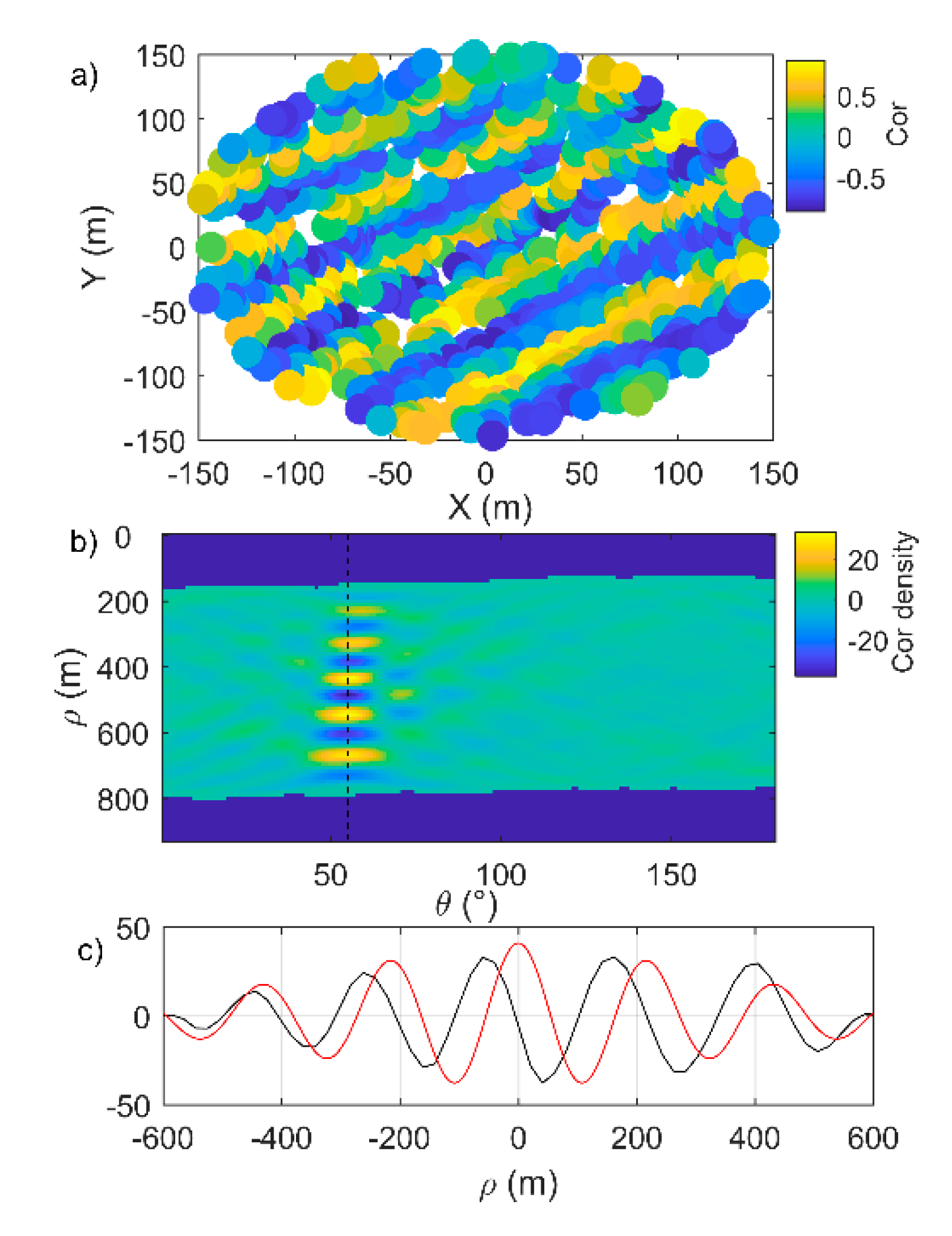
4.2.1. Correlation-Wavelet-Bathymetry (CWB) Method (Multi-Spectral)

The present example is based on the study described by [98]. The preliminary work of [99] has shown that it is possible to determine wave celerity directly from optical satellite imagery from the SPOT-5 sensor, thanks to the technical characteristics of the SPOT-5 satellite. A short temporal shift (2.04 s) exists between the acquisition of panchromatic and multispectral images, which makes it possible to calculate the celerity of waves between two instants by inter-band correlation. This represents an opportunity to locally identify several ( c , λ ) pairs in order to estimate the bathymetry using the dispersion relation.
The wave characteristics are extracted from the panchromatic and multi-spectral images of the SPOT-5 satellite by applying a wavelet analysis. It is noteworthy that the method can be generalized to any high resolution spaceborne sensor affected by small time-lags (e.g., between 0.5 s and 5 s) between bands (not only panchromatic and multi-spectral).
Thus, the methodology for estimating bathymetry is based on five steps:
  • Computation of the local wave spectra based on a wavelet analysis.
  • Extraction (based on the local spectrum) of N dominant waves characterized by their wavelengths λ n and directions θ n , n   [ 1 , N ] ;
  • For each dominant wave n , the estimation of the M celerities c n , m is associated to the wavelengths λ n , m included the wave-packet centered on λ n with the angle θ n . We therefore obtain a ( λ , c ) cloud associated to each dominant wave.
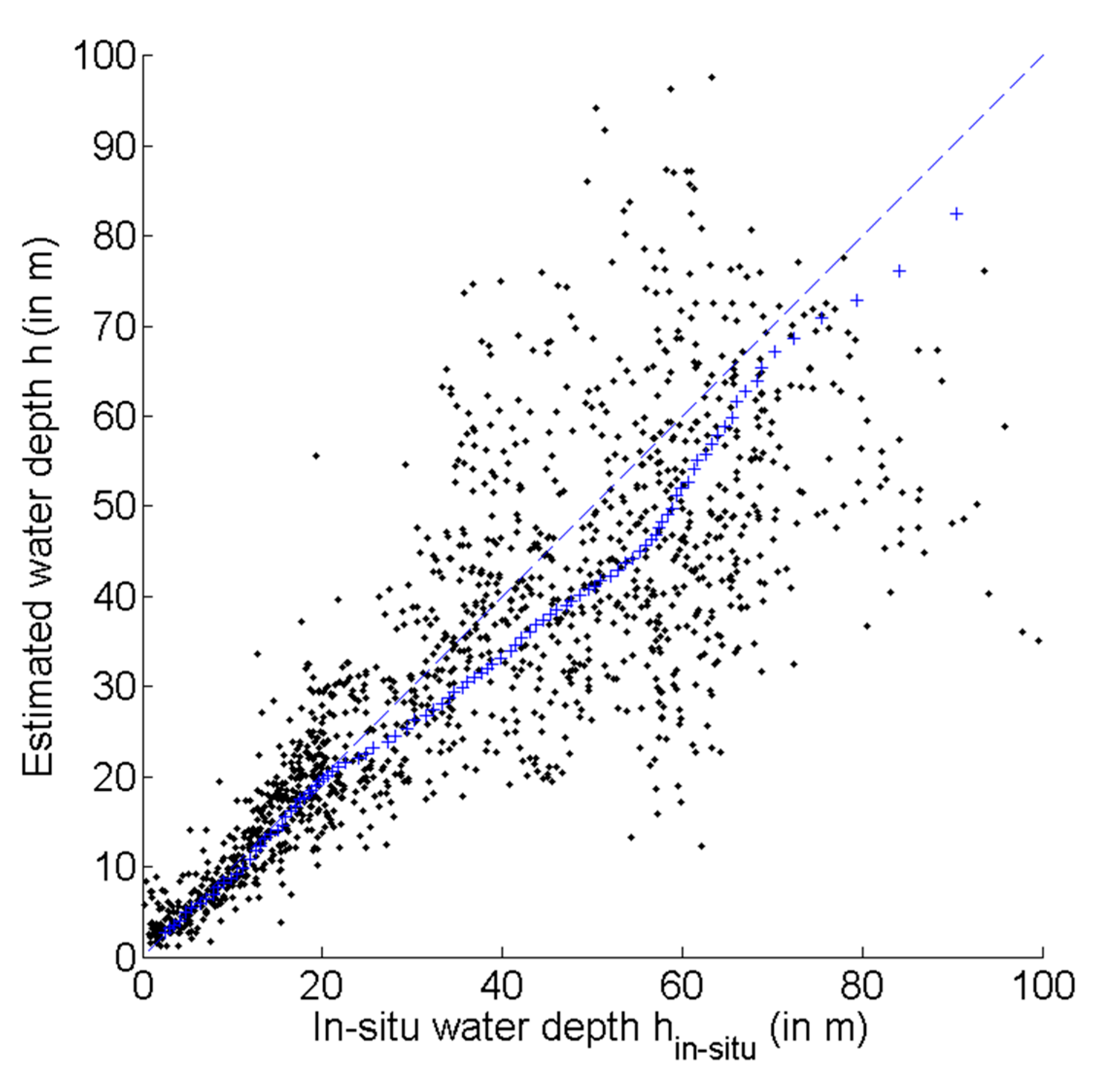
  • Use of the point cloud, M ( λ , c ) pairs to determine the water depth h n by fitting the dispersion curve (by least squares minimization).
  • Selection of the final depth h ^ among the h n computed for the N dominant waves based on the spectral energy associated to the corresponding waves.
The method has been validated using a SPOT-5 satellite acquisition taken on 6 February 2010 at 10:30 (1 h and 30 min before low tide) in the area of Saint Pierre, southwest of Reunion Island (Figure 9). The area of Saint Pierre is characterized by a narrow continental shelf and the current is negligible at the acquisition date (between 0.1 and 0.14 m/s (Navy Coastal Ocean Model of the National Oceanic and Atmospheric Administration)). This site was chosen because high resolution data were available.
The SPOT-5 satellite is equipped with high resolution sensors (HRG1-2) that allow the acquisition of multispectral (XS1-3) and panchromatic images (HMA) at resolutions of 10 and 2.5 m, respectively. The time difference between these images is 2.04 s. This configuration makes it possible to measure the displacements of pixel-sized features of the image [99]. The green band (XS1) of the multispectral image has been used for the correlation processing with the panchromatic image (HMA) because its bandwidth is centered on 0.55 microns, which was closer to the panchromatic image.
The bathymetry estimated by the CWB method was obtained at a spatial resolution of 20 m × 20 m Nevertheless, the actual resolution of the bathymetry cannot be so fine since the size of the sub-images used for the inter-correlation is 320 m × 320 m offshore and 160 m × 160 m near the coast, and these sub-images overlap each other. The bathymetry estimated by the CWBmethod was interpolated on a grid of 80 m × 80 m (Figure 10b).
The bathymetry results were compared with the in situ measurements (LiDAR data from LITTO3D products for depths shallower than 30 m and SHOM data obtained by multibeam echosounders for the largest depths), also interpolated on the grid of 80 m × 80 m (Figure 10a). To illustrate the quality of the method, Figure 11 shows the estimated bathymetry as a function of in situ bathymetry measurements. We can observe that dispersion is low up to hin-situ = 25 m but increases for deeper depths. In addition, the centiles (blue crosses on Figure 11) show that on average the method is particularly reliable over the in situ depth range [2 m, 25 m], then, a drift appears for depths larger than hin-situ = 25 m, reducing its accuracy.
The CWB method uses wavelet analysis coupled with an inter-band correlation calculation to determine N point clouds in the ( λ ,   c ) space, corresponding to dominant waves. The dispersion relation is then used to determine the water depths associated with these waves. Finally, the “best” estimated water depth is selected from an analysis of the energy spectra. This allows estimation of bathymetry from optical satellite imagery to a moderate degree of accuracy, namely a 20–30% error for a depth range of 3 to 80 m. The results may seem limited when compared to other existing methods to map bathymetry. Nevertheless, the method represents a real opportunity to estimate bathymetry where no other more conventional methods could be applied, while further developments are required to improve the accuracy of the method.
In [100], a Radon transform-based wave-pattern extraction and depth inversion method is presented. Wave patterns are extracted by applying a Radon transform and subsequent angle filtering to Sentinel-2 imagery, such that the wave signal contains the most-dominant wave directions. Depth is derived by exploiting the time-lag between color bands. The wave-phase per band, and after the phase shift, is obtained by applying a discrete Fourier transform to the Radon transform sinogram over a local sub-domain. In the study, depths were derived with good correlation, with good correlation of 0.82, and an RMSE of 2.58 m over the surveyed domain. These results are beyond the expectations, considering the challenging environment, including a deep-water canyon and its effect on surrounding wave patterns. In addition to the wave pattern enhancement and depth derivation, the Radon transform can be used to augment image resolution. Twenty meter resolution image bands, from Sentinel-2, were augmented to match the 10 m resolution bands, allowing those four extra bands to be used in the depth estimation method, with time-lags ranging between 1.005 s to 2.055 s [101].

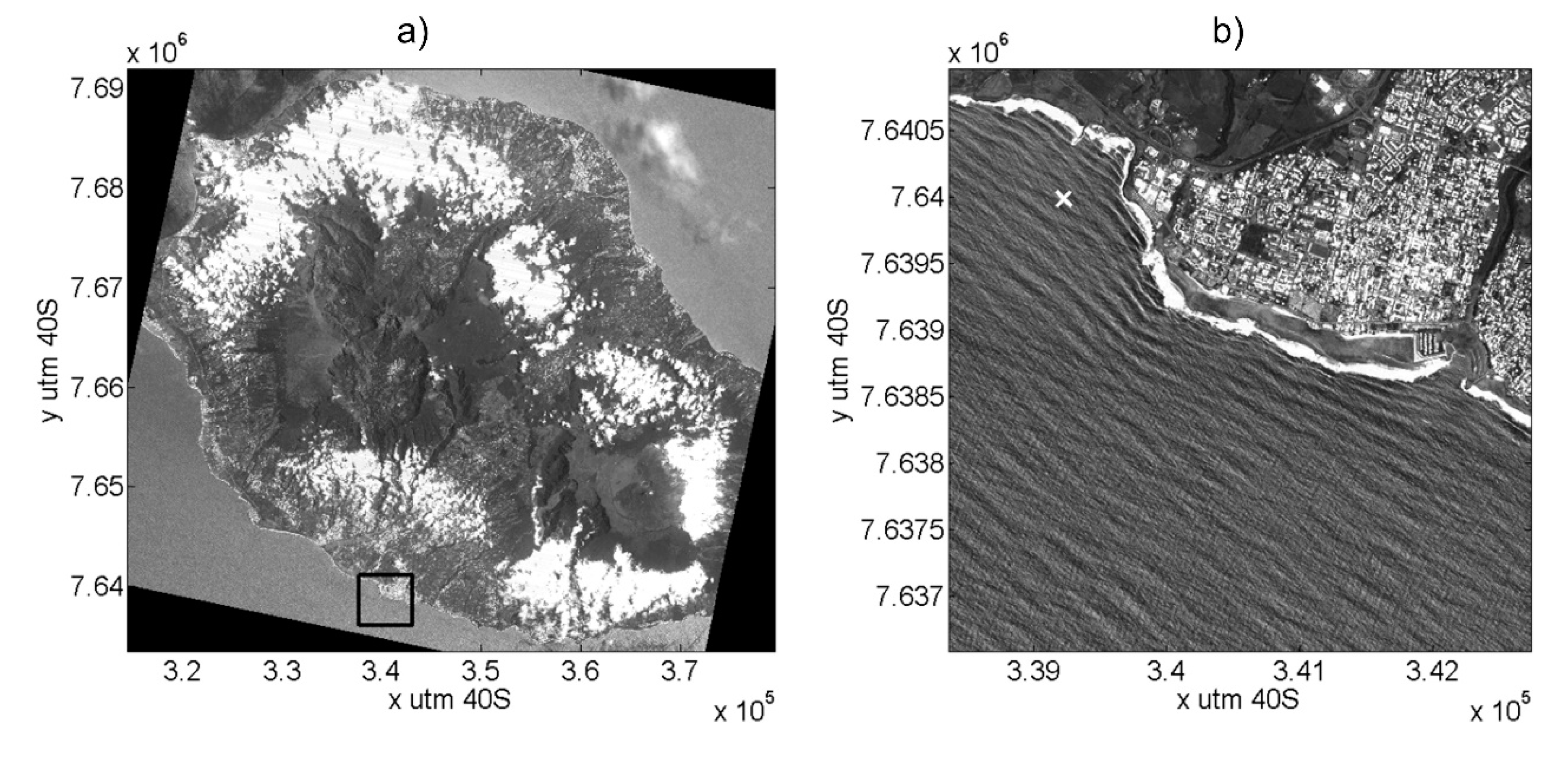
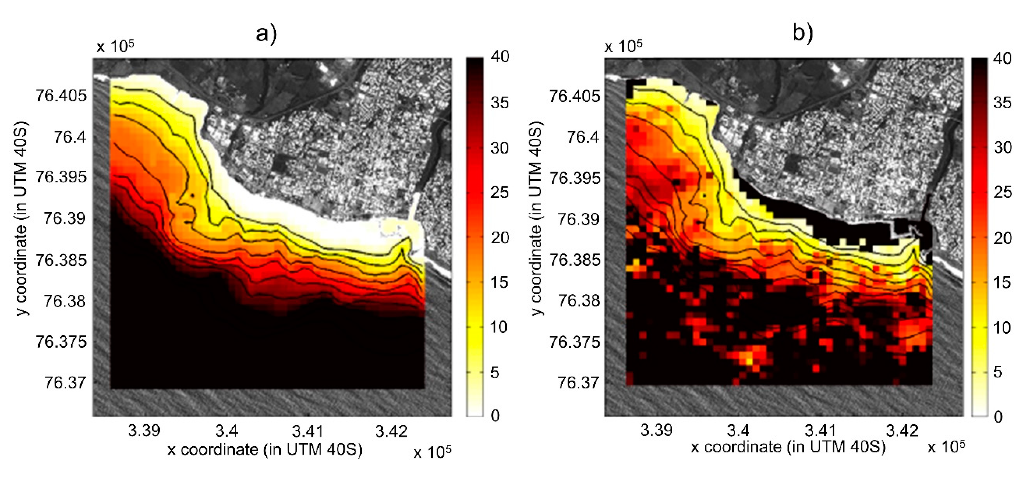
4.2.2. Video from Space: A Showcase with Pleiades Persistent Mode

In recent years, robust depth estimation methods through wave celerity inversion have been developed for shore-based video systems and drones [92,100,102,103], optimizing the information gathered in space and time (generally 10–20 min). At present, there are some pioneering works on video from space to recover coastal bathymetry [104,105,106] that clearly show the potential to derive waves from a sequence of images. Transposing advanced shore-based methodologies to satellite video imagery would provide a substantial gain over the bathymetry estimated by single or paired satellite imagery. There have been several implementations of these methods over the past 20 years, but not to spaceborne video. Almar et al. [107] show the capacity to derive depth using the sub-metric Pleiades satellite mission (Airbus/CNES) in persistent mode, which allows the acquisition of a sequence of images (12 images) at a regional scale (~100 km2) (Figure 12). To derive depths, a spatiotemporal cross-correlation method [108] for estimating wave velocity and inverse bathymetry is presented and applied to the 12-image sequence (Figure 13). Good agreement was found with in situ bathymetry measurements obtained during the COMBI 2017 Capbreton experiment (correlation of 0.8, RMSE = 1.4 m). Depth estimate saturation was found for depths >35 m in a deep canyon. The image sequence was used to study the sensitivity of the number of images. The results show that the accuracy increases with the number of images in the sequence and with a fine resolution.

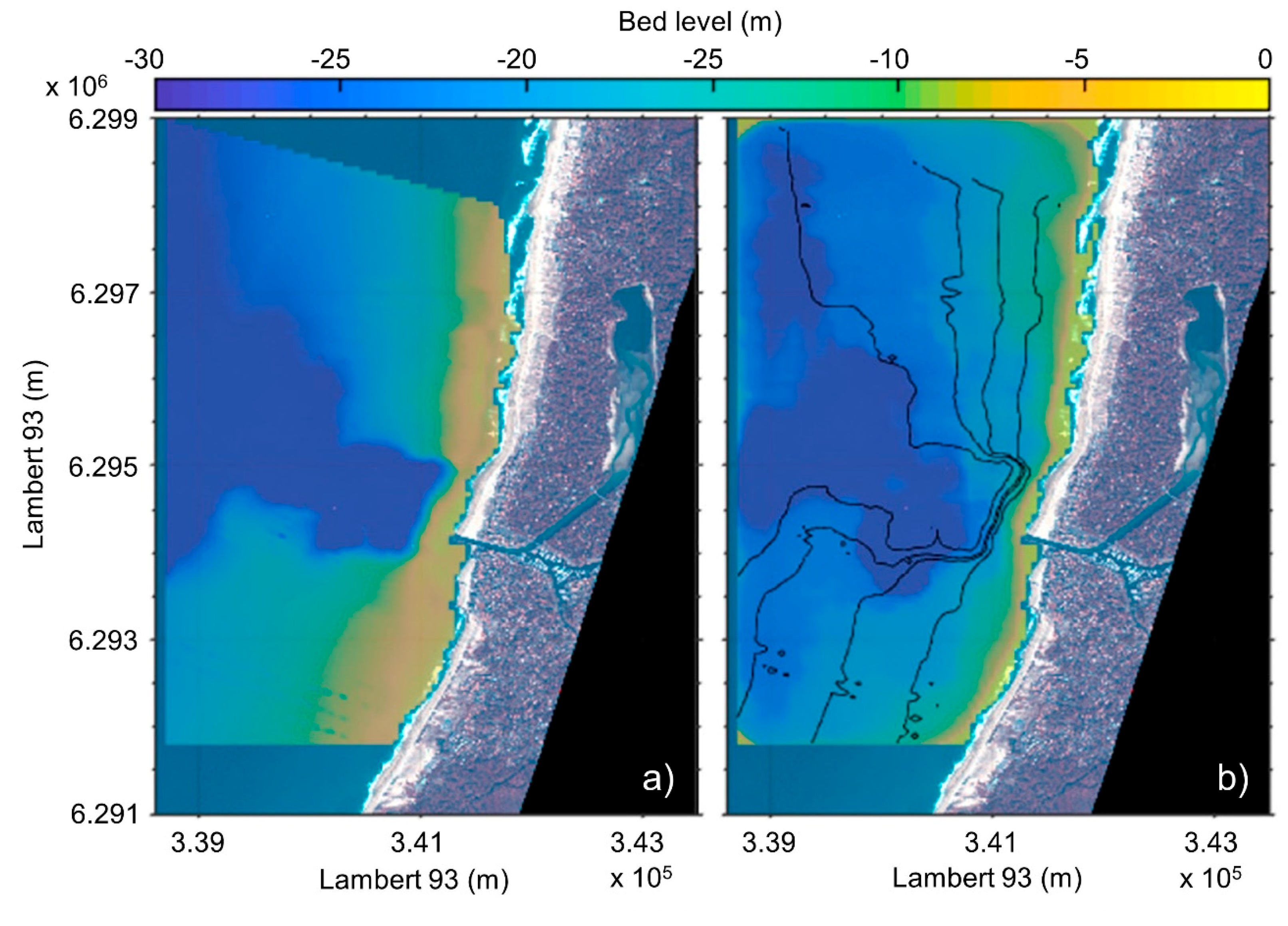
4.2.3. Synthetic Aperture Radar (SAR)

The computations of directional wave spectra by a fast Fourier transform (FFT) from the synthetic aperture radar (SAR) images have been used to retrieve the wavelength and wave direction, and to estimate the water depth by solving the linear dispersion relation (Equation (6)). The methodology calculates the 2D image spectrum in a cell of the image. The computation progress from open sea to shoreline in cells, which are either centered at fixed grid points [109] or along a wave ray [110], which allows tracking of the change in the wave length and wave direction as waves progress to the shore.
Brusch et al. [110] have attempted to establish the applicability of SAR data obtained from the commercially available TerraSAR-X data to two sites: Port Phillip in Australia and the Duck Research Pier in North Carolina, United States. The comparison of the results with local bathymetric data for depths between 2 and 40 m show a considerable dispersion, namely for shallower depths up to 10 m. Pleskachevsky et al. [21] explored the synergy and fusion of optical and SAR data for bathymetric estimation (radar data from TerraSAR-X and optical data from QuickBird satellite). Water depths between 20–60 m were obtained from the SAR-based method with an accuracy the in order of 15%. Mishra et al. [111] evaluated the applicability of SAR data obtained from the RISAT-1 C-band commercial products to a coastal region near Mumbai, India, and the obtained results qualitatively agree with available bathymetric information. Bian et al. [112] have developed a detection method based on swell patterns and the scattering mechanism using fully polarimetric SAR for the nearshore of Hainan Island, China. The comparison with navigational charts shows an average relative error of 9.73%, which improves the results obtained via single polarization SAR data. Pereira et al. [109] have applied Sentinel-1A with C-band SAR images to retrieve the bathymetry of the Aveiro (northwestern Portugal) study site. They have investigated the repeatability of the FFT methodology in retrieving the nearshore bathymetry, considering a set of four high temporal resolution images and analyzing the sensitivity of the results to internal factors related to the estimation of the wave length, either offshore or local. Their results show that a combined solution that merges the results of all the image set slightly improves the results. The relative error of the water depth ranges between 6% and 10% for water depths between 15 and 30 m.
Figure 14 presents a comparison between the ensemble calculated bathymetry using the Pereira et al. method [109] with in situ measurements. The computed values are averages for each cell and the results were obtained with the four SAR images. Figure 15 shows the computed versus measured dispersion for water depths between 10 and 35 m, showing large errors for higher water depths.

5. Summary of Methods

Table 1 presents the strengths, limitations, and accuracies associated with the different methods used for the retrieval of coastal topography and bathymetry.

6. Discussion

Various methods are widely used for the quantification of beach and intertidal topography and nearshore bathymetry, ranging from echosounder to LiDAR surveys, X-band radar images, photographic imagery, UAVs, and video systems. Land-based video camera systems have the ability to capture a large number of incident waves with multiple frames per second. Due to the duration of the videos, bathymetry errors are limited to tens of centimeters [113,114]. The same holds true for UAV applications. Both video systems and discrete bathymetric profiles have limited longshore spatial coverage and are not able to address nearshore bathymetry dynamics over large longshore distances (i.e., tens of kilometers). The satellite images which became available in the recent years (such as Sentinel-1 and more recently Sentinel-2), characterized by higher spatial and temporal resolution, can provide an optimal solution to retrieve the bathymetry using the different approaches presented above.

6.1. Beach Topography (Supratidal)

Stereoscopy would beneficiate from improvements in spatial resolution using pairs of panchromatic images acquired at sub-meter spatial resolutions, e.g., from sensors onboard the IKONOS (0.82 m), Quickbird (0.61 m), Pleiades (0.5 m), WorldView2 (0.5 m) GeoEye-1 (0.41 m), and WorldView 3–4 (0.31 m) satellite systems, and combining the data from these different systems. Recent results obtained using some of these datasets provide very accurate results (e.g., [115]). Nevertheless, the cost of acquisition of these images is one of the major drawbacks limiting their use [116].

6.2. Intertidal Topography

When using the waterline method, the frequent sampling of the Sentinel constellation helps to overcome the limitations induced by a shortage of images. The combined use of Sentinel-1 and -2 can provide an adequate number of images that covers the whole tidal cycle in a relatively short period. Figure 16 shows the coverage of the tidal cycle provided by Sentinel-1 (A and B) over the Arcachon Bay for a four-month period (June–September), enhanced by Sentinel-2 (A and B) free cloud images. As can be seen in Figure 16, the combination of acquisitions from Sentinel-1A, -1B, and -2A, -2B provides a very dense sampling of the tidal cycle, which could not be reached before.
Regarding the monitoring of intertidal areas with satellite radar altimetry, the use of SAR mode has proven to be more accurate than conventional altimeters. It was shown in [20] that CryoSat-2, when operating in SAR mode, provided more accurate intertidal topography profiles than the ERS-2 and ENVISAT conventional altimeters (the three sensors operate in the Ku-band). The use of radar altimetry to monitor intertidal topography can thus benefit from the SAR radar altimeters of the Sentinel-3 mission (Sentinel-3A and -3B). The Sentinel-3 SRAL (Synthetic aperture Radar ALtimeter) instrument is similar to that of CryoSat-2 (SIRAL), with an along-track resolution of about 300 m (350 m for CryoSat-2) [117]. In contrast to CryoSat-2, Sentinel-3 provides 100% SAR coverage. In addition to Sentinel-3 and in the continuity of the Jason satellite altimeter data services, another satellite radar altimetry mission is proposed, the Sentinel-6 mission, with two identical satellites (Jason-CS A and Jason-CS B) to be launched in 2020 and 2026 [118]. The mission will follow the orbit of the Jason altimetry missions [118] and it will therefore cover different regions than the ones covered by Sentinel-3. Sentinel-6 satellites will embark the Poseidon-4 radar altimeter [118]. The latter will operate simultaneously in pulse-width limited (LRM) and SAR modes, known as the interleaved mode, with a higher pulse repetition frequency of about 9 kHz, compared to conventional LRM altimeters. Two major advantages will be provided by the interleaved mode compared to the burst mode (transmit and receive alternatively) operating in SIRAL (CryoSat-2) and SRAL (Sentinel-3): (i) An increase in the along-track resolution and (ii) a reduction of the range measurement noise [118]. By means of satellite altimetry, more accurate results can be provided by the laser altimetry mission, ICESat-2 (Ice, Cloud, and Land Elevation Satellite-2), carrying only the advanced topographic laser altimeter system (ATLAS) instrument [119]. The ICESat-2 mission launched in September 15, 2018, [119], will not only provide a monitoring of glaciers and ice sheets topography but also the elevation of land surfaces (soil or vegetation canopy) and of coastal areas (sea surface, intertidal areas at low tide and possibly the bottom topography of shallow clear waters). The high accuracy provided by ICESat-2 is accompanied by a very high repetition rate of 10 kHz, equivalent to 0.7 m along-track sampling [119,120]. Employing the high repetition rate by ICESat-2 was enabled by using the micro-pulse photo-counting technology instead of the full-waveform approach of its predecessor, the ICESat mission, whose along-track sampling was equal to 170 m [119,121].
Other promising methods for intertidal bathymetry generation exist, for instance the one proposed by [122]. This method is based on a temporal correlation between the backscatter intensity of SAR images and the water level of the intertidal zone. It relies on a pixel-based algorithm and retrieves the intertidal bathymetry by modelling the temporal variability of pixel’s intensities by a logistic curve. The method’s first step is to discriminate between three classes based on their backscattering temporal variability characteristics, namely water (with a low temporal variability with low temporal average of backscattering coefficients), beach berm (with a low temporal variability with high temporal average of backscattering coefficients), and intertidal flats (with a high temporal variability). After discrimination, a final selection of intertidal pixels from the set of candidate pixels obtained by the first step is performed. This final selection is based on the following criterion: A correlation exists between the temporal evolution of the intensity of intertidal pixels and tidal stage (height), and this evolution can be modelled with the logistic function (pixels with backscattering coefficient profiles that cannot be modelled by this function are also eliminated by an automatic approach). The height of intertidal pixels is then computed by minimizing the following energy function:
E = i = 1 M { h i h t +   1 a ln ( J i k J i ) } 2 ,
where M is the number of images, h i is the tide height, h t is the terrain height at pixel (x, y), J i is the intensity at pixel (x, y), and a and k are the parameters of the logistic function. The major advantage of this method is the complete automatization of the procedure, with an estimated accuracy of 24 cm [122].

6.3. Nearshore Bathymetry (Subtidal)

The monitoring of submerged features in high energetic coastal regions requires remote sensing data with specific characteristics. Determining the swell properties in the wave field is the main feature from which a good spatial resolution remote sensing product is required, in order to be able to detect changes in the underwater topography. Repeatability is another crucial factor, since the production of merge solutions from a set of Sentinel images can improve the results. A good correlation between the bathymetric estimation from Sentinel-1 images and the observed bathymetry from in situ bathymetric measurements was observed, showing that the proposed approach can be successfully used and is relatively cost effective when compared with the previously mentioned methods.
In order to address the small-scale variability of under-water topography, a lot of studies investigate the potential of very high-resolution multispectral missions. However, to overcome the instrumental limitations (a low spectral resolution and noise-to-signal ratio) inherent in these sensors, recent developments focus on the use of multi-temporal and machine learning approaches to derive bathymetric maps in shallow waters. For example, various machine learning approaches have been employed, such as using artificial neural network (ANN) [123,124,125], support-vector machine (SVM) [126,127,128], and random forest (RF) [79,129] approaches. Good accuracies can be obtained using these methods, with RMSEs that can reach 35 cm by comparing to observations with high accuracies [126]. Furthermore, the benefits of the free and open multispectral mission data policy for many segments of society is widely demonstrated [130]. In particular, with its decametric resolution and 5-day repetitivity, the Sentinel-2 mission is recognized as one of the most promising data sources to provide satellite-derived bathymetry (SDB) at a worldwide scale. The development of algorithms and processes that use different sources of data could significantly improve the performances of SDB products.

6.4. Surface Water and Ocean Topography (SWOT)

The next-generation wide swath interferometric altimetry mission for surface water and ocean topography (SWOT) has great potential for coastal topographic and bathymetric mapping. Various techniques can be used, such as radar altimetry using SWOT nadir altimeter, the waterline method, and the inversion from wave characteristics using the collected SAR images, and potentially the InSAR method, which may be the most problematic, however. For the waterline method, one major advantage for using SWOT is that there is no need for tide gauge records or ocean modelling because SWOT will provide sea height information at high accuracy [131].

7. Conclusions

Coastal topography and bathymetry information are key parameters for several applications. Mapping the nearshore bathymetry and the foreshore topography is considered as an “observational priority” [7]. Their highly dynamic behavior requires frequent monitoring. Ground-, ship-, and airborne-based methods provide very accurate measurements, yet they lack the ability to provide repeated observations. Spaceborne-based methods are most suited to accomplish repeated observations while providing a large spatial coverage as well. This review focuses on spaceborne-based methods used for deriving topography and bathymetry in coastal environments. Various methods were described and illustrated, with examples including stereoscopy, the waterline method, InSAR, satellite radar altimetry, inversion from aquatic color data, and inversion from wave characteristics using multispectral and SAR data. The mentioned methods provide complementary data. Their combination can generate multisource bathymetry and topography products. Here, we separated the different methods in function of the coastal features that they were used for. However, many of them can be extended to other features. For instance, stereoscopy used for mapping beach topographies may be extended to intertidal areas using images acquired at low tides. The InSAR method used for intertidal topography mapping can be extended to beaches. The different methods used for nearshore bathymetry mapping may be extended to intertidal areas using images acquired at high tides. Therefore, an assessment of the potential and limitations of these different methods over different coastal features must be made. A comparison between these methods over the same study sites is also essential to obtain a concise knowledge about the difference in their performances (accuracy). The major limitation for spaceborne-based methods is meeting user requirements for vertical accuracy and further research must pursue this direction. With the advancements of remote sensing technologies and processing algorithms, better and more accurate monitoring can be expected in the future.

Author Contributions

F.F. conceived the review work; E.S. coordinated the writing; R.A., L.P.A., and E.B. supported the analysis, interpretation of the results and the writing referring to Section 2; G.H., E.S., and Z.L. supported the analysis, interpretation of the results and the writing referring to Section 3.1; E.S., and F.F. supported the writing of Section 3.2; E.S., F.F., I.T., and B.L. (Benoit Laignel) supported the analysis, interpretation of the results and the writing referring to Section 3.3; B.L. (Bertrand Lubac), S.C., and V.M. supported the analysis, interpretation of the results and the writing referring to Section 4.1; D.R., M.D., D.I., and A.P. supported the analysis, interpretation of the results and the writing referring to Section 4.2; P.B. and P.A.S. supported the analysis, interpretation of the results and the writing referring to Section 4.3; All the authors contributed to the discussion part and provided guidance and editing for the complete work.

Funding

This research was supported by the Centre National d’Etudes Spatiales (CNES). It is based on SWOT space mission and the SWOT COTEST and CTOH TOSCA projects and was also supported by the Normandy Region. EB is supported through a postdoctoral grant of the French Space Agency (CNES). Thanks, are also due to FCT/MCTES for the financial support to CESAM (UID/AMB/50017/2019), through Portuguese funds.

Conflicts of Interest

The authors declare no conflict of interest. The funders had no role in the design of the study; in the collection, analyses, or interpretation of data; in the writing of the manuscript, or in the decision to publish the results.

References

  1. Neumann, B.; Vafeidis, A.T.; Zimmermann, J.; Nicholls, R.J. Future Coastal Population Growth and Exposure to Sea-Level Rise and Coastal Flooding—A Global Assessment. PLoS ONE 2015, 10, e0118571. [Google Scholar] [CrossRef] [PubMed]
  2. CIESIN—Center for International Earth Science Information Network. Gridded Population of the World Version 3 (GPWv3); CIESIN: Palisades, NY, USA, 2005. [Google Scholar]
  3. Burkett, V.; Davidson, M. Coastal Impacts, Adaptation, and Vulnerabilities: A Technical Input to the 2012 National Climate Assessment. Cooperative Report to the 2013 National Climate Assessment; Island Press/Center for Resource Economics: Washington, DC, USA, 2012. [Google Scholar]
  4. Heege, T.; Bergin, M.; Hartmann, K.; Schenk, K. Satellite Services for Coastal Applications. In Ocean Solutions, Earth Solutions; Wright, D.J., Ed.; Esri Press: Redlands, CA, USA, 2016; pp. 357–368. [Google Scholar] [CrossRef]
  5. Nicholls, R.J.; Wong, P.P.; Burkett, V.R.; Codignotto, J.O.; Hay, J.E.; McLean, R.F.; Ragoonaden, S.; Woodroffe, C.D. Coastal Systems and Low-Lying Areas. In Climate Change 2007: Impacts, Adaptation and Vulnerability. Contribution of Working Group II to the Fourth Assessment Report of the Intergovernmental Panel on Climate Change; Parry, M.L., Canziani, O.F., Palutikof, J.P., van der Linden, P.J., Hanson, C.E., Eds.; Cambridge University Press: Cambridge, UK, 2007; pp. 315–356. [Google Scholar]
  6. Klemas, V.V. The Role of Remote Sensing in Predicting and Determining Coastal Storm Impacts. J. Coast. Res. 2009, 256, 1264–1275. [Google Scholar] [CrossRef]
  7. Benveniste, J.; Cazenave, A.; Vignudelli, S.; Fenoglio-Marc, L.; Shah, R.; Almar, R.; Andersen, O.; Birol, F.; Bonnefond, P.; Bouffard, J.; et al. Requirements for a Coastal Hazards Observing System. Front. Mar. Sci. 2019, 6, 348. [Google Scholar] [CrossRef]
  8. Mason, D.C.; Gurney, C.; Kennett, M. Beach Topography Mapping—A Comparison of Techniques. J. Coast. Conserv. 2000, 6, 113–124. [Google Scholar] [CrossRef]
  9. Holman, R.; Haller, M.C. Remote Sensing of the Nearshore. Ann. Rev. Mar. Sci. 2013, 5, 95–113. [Google Scholar] [CrossRef] [PubMed] [Green Version]
  10. Diaz, H.; Almar, R.; Bergsma, E.W.J.; Leger, F. On the Use of Satellite-Based Digital Elevation Models to Determine Coastal Topography. In Proceedings of the IGARSS 2019—2019 IEEE International Geoscience and Remote Sensing Symposium, Yokohama, Japan, 28 July–2 August 2019. [Google Scholar]
  11. Porskamp, P.; Rattray, A.; Young, M.; Ierodiaconou, D. Multiscale and Hierarchical Classification for Benthic Habitat Mapping. Geosciences 2018, 8, 119. [Google Scholar] [CrossRef]
  12. Janowski, L.; Trzcinska, K.; Tegowski, J.; Kruss, A.; Rucinska-Zjadacz, M.; Pocwiardowski, P. Nearshore Benthic Habitat Mapping Based on Multi-Frequency, Multibeam Echosounder Data Using a Combined Object-Based Approach: A Case Study from the Rowy Site in the Southern Baltic Sea. Remote Sens. 2018, 10, 1983. [Google Scholar] [CrossRef]
  13. Mielck, F.; Hass, H.C.; Betzler, C. High-Resolution Hydroacoustic Seafloor Classification of Sandy Environments in the German Wadden Sea. J. Coast. Res. 2014, 298, 1107–1117. [Google Scholar] [CrossRef]
  14. Madricardo, F.; Foglini, F.; Kruss, A.; Ferrarin, C.; Pizzeghello, N.M.; Murri, C.; Rossi, M.; Bajo, M.; Bellafiore, D.; Campiani, E.; et al. High Resolution Multibeam and Hydrodynamic Datasets of Tidal Channels and Inlets of the Venice Lagoon. Sci. Data 2017, 4, 170121. [Google Scholar] [CrossRef]
  15. Choi, C.; Kim, D. Optimum Baseline of a Single-Pass In-SAR System to Generate the Best DEM in Tidal Flats. IEEE J. Sel. Top. Appl. Earth Obs. Remote Sens. 2018, 11, 919–929. [Google Scholar] [CrossRef]
  16. Tateishi, R.; Akutsu, A. Relative DEM Production from SPOT Data without GCP. Int. J. Remote Sens. 1992, 13, 2517–2530. [Google Scholar] [CrossRef]
  17. Almeida, L.P.; Almar, R.; Bergsma, E.W.J.; Berthier, E.; Baptista, P.; Garel, E.; Dada, O.A.; Alves, B. Deriving High Spatial-Resolution Coastal Topography From Sub-Meter Satellite Stereo Imagery. Remote Sens. 2019, 11, 590. [Google Scholar] [CrossRef]
  18. Mason, D.C.; Davenport, I.J.; Robinson, G.J.; Flather, R.A.; Mccartney, B.S. Construction of an Inter-Tidal Digital Elevation Model by the “water-Line” Method. Geophys. Res. Lett. 1995, 22, 3187–3190. [Google Scholar] [CrossRef]
  19. Lee, S.K.; Ryu, J.H. High-Accuracy Tidal Flat Digital Elevation Model Construction Using TanDEM-X Science Phase Data. IEEE J. Sel. Top. Appl. Earth Obs. Remote Sens. 2017, 10, 2713–2724. [Google Scholar] [CrossRef]
  20. Salameh, E.; Frappart, F.; Marieu, V.; Spodar, A.; Parisot, J.P.; Hanquiez, V.; Turki, I.; Laignel, B. Monitoring Sea Level and Topography of Coastal Lagoons Using Satellite Radar Altimetry: The Example of the Arcachon Bay in the Bay of Biscay. Remote Sens. 2018, 10, 297. [Google Scholar] [CrossRef]
  21. Pleskachevsky, A.; Lehner, S.; Heege, T.; Mott, C. Synergy and Fusion of Optical and Synthetic Aperture Radar Satellite Data for Underwater Topography Estimation in Coastal Areas. Ocean Dyn. 2011, 61, 2099–2120. [Google Scholar] [CrossRef]
  22. Lyzenga, D.R. Passive Remote Sensing Techniques for Mapping Water Depth and Bottom Features. Appl. Opt. 1978, 17, 379. [Google Scholar] [CrossRef] [PubMed]
  23. Benny, A.H.; Dawson, G.J. Satellite Imagery as an Aid to Bathymetric Charting in the Red Sea. Cartogr. J. 1983, 20, 5–16. [Google Scholar] [CrossRef]
  24. Jupp, D.L.B.; Mayo, K.K.; Kuchler, D.A.; Claasen, D.V.R.; Kenchington, R.A.; Guerin, P.R. Remote Sensing for Planning and Managing the Great Barrier Reef of Australia. Photogrammetria 1985, 40, 21–42. [Google Scholar] [CrossRef]
  25. Lyzenga, D.R. Remote Sensing of Bottom Reflectance and Water Attenuation Parameters in Shallow Water Using Aircraft and Landsat Data. Int. J. Remote Sens. 1981, 2, 71–82. [Google Scholar] [CrossRef]
  26. Lyzenga, D.R. Shallow-Water Bathymetry Using Combined Lidar and Passive Multispectral Scanner Data. Int. J. Remote Sens. 1985, 6, 115–125. [Google Scholar] [CrossRef]
  27. Alpers, W.; Hennings, I. A Theory of the Imaging Mechanism of Underwater Bottom Topography by Real and Synthetic Aperture Radar. J. Geophys. Res. 1984, 89, 10529. [Google Scholar] [CrossRef]
  28. Colomina, I.; Molina, P. Unmanned Aerial Systems for Photogrammetry and Remote Sensing: A Review. ISPRS J. Photogramm. Remote Sens. 2014, 92, 79–97. [Google Scholar] [CrossRef]
  29. Mancini, F.; Dubbini, M.; Gattelli, M.; Stecchi, F.; Fabbri, S.; Gabbianelli, G.; Mancini, F.; Dubbini, M.; Gattelli, M.; Stecchi, F.; et al. Using Unmanned Aerial Vehicles (UAV) for High-Resolution Reconstruction of Topography: The Structure from Motion Approach on Coastal Environments. Remote Sens. 2013, 5, 6880–6898. [Google Scholar] [CrossRef] [Green Version]
  30. Gonçalves, J.A.; Henriques, R. UAV Photogrammetry for Topographic Monitoring of Coastal Areas. ISPRS J. Photogramm. Remote Sens. 2015, 104, 101–111. [Google Scholar] [CrossRef]
  31. Niethammer, U.; James, M.R.; Rothmund, S.; Travelletti, J.; Joswig, M. UAV-Based Remote Sensing of the Super-Sauze Landslide: Evaluation and Results. Eng. Geol. 2012, 128, 2–11. [Google Scholar] [CrossRef]
  32. Gleyzes, J.P.; Meygret, A.; Fratter, C.; Panem, C.; Baillarin, S.; Valorge, C. SPOT5: System Overview and Image Ground Segment. In Proceedings of the IGARSS 2003—2003 IEEE International Geoscience and Remote Sensing Symposium, Toulouse, France, 21–25 July 2003; pp. 300–302. [Google Scholar] [CrossRef]
  33. Panagiotakis, E.; Chrysoulakis, N.; Charalampopoulou, V.; Poursanidis, D.; Panagiotakis, E.; Chrysoulakis, N.; Charalampopoulou, V.; Poursanidis, D. Validation of Pleiades Tri-Stereo DSM in Urban Areas. ISPRS Int. J. Geo-Inf. 2018, 7, 118. [Google Scholar] [CrossRef]
  34. Mason, D.C.; Davenport, I.J. Accurate and Efficient Determination of the Shoreline in ERS-1 SAR Images. IEEE Trans. Geosci. Remote Sens. 1996, 34, 1243–1253. [Google Scholar] [CrossRef]
  35. Mason, D.C.; Davenport, I.J.; Flather, R.A. Interpolation of an Intertidal Digital Elevation Model from Heighted Shorelines: A Case Study in the Western Wash. Estuar. Coast. Shelf Sci. 1997, 45, 599–612. [Google Scholar] [CrossRef]
  36. Heygster, G.; Dannenberg, J.; Notholt, J. Topographic Mapping of the German Tidal Flats Analyzing SAR Images With the Waterline Method. IEEE Trans. Geosci. Remote Sens. 2010, 48, 1019–1030. [Google Scholar] [CrossRef]
  37. Li, Z.; Heygster, G.; Notholt, J. Intertidal Topographic Maps and Morphological Changes in the German Wadden Sea between 1996–1999 and 2006–2009 from the Waterline Method and SAR Images. IEEE J. Sel. Top. Appl. Earth Obs. Remote Sens. 2014, 7, 3210–3224. [Google Scholar] [CrossRef]
  38. Touzi, R.; Lopes, A.; Bousquet, P. A Statistical and Geometrical Edge Detector for SAR Images. IEEE Trans. Geosci. Remote Sens. 1988, 26, 764–773. [Google Scholar] [CrossRef]
  39. Niedermeier, A.; Romaneeßen, E.; Lehner, S. Detection of Coastlines in SAR Images Using Wavelet Methods. IEEE Trans. Geosci. Remote Sens. 2000, 38, 2270–2281. [Google Scholar] [CrossRef]
  40. Mallat, S.; Zhong, S. Characterization of Signals from Multiscale Edges. IEEE Trans. Pattern Anal. Mach. Intell. 1992, 14, 710–732. [Google Scholar] [CrossRef]
  41. Xu, Z.; Kim, D.; Kim, S.H.; Cho, Y.K.; Lee, S.G. Estimation of Seasonal Topographic Variation in Tidal Flats Using Waterline Method: A Case Study in Gomso and Hampyeong Bay, South Korea. Estuar. Coast. Shelf Sci. 2016, 183, 213–220. [Google Scholar] [CrossRef]
  42. Sibson, R. A Brief Description of Natural Neighbour Interpolation. In Interpreting Multivariate Data; John Wiley & Sons: New York, NY, USA, 1981; pp. 21–36. [Google Scholar]
  43. Mason, D.C.; Amin, M.; Davenport, I.J.; Flather, R.A.; Robinson, G.J.; Smith, J.A. Measurement of Recent Intertidal Sediment Transport in Morecambe Bay Using the Waterline Method. Estuar. Coast. Shelf Sci. 1999, 49, 427–456. [Google Scholar] [CrossRef]
  44. Wu, D.; Du, Y.; Su, F.; Huang, W.; Zhang, L. An Improved DEM Construction Method For Mudflats Based on BJ-1 Small Satellite Images: A Case Study on Bohai Bay. ISPRS Int. Arch. Photogramm. Remote Sens. Spat. Inf. Sci. 2018, 1871–1878. [Google Scholar] [CrossRef]
  45. Mason, D.C.; Davenport, I.J.; Flather, R.A.; Gurney, C.; Robinson, G.J.; Smith, J.A. A Sensitivity Analysis of the Waterline Method of Constructing a Digital Elevation Model for Intertidal Areas in ERS SAR Scene of Eastern England. Estuar. Coast. Shelf Sci. 2001, 53, 759–778. [Google Scholar] [CrossRef]
  46. Mason, D.C.; Scott, T.R.; Dance, S.L. Remote Sensing of Intertidal Morphological Change in Morecambe Bay, U.K., between 1991 and 2007. Estuar. Coast. Shelf Sci. 2010, 87, 487–496. [Google Scholar] [CrossRef]
  47. Li, Z. Morphological Development of the German Wadden Sea from 1996 to 2009 Determined with Waterline Method and SAR and Landsat Satellite Images. Ph.D. Thesis, Dept. of Physics and Electrical Engineering, Universität Bremen, Bremen, Germany, 2014. [Google Scholar]
  48. Wahl, T.; Haigh, I.D.; Woodworth, P.L.; Albrecht, F.; Dillingh, D.; Jensen, J.; Nicholls, R.J.; Weisse, R.; Wöppelmann, G. Observed Mean Sea Level Changes around the North Sea Coastline from 1800 to Present. Earth-Sci. Rev. 2013, 124, 51–67. [Google Scholar] [CrossRef]
  49. Li, F.K.; Goldstein, R.M. Studies of Multibaseline Spaceborne Interferometric Synthetic Aperture Radars. IEEE Trans. Geosci. Remote Sens. 1990, 28, 88–97. [Google Scholar] [CrossRef]
  50. Simons, M.; Rosen, P. Interferometric Synthetic Aperture Radar Geodesy. In Treatise on Geophysics; Schubert, G., Ed.; Elsevier: Amsterdam, The Netherlands, 2007; pp. 391–446. [Google Scholar] [CrossRef]
  51. Rosen, P.A.; Hensley, S.; Joughin, I.R.; Li, F.; Madsen, S.N.; Rodriguez, E.; Goldstein, R.M. Synthetic Aperture Radar Interferometry. IEEE Proc. 2000, 88, 333–382. [Google Scholar] [CrossRef]
  52. Moreira, A.; Prats-Iraola, P.; Younis, M.; Krieger, G.; Hajnsek, I.; Papathanassiou, K.P. A Tutorial on Synthetic Aperture Radar. IEEE Geosci. Remote Sens. Mag. 2013, 1, 6–43. [Google Scholar] [CrossRef]
  53. Bamler, R.; Hartl, P. Synthetic Aperture Radar Interferometry. Inverse Probl. 1998, 14, R1–R54. [Google Scholar] [CrossRef]
  54. Bürgmann, R.; Rosen, P.A.; Fielding, E.J. Synthetic Aperture Radar Interferometry to Measure Earth’s Surface Topography and Its Deformation. Annu. Rev. Earth Planet. Sci. 2000, 28, 169–209. [Google Scholar] [CrossRef]
  55. Gens, R.; Van Genderen, J.L. Review Article SAR Interferometry—Issues, Techniques, Applications. Int. J. Remote Sens. 1996, 17, 1803–1835. [Google Scholar] [CrossRef]
  56. Won, J.S.; Kim, S.W. ERS SAR Interferometry for Tidal Flat DEM. In Proceedings of the FRINGE 2003 Workshop, Frascati, Italy, 1–5 December 2003. [Google Scholar]
  57. Zebker, H.A.; Villasenor, J. Decorrelation in Interferometric Radar Echoes. IEEE Trans. Geosci. Remote Sens. 1992, 30, 950–959. [Google Scholar] [CrossRef]
  58. Just, D.; Bamler, R. Phase Statistics of Interferograms with Applications to Synthetic Aperture Radar. Appl. Opt. 1994, 33, 4361. [Google Scholar] [CrossRef]
  59. Gade, M.; Alpers, W.; Melsheimer, C.; Tanck, G. Classification of Sediments on Exposed Tidal Flats in the German Bight Using Multi-Frequency Radar Data. Remote Sens. Environ. 2008, 112, 1603–1613. [Google Scholar] [CrossRef]
  60. Wingham, D.J.; Rapley, C.G.; Griffiths, H. New Techniques in Satellite Altimeter Tracking Systems. In Proceedings of the IGARSS 86 Symposium, Zurich, Switzerland, 8–11 Sertember 1986; pp. 1339–1344. [Google Scholar]
  61. Frappart, F.; Calmant, S.; Cauhopé, M.; Seyler, F.; Cazenave, A. Preliminary Results of ENVISAT RA-2-Derived Water Levels Validation over the Amazon Basin. Remote Sens. Environ. 2006, 100, 252–264. [Google Scholar] [CrossRef]
  62. Frappart, F.; Papa, F.; Marieu, V.; Malbeteau, Y.; Jordy, F.; Calmant, S.; Durand, F.; Bala, S. Preliminary Assessment of SARAL/AltiKa Observations over the Ganges-Brahmaputra and Irrawaddy Rivers. Mar. Geod. 2015, 38, 568–580. [Google Scholar] [CrossRef]
  63. Normandin, C.; Frappart, F.; Diepkilé, A.T.; Marieu, V.; Mougin, E.; Blarel, F.; Lubac, B.; Braquet, N.; Ba, A.; Normandin, C.; et al. Evolution of the Performances of Radar Altimetry Missions from ERS-2 to Sentinel-3A over the Inner Niger Delta. Remote Sens. 2018, 10, 833. [Google Scholar] [CrossRef]
  64. Bonnefond, P.; Verron, J.; Aublanc, J.; Babu, K.; Bergé-Nguyen, M.; Cancet, M.; Chaudhary, A.; Crétaux, J.F.; Frappart, F.; Haines, B.; et al. The Benefits of the Ka-Band as Evidenced from the SARAL/AltiKa Altimetric Mission: Quality Assessment and Unique Characteristics of AltiKa Data. Remote Sens. 2018, 10, 83. [Google Scholar] [CrossRef]
  65. Mouw, C.B.; Greb, S.; Aurin, D.; DiGiacomo, P.M.; Lee, Z.; Twardowski, M.; Binding, C.; Hu, C.; Ma, R.; Moore, T.; et al. Aquatic Color Radiometry Remote Sensing of Coastal and Inland Waters: Challenges and Recommendations for Future Satellite Missions. Remote Sens. Environ. 2015, 160, 15–30. [Google Scholar] [CrossRef]
  66. IOCCG. Remote Sensing of Ocean Colour in Coastal, and Other Optically Complex, Waters; Reports of the International Ocean-Colour Coordinating Group, No. 3; Sathyendranath, S., Ed.; IOCCG: Dartmouth, NS, Canada, 2000. [Google Scholar]
  67. Capo, S.; Lubac, B.; Marieu, V.; Robinet, A.; Bru, D.; Bonneton, P. Assessment of the Decadal Morphodynamic Evolution of a Mixed Energy Inlet Using Ocean Color Remote Sensing. Ocean Dyn. 2014, 64, 1517–1530. [Google Scholar] [CrossRef]
  68. Petit, T.; Bajjouk, T.; Mouquet, P.; Rochette, S.; Vozel, B.; Delacourt, C. Hyperspectral Remote Sensing of Coral Reefs by Semi-Analytical Model Inversion—Comparison of Different Inversion Setups. Remote Sens. Environ. 2017, 190, 348–365. [Google Scholar] [CrossRef]
  69. Philpot, W.D. Bathymetric Mapping with Passive Multispectral Imagery. Appl. Opt. 1989, 28, 1569. [Google Scholar] [CrossRef]
  70. Maritorena, S.; Morel, A.; Gentili, B. Diffuse Reflectance of Oceanic Shallow Waters: Influence of Water Depth and Bottom Albedo. Limnol. Oceanogr. 1994, 39, 1689–1703. [Google Scholar] [CrossRef]
  71. Lee, Z.; Carder, K.L.; Mobley, C.D.; Steward, R.G.; Patch, J.S. Hyperspectral Remote Sensing for Shallow Waters: 2 Deriving Bottom Depths and Water Properties by Optimization. Appl. Opt. 1999, 38, 3831. [Google Scholar] [CrossRef]
  72. Albert, A.; Gege, P. Inversion of Irradiance and Remote Sensing Reflectance in Shallow Water between 400 and 800 Nm for Calculations of Water and Bottom Properties. Appl. Opt. 2006, 45, 2331. [Google Scholar] [CrossRef]
  73. Lyzenga, D.R.; Malinas, N.P.; Tanis, F.J. Multispectral Bathymetry Using a Simple Physically Based Algorithm. IEEE Trans. Geosci. Remote Sens. 2006, 44, 2251–2259. [Google Scholar] [CrossRef]
  74. Bramante, J.F.; Raju, D.K.; Sin, T.M. Multispectral Derivation of Bathymetry in Singapore’s Shallow, Turbid Waters. Int. J. Remote Sens. 2013, 34, 2070–2088. [Google Scholar] [CrossRef]
  75. Dekker, A.G.; Phinn, S.R.; Anstee, J.; Bissett, P.; Brando, V.E.; Casey, B.; Fearns, P.; Hedley, J.; Klonowski, W.; Lee, Z.P.; et al. Intercomparison of Shallow Water Bathymetry, Hydro-Optics, and Benthos Mapping Techniques in Australian and Caribbean Coastal Environments. Limnol. Oceanogr. Methods 2011, 9, 396–425. [Google Scholar] [CrossRef]
  76. Su, H.; Liu, H.; Heyman, W.D. Automated Derivation of Bathymetric Information from Multi-Spectral Satellite Imagery Using a Non-Linear Inversion Model. Mar. Geod. 2008, 31, 281–298. [Google Scholar] [CrossRef]
  77. Stumpf, R.P.; Holderied, K.; Sinclair, M. Determination of Water Depth with High-Resolution Satellite Imagery over Variable Bottom Types. Limnol. Oceanogr. 2003, 48, 547–556. [Google Scholar] [CrossRef]
  78. Evagorou, E.G.; Mettas, C.; Agapiou, A.; Themistocleous, K.; Hadjimitsis, D.G. Bathymetric Maps from Multi-Temporal Analysis of Sentinel-2 Data: The Case Study of Limassol, Cyprus. Adv. Geosci. 2019, 45, 397–407. [Google Scholar] [CrossRef]
  79. Sagawa, T.; Yamashita, Y.; Okumura, T.; Yamanokuchi, T.; Sagawa, T.; Yamashita, Y.; Okumura, T.; Yamanokuchi, T. Satellite Derived Bathymetry Using Machine Learning and Multi-Temporal Satellite Images. Remote Sens. 2019, 11, 1155. [Google Scholar] [CrossRef]
  80. Gordon, H.R.; Brown, O.B.; Evans, R.H.; Brown, J.W.; Smith, R.C.; Baker, K.S.; Clark, D.K. A Semianalytic Radiance Model of Ocean Color. J. Geophys. Res. Atmos. 1988, 93, 10909–10924. [Google Scholar] [CrossRef]
  81. Lee, Z.; Shang, S.; Qi, L.; Yan, J.; Lin, G. A Semi-Analytical Scheme to Estimate Secchi-Disk Depth from Landsat-8 Measurements. Remote Sens. Environ. 2016, 177, 101–106. [Google Scholar] [CrossRef]
  82. Lee, Z.; Lubac, B.; Werdell, J.; Arnone, R. An Update of the Quasi-Analytical Algorithm (QAA_v5). In International Ocean Color Group Software Report; IOCCG: Dartmouth, NS, Canada, 2009; pp. 1–9. [Google Scholar]
  83. Lee, Z.; Hu, C.; Shang, S.; Du, K.; Lewis, M.; Arnone, R.; Brewin, R. Penetration of UV-Visible Solar Radiation in the Global Oceans: Insights from Ocean Color Remote Sensing. J. Geophys. Res. Ocean. 2013, 118, 4241–4255. [Google Scholar] [CrossRef]
  84. Vanhellemont, Q.; Ruddick, K. Advantages of High Quality SWIR Bands for Ocean Colour Processing: Examples from Landsat-8. Remote Sens. Environ. 2015, 161, 89–106. [Google Scholar] [CrossRef]
  85. Novoa, S.; Doxaran, D.; Ody, A.; Vanhellemont, Q.; Lafon, V.; Lubac, B.; Gernez, P.; Novoa, S.; Doxaran, D.; Ody, A.; et al. Atmospheric Corrections and Multi-Conditional Algorithm for Multi-Sensor Remote Sensing of Suspended Particulate Matter in Low-to-High Turbidity Levels Coastal Waters. Remote Sens. 2017, 9, 61. [Google Scholar] [CrossRef]
  86. Ilori, C.; Pahlevan, N.; Knudby, A.; Ilori, C.O.; Pahlevan, N.; Knudby, A. Analyzing Performances of Different Atmospheric Correction Techniques for Landsat 8: Application for Coastal Remote Sensing. Remote Sens. 2019, 11, 469. [Google Scholar] [CrossRef]
  87. Bru, D.; Lubac, B.; Normandin, C.; Robinet, A.; Leconte, M.; Hagolle, O.; Martiny, N.; Jamet, C.; Bru, D.; Lubac, B.; et al. Atmospheric Correction of Multi-Spectral Littoral Images Using a PHOTONS/AERONET-Based Regional Aerosol Model. Remote Sens. 2017, 9, 814. [Google Scholar] [CrossRef]
  88. Wettle, M.; Brando, V.E.; Dekker, A.G. A Methodology for Retrieval of Environmental Noise Equivalent Spectra Applied to Four Hyperion Scenes of the Same Tropical Coral Reef. Remote Sens. Environ. 2004, 93, 188–197. [Google Scholar] [CrossRef]
  89. Botha, E.; Brando, V.; Dekker, A.; Botha, E.J.; Brando, V.E.; Dekker, A.G. Effects of Per-Pixel Variability on Uncertainties in Bathymetric Retrievals from High-Resolution Satellite Images. Remote Sens. 2016, 8, 459. [Google Scholar] [CrossRef]
  90. IOCCG. Remote Sensing of Inherent Optical Properties: Fundamentals, Tests of Algorithms, and Applications; Reports of the InternationalOcean-Colour Coordinating Group, No. 5; Lee, Z., Ed.; IOCCG: Dartmouth, NS, Canada, 2006. [Google Scholar]
  91. Lee, Z.; Arnone, R.; Hu, C.; Werdell, P.J.; Lubac, B. Uncertainties of Optical Parameters and Their Propagations in an Analytical Ocean Color Inversion Algorithm. Appl. Opt. 2010, 49, 369. [Google Scholar] [CrossRef]
  92. Bergsma, E.W.J.; Almar, R. Video-Based Depth Inversion Techniques, a Method Comparison with Synthetic Cases. Coast. Eng. 2018, 138, 199–209. [Google Scholar] [CrossRef]
  93. Holland, T.K. Application of the Linear Dispersion Relation with Respect to Depth Inversion and Remotely Sensed Imagery. IEEE Trans. Geosci. Remote Sens. 2001, 39, 2060–2072. [Google Scholar] [CrossRef]
  94. Stockdon, H.F.; Holman, R.A. Estimation of Wave Phase Speed and Nearshore Bathymetry from Video Imagery. J. Geophys. Res. Ocean. 2000, 105, 22015–22033. [Google Scholar] [CrossRef]
  95. Catálan, P.A.; Haller, M.C. Remote Sensing of Breaking Wave Phase Speeds with Application to Non-Linear Depth Inversions. Coast. Eng. 2008, 55, 93–111. [Google Scholar] [CrossRef]
  96. Leu, L.G.; Chang, H.W. Remotely Sensing in Detecting the Water Depths and Bed Load of Shallow Waters and Their Changes. Ocean Eng. 2005, 32, 1174–1198. [Google Scholar] [CrossRef]
  97. Marieu, V.; Guerin, T.; Capo, S.; Bru, D.; Lubac, B.; Hanquiez, V.; Lafon, V.; Bonneton, P. Bathymétrie de l’embouchure Du Bassin d’Arcachon Par Fusion de Données Hétéroclites et Reconstruction Bathymétrique. In Proceedings of the XIIèmes Journées Nationales Génie Côtier—Génie Civil, Cherbourg, France, 12–14 June 2012. [Google Scholar] [CrossRef]
  98. Poupardin, A.; Idier, D.; de Michele, M.; Raucoules, D. Water Depth Inversion From a Single SPOT-5 Dataset. IEEE Trans. Geosci. Remote Sens. 2016, 54, 2329–2342. [Google Scholar] [CrossRef]
  99. De Michele, M.; Leprince, S.; Thiébot, J.; Raucoules, D.; Binet, R. Direct Measurement of Ocean Waves Velocity Field from a Single SPOT-5 Dataset. Remote Sens. Environ. 2012, 119, 266–271. [Google Scholar] [CrossRef]
  100. Bergsma, E.W.J.; Almar, R.; Maisongrande, P. Radon-Augmented Sentinel-2 Satellite Imagery to Derive Wave-Patterns and Regional Bathymetry. Remote Sens. 2019, 11, 1918. [Google Scholar] [CrossRef]
  101. Bergsma, E.W.J.; Almar, R.; Maisongrande, P. Radon-Augmentation of Sentinel-II Imagery to Enhance Resolution and Visibility of (Nearshore) Ocean-Wave Patterns. In Proceedings of the IGARSS 2019—2019 IEEE International Geoscience and Remote Sensing Symposium, Yokohama, Japan, 28 July–2 August 2019. [Google Scholar]
  102. Matsuba, Y.; Sato, S. Nearshore Bathymetry Estimation Using UAV. Coast. Eng. J. 2018, 60, 51–59. [Google Scholar] [CrossRef]
  103. Holman, R.A.; Brodie, K.L.; Spore, N.J. Surf Zone Characterization Using a Small Quadcopter: Technical Issues and Procedures. IEEE Trans. Geosci. Remote Sens. 2017, 55, 2017–2027. [Google Scholar] [CrossRef]
  104. Abileah, R. Mapping Shallow Water Depth from Satellite. In Proceedings of the ASPRS Annual Conference, Reno, NV, USA, 1–5 May 2006. [Google Scholar]
  105. McCarthy, B.L. Coastal Bathymetry Using 8-Color Multispectral Satellite Observation of Wave Motion; Naval Postgraduate School: Monterey, CA, USA, 2010. [Google Scholar]
  106. Myrick, I.I.; Kenneth, B. Coastal Bathymetry Using Satellite Observation in Support of Intelligence Preparation of the Environment; Naval Postgraduate School: Monterey, CA, USA, 2011. [Google Scholar]
  107. Almar, R.; Bergsma, E.W.J.; Maisongrande, P.; de Almeida, L.P.M. Wave-Derived Coastal Bathymetry from Satellite Video Imagery: A Showcase with Pleiades Persistent Mode. Remote Sens. Environ. 2019, 231, 111263. [Google Scholar] [CrossRef]
  108. Almar, R.; Bergsma, E.W.J.; Maisongrande, P.; Giros, A.; Almeida, L.P. On the Application of a Two-Dimension Spatio-Temporal Cross-Correlation Method to Inverse Coastal Bathymetry from Waves Using a Satellite-Based Video Sequence. In Proceedings of the IGARSS 2019—2019 IEEE International Geoscience and Remote Sensing Symposium, Yokohama, Japan, 28 July–2 August 2019. [Google Scholar]
  109. Pereira, P.; Baptista, P.; Cunha, T.; Silva, P.A.; Romão, S.; Lafon, V. Estimation of the Nearshore Bathymetry from High Temporal Resolution Sentinel-1A C-Band SAR Data—A Case Study. Remote Sens. Environ. 2019, 223, 166–178. [Google Scholar] [CrossRef]
  110. Brusch, S.; Held, P.; Lehner, S.; Rosenthal, W.; Pleskachevsky, A. Underwater Bottom Topography in Coastal Areas from TerraSAR-X Data. Int. J. Remote Sens. 2011, 32, 4527–4543. [Google Scholar] [CrossRef]
  111. Mishra, M.K.; Ganguly, D.; Chauhan, P. Estimation of Coastal Bathymetry Using RISAT-1 C-Band Microwave SAR Data. IEEE Geosci. Remote Sens. Lett. 2014, 11, 671–675. [Google Scholar] [CrossRef]
  112. Bian, X.; Shao, Y.; Tian, W.; Wang, S.; Zhang, C.; Wang, X.; Zhang, Z.; Bian, X.; Shao, Y.; Tian, W.; et al. Underwater Topography Detection in Coastal Areas Using Fully Polarimetric SAR Data. Remote Sens. 2017, 9, 560. [Google Scholar] [CrossRef]
  113. Holman, R.; Plant, N.; Holland, T. CBathy: A Robust Algorithm for Estimating Nearshore Bathymetry. J. Geophys. Res. Ocean. 2013, 118, 2595–2609. [Google Scholar] [CrossRef]
  114. Bergsma, E.W.J.; Conley, D.C.; Davidson, M.A.; O’Hare, T.J. Video-Based Nearshore Bathymetry Estimation in Macro-Tidal Environments. Mar. Geol. 2016, 374, 31–41. [Google Scholar] [CrossRef]
  115. Chénier, R.; Faucher, M.A.; Ahola, R.; Shelat, Y.; Sagram, M.; Chénier, R.; Faucher, M.A.; Ahola, R.; Shelat, Y.; Sagram, M. Bathymetric Photogrammetry to Update CHS Charts: Comparing Conventional 3D Manual and Automatic Approaches. ISPRS Int. J. Geo-Inf. 2018, 7, 395. [Google Scholar] [CrossRef]
  116. Chapter 3: Interpreting Stereoscopic Images—Water Exploration: Remote Sensing Approaches. Available online: https://h2oexplore.wordpress.com/chapter-3-interpreting-stereoscopic-images/ (accessed on 31 July 2019).
  117. Donlon, C.; Berruti, B.; Buongiorno, A.; Ferreira, M.H.; Féménias, P.; Frerick, J.; Goryl, P.; Klein, U.; Laur, H.; Mavrocordatos, C.; et al. The Global Monitoring for Environment and Security (GMES) Sentinel-3 Mission. Remote Sens. Environ. 2012, 120, 37–57. [Google Scholar] [CrossRef]
  118. Scharroo, R.; Bonekamp, H.; Ponsard, C.; Parisot, F.; von Engeln, A.; Tahtadjiev, M.; de Vriendt, K.; Montagner, F. Jason Continuity of Services: Continuing the Jason Altimeter Data Records as Copernicus Sentinel-6. Ocean Sci. 2016, 12, 471–479. [Google Scholar] [CrossRef]
  119. Markus, T.; Neumann, T.; Martino, A.; Abdalati, W.; Brunt, K.; Csatho, B.; Farrell, S.; Fricker, H.; Gardner, A.; Harding, D.; et al. The Ice, Cloud, and Land Elevation Satellite-2 (ICESat-2): Science Requirements, Concept, and Implementation. Remote Sens. Environ. 2017, 190, 260–273. [Google Scholar] [CrossRef]
  120. Abdalati, W.; Zwally, H.J.; Bindschadler, R.; Csatho, B.; Farrell, S.L.; Fricker, H.A.; Harding, D.; Kwok, R.; Lefsky, M.; Markus, T.; et al. The ICESat-2 Laser Altimetry Mission. Proc. IEEE 2010, 98, 735–751. [Google Scholar] [CrossRef]
  121. Popescu, S.C.; Zhou, T.; Nelson, R.; Neuenschwander, A.; Sheridan, R.; Narine, L.; Walsh, K.M. Photon Counting LiDAR: An Adaptive Ground and Canopy Height Retrieval Algorithm for ICESat-2 Data. Remote Sens. Environ. 2018, 208, 154–170. [Google Scholar] [CrossRef]
  122. Catalão, J.; Nico, G. Multitemporal Backscattering Logistic Analysis for Intertidal Bathymetry. IEEE Trans. Geosci. Remote Sens. 2017, 55, 1066–1073. [Google Scholar] [CrossRef]
  123. Ceyhun, Ö.; Yalçın, A. Remote Sensing of Water Depths in Shallow Waters via Artificial Neural Networks. Estuar. Coast. Shelf Sci. 2010, 89, 89–96. [Google Scholar] [CrossRef]
  124. Gholamalifard, M.; Kutser, T.; Esmaili-Sari, A.; Abkar, A.; Naimi, B.; Gholamalifard, M.; Kutser, T.; Esmaili-Sari, A.; Abkar, A.A.; Naimi, B. Remotely Sensed Empirical Modeling of Bathymetry in the Southeastern Caspian Sea. Remote Sens. 2013, 5, 2746–2762. [Google Scholar] [CrossRef] [Green Version]
  125. Liu, S.; Gao, Y.; Zheng, W.; Li, X. Performance of Two Neural Network Models in Bathymetry. Remote Sens. Lett. 2015, 6, 321–330. [Google Scholar] [CrossRef]
  126. Misra, A.; Vojinovic, Z.; Ramakrishnan, B.; Luijendijk, A.; Ranasinghe, R. Shallow Water Bathymetry Mapping Using Support Vector Machine (SVM) Technique and Multispectral Imagery. Int. J. Remote Sens. 2018, 39, 4431–4450. [Google Scholar] [CrossRef]
  127. Vojinovic, Z.; Abebe, Y.A.; Ranasinghe, R.; Vacher, A.; Martens, P.; Mandl, D.J.; Frye, S.W.; van Ettinger, E.; de Zeeuw, R. A Machine Learning Approach for Estimation of Shallow Water Depths from Optical Satellite Images and Sonar Measurements. J. Hydroinformat. 2013, 15, 1408–1424. [Google Scholar] [CrossRef]
  128. Wang, L.; Liu, H.; Su, H.; Wang, J. Bathymetry Retrieval from Optical Images with Spatially Distributed Support Vector Machines. GISci. Remote Sens. 2019, 56, 323–337. [Google Scholar] [CrossRef]
  129. Manessa, M.D.M.; Kanno, A.; Sekine, M.; Haidar, M.; Yamamoto, K.; Imai, T.; Higuchi, T. Satellite-Derived Bathymetry Using Random Forest Algorithm and Worldview-2 Imagery. Geoplan. J. Geomat. Plan. 2016, 3, 117. [Google Scholar] [CrossRef]
  130. Zhu, Z.; Wulder, M.A.; Roy, D.P.; Woodcock, C.E.; Hansen, M.C.; Radeloff, V.C.; Healey, S.P.; Schaaf, C.; Hostert, P.; Strobl, P.; et al. Benefits of the Free and Open Landsat Data Policy. Remote Sens. Environ. 2019, 224, 382–385. [Google Scholar] [CrossRef]
  131. Morrow, R.; Fu, L.L.; Ardhuin, F.; Benkiran, M.; Chapron, B.; Cosme, E.; d’Ovidio, F.; Farrar, J.T.; Gille, S.T.; Lapeyre, G.; et al. Global Observations of Fine-Scale Ocean Surface Topography With the Surface Water and Ocean Topography (SWOT) Mission. Front. Mar. Sci. 2019, 6, 232. [Google Scholar] [CrossRef]
Figure 1. (A) Satellite image of Western France (source: Google Earth Pro 2018) showing the location where the Pleiades stereo pair was obtained (orange rectangle located in southwest France) on November 14, 2017; (B) Zoom in of the Pleiades mosaic showing the area where the light detection and ranging (LiDAR) airborne topographic survey was carried out (green dotted line polygon) and the area where real-time kinematic global positioning system (RTK-GPS) topographic measurements were taken; (C) The RTK-GPS survey lines (in red) and a photograph of the surveyor with the mobile GPS unit (from [17]).
Remotesensing 11 02212 g001
Figure 2. Three beach profiles showing the comparison between RTK-GPS, Pleiades (PL1A) and LiDAR, showing the erosion of the berm that occurred between the LiDAR survey and RTK-GPS and Pleiades (from [17]).
Remotesensing 11 02212 g002
Figure 3. (a) Waterlines extracted over the German part of the Wadden Flats for 1998; (b) Intertidal topographic map obtained after interpolation. Standard deviation at each grid point through the years from 1996–1999 and 2006–2009 for (c) Tertiussand, (d) Gelbsand, and (e) Medemsand. Adapted from [36,47].
Remotesensing 11 02212 g003
Figure 4. (a) Vertical nodal linear regression for the Schleswig-Holstein Wadden Sea. Temporal development of marked and named sandbars discussed in [47] (from [47]); (b) Turnover height (red) and net balance height (blue) of the North Frisian Wadden Sea. Black: Sea-level rise according to [48] for Hörnum (6.6 mm/yr, upper line) and Cuxhaven (3.7 mm/yr, lower line) with reference to 1996 Adapted from [47].
Remotesensing 11 02212 g004
Figure 5. TanDEM-X (TDX) interferometric synthetic aperture radar (InSAR) digital elevation model (DEM) for the Gomso Bay test site. The estimated DEM (color) for the tidal flat is overlaid on the TDX amplitude image (grey), scaled from −2 to 3 m. Upper left: 35.710139°N/126.46995°E. Bottom right: 35.610046°N/126.64958°E. The extent of the DEM image is 11.1 km (N-S) × 16.3 km (E-W) and the spatial resolution of the DEM is 5 m (from [19]).
Remotesensing 11 02212 g005
Figure 6. (a) The Arcachon lagoon is located in the Bay of Biscay along the south part of the French Atlantic coast; (b) The Arcachon lagoon is a mesotidal shallow semi-confined lagoon. Several altimetry missions’ ground-tracks cover the lagoon: (c) ERS-2 (1993–2003, since 2003 ERS-2 has experienced a number of failures), (d) ENVISAT (2002–2010 on the nominal orbit), (e) SARAL (2013–2016 on the nominal orbit), and (f) CryoSat-2 (since 2010). Adapted from [20].
Remotesensing 11 02212 g006
Figure 7. Examples of along-track profiles of altimetry height over water (purple crosses) and land (green crosses) at low tides from SARAL (a) and Cryosat-2 (b) data. The topography under the altimeter ground track is represented in brown and it is filled with water (in blue) using leveled tide-gauge records. (c,d) Variations of backscattering coefficients (red dots) and peakiness (blue dots) at the Ka-band from ICE-1 (c) and the Ku-band from Sea-Ice (d). Adapted from [20].
Remotesensing 11 02212 g007
Figure 8. Aquatic color-derived bathymetry in the Arcachon inlet (southwestern France). (a) 2017-10-06 and (b) 2018-09-01 bathymetries retrieved from Sentinel-2/MSI data using the quasi-analytical multispectral model for shallow water bathymetry inversion (QAB) [67]. The parameters used or generated by QAB to inverse bathymetries are the tidal height, T (in m), diffuse attenuation coefficient of downwelling irradiance at 559 nm, Kd (in m−1), maximum optical water depth, Hmax (in m), remote sensing reflectance for optically deep waters at 559 nm, rrs_deep (sr−1), remote sensing reflectance of bottom substrate at 559 nm, and rrs_bottom (sr−1). (c) Location of in situ acoustic bathymetry data used for evaluation of QAB (d) performances and (e) uncertainties (marks and bars are associated with the mean absolute error and the 95% confidence interval, respectively, calculated for 0.5 m depth intervals). Red and green colors are associated with the years 2017 and 2018, respectively.
Remotesensing 11 02212 g008
Figure 9. Panchromatic image of SPOT-5: (a) Reunion Island; (b) Zoom on the area of Saint Pierre (from [98]).
Remotesensing 11 02212 g009
Figure 10. The bathymetry: (a) measured; and (b) stimated by the CWB (in m) method on the area of Saint Pierre on Reunion Island. The isobaths represented in black range from 0 to 50 m depth with a step of 5 m (from [98]).
Remotesensing 11 02212 g010
Figure 11. Water depth h ^ estimated by CWB versus in situ bathymetry measurements considering all the points of the 80 × 80 m grid. The blue crosses represent the centiles starting from hin-situ = 2 m (from [98]).
Remotesensing 11 02212 g011
Figure 12. Regional bathymetry: (a) From combined echosounder surveys; (b) From Pleiades (from [107]).
Remotesensing 11 02212 g012
Figure 13. (a) 2D cross-correlation result clearly showing a wavy pattern; (b) The sinogram in the Radon angular space of the cross-correlation; (c) The signal along the dominant direction to compute wavelength and celerity. The black signal is the raw signal (with a ∆t lag) and the red signal is the auto-correlation with no lag. The shift between the two signals is the average distance made by the waves within ∆t (which is 8 s here) (from [108]).
Remotesensing 11 02212 g013
Figure 14. (a) Measured bathymetry and (b) ensemble calculated bathymetry near the coast at Aveiro, Portugal. Adapted from [109].
Remotesensing 11 02212 g014
Figure 15. Water depth estimated by the fast Fourier transform (FFT) methodology versus in situ bathymetry measurements, considering all the points of the 18 km × 8 km interpolated grid. Adapted from [109].
Remotesensing 11 02212 g015
Figure 16. Tidal stage coverage provided by Sentinel-1 (A and B) and Sentinel-2 (A and B) (free cloud images) for four a month period (June–September) over the Arcachon Bay intertidal area.
Remotesensing 11 02212 g016
Table 1. Comparison of methods for mapping the bathymetry of shallow waters and the topography of their adjacent beaches.
MethodSensorsAreaStrengthsLimitationsAccuracy or relative error (%)
StereoscopyStereo optical imageryBeachHigh horizontal resolution.
Capable of capturing local beach features.
Dependence of ground control points to correct the vertical offset of the digital elevation model (DEM) [17].RMSE between 0.35 and 0.48 m in [17].
WaterlineSAR and opticalIntertidalIncreasing number of sensors in orbit allow better sampling of intertidal depth range.
Historic maps possible from past satellite data.
Assumes stable topography during data acquisition period.Depends on vertical coverage, 0.20 m shown in [47].
InSARSARIntertidalNo field data are required.High temporal decorrelation for multi-pass interferometry.RMSE of 0.20 m in [19].
Radar AltimetryRadar and Laser AltimetersIntertidalLaser altimetry can provide very accurate measurements.-Generate only intertidal topography profiles.RMSE of 23 m in [20].
Aquatic color RadiometryMulti-spectral and hyper-spectralNearshoreNo field data are required.Sensitive to
1- heterogeneity of optical properties of water column and bottom substrate.
2- surface effects (sunglint, adjacency effect).
Depend on inherent optical properties of the water column and bottom substrate.
Correlation-Wavelet-Bathymetry (CWB)Multi-spectralNearshoreNo field data are required.The method does not take currents into consideration.Less than 30% in [98].
Wave characteristics from SARSARNearshore (between −15 and −30 m)Increasing number of sensors in orbit allow better sampling.Swell wave conditions are mandatory to obtain a reliable bathymetric estimation (wave period higher than 15 s).The relative error of the water depth ranges between 6% and 10% for water depths between −15 and −30 m according with [109].

