High Spatio-Temporal Resolution CYGNSS Soil Moisture Estimates Using Artificial Neural Networks


Department of Electrical and Computer Engineering, Mississippi State University, Starkville, MS 39759, USA
*
Author to whom correspondence should be addressed.
Remote Sens. 2019, 11(19), 2272; https://0-doi-org.brum.beds.ac.uk/10.3390/rs11192272
Submission received: 7 August 2019
/
Revised: 16 September 2019
/
Accepted: 24 September 2019
/
Published: 28 September 2019
(This article belongs to the Special Issue GPS/GNSS for Earth Science and Applications)
Abstract
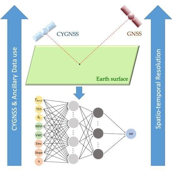
:This paper presents a learning-based, physics-aware soil moisture (SM) retrieval algorithm for NASA’s Cyclone Global Navigation Satellite System (CYGNSS) mission. The goal of the proposed novel method is to advance CYGNSS-based SM estimations, exploiting the spatio-temporal resolution of the GNSS reflectometry (GNSS-R) signals to its highest potential within a machine learning framework. The methodology employs a fully connected Artificial Neural Network (ANN) regression model to perform SM predictions through learning the nonlinear relations of SM and other land geophysical parameters to the CYGNSS observables. In situ SM measurements from several International SM Network (ISMN) sites are used as reference labels; CYGNSS incidence angles, derived reflectivity and trailing edge slope (TES) values, as well as ancillary data, are exploited as input features for training and validation of the ANN model. In particular, the utilized ancillary data consist of normalized difference vegetation index (NDVI), vegetation water content (VWC), terrain elevation, terrain slope, and h-parameter (surface roughness). Land cover classification and inland water body masks are also used for the intermediate derivations and quality control purposes. The proposed algorithm assumes uniform SM over a 0.0833 0.0833 (approximately 9 km × 9 km around the equator) lat/lon grid for any CYGNSS observation that falls within this window. The proposed technique is capable of generating sub-daily and high-resolution SM predictions as it does not rely on time-series or spatial averaging of the CYGNSS observations. Once trained on the data from ISMN sites, the model is independent from other SM sources for retrieval. The estimation results obtained over unseen test data are promising: SM predictions with an unbiased root mean squared error of 0.0544 cm/cm and Pearson correlation coefficient of 0.9009 are reported for 2017 and 2018.
1. Introduction
Soil moisture (SM) has an active role in the Earth’s water cycle between the ground and the air. This role makes SM a key land geophysical parameter for understanding hydrologic processes, vegetation states, and climatic conditions in order to improve applications such as hydrologic modeling, agriculture, crop yield estimation and vegetation change detection, as well as weather and climate forecasts [1,2,3]. Global SM retrieval at high spatio-temporal resolutions, therefore, has been an important research topic for the past several decades.
The current state of the science for global SM estimation relies on microwave remote sensing with the use of traditional instruments such as monostatic radars and radiometers. This is because the microwave frequencies are sensitive to the changes in the soil dielectric properties with respect to the presence of moisture content [4]. In particular, L-band radiometry is commonly used because it has an increased sensitivity to the near-surface SM (0–5 cm) as well as its reduced attenuation due to the atmospheric losses, surface roughness, and vegetation cover [5]. ESA’s Soil Moisture and Ocean Salinity (SMOS) [6] and NASA’s Soil Moisture Active Passive (SMAP) [7] satellites are current missions that have on-board L-band radiometers and provide SM retrievals with a spatial resolution of around 40 km and revisit time of 2–3 days. On the other hand, radar backscattering generally offers finer spatial resolutions (tens of meters to few km) within longer revisit times except SMAP’s radar instrument (L-band), which was capable of providing a spatial resolution of 3 km and a revisit time of 2–3 days with the help of its rotating antenna before a hardware failure in mid 2015. SMAP mission was designed to make use of a 6 m mesh reflector antenna for both radar and radiometer instruments to provide high spatio-temporal resolution SM products [7,8]. In addition, the radar backscattering data of ESA’s Sentinel-1 (C-band) [9] and DLR’s TERRASAR-X (X-band) [10] were used for global SM estimates.
Global Navigation Satellite System Reflectometry (GNSS-R) is an alternative microwave remote sensing approach, which is based on reception of the reflected GNSS signals from the Earth surface in a bistatic geometry [11]. This approach shows a great potential for remote sensing of SM because it operates at L-band. Moreover, it can offer high spatial resolutions with low revisit times by using constellations of small satellites due to being strictly “receive-only” [12]. GNSS-R applications have seen advancements for various Earth science areas over the past two decades that have resulted in the launch of new satellite missions [13,14,15,16]. For instance, the first dedicated spaceborne GNSS-R receiver was a secondary payload on-board the UK Disaster Monitoring Constellation (DMC) [17]. It has demonstrated the potentiality of GNSS-R for the remote sensing of ocean, ice, and land geophysical parameters [18]. The UK Technology Demonstration Satellite (TDS-1) was launched in 2014 with an improved primary GNSS-R payload, Space GNSS Receiver-Remote Sensing Instrument (SGR-ReSI), which provided more data that were used to study GNSS-R sensitivity to SM [19,20]. NASA’s Cyclone GNSS (CYGNSS) was launched in December 2016 to improve weather predictions by estimating ocean winds between 38 north and 38 south latitudes [21]. CYGNSS has eight small satellites in orbit, each with four channels, allowing simultaneous measurements from up to 32 channels. It has a mean revisit time of seven hours over the ocean. The key orbital and instrumental specifications of the CYGNSS mission are listed in Table 1. The constellation records a considerable amount of land observation data as well. CYGNSS measurement sensitivity to the surface SM has been reported by multiple studies [12,22,23,24]. These efforts demonstrated GNSS-R’s potential to complement the traditional passive and active instruments for monitoring surface SM at global scales for improved spatio-temporal resolutions.
CYGNSS is not designed for land observations; however, a CYGNSS-based, accurate SM retrieval algorithm could enable scientists (i) to specify the requirements for dedicated SM missions of the future, (ii) to create new algorithms utilizing existing land data, and (iii) to discover new calibration/validation approaches for dedicated GNSS-R SM missions. Motivated by this, there have been increasing efforts to develop SM retrieval algorithms for CYGNSS observations. For example, Chew and Small [22] correlated the changes in the CYGNSS signal-to-noise ratio (SNR) with the SMAP SM estimations, assuming that CYGNSS land measurements are dominated by the coherent reflections. They used mean SMAP SM values as reference with these correlations to obtain daily, CYGNSS-based SM estimations from SNR changes for each SMAP Equal-Area Scalable Earth (EASE) grid (36 km × 36 km) [26]. The overall unbiased root-mean-squared error (ubRMSE) of their algorithm is 0.0450 cm/cm. Although the estimation method itself relied on SMAP SM data as a reference, its significant benefit was that linking CYGNSS SNR to SMAP SM products allowed the use of CYGNSS observations to fill in the gaps between the adjacent SMAP observations. Kim and Lakshmi [27] introduced a relative SNR (rSNR) and SM derivation from CYGNSS delay-Doppler maps (DDM) to infill the gap between adjacent SMAP revisits. They reprojected the CYGNSS SNR observations into SMAP’s 9-km EASE grids and calculated the average of these grids to acquire daily SM estimations. They combined rSNR with SMAP SM values to acquire daily SM estimations over high vegetation density as well. They reported correlation results at useful levels (Pearson R of 0.77 between CYGNSS-derived SM and SMAP) over moderate vegetation density but with reduced correlations (R = 0.68) over dense vegetation; however, they did not report any error level (such as ubRMSE). Carreno-Luengo et al. [23] did not propose a CYGNSS-based SM estimation method; however, they made use of an approximated CYGNSS reflectivity, which is the ratio of the calibrated reflected and direct SNR measurements, assuming predominant coherent reflections over land. They linked CYGNSS reflectivity approximation to the SM changes for several land cover types. Clarizia et al. [28] introduced the trilinear regression-based reflectivity–vegetation–roughness (R–V–R) algorithm that derives daily SM estimations at a 36 km × 36 km resolution as a function of the CYGNSS reflectivity as well as SMAP vegetation opacity and roughness coefficient. The algorithm was developed considering the dominance of the coherent reflections over land. The R–V–R performance was compared globally to the SMAP SM product and reported to have a RMSE of 0.07 cm/cm. Al-Khaldi et al. [24] proposed a time-series SM retrieval algorithm that produces 3-day and 1-day SM estimates. In contrast to former studies, they assumed that the CYGNSS land returns are mostly driven by the incoherent scattering unless inland water bodies exist within the footprint. Therefore, they used the CYGNSS normalized bistatic radar cross section (NBRCS) and mean-square slope (MSS) instead of the DDM SNR. As a result, they provided SM estimations at relatively coarse resolutions (0.20.2 lat/lon grid roughly 22 km around the equator) with an overall RMSE of 0.04 cm/cm. They constructed a system of equations for 30-day time-series of the CYGNSS measurements, which is indeed an under-determined system with 29 equations. Hence, they incorporated the SMAP maximum and minimum SM values into the algorithm for bounding the system. They also assumed that changes in vegetation and surface roughness occur much slower compared to changes in SM.
This paper proposes a physics-aware machine learning approach through capturing the nonlinear dependencies of the CYGNSS observables to SM values and several bio/geophysical parameters that represent vegetation and ground effects. An Artificial Neural Network (ANN) is employed to learn the complex nonlinear relations. The term “physics-aware” in this manuscript refers to the use of several ancillary data sets and International Soil Moisture Network (ISMN) measurements to represent the vegetation and ground dynamics in the learning process. The details of the data usage will be explained in the next section. Daily SM measurements are used both in training of the model and validation of the SM predictions. One of the main objectives of this study is to initiate a novel, practically applicable SM retrieval algorithm that can provide sub-daily SM products within a few kilometers by utilizing the individual CYGNSS observations as the algorithm inputs. Once trained on a reference data set, this method neither requires SM information from other satellite missions, nor operates on spatial or temporal averaging of the CYGNSS observations. SM retrieval performances for multiple ISMN sites are visually and quantitatively demonstrated.
The rest of the paper is organized as follows: Section 2 describes the theoretical background of the GNSS-R based SM retrieval, possible use of CYGNSS data products, and the related challenges, followed by Section 3 with the explanation of the SM retrieval methodology, details of the ANN model, acquisition of the data sets, as well as training and validation. Section 4 provides the SM estimation results along with the visualizations and statistical performance metrics achieved. Section 5 gives a comprehensive discussion of the findings and points to be improved in the future. Section 6 concludes the study.
2. Theoretical Background
Bistatic CYGNSS radars receive the L-band GNSS-R signals that are transmitted by the GPS satellites and subsequently forward-scattered from Earth’s surface in the specular direction. This configuration of the CYGNSS and GPS constellations functions as a bistatic radar at L-band, which receives information relevant to the scattering surface properties. SM can be retrieved as part of such information overland as it is the primary determinant of the dielectric constant of the scattering surface. This section provides theoretical background for SM retrieval from bistatic radar observations, potential use of CYGNSS observables in such a task, and related challenges.
2.1. Inversion of the Bistatic Radar Equations
An ideal GNSS-R based SM retrieval approach would rely on inversion of the bistatic radar equations to acquire the surface reflectivity. The surface reflectivity would be corrected for the vegetation cover and surface roughness effects to obtain a Fresnel reflection coefficient. Fresnel reflection coefficient could then be related to SM with the help of Fresnel reflection equations.
For cases where specular reflections are fully dominant, the coherent component of the bistatic received power can be written as follows [11,29,30,31]:
where denotes the coherently received power. The subscripts R and L stand for the right-hand circularly polarized (RHCP) GNSS transmit antenna and the LHCP downward-looking GNSS-R antenna, respectively [11]. is the free space wavelength, is the peak power of the transmitted GNSS signals, is the gain of the transmitter antenna, is the gain of the receiver antenna. is the distance between the specular reflection point and the GNSS transmitter, while is the distance between the specular reflection point and the GNSS-R receiver. denotes the specular reflectivity at a local incidence angle of .
The incoherent component of the bistatic received power can be written as follows [32,33]:
where denotes the bistatic received power due to the the diffuse scattering over the surface. is the bistatic radar cross section (BRCS) in m. BRCS can be further defined as follows:
where the quantity is the contributing surface area (frequently called the glistening zone [11]), from where the diffuse scattering originates. is the normalized BRCS (NBRCS), which includes the spreading loss and the path-dependent phase terms for diffuse mechanisms (such as single scattering or multi-scattering) in the various multi-path directions for the scattering particles (mainly due to the vegetation canopy) and the surfaces (topography and roughness) [31].
The bistatic received signals are assumed to be dominated by the coherent reflections when the surface is relatively flat (no topographic relief) and smooth (weak roughness), having no or non-heavy vegetation cover [11,12,22,28,34]. The surface reflectivity in this case can be obtained by directly solving (1) for , as shown below:
Furthermore, it can also be computed by substituting Equation (1) into Equation (2) with (i.e., equating the right-hand-sides of two equations to each other) and obtaining as a function of [35] as follows:
Above calculation (correction for the path loss and the term) functions as a correction to for coherency assumption, whereas is originally computed assuming incoherency.
After obtaining the surface reflectivity, , by using either (4) or (5), the Fresnel reflection coefficient, , should be derived from for SM retrieval. This is because is mainly driven by the moisture content of the soil (SM) [4]. can be calculated by correcting for the vegetation [36] and surface roughness effects assuming the rough surface under the vegetation to be flat and smooth and to follow Kirchhoff’s approximation with a Gaussian height distribution [37] as follows:
where the exponential term in (6) accounts for the surface roughness effects. The h-parameter is assumed linearly related to the root-mean-square-height surface roughness [38], as follows:
where is the angular wavenumber and s is the surface root-mean-squared (rms) height.
The squared transmissivity, , in (6) accounts for the wave attenuation as the waves propagate from the top of the vegetation canopy to the ground and then from the ground to the top of the vegetation cover again. The transmissivity depends on the vegetation optical depth, , and the incidence angle as follows:
and (and parameter b in (9)) are dependent on the electromagnetic signals’ polarization, but the polarization notation is waived here for simplicity. The vegetation optical depth has been previously related to vegetation water content (VWC) and a land cover-based proportionality value (b) that depends on both the vegetation structure and the microwave frequency in the literature [36], and this approach has been successfully applied to the coarse spatial resolution SMOS/SMAP missions [6,7], as shown below:
VWC was empirically derived from normalized difference vegetation index (NDVI) by the SMAP mission with additional utilization of the minimum and maximum NDVI values of ten-year time-series, and the stem factor parameter that comes from a land cover-based lookup table (LUT) [39] as follows:
Equation (6) could be solved for the Fresnel reflection coefficient, , substituting equations from (6) to (10). It could then be related to the soil dielectric constant, , with the help of the Fresnel reflection equations as follows:
where
The soil dielectric constant, , can be related to SM with the help of a ground dielectric mixing model by using soil texture information. A number of dielectric mixing models has been developed in the literature such as Dobson [4], Mironov [40], or Wang–Schmugge [41] models. It should be noted that some of these models might require the use of additional geophysical parameters such as soil temperature [40].
2.2. Potential Use of CYGNSS Data
CYGNSS receivers process delay-Doppler maps (DDM) as the main observatory product [11]. CYGNSS Level 1 v2.1 Science Data Products, definitions of which can be found in Appendix A, include a number of geometry- and instrument-related DDM-derived variables.
With respect to the consideration of the dominant coherent reflections described previously, the surface reflectivity can be approximated by using either (4) or (5) with the CYGNSS data products. For instance, the CYGNSS data can be substituted into the calibration parameters in either equation as follows: for , for , for , for , and for . In order to perform the calculation by using (4), the bistatic received power, , needs to be substituted by a CYGNSS observation. Using either or the peak of the DDM was investigated by previous studies [22,23,27,28,35]. The product accounts for the peak DDM signal-to-noise ratio (SNR) and is computed as , where is the maximum value (in raw counts) in a single DDM bin and is the average raw noise counts per bin [33].
To solve (5) for the surface reflectivity, data product (Appendix A) of the CYGNSS mission can be used. In principle, this should produce an output equal to the use of peak power in (4); however, the resulting reflectivity approximations have differences from each other, which is most likely due to the internal calibration process when generating . Although the CYGNSS data products are originally calibrated for ocean surface sensing, using over land is valid since it is only calibrated for the instrumental and geometric parameters [35]. is published as a DDM within the CYGNSS Level 1 data; however, the peak value can be exploited under the coherency assumption. The rest of the derivation through (5) is based on the calibrations with respect to the range terms.
2.3. Challenges
Despite the potential usability of the CYGNSS data products in the reflectivity calculations through (4) or (5), the uncertainties in the determination of these data products in the present Level 1 data version (v2.1) would introduce errors in the estimations. Uncertainties in the current CYGNSS data include estimation of the receiver gain as well as the GPS transmitted power and gain. Furthermore, the transmitter and the receiver ranges to the specular point (SP) might involve errors since the current SP calculation of the CYGNSS mission uses an ellipsoidal model of the Earth, ignoring topography over land [28,42]. Since the equations from (4) to (11) can only provide the optimal solution with the computation of an absolute reflectivity, such errors would require subsequent corrections for accurate SM retrieval.
Additionally, varying land covers (especially, mixtures of heavy vegetation canopies such as forests) and topographic relief over land can introduce an ambiguity about where and under what conditions the coherent reflection regime is dominant. When the incoherent component of the bistatic received power superimposes or dominates the coherent reflections, the use of (4) and (5) would lead to inaccuracies.
In addition to the aforementioned challenges so far, the SM retrieval process itself contains high complexity and nonlinearity. This is because Equations (4) through (11) imply that the retrieval problem is dependent not only on the reflectivity and SM but also on the vegetation, surface roughness, topography, and soil texture through a combination of linear and nonlinear relations. Moreover, these land geophysical parameters have distinct variability ranges. In addition, the CYGNSS DDM instrument (DDMI) has diverse sensitivities to these parameters [43]. As a result, CYGNSS observations exhibit nonlinear relations with the dynamic land parameters. This leads to parameter ambiguity, where varying combinations of multiple land geophysical parameters might result in the same or close sensor measurements. Parameter ambiguity makes the SM retrieval an ill-posed problem. Additionally, to obtain accurate retrieval results, the impact of the measurement geometry (incidence angle) as well as the internal and external noise need to be properly accounted for. Previous airborne GNSS-R experiments and modeling studies reported supporting observations and simulated results for these effects, where a dynamic range of roughly 15 dB is determined jointly by the several dynamic geophysical parameters throughout crop seasons [34,44].
The CYGNSS constellation has sub-daily, quasi-random observations with fine spatial resolutions. Despite the advantage due to high spatio-temporal resolution, this complicates the use of ancillary data for accurate representation of the land geophysical parameters. In other words, finding sufficiently accurate input parameters at the high spatio-temporal resolutions of the CYGNSS observations to correct the vegetation and surface roughness effects as well as solving the Fresnel reflection equations are a concern. It is evident from Equations (4)–(11) that knowledge of the various parameters from vegetation and surface roughness to soil texture is needed at CYGNSS’s resolution for accurate retrieval using the given physical model for the coherent reflection assumption. In fact, simplified LUTs (such as land cover-based or globally constant values) or average values per coarse grids were used to approximate these parameters in the coarse spatial resolution SM retrieval missions such as SMOS [45] and SMAP [38]. The reduced sensitivity of the radiometers to the roughness and vegetation makes this possible for the relatively coarse observations of these missions. Nonetheless, CYGNSS provides quite fine spatial resolutions (from hundreds of meters to several kilometers, depending on the coherence, incidence angle, elevation, and orientation) with frequent revisit times (several hours to few days), and its measurements are highly sensitive to the topography, surface roughness, and vegetation changes [23]. Thus, even successive observations along the CYGNSS track can have largely different values due to the spatial variations in these land geophysical parameters. Figure 1 illustrates this phenomenon by inspecting the CYGNSS observations after the Hurricane Florence landfall on North Carolina, USA. It shows the mean of the uncalibrated CYGNSS SNR values from 14–18 September 2018 that are averaged per SMAP grid pixels (roughly 36 km × 36 km). The zoomed-in version of one of the grids demonstrates the actual CYGNSS data where spatial and temporal variability of the CYGNSS measurements even within a SMAP pixel is apparent. It is evident from Figure 1 that the CYGNSS mission, or GNSS-R in general, offers a sufficiently high spatio-temporal resolution which can help improve hydrological and agricultural applications. Therefore, the detailed information from this resolution gets lost due to any spatial gridding and/or temporal averaging while developing a CYGNSS-based SM retrieval methodology. For instance, previous SM retrieval attempts gridded multiple CYGNSS data points into larger grids (such as 36 km × 36 km SMAP EASE-grid) even though the coherent reflections over land are considered [22,28].
Regarding the methodological challenges and the retrieval complexities described so far, regression techniques can be practical for the CYGNSS-based SM retrieval problem instead of pure explicit solution of the physical model shown in Section 2. In principle, such techniques are based on fitting a regression model between the known SM values from a reference data set (such as SMAP, SMOS, or in situ SM networks) and the CYGNSS observations (possibly in conjunction with ancillary data), and exploiting this model to perform future SM estimations. There have been previous efforts conducted to obtain variations of linear regression models [22,28]. As Clarizia et al. [28] state, however, linear regression approaches may be too simplistic to deal with the nonlinear dependence of the CYGNSS observations on SM and the other land geophysical parameters (SM, vegetation canopy, topography, surface roughness, and soil texture). For instance, large local variations between NDVI and topography occur at very high resolutions (few tens of meters) [46]. Such a high spatial variation of parameter correlations, combined with diverse sensitivity of CYGNSS DDMI to different parameters, would make linear regression approaches perform poorly.
3. Soil Moisture Retrieval Methodology
We have developed a new, CYGNSS-based SM retrieval methodology that exploits a non-parametric, nonlinear machine learning (ML) technique, namely ANN. The decision to use this method is motivated by its following properties and correspondences to the aforementioned requirements as well as challenges of the SM retrieval from CYGNSS observations:
- Nonlinear ML algorithms are known for their solid power to solve regression problems where a mix of linear and nonlinear dependences exists between parameters [47].
- Such techniques, ANNs in particular, are capable of approximating/learning complex mappings within multi-dimensional parameter spaces with the help of advanced learning algorithms.
- ANNs can, in principle, be trained to approximate any measurable function to any desired degree of accuracy to represent arbitrary input–output relations [48]. It should not turn out that the methodology in this study relies on such arbitrary relations. On the contrary, the CYGNSS observables and ancillary data that are major inputs to the regression process are used in order to fulfill the linear/nonlinear relations as well as calibration/correction requirements shown in Section 2. The property of ANNs makes the use of proxy input features possible for the purpose of fine-tuning the overall model performance.
- ANNs are non-parametric models, meaning that the number of parameters that can be input to the retrieval process is flexible, in contrast to the requirement for fixed number of parameters in the parametric models (such as traditional regression models, physical and/or empirical models). This can help advance the CYGNSS-based SM retrieval approaches by introducing the use of additional parameters into the retrieval process. For instance, the CYGNSS trailing-edge slope (TES) can be input into the SM retrieval as a coherency/incoherency indicator in addition to reflectivity, as previously practiced for a study of inundation detection by using another non-parametric learning method [35], instead of dealing with the explicit determination of the coherency.
- The non-parametric nature of ANNs make these models applicable to learn many different kinds of data regardless of their statistical properties. In other words, the retrieval process can integrate data coming from different sources with even poorly-defined (or unknown) probability distributions and relate them well to the parameter of interest [47]. To illustrate, LUT-based SMAP data such as h-parameter (roughness parameter) and stem factor [39] can be incorporated into the CYGNSS SM estimates, combining with in situ data such as land cover and NDVI.
- Consequently, such models have to make fewer assumptions about the data distribution, compared to the parametric models. This should not, in turn, mean that the parameters of the CYGNSS-based SM retrieval process have poorly-defined probability distributions. In contrast, it will be demonstrated throughout this section that most of the input parameters coming from CYGNSS observations and ancillary data exhibit well-defined distributions. However, it is a powerful flexibility for ancillary data usage that there is no need to make any assumption about the data distributions.
- The use of such learning algorithms eliminates the need for development of a parametric model that is aimed at explicitly solving the electromagnetic relations and/or relating the in situ observations to sensor measurements. This could be beneficial for the SM retrieval from CYGNSS observations to overcome the aforementioned limitations of ancillary data and possibility of too simplistic assumptions.
- ANNs are generally said to be a good balance between accuracy, stability, and computational speed [9].
Throughout this section, insights into the ANN model architecture will be provided first, then detailed information about the data sets that are used in this study will be given, and, finally, how the data sets are used in the learning process (training and validation) will be explained.
3.1. ANN Model Architecture
In this study, we employ a fully-connected ANN architecture, also known as Multilayer Perceptron (MLP), for the nonlinear regression problem, as shown in Figure 2. Input features to the learning process are the surface reflectivity, TES, and SP incidence angle from the CYGNSS observations; NDVI and NDVI-derived VWC from MODIS Aqua Surface Reflectance Daily Global 500m data set [49] to represent the vegetation canopy; elevation, terrain slope, and h-parameter values from the CGIAR-CSI SRTM 90m, Version 4 digital elevation model (DEM) database [50] to stand for the surface dynamics. The selection of these input features were determined after a number investigations on their individual and combined contributions to the estimation performance. The results of these investigations will be provided in Section 4 (see Table 4). The acquisition of the input features from CYGNSS and ancillary data sets as well as the SM data will be comprehensively explained later in this section.
Reference SM data (in the output layer) are used for optimization of the ANN parameters (minimization of the loss function) in the training stage and assessing the model performance in the validation phase. The proposed model minimizes the loss function, which is defined as the squared error between the model-calculated SM and the reference SM values, over the training data set by running over a predetermined number of iterations. ANN parameters are learned through a stochastic gradient descent solver algorithm, where, within each ANN iteration, the model parameters are updated by computing the partial derivatives of the loss function with respect to the ANN parameters (back-propagation) [51,52]. In other words, the model learns in the training phase the nonlinear dependences between the CYGNSS measurements and the reference SM labels with the corresponding ancillary data. Then, the trained model uses these dependences to make future SM estimations for a given set of CYGNSS observations and ancillary data.
In fully-connected ANNs, neurons of one layer are fully interconnected to each other neuron of the adjacent layer. Each layer has a weights-array that can be trained by the forward and backward propagation mechanisms. This array controls the linear strength of the connections to the next layer [51]. Assuming that the number of neurons in ith layer is , the weights-array at the ith layer has a size of ( × ). The inputs-array has a size of (8 × M), where 8 is the number of inputs and M is the number of data samples. The result of the matrix multiplication between weights-array and inputs-array of a particular layer is given as input to the next layer. To account for bias in such a linear relation, a trainable bias value is added to the sum at each neuron. The process described so far defines no more than a linear relation in each neuron, and, if it was the only operation for the entire ANN, it would only result in a linear regression. The essential part of ANNs that make them powerful to solve nonlinear regression problems is the activation function for each neuron. In the literature, a number of different activation functions are used such as Rectified Linear Unit (ReLU), logistic, or tanh activations [53,54]. These functions are responsible for taking the corresponding bias-added sum as input and transferring it to a new value with the help of the corresponding nonlinear relation. This process at each neuron is repeated until the output layer is evaluated, which gives the predicted SM value in this study. The calculation from inputs to the output is named forward propagation. The network uses the training data and back-propagates the error information by updating the weights and bias in each layer [51] to minimize the defined loss function with the help of a stochastic gradient descent algorithm. The entire process makes one iteration of forward and backward propagation. Such iterations are made until the loss function reaches a threshold minimum value or a maximum number of iterations are performed. After the described learning process is finished, the final set of node weights and biases for each layer builds up the trained ANN model for SM predictions. This learned network will produce SM estimates from any new input data parameters through a single forward propagation.
We have tested several ANN structures, and the ANN parameters that give the best performance out of our investigations are as follows: The input layer has the same number of nodes as the number of used features, which is 8. The output layer has a single node which is the predicted SM values. ANN has two hidden layers in addition to the input and output layers, as shown in Figure 2. The nonlinear activation function at each layer is chosen to be the Rectified Linear Unit (ReLU) function [53] as it gives the best overall results compared to logistic or tanh activation functions [54]. The last layer is only a regression layer with no activation function. The Adam solver, which is a first-order gradient-based optimizer for stochastic objective functions [55], is employed for solving optimal weights through loss-function minimization with a learning rate of 0.0001.
3.2. Data Sets
This subsection provides details about the acquisition of the SM, CYGNSS, and ancillary data sets as well as their expected contribution to the regression, and the quality control steps to eliminate erroneous data from the analysis.
3.2.1. Reference Soil Moisture Data
The present study uses daily SM measurements from in situ ISMN sites as reference for the training and validation. The decision to use these data instead of other global SM sources (such as SMAP/SMOS) is built upon three main reasons: (i) comparisons can be made better in a daily basis, compared to 2–3 day revisit time of SMAP and SMOS missions. (ii) This study is conducted to investigate high spatial resolution CYGNSS-based SM estimates; however, comparisons with missions like SMAP or SMOS would require the use of a resolution of roughly 36 km, which under-utilizes CYGNSS’s potential. (iii) If the learning is done using SMAP-like satellite observations, the performance of the learning process will be limited by the retrieval performance of that source. For this purpose, a 0.0833 0.0833 lat/lon grid (approximately 9 km × 9 km around the equator) centering each SM site is considered as a representativeness window where the SM measurements are assumed to be constant. Although this assumption may not always hold as SM can vary much across short distances, it is a necessary assumption in the current state-of-the-science. For instance, the use of SMAP or SMOS missions would require to assume a constant SM value over 36-km regions due to the resolution. Moreover, similar approaches were made in the literature; for example, Dorigo et al. [56] assumed a coarse 50-km window around the ISMN sites. Hereafter, the SM representativeness window around SM sites will be called a 9-km grid in the manuscript.
SM data from 18 ISMN sites throughout North America and Australia are analyzed, considering that there are a sufficient number of data samples (CYGNSS observations, reference SM values, and corresponding ancillary data) to input to the ANN model as well as there being enough variability within each parameter (see Figure 6). Fifteen ISMN stations are chosen from Soil Climate Analysis Network (SCAN) sites from the United States of America [57], and the remaining three are from an OzNet Hydrological Monitoring Network site from Australia [58]. Detailed information about these SM sites are given in Table 2. The locations and International Geosphere-Biosphere Programme (IGBP) land cover types of these ISMN sites are shown in Figure 3, which is visualized by using the MODIS/Terra + Aqua Land Cover Type L3 Yearly Global 500 m V006 data set [59] via Google Earth Engine Python API [60]. The selection of these ISMN sites are based on the following reasons: (i) The latitudinal coverage of CYGNSS (38 north and 38 south) limits the use of several networks; for example, no station from Europe can be included in this study. (ii) Because GNSS-R is sensitive only to the top 5 cm of the soil, the ISMN sites that measure SM at this depth are considered comparable to the CYGNSS estimations [56]. For instance, the COSMOS network would be an alternative network, but their measurements are taken from a varying interval of 0–39 cm. (iii) The uniformity of the sensor technology is another constraint. Despite the internal uncertainty of each SM probe, choosing SM networks of the same SM measurement technology would avoid additional biases between the networks. SCAN and OzNet sites are chosen because most of the stations of both networks employ the same instrument (Stevens Water Inc., Hydraprobe). (iv) The diversity and temporal coverage of the published data by the networks is also significant as the present analysis needs annual SM data for 2017 and 2018 as well as the temperature measurements for a quality control. For example, the PBO_H2O network was not included in the analysis because their sites provide SM only (Additionally, their measurements are not based on a physical SM probe; instead, their sites are examples of GNSS interferometric reflectometry based SM estimation). (v) Most of the ISMN sites in the data set are located on relatively flat (non-mountaneous) surfaces with low-to-moderate vegetation cover (such as croplands, grasslands, savannas) for the sake of limiting the incoherent scattering effects in the analysis.
The SCAN sites provide daily mean SM (measured from top 2.5–5 cm of the soil), air temperature, and precipitation measurements for annual periods. The OzNet sites provide 20-min SM (for top 0–5 cm of the soil), soil temperature (measured at top 2.5 cm), and precipitation measurements for annual periods. Therefore, their measurements are preprocessed in order to obtain daily averages in this study. Measurements from years 2017 and 2018 for both SCAN and OzNet networks are used in this study since CYGNSS measurements have been made available starting from mid-March, 2017.
3.2.2. CYGNSS Data
The CYGNSS observations with a SP location that fall into the 9-km grid of any of the ISMN sites throughout 2017 and 2018 are included in the analysis. We used the CYGNSS Level 1 v2.1 Science Data Products to obtain the following observables as CYGNSS-representative inputs to the SM retrieval algorithm: (i) Reflectivity, (ii) SP incidence angle, (iii) TES. The definition and acquisition of each input feature are as follows:
Reflectivity is the primary CYGNSS deliverable that must be input to the regression since it is the GNSS-R receivers’ observation of the changing SM values and surface conditions. The surface reflectivity can be derived from the CYGNSS data products by several methods as described previously in this manuscript and performed by other studies. Four different derivations were investigated in this study: (i) we calculated an approximate reflectivity by substituting the DDM SNR () into in (4) and calibrating for the instrumental and geometric parameters, as done previously [22,28]. This calculation is called in this manuscript. (ii) is generated similarly to the former approach except that the peak value of the analog power DDM () instead of DDM SNR is used for . For cases where error level in the DDM noise floor is high (DDM SNR and in turn would get erroneous), could provide increased correspondence to SM. (iii) is used to calculate the reflectivity as shown in (5), correcting the incoherency assumption by applying the coherent equation as well as compensating the path loss and term; this reflectivity is called [35]. (iv) was derived by using the ratio of the reflected and direct SNRs ( and , respectively), which are first calibrated by the range terms, as previously practiced [23]. Separate and combined effects of these reflectivity calculations were investigated in the SM retrieval, and the results reported in Section 4 demonstrate that alone has given the highest learning performance. This can be attributed to diverse levels of errors coming from changing calibration parameters in different reflectivity calculations. Therefore, the term “reflectivity” will, hereafter, be used for , unless otherwise stated.
SP incidence angle (in degrees) is used as given in the CYGNSS data. Incidence angle should be taken into account in the CYGNSS-based SM retrieval methods because of two reasons: (i) CYGNSS observes the Earth surface over a wide range of incidence angles spanning from 0 to 70 with a mean of approximately 30 and a standard deviation of roughly 17, (ii) Observed reflectivity values are dependent on the SP incidence angle [24]. Calibrating the reflectivity values for changing incidence angles can be done by two techniques: (i) Normalize the reflectivity values at any angles to their corresponding level at 0 by using a curve fit function, (ii) Input the incidence angle as a feature to the learning model and let the model capture the angle dependent curve fit for the reflectivity values. We examined both of these approaches, implementing the former by applying as Al-Khaldi et al. considered [24]. Statistical results of the investigation are demonstrated in Section 4; however, using the SP incidence angle as an input feature to the ANN model (latter approach) worked slightly better. We attribute the weaker performance of the former to the fact that the curve fit function is based on empirical observations for typical loam soil parameters, which may not be the case for all the ISMN sites in our analysis.
TES is computed as the slope of the trailing edge of the reflectivity delay waveform, as defined by Rodriguez-Alvarez et al. [35]. TES calculation is dependent on the shape of the CYGNSS DDMs and is, therefore, directly related to the coherency/incoherency of the GNSS-R signals. More incoherent mixing through the scattering surface makes TES smaller [35]. Even though this study assumes the dominance of the coherent reflections, we consider the inclusion of TES in the SM retrieval method to be useful for feeding the regression with a coherency/incoherency metric.
3.2.3. Ancillary Data
The use of ancillary data as input to the retrieval process is required since the GNSS-R reflectivity is sensitive to not only SM but also other geophysical parameters such as vegetation canopy, topography, surface roughness, and soil texture. It should also be noted that the calculated reflectivity involves the effects from these parameters and are not corrected prior to the retrieval in this study. We used several data sets to represent these parameters as the following input features to the learning model: (i) NDVI, (ii) VWC, (iii) Elevation, (iv) Slope, and (v) h-parameter (Roughness parameter). These input features are computed for every CYGNSS data sample in the analysis and given as input to ANN with the corresponding CYGNSS observables and SM value.
Before getting insight into the ancillary data acquisition, the spatial resolution of this algorithm should be explained. As defined in [35], the semi-major and semi-minor axes of the first Fresnel zone ellipse, where the coherent signals come from, varies between 0.6 km and 0.9 km, as well as 0.6 km and 2.3 km, respectively, for a change of SP incidence angle from 0 to 65. Depending on the relative orientation of the CYGNSS spacecrafts and GPS transmitters, the first Fresnel zone gets a varying orientation with respect to the along-track direction of the CYGNSS receivers as well. The distance traveled by the SP during the incoherent integration of the GNSS-R signals for one second is roughly 6 km, and it adds an elongation effect to the first Fresnel zone along track direction. In the marginal case where either (i) the semi-major, or (ii) semi-minor axis aligns with the along-track direction, such an elongation would only affect that axis. As a result, the final size of the CYGNSS footprint, which can no longer be an ellipse after the elongation, should, in marginal case (i), vary between 6.6 km and 8.3 km in the along-track direction, whereas the cross-track direction would only vary from 0.6 km to 0.9 km, depending on the incidence angle variations. Therefore, the spatial resolution of CYGNSS would vary between 0.6 km × 6.6 km and 0.9 km × 8.3 km. Similarly, in the marginal case (ii), the spatial resolution of CYGNSS would vary between 0.6 km × 6.6 km and 2.3 km × 6.9 km. All other possibilities of the footprint orientation on the surface would result in a spatial resolution in between the minimum and maximum of these marginal cases. On the other hand, computations of the Fresnel zone ellipse would have errors depending on the elevation because of the current SP calculation method of CYGNSS that considers Earth as an ellipsoid without topography [28]. Based on these data facts, we considered that a 0.04 0.04 (approximately 4 km × 4 km) lat/lon grid cell that centers the SP could be capable of generating the mean terrain statistics (elevation, slope, NDVI, etc.), which, in turn, was assumed to correspond to the CYGNSS footprint of interest and define the geophysical conditions around the SP location. This grid cell makes an approximate 4 km spatial resolution for SM retrieval since each CYGNSS observation in the analysis is used separately to generate a SM value. Hence, this grid will be called a 4-km grid from now throughout the manuscript. Figure 4 shows an example of such grids from the analyzed data set. The descriptions of the NDVI, IGBP land cover classifications, elevation and slope, and inland water body data sets will be given later in this section.
NDVI represents the vegetation cover above the ground as it was previously exploited by the SM missions [6,38]. Although by definition NDVI ranges from −1 to 1, normally, it is positive, and getting values closer to 0 or 1 for sparse or dense vegetation canopies, respectively. Two different, dynamic data sets were investigated for NDVI data throughout 2017 and 2018: (i) The NOAA Climate Data Record (CDR) of AVHRR Daily NDVI , Version 4 [62], (ii) MODIS Aqua Surface Reflectance Daily Global 500 m data set [49]. The latter has been chosen for its higher spatial resolution. NDVI is calculated from the near-infrared (NIR) and red bands (RED) of the reflectance data as . The mean NDVI for the 4-km grid of each CYGNSS observation is generated from the MODIS data with the following methodology: The data set is accessed via Google Earth Engine Python API [60] to rapidly and accurately perform analysis for multiple CYGNSS observations at a time. It is possible with the help of very high computing power of the Google Cloud Platform while benefiting the same interface for all different satellite data sets. NDVI data usually suffer from clouds because it is generated by optical instruments such as in the MODIS mission. To deal with this problem, we applied a sliding window averaging over 16 days, whose center is the day of interest (eight days ahead and seven days to the past). Noting that the 4-km grid houses spatial pixels, we have an NDVI cube for each day. To eliminate the ill (cloud-suffered or so) NDVI values, we only considered the width of two standard deviations of the distribution within the NDVI cube to calculate the mean NDVI for that particular grid and day of year [63]. Such an approach would produce close numerical values for adjacent days or short time-series; however, it is the representation of the reality rather than being a problem. More precisely, NDVI experiences quasi-constant trends in daily or weekly periods, and shows stronger dynamics through seasonal changes. Furthermore, spatial variations exist within the representativeness grid of each ISMN site mostly due to the mix of land covers. Land cover maps for the ISMN sites can be seen in Figure 5.
VWC is computed by using the NDVI data via Equation (10). To the authors’ knowledge, the accuracy of this empirical relation for high spatio-temporal CYGNSS resolution is not yet proven. Nevertheless, we decided to use VWC as an input feature in addition to NDVI since it encapsulates land cover information through stem factor and temporal memory information through minimum and maximum NDVI values. The stem factor information is a land cover-based LUT in the SMAP mission [39]. The stem factor value for the 4-km grid of each CYGNSS observation in this study is calculated as a weighted sum of LUT stem factors based on the land cover percentages in the scene. We performed two different VWC calculations: (i) and are computed from 2017 and 2018 NDVI data. (ii) The current NDVI is used in place of for the entire data set, and a global constant value of 0.1 was used for , as suggested in the SMAP’s VWC report [39] (Though suggestion for was for croplands and grasslands only). The former performed better in the SM retrieval, and we link this to the phenomenon that ISMN sites in this study were not only from croplands and grasslands as the latter method assumes.
Elevation and slope are used to assess their contribution to SM estimation as proxy parameters for the terrain topography, as topography is known to have impacts on the reflectivity [64]. The use of elevation is aimed at helping the regression model learn the impact of the ellipsoid-based CYGNSS SP calculation on the CYGNSS observations, if possible. The slope, on the other hand, is included in the input features as a coherency/incoherency indicator that could be linked to CYGNSS’s TES by ANN. Mean elevation and mean slope for each 4-km grid are generated from the static CGIAR-CSI SRTM 90 m, Version 4 DEM database [50], as similarly done in the literature [35]. DEMs of the ISMN sites can be seen in Figure 5.
The h-parameter is assumed to be linearly related to the root-mean-square-height surface roughness (7) [38]. Therefore, it is input to the SM retrieval in this study to assess its contribution to account for the surface roughness. h-parameter values are listed in a land cover-based LUT in the SMAP mission, similar to stem factor [39]. Therefore, we applied a similar calculation for h-parameter values over the 4-km grids as a sum of LUT h-parameter values that are weighted by the land cover percentages in the scene.
Distributions and corresponding statistics of the input features can be seen in Figure 6. These distributions were analyzed before and after the quality controls were applied. However, the distributions and statistics of the data after application of the quality controls did not drastically change. Since the quality controls are not yet described, only the statistics before the quality controls are given. Figure 6 shows that reflectivity follows an almost-perfect Gaussian distribution, so (one-sigma) of the reflectivity values fall in a dynamic range of around 10 dB, whereas (two-sigma) of them are in a dynamic range of roughly 20 dB. This is in parallel to the previously observed and simulated dynamic ranges of around 15 dB over cropland growth seasons [34,44]. Incidence angle follows a quasi-Gaussian distribution that reflects the variation of the CYGNSS observations, where of the measurements have an incidence angle in a range of approximately . The TES distribution is mostly around the mean value of −13.81 with few observations through larger negative values, which imply that the trailing edge of the reflectivity waveform from peak has a slope of −13.81 on average. The histogram of the elevation data shows the average elevation values around the ISMN sites. The slope distribution indicates that the regions generally have no topographic relief (majority of data under a terrain slope of 2), with a sufficient variation within a slope range of roughly [0.45, 2]. The h-parameter values show no more surprising evidence than that two peaks occur at the SMAP h-values of 0.108 and 0.156 that correspond to croplands and grasslands, respectively [38], and the rest of the data are distributed in between these values. NDVI data prove a good range of variation, where roughly of the NDVI values fall in an approximate range of [0, 0.58] since data seem to follow a nearly perfect Gaussian distribution. VWC distribution, as derived from NDVI by using stem factor values from the SMAP-based LUT, seems to be a mix of two Gaussian distributions around mean values (approximately 1.5 and 3.5 kg/m). These values likely correspond to grassland and cropland averages, which were the two most common land covers observed in this study.
3.2.4. Quality Controls
The quality control of the data sets plays a significant role in the preprocessing of the data for the SM retrieval. We made use of distinct quality control mechanisms for in situ SM measurements, CYGNSS observables, and ancillary data. The ideal impact of each quality control step is given Table 3, where percent changes in the original dat set is proved as if a particular quality flag is applied alone. In fact, the quality control flags were applied in the left-to-right order in Table 3.
Invalid SM values from the ISMN measurements (such as negative SM or precipitation value) are filtered out of the refrence SM data for both SCAN and OzNet networks. For SCAN sites, SM measurements that correspond to air temperatures below 1 C are excluded from the analysis due to the freezing conditions. The OzNet sites do not experience such conditions as the air temperatures in the region are far away from these ranges annually. CYGNSS observations and ancillary data are not collected for the dates that correspond to invalid and freezing-temperature SM data.
CYGNSS observations require further care to discard the low quality observations from the training and validation. We investigated two different sets of CYGNSS quality flags as Chew et al. [22] and Rodriguez-Alvarez et al. [35] previously applied and observed higher performance with the former. Despite a lack of sufficient investigation on the performances of these two quality flag sets, the weaker performance (ubRMSE = 0.0557) of the latter might be attributed to the reduced number of data samples used in the training (4027 samples after applying flags from [35]). The quality flags used to filter out the CYGNSS data in this study are as follows: S-band powered up, Large spacecraft attitude error, Black-body DDM, DDM is test pattern, Low confidence GPS EIRP estimate. CYGNSS measurements with a negative receiver gain estimation are discarded from the analysis. Table 3 shows the percent changes in the data set as if each of the quality flags was applied directly to the original data set. This approach helps demonstrate the true impact of each individual quality control to the data set. The negative receiver gain holds a reasonably big portion (26%) of the CYGNSS observations. Observations with a DDM peak value from outside the range (zero-delay corresponds to the 8th delay bin) are also removed to ensure the error in the CYGNSS SP location estimation due to the terrain elevation is within a reasonable range [22,35]. In addition, CYGNSS data points with an incidence angle above are removed due to the poor observation quality, similar to [24].
Inland water bodies have a critical impact on the SM retrieval process because GNSS-R signals get a step reflectivity waveform (sharp increase in the reflectivity) due to the very strong coherency over water surface [12,20,22,24,35]. Such impacts should be removed prior to the retrieval because they would not reflect SM effects in case the surface water is sufficiently large within the CYGNSS footprint. Being “sufficiently large” is commonly considered as even smaller than the first Fresnel zone [22,35]. Regarding the fact that the CYGNSS spatial resolution would range from a theoretical minimum of 0.6 km to 8.3 km depending on the incidence angles, and relative orientations of the instruments, we considered a size for the open water bodies that is close to the minimum resolution that would work to initiate investigations in this study. Hence, we removed the CYGNSS observations where more than one percent of the 4-km grid is covered by temporary (seasonal) or permanent surface water. We exploited the JRC Yearly Water Classification History, v1.0 data set (a.k.a. Pekel data set) [61], which is a 30 meter-resolution surface water database. Since the data set is only available from 1984 to the year 2015, we used 2015 data for this study. There are four values (0: No data, 1: Not water, 2: Seasonal-temporary water, 3: Permanent water) for any given pixel. We used the values 2 and 3 to perform water body removal, ignoring when or how long the seasonal water body existed in the year. It is evident from Table 3 that around 23% of the entire data set is excluded from the analysis due to inland water bodies. This effect is much higher for particular ISMN sites such as Sellers Lake (Florida, US), Fort Reno (Oklahoma, US), and Starkville (Mississippi, US). Inland water body maps of the ISMN sites can be seen in Figure 5.
3.3. Training and Validation
The SM measurement data are provided daily; however, the sub-daily availability of the CYGNSS observations for each ISMN site is not reduced to daily basis in this study. That is to say, for a particular day-of-year around one of the ISMN stations, if there are multiple CYGNSS SPs that fall into the 9-km grid that centers the site coordinates, all of them are included in the analysis. In such a case, a constant SM value is assumed for all of those multiple CYGNSS observations due to being in an ISMN proximity on the same day. This is considered feasible because the geophysical parameters (such as NDVI, VWC, elevation, slope, and h-value) corresponding to each CYGNSS observation would differ from each other due to the spatial variation, which in turn could explain variations in the CYGNSS observations despite uniform SM values.
After the quality control flags are applied, there are a total of 4808 reference samples (distinct feature vectors) from 18 ISMN stations, spanning from the 77th day-of-year of 2017 (starting date of the publicly available CYGNSS science mission data) to the end of 2018. The training and validation sets are organized with the help of a 10-fold cross validation fashion (N-fold in general [65]) as follows: training and validation are performed together in a total of 10 iterations. In each iteration, (i) of the total data samples are randomly selected and excluded from the training data; (ii) the ANN model is trained by using the data samples corresponding to the remaining of the data set; (iii) validation of the trained model is performed on the excluded data samples. By this method, the trained model is tested by using “unseen” data in every iteration. (iv) The predicted SM values are stored in the prediction pool with their corresponding reference SM values. (v) of the data excluded are turned back into the training data set. The next iteration is performed similarly to the following exception: The random selection of new of the data to be excluded for validation purposes is handled in a way such that samples in this validation set were never chosen into the validation set of any previous iteration. This regulation ensures that the training/validation split method validates the ANN model over the entire data set after 10 iterations are finished. (vi) When all 10 iterations are run, the prediction results for the entire data set with corresponding reference SM values are stored. (vii) Performance assessment of the entire data set is performed in order to obtain overall and per-ISMN-site statistical performance metrics such as RMSE, unbiased RMSE (ubRMSE), bias, and Pearson’s R (correlation coefficient) [66]. The overall training and validation approach is illustrated in Figure 7.
4. Results
Contributions of individual input features and their combinations to the learning process were first assessed in order to determine the optimal input feature set for SM retrieval. Table 4 shows the results of this assessment by using the indices from (i) to (xi) for changing input combinations. The bottom-most line provides the optimal set of input features that is employed in this study. (i), (ii), (iii), and (*) in Table 4 were conducted to compare CYGNSS reflectivity calculations, as shown in the top three rows and the bottom-most row. gives the highest correlation and lowest ubRMSE results. (iv) Then, a combination of these reflectivity approximations was assessed with two, three, or four of them being used together. All possible combinations were examined; however, only one of them with the closest performance () to the optimal one is given in Table 4. Although there is a slight difference between two, additional term reduces the overall performance of the optimal combination so that it is not included in the optimal combination. (v) Instead of giving the SP incidence angle as an input to the system, the reflectivity values are corrected for incidence and fed to the system without angle information; the model performance was slightly worse than feeding SP incidence angles to the learning. Hence, SP incidence angles were chosen into the optimal performance inputs set. (vi) Contribution of TES was examined and found to be significant as its removal increases the ubRMSE and decreases the correlation. TES is also chosen into the input features. (vii) and (viii) were performed to assess the effects of NDVI and VWC to the learning process. Both have a positive impact on the learning performances, but VWC has a more positive contribution compared to NDVI. This is in parallel with the expectation that VWC involves further information of temporal memory in and , as well as land cover information through . Both parameters are included into the input features. (ix), (x), (xi) were used to investigate the parameters that are derived from an SRTM DEM data set. All of them appear to positively affect the model, but elevation has the highest and h-parameter has the lowest impact on the overall performance. However, all of them are added to the input features set.
After the determination of the set of optimal input features, validation of the method with this set was performed. Figure 8 shows the scatter plots of the ISMN-measured and CYGNSS-retrieved SM values in conjunction with the RMSE, ubRMSE, bias, and Pearson’s R values for the entire data set, as well as years 2017 and 2018. In addition, per-site and overall performance statistics of the SM estimation results for the entire data set for both years are shown in Table 5. The entire data set, spanning both years, has a Pearson’s R value of 0.9009, which is an indicator of high overall agreement between the CYGNSS-based SM predictions and the reference SM data. Data over either year also show a high correspondence, with Pearson’s R values of 0.8532 and 0.9238 for year 2017 and 2018, respectively. These high levels of correlation demonstrate that the presented CYGNSS-based SM retrieval algorithm was successful in capturing the overall trends in approximately 5000 CYGNSS data samples. The ubRMSE values of 0.0575, 0.0520, and 0.0544 cm/cm for 2017, 2018, and entire data set, respectively, are obtained. Keeping in mind that both the science mission requirements for the SMAP mission over its calibration/validation sites were ubRMSE values no higher than 0.04 cm/cm [38] and CYGNSS land application studies were targeted at an ubRMSE of 0.05 cm/cm, our algorithm seems capable of generating close values to these levels at least for the current data set and input features of interest. It should be also noted here that, despite not being shown here, a previous version of this analysis was conducted with a subset of the data, input features, and quality controls; the overall performance (overall ubRMSE of 0.0594 cm/cm and Pearson’s R of 0.6604) was poorer than the ones reported here, although six of the ISMN sites with almost the best performances of this study were used. These observations are of high importance for the ultimate CYGNSS-based, or GNSS-R based in general, SM retrieval studies since the algorithm presented here has the potential to provide increased estimation performances as new satellite observation data and relevant input features are added to the training.
Considering the Pearson’s correlation coefficient ranges of [0, 0.3333), [0.3333, 0.6667), and [0.6667, 1] as low, moderate, or high correlations, of the stations have moderate as well as of them have high correlation results through 2017. For 2018, roughly of the sites have low, of them have moderate, and the remaining have high correlation levels. An interesting outcome of the correlation assessment is that, even though the highest Pearson’s R value for an ISMN site for 2017 is 0.8077 (Uvalde) and 2018 is 0.8909 (Uapb-Marianna), the overall Pearson’s R value for each year (0.8532 and 0.9238, respectively) exceeds these maxima. Moreover, the overall correlation coefficient for the entire data set (0.9009) is higher than these maxima as well. This is valuable especially for potential future application of the algorithm to the global scenarios, indicating that it is powerful to generalize the nonlinear regression for the entire data despite some poor performances on specific sites. Similar to the correlation, it can be reasonable to consider ubRMSE values above 0.0650 as low-performance, those in the range [0.0500, 0.0650] as moderate-performance, and values below 0.0500 as high-performance. In this case, the algorithm produces low-performance for of the sites, moderate-performance for , and high-performance for of those stations for 2017. For 2018, it predicts SM with a low-performance for approximately of the ISMN sites, moderate-performance for of them, and high-performance for another . It is worth noting that ubRMSE alone would be deceptive as some ISMN sites would have very low trends of SM values in yearly average. However, combined with the correlation performances, SM estimations of our algorithm seem to be in a good agreement with mean SM levels of most of the stations. On the other hand, the model performs poorly on particular stations such that the predicted SM values cannot correlate strongly to the reference SM data. For instance, Starkville, Sellers Lake, and Uapb–Point Remove are such SCAN sites where the model’s Pearson’s R follow low-to-moderate values for both years. These stations have a common feature that more than 60 percent of the observation data are subject to exclusion from analysis due to the existence of inland water bodies. Therefore, the removal process of the inland water bodies and/or the accuracy of the 4-km grid might require further investigation in the future. San Angelo has another interesting result that Pearson’ R for 2017 is much lower than that of 2018. Although this SCAN site is located an elevation of approximately 600 m (which is equal to CYGNSS’s 600 m threshold for year 2017 as mentioned previously), we included it in the analysis for both years. Nevertheless, it appears that even an elevation that is equal to the altitude threshold of the CYGNSS SP calculation algorithm for 2017 would be erroneous.
Figure 9 and Figure 10 show per-site comparisons for selected sites between the CYGNSS-based SM estimations and daily ISMN measurements for years 2017 and 2018, respectively. These figures show both time-series to visualize the annual trends and scatter plots to illustrate the correlation between the reference and predicted SM values. First of all, the ability of the algorithm to generate sub-daily SM predictions for multiple CYGNSS observations on a day can be observed in these figures. For instance, the figure grid-line that corresponds to October on the top-first plot (Uvalde) in Figure 9 shows well that there were two CYGNSS observations that fell into the ISMN site representativeness window on that particular day-of-year, and the algorithm was able to generate two different SM predictions that are so close to the reference SM value. Figure 9 and Figure 10 are prepared in a way that the top four ISMN sites are selected from among those where the SM retrieval algorithm performed the best, the next one is picked from those with decent results, and the bottom-most ISMN site is chosen from a set of stations where the algorithm has the poorest performance, with respect to both the correlation and retrieval errors. For example, Uapb–Point Remove was selected for the bottom-most plot of Figure 10 while Yanco-Y8 is the station with the lowest Pearson’s R value (0.2529). This is because, even though Uapb–Point Remove has a close Pearson’R to Yanco-Y8, it has a much higher ubRMSE (0.0558) for SM estimations. Similarly, Vance site has a high ubRMSE of 0.0744 for 2018, but it has a high Pearson’s R of 0.8489 at the same time. Hence, it was also chosen for the bottom-most.
5. Discussion
The proposed learning-based SM retrieval methodology generates promising overall performances with comparable accuracy to the reference SM data, demonstrating that it could be generalized for the global SM estimation. For this purpose, the current trained model can be used over global terrains with close statistical distributions of the bio-geophysical parameters (vegetation cover, topography, and surface roughness) in the present analysis. Alternatively, the model can be further trained over a much larger and globally-representative data set with additional CYGNSS observations, terrain characteristics, land cover classifications, as well as possible new input features. As more data samples are added to the training, the learning performance is expected to improve. In any case, a future work will be conducted for comparison of the proposed method to global SM sources (such as SMAP). A potential limitation in a global comparison scenario is the lack of reference SM data at high spatio-temporal resolutions. This was the main motivation of this study to employ ISMN sites with a 9-km grid of SM representativeness. Assuming constant SM over such a grid is another source of limitation in this study, which is inevitable for the current state-of-the-science. The reference SM data, either ISMN sites in this study or SMAP-like global observatory data, are not the ground truth and have their own internal errors. Moreover, ISMN measurements have a quite different resolution (point-scale) than CYGNSS observations (distributed scattering).
In addition to extending the use of the current method, a future work could be conducted to investigate several non-parametric, nonlinear machine learning algorithms as well as the optimization of the current ANN model to obtain its full potential. Despite a number of actions to get the best performance out of the learning model (such as preprocessing of the data with the quality controls, assessment of the input feature contributions, and use of derived proxy parameters), the scope of this study is not an in-depth analysis of the learning methods.
The present method has many sources of constraints and uncertainties, some of which have been addressed and dealt with to a degree in this study, and all could be investigated further in future work. These can be explained as follows:
CYGNSS observations and data products involve a number of uncertainties that might have affected the results of this study. During this study, multiple reflectivity approximations from CYGNSS data products were used as model inputs. The learning performance of the model varied greatly with these different reflectivity approximations. This indicates a changing level of uncertainty throughout the CYGNSS dataset. CYGNSS parameter uncertainties can be described as follows: (i) SP calculation with the geoid assumption was originally developed and works well for ocean [42]; however, it can generate large offsets for SP locations over land as the elevation and topographic relief get higher. Since this problem is said to be resolved with the CYGNSS Level 1 Science Data, Version 3.0 in a near future, we applied a number of strategies that did not involve explicitly solving the actual SP location: With the help of the coherency assumption, we used the peak brcs value to calculate , which should reflect the actual coherent reflections; we filtered out brcs DDM peak delay rows that fall outside a range of ; we also incorporated CYGNSS-derived TES, elevation, and slope as proxy coherency parameters to the ANN model. In addition, analyzing terrains with relatively low topographic relief (slopes up to 2) and elevations no more than roughly 1300 m in this study limits the effects of this uncertainty; however, these parameters would get higher values in a global application. (ii) As previously discussed, the CYGNSS data products, which are determined with the use of internal and external parameters (such as GPS EIRP and receiver gain, as well as bistatic ranges due to topography and erroneous SP calculation) would introduce an added layer of uncertainties to the input data of the learning process. A subset of these could be partially corrected by future effort; for instance, the bistatic ranges would be obtained more accurately by a corrected SP calculation strategy with the help of DEM data. (iii) The present method assumes the dominance of coherent reflections over flat and relatively smooth lands covered with non-heavy vegetation canopy, as followed by several previous studies [11,12,22,28]. Indeed, high variability of the topography and vegetation covers makes it impossible to consider pure coherent or incoherent regimes for global applications. In addition, changes in the observation geometry (such as increasing incidence angles) would introduce increasing incoherent scattering that might be comparable to the coherent reflections. The attempt of this study to introduce coherency/incoherency indicators to the learning process would be improved further by incorporating additional CYGNSS observations (such as the entire DDM) to provide and improved coherency detection. It should be also noted that the use of such parameters would necessitate a trade-off between increased accuracy and decreased spatial resolution.
Ancillary data are required since CYGNSS measurements are dependent on several bio/geophysical parameters in conjunction with SM, but data sources are not perfect. NDVI is used to account for vegetation attenuation because there is no global data set of another parameter on which the reflectivity is more dependent (such as vegetation optical depth or VWC). NDVI is indeed a metric of vegetation “greenness” and does not fully correlate to the attenuation. Moreover, it is derived from optical imaging instruments, meaning that it is vulnerable to the atmospheric or illumination effects such as clouds or night. Such issues can only be diminished to some degree as this study performs such that a sliding window averaging can be employed. NDVI-derived VWC data and h-parameter even have additional biases as we employ land cover-based LUT values for stem factor. On the other hand, all of these parameters prove increased accuracy to the algorithm outcomes. Improved acquisition of such ancillary parameters as well as involvement of new input features (such as several vegetation indices) would be of interest in the future.
Internal steps and decisions as well as assumptions and simplifications of the proposed methodology might have led to issues that are not clear for the time as well. To illustrate, the use of 4-km grid for averaging the terrain parameters (such as NDVI, elevation, and slope) around the CYGNSS SP might be too simplistic; nonetheless, it relies for now on the present uncertainty of the CYGNSS footprint over land, and it appears to be working. Future work would examine different sizes of such a grid as well as introducing a new grid that is computed accordingly with the along-track direction of the SP.
Although we perform quality controls such as applications of CYGNSS quality control flags, removal of measurements with freezing weather conditions, and exclusion of inland water body-exposed observations, modification of the current method (Such as a different percentage threshold for inland water bodies) and/or addition of further quality flags would be investigated. However, it is evident from the data statistics before and after the quality controls of the present study that roughly half of the data samples are thrown away. This implies that further quality controls would result in a reduced size of training data and would require the addition of new observations. In addition, the current quality controls such as removal of inland water bodies above one percent might not be sufficient to overcome erroneous observations.
6. Conclusions
To the authors’ knowledge, this paper is the first to provide a physics-aware, learning-based, CYGNSS SM retrieval algorithm that uses several input features from ancillary data sets. The theoretical background of ideal CYGNSS-based SM retrieval, challenges with the use of CYGNSS observables, and the applicability of the proposed method as well as input features are provided. The acquisition of the data sets are described in detail, and their distribution statistics are given. Quality controls for preprocessing of the data are proposed. The approach has been applied to reference SM data collected from 18 ISMN stations throughout North America and Australia by using a randomly cross-validated train/test split fashion, and encouraging results have been reported. The trained model has an overall ubRMSE of 0.0544 cm/cm and Pearson’s R of 0.9009 on 4808 unseen data samples, which indicates a potential to be applied on global data sets. Individual contributions from input features have also been investigated. The use of brcs-derived reflectivity, TES, incidence angle, NDVI, VWC, elevation, slope, and h-parameter appears to significantly increase the model performance.
The major contributions of the study to the GNSS-R based SM retrieval efforts in general are as follows:
- This retrieval process is an intrinsically nonlinear regression problem and the proposed ANN model demonstrates potential to overcome this problem with its generalization performance.
- ANN is a non-parametric learning algorithm, and it, in turn, removes the need for development of a parametric, explicit solution model (physical, regression, and/or empirical). Therefore, it enables using an arbitrary number of input parameters.
- Once trained on reference samples, the model does not require SM information from other sources (such as SMAP or SMOS) for SM estimation. This allows the learning model to be trained with any SM source (such as the ISMN sites in this study, or some other point-scale or global-scale SM sources) and perform SM predictions independently from other SM providers.
- The algorithm has the potential to provide sub-daily SM estimations as it is applicable to every single CYGNSS observation without a need for spatial gridding or temporal averaging. In other words, it is capable of making a SM prediction by using a single CYGNSS observation supported by the other input features.
- The reported overall performances as well as terrain-specific accuracy could be improved by including new data samples into the training as the CYGNSS mission continues to orbit and collect new land data in coming years.
- The proposed strategy can help with determination of the calibration/validation sites for CYGNSS- based SM retrieval studies in order to learn the global bio/geophysical dynamics (land covers, topography).
Author Contributions
Conceptualization: O.E., M.K., D.B. and A.C.G.; Methodology: O.E.; Software: O.E.; Validation: O.E.; Formal analysis: O.E.; Investigation: O.E., M.K. and A.C.G.; Resources: O.E. and M.K.; Data curation: O.E.; Writing—original draft preparation: O.E.; Writing—review and editing: O.E., M.K., D.B. and A.C.G.; Visualization: O.E.; Supervision: M.K.; Project administration: O.E. and M.K.; Funding acquisition: O.E. and M.K.
Funding
This research was funded by the NASA Earth and Space Science Fellowship Program—Grant#80NSSC18K1329.
Conflicts of Interest
The authors declare no conflict of interest.
Abbreviations
The following abbreviations are used in this manuscript:
| ANN | Artificial Neural Network |
| AVHRR | Advanced Very High Resolution Radiometer |
| CYGNSS | Cyclone Global Navigation Satellite System |
| DEM | Digital Elevation Model |
| DLR | Deutsches Zentrum für Luft- und Raumfahrt (German Aerospace Center) |
| ESA | European Space Agency |
| IGBP | International Geosphere-Biosphere Programme |
| ISMN | International Soil Moisture Network |
| JRC | Joint Research Center |
| LUT | Lookup Table |
| MODIS | Moderate Resolution Imaging Spectroradiometer |
| NASA | National Aeronautics and Space Administration |
| NDVI | Normalized Difference Vegetation Index |
| NOAA | National Oceanic and Atmospheric Administration |
| SMAP | Soil Moisture Active Passive |
| SMOS | Soil Moisture and Ocean Salinity |
| TES | Trailing Edge Slope |
| UK | United Kingdom |
| VWC | Vegetation Water Content |
Appendix A

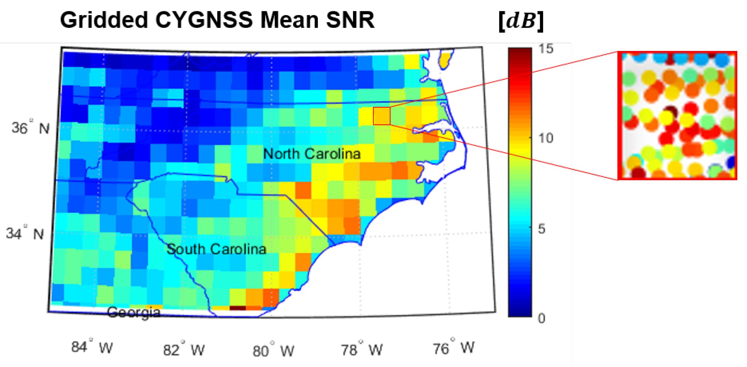
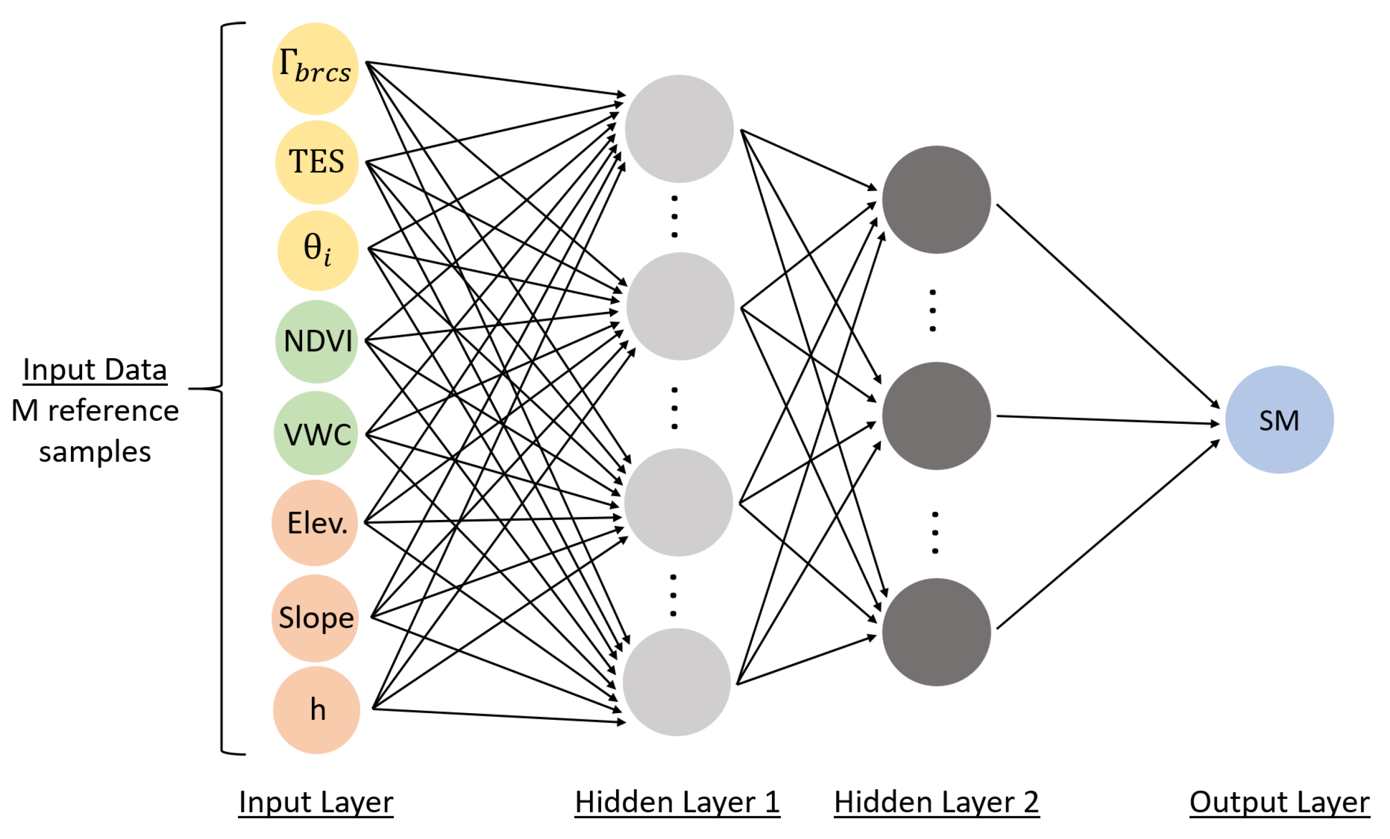
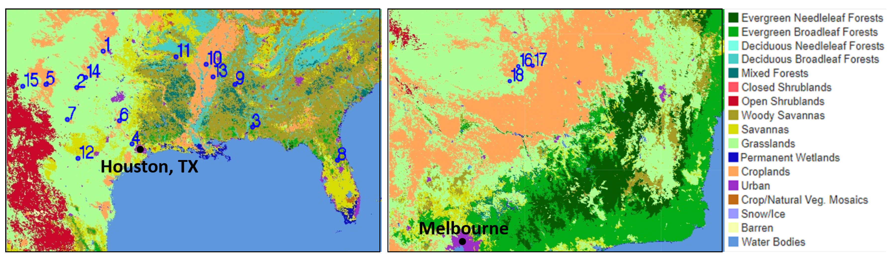
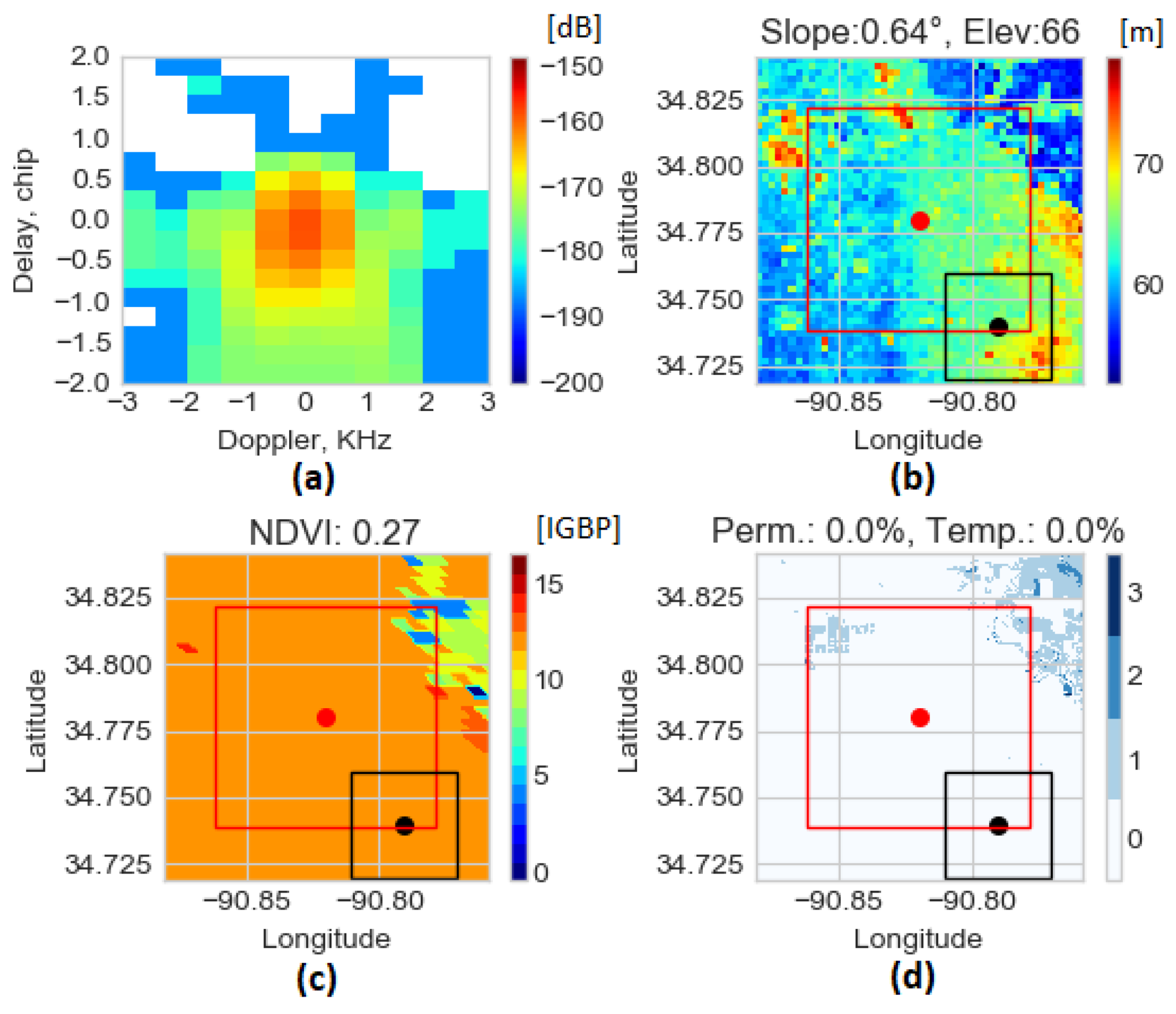
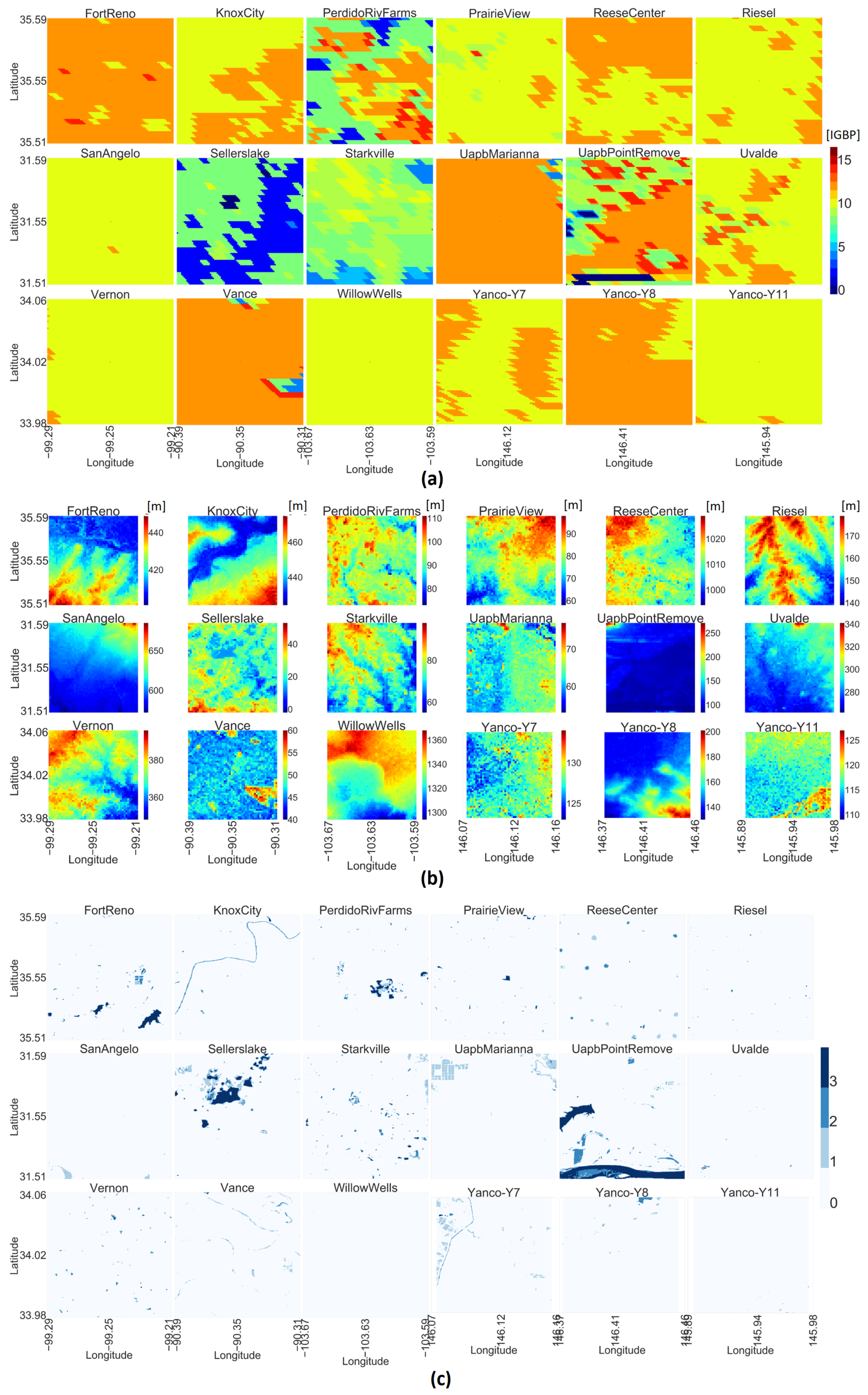
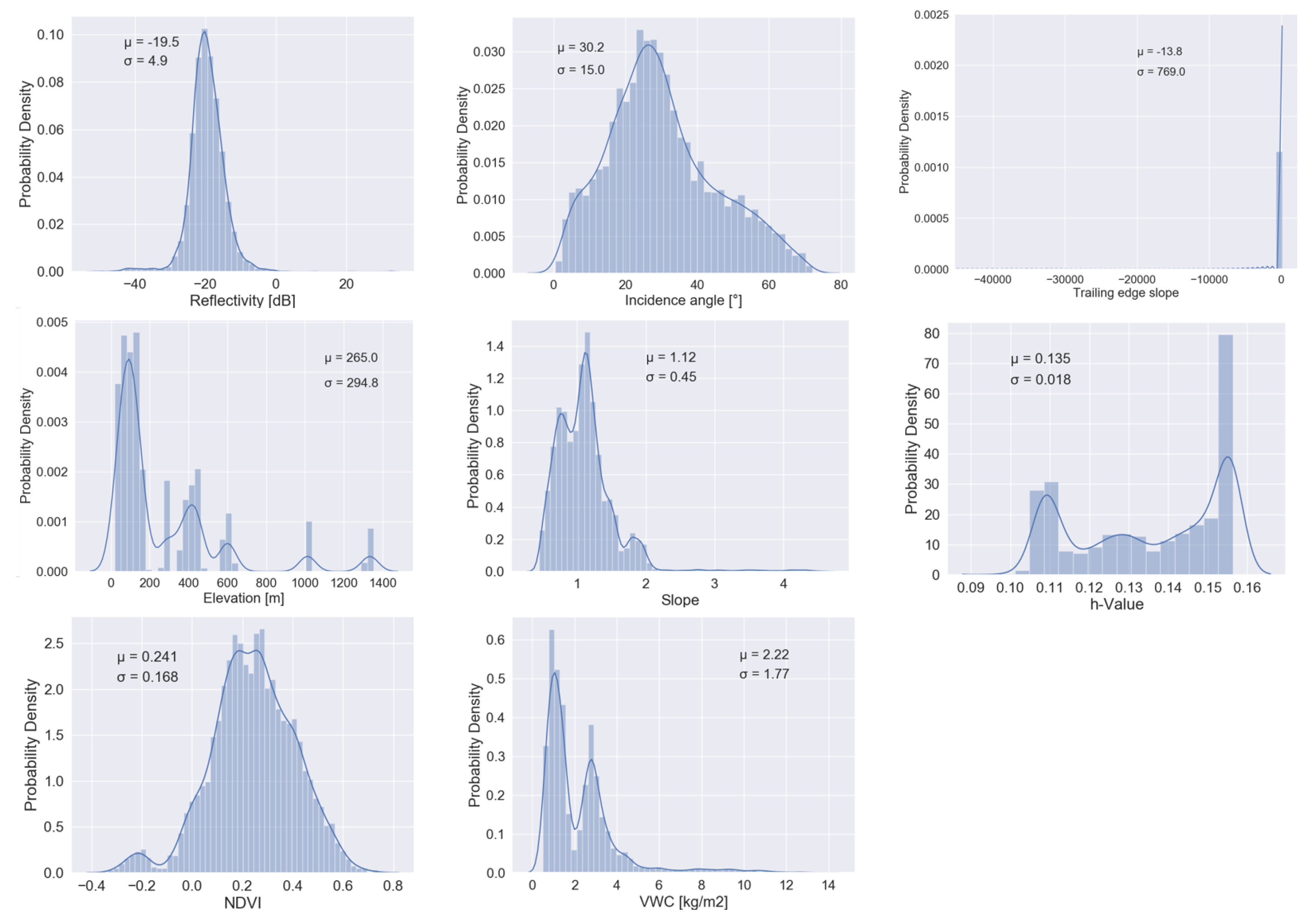
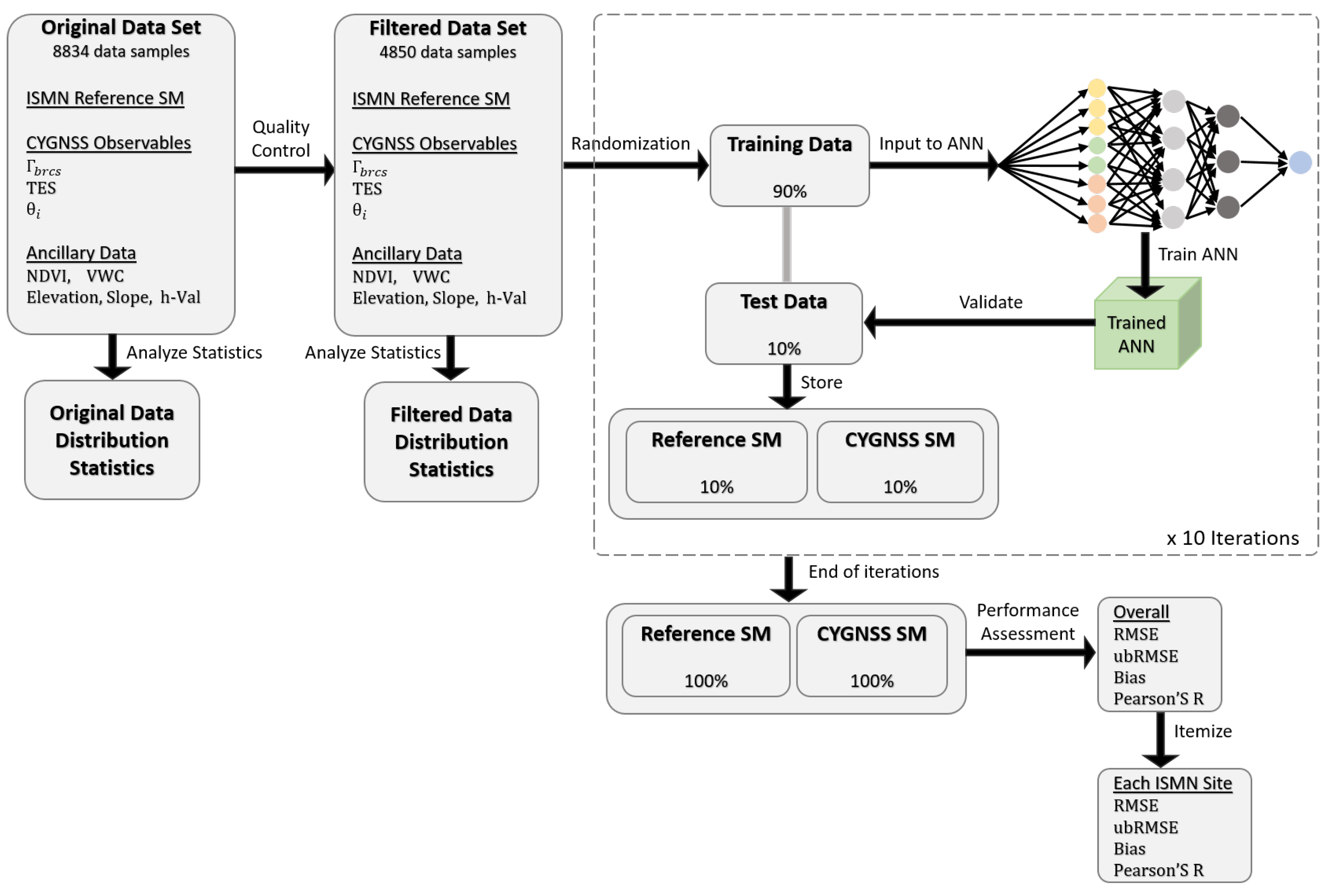
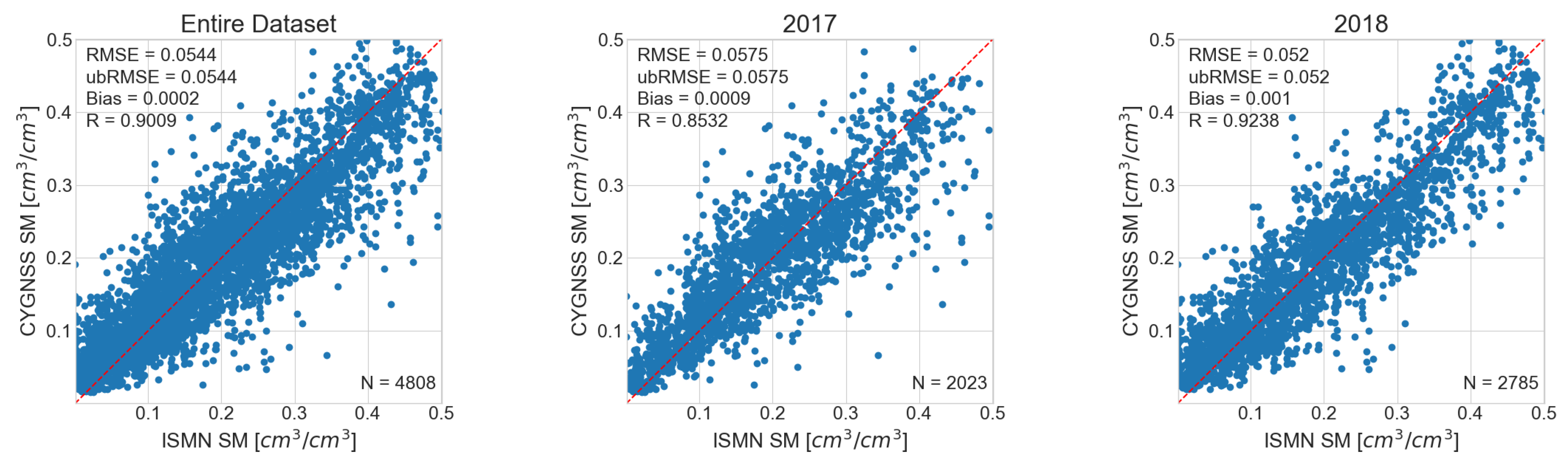
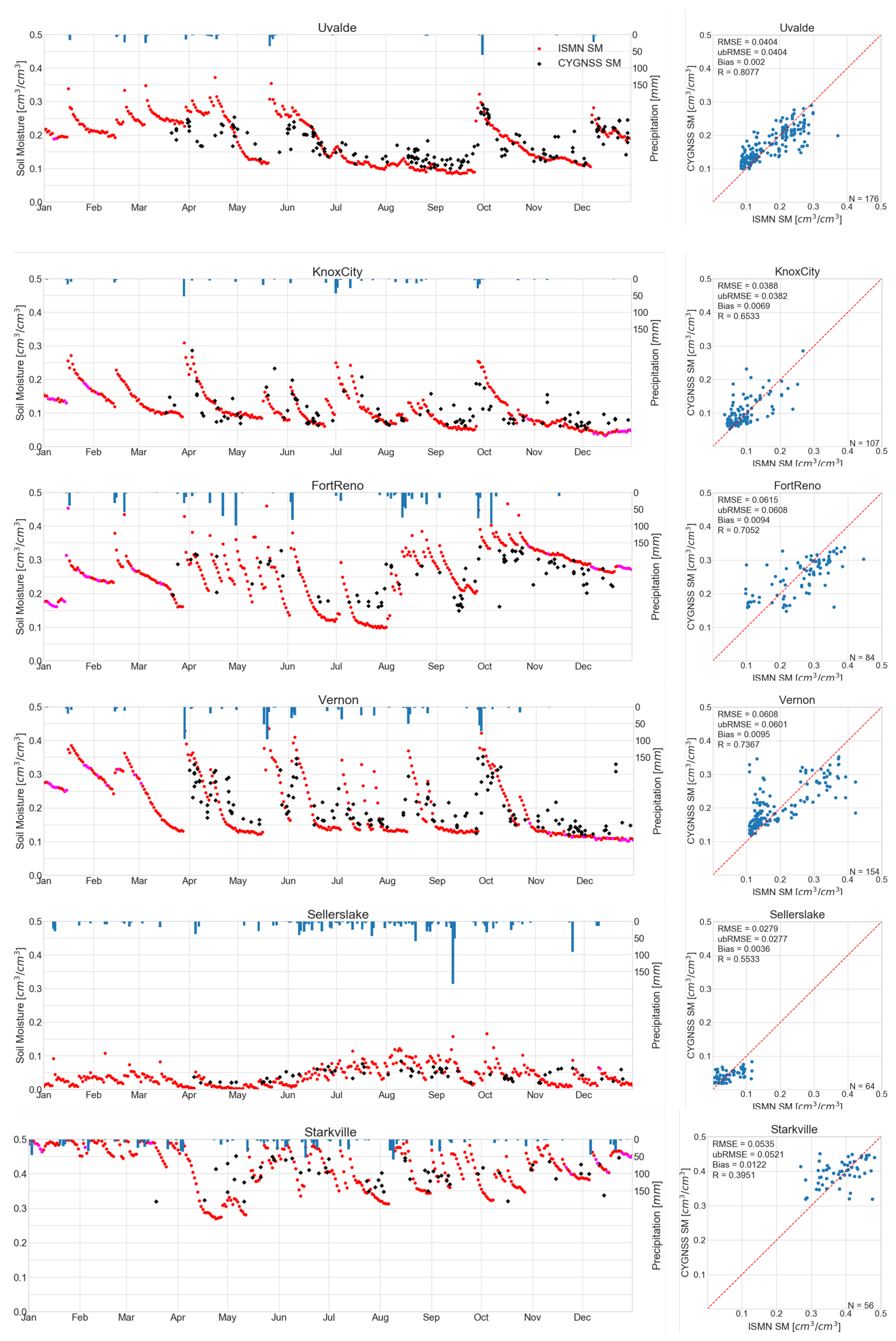
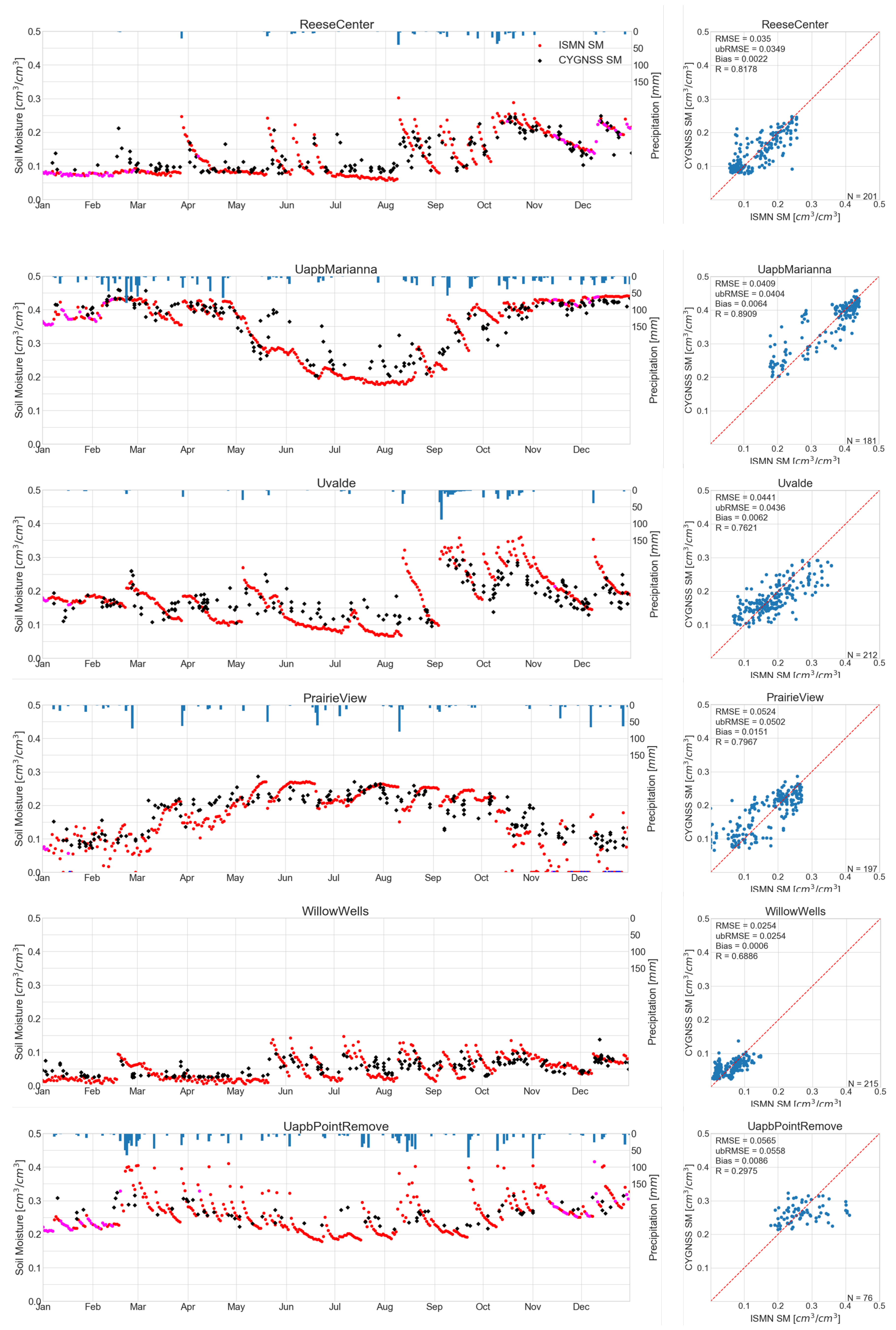
Table A1.
CYGNSS Level 1 data that are used in this study.
| brcs | 17 × 11 array of DDM bin bistatic radar cross section, m. The specular point is located in DDM bin round(brcs_ddm_sp_bin_delay_row), round(brcs_ddm_sp_bin_dopp_col). |
| power_analog | 17 × 11 array of DDM bin analog power, Watts. analog_power is the true power that would have been measured by an ideal (analog) power sensor. power_digital is the power measured by the actual 2-bit sensor, which includes quantization effects. power_analog has been corrected for quantization effects. |
| ddm_snr | DDM signal-to-noise ratio. , where is the maximum value (in raw counts) in a single DDM bin and is the the average per-bin raw noise counts. ddm_snr is in dB. |
| direct_signal_snr | 10log(zenith signal power/zenith signal noise) at ddm_timestamp_utc. |
| sp_lat | SP latitude, in degrees North. |
| sp_lon | SP longitude, in degrees East. |
| rx_to_sp_range | The distance between the CYGNSS spacecraft and the specular point, in meters, at ddm_timestamp_utc. |
| tx_to_sp_range | The distance between the GNSS spacecraft and the specular point, in meters, at ddm_timestamp_utc. |
| sp_inc_angle | SP incidence angle, in degrees. This is the angle between the line normal to the Earth’s surface at the specular point and the line extending from the specular point to the spacecraft. |
| gps_tx_power_db_w | GPS transmit power. Power input to Tx antenna, in dBw. |
| gps_ant_gain_db_i | GPS transmit antenna gain. Antenna gain in the direction of the specular point, in dBi. |
| sp_rx_gain | Specular point Rx antenna gain. The receive antenna gain in the direction of the specular point, in dBi. |
| quality_flags | Per-DDM quality flags. 1 indicates presence of condition. |
References
- Entekhabi, D.; Rodriguez-Iturbe, I.; Castelli, F. Mutual interaction of soil moisture state and atmospheric processes. J. Hydrol. 1996, 184, 3–17. [Google Scholar] [CrossRef]
- Entekhabi, D.; Asrar, G.R.; Betts, A.K.; Beven, K.J.; Bras, R.L.; Duffy, C.J.; Dunne, T.; Koster, R.D.; Lettenmaier, D.P.; McLaughlin, D.B.; et al. An agenda for land surface hydrology research and a call for the second international hydrological decade. Bull. Am. Meteorol. Soc. 1999, 80, 2043–2058. [Google Scholar] [CrossRef]
- Leese, J.; Jackson, T.; Pitman, A.; Dirmeyer, P. GEWEX/BAHC international workshop on soil moisture monitoring, analysis, and prediction for hydrometeorological and hydroclimatological applications. Bull. Am. Meteorol. Soc. 2001, 82, 1423–1430. [Google Scholar] [CrossRef]
- Dobson, M.C.; Ulaby, F.T.; Hallikainen, M.T.; El-Rayes, M.A. Microwave dielectric behavior of wet soil-Part II: Dielectric mixing models. IEEE Trans. Geosci. Remote Sens. 1985, GE-23, 35–46. [Google Scholar] [CrossRef]
- Camps Carmona, A.J. Aplication of Interferometric Radiometry to Earth Observation; Universitat Politècnica de Catalunya: Barcelona, Spain, 1996. [Google Scholar]
- Kerr, Y.H.; Waldteufel, P.; Wigneron, J.P.; Martinuzzi, J.; Font, J.; Berger, M. Soil moisture retrieval from space: The Soil Moisture and Ocean Salinity (SMOS) mission. IEEE Trans. Geosci. Remote Sens. 2001, 39, 1729–1735. [Google Scholar] [CrossRef]
- Entekhabi, D.; Njoku, E.G.; ONeill, P.E.; Kellogg, K.H.; Crow, W.T.; Edelstein, W.N.; Entin, J.K.; Goodman, S.D.; Jackson, T.J.; Johnson, J.; et al. The soil moisture active passive (SMAP) mission. Proc. IEEE 2010, 98, 704–716. [Google Scholar] [CrossRef]
- Kim, S.B.; Van Zyl, J.J.; Johnson, J.T.; Moghaddam, M.; Tsang, L.; Colliander, A.; Dunbar, R.S.; Jackson, T.J.; Jaruwatanadilok, S.; West, R.; et al. Surface soil moisture retrieval using the l-band synthetic aperture radar onboard the soil moisture active–passive satellite and evaluation at core validation sites. IEEE Trans. Geosci. Remote Sens. 2017, 55, 1897–1914. [Google Scholar] [CrossRef]
- Paloscia, S.; Pettinato, S.; Santi, E.; Notarnicola, C.; Pasolli, L.; Reppucci, A. Soil moisture mapping using Sentinel-1 images: Algorithm and preliminary validation. Remote Sens. Environ. 2013, 134, 234–248. [Google Scholar] [CrossRef]
- Aubert, M.; Baghdadi, N.; Zribi, M.; Douaoui, A.; Loumagne, C.; Baup, F.; El Hajj, M.; Garrigues, S. Analysis of TerraSAR-X data sensitivity to bare soil moisture, roughness, composition and soil crust. Remote Sens. Environ. 2011, 115, 1801–1810. [Google Scholar] [CrossRef] [Green Version]
- Zavorotny, V.U.; Gleason, S.; Cardellach, E.; Camps, A. Tutorial on remote sensing using GNSS bistatic radar of opportunity. IEEE Geosci. Remote Sens. Mag. 2014, 2, 8–45. [Google Scholar] [CrossRef]
- Ruf, C.S.; Chew, C.; Lang, T.; Morris, M.G.; Nave, K.; Ridley, A.; Balasubramaniam, R. A new paradigm in earth environmental monitoring with the CYGNSS small satellite constellation. Sci. Rep. 2018, 8, 8782. [Google Scholar] [CrossRef] [PubMed]
- Lowe, S.T.; LaBrecque, J.L.; Zuffada, C.; Romans, L.J.; Young, L.E.; Hajj, G.A. First spaceborne observation of an Earth-reflected GPS signal. Radio Sci. 2002, 37, 1–28. [Google Scholar] [CrossRef]
- Carreno-Luengo, H.; Camps, A.; Via, P.; Munoz, J.F.; Cortiella, A.; Vidal, D.; Jané, J.; Catarino, N.; Hagenfeldt, M.; Palomo, P.; et al. 3Cat-2—An experimental nanosatellite for GNSS-R earth observation: Mission concept and analysis. IEEE J. Sel. Top. Appl. Earth Obs. Remote Sens. 2016, 9, 4540–4551. [Google Scholar] [CrossRef]
- Cardellach, E.; Wickert, J.; Baggen, R.; Benito, J.; Camps, A.; Catarino, N.; Chapron, B.; Dielacher, A.; Fabra, F.; Flato, G.; et al. GNSS transpolar earth reflectometry exploring system (G-TERN): Mission concept. IEEE Access 2018, 6, 13980–14018. [Google Scholar] [CrossRef]
- Castellví, J.; Camps, A.; Corbera, J.; Alamús, R. 3Cat-3/MOTS nanosatellite mission for optical multispectral and GNSS-R earth observation: Concept and analysis. Sensors 2018, 18, 140. [Google Scholar] [CrossRef]
- Unwin, M.; Gleason, S.; Brennan, M. The space GPS reflectometry experiment on the UK disaster monitoring constellation satellite. In Proceedings of the ION-GPS/GNSS, Portland, OR, USA, 9–12 September 2003. [Google Scholar]
- Gleason, S.; Adjrad, M.; Unwin, M. Sensing ocean, ice and land reflected signals from space: Results from the UK-DMC GPS reflectometry experiment. In Proceedings of the 2005 ION GNSS Technical Meeting, Long Beach, CA, USA, 13–16 September 2005. [Google Scholar]
- Camps, A.; Park, H.; Pablos, M.; Foti, G.; Gommenginger, C.P.; Liu, P.W.; Judge, J. Sensitivity of GNSS-R spaceborne observations to soil moisture and vegetation. IEEE J. Sel. Top. Appl. Earth Obs. Remote Sens. 2016, 9, 4730–4742. [Google Scholar] [CrossRef]
- Chew, C.; Shah, R.; Zuffada, C.; Hajj, G.; Masters, D.; Mannucci, A.J. Demonstrating soil moisture remote sensing with observations from the UK TechDemoSat-1 satellite mission. Geophys. Res. Lett. 2016, 43, 3317–3324. [Google Scholar] [CrossRef]
- Ruf, C.S.; Atlas, R.; Chang, P.S.; Clarizia, M.P.; Garrison, J.L.; Gleason, S.; Katzberg, S.J.; Jelenak, Z.; Johnson, J.T.; Majumdar, S.J.; et al. New ocean winds satellite mission to probe hurricanes and tropical convection. Bull. Am. Meteorol. Soc. 2016, 97, 385–395. [Google Scholar] [CrossRef]
- Chew, C.; Small, E. Soil moisture sensing using spaceborne GNSS reflections: Comparison of CYGNSS reflectivity to SMAP soil moisture. Geophys. Res. Lett. 2018, 45, 4049–4057. [Google Scholar] [CrossRef]
- Carreno-Luengo, H.; Luzi, G.; Crosetto, M. Sensitivity of CyGNSS Bistatic Reflectivity and SMAP Microwave Radiometry Brightness Temperature to Geophysical Parameters Over Land Surfaces. IEEE J. Sel. Top. Appl. Earth Obs. Remote Sens. 2019, 12, 107–122. [Google Scholar] [CrossRef]
- Al-Khaldi, M.M.; Johnson, J.T.; O’Brien, A.J.; Balenzano, A.; Mattia, F. Time-Series Retrieval of Soil Moisture Using CYGNSS. IEEE Trans. Geosci. Remote Sens. 2019, 57, 4322–4331. [Google Scholar] [CrossRef]
- Ruf, C.; Chang, P.; Clarizia, M.; Gleason, S.; Jelenak, Z.; Murray, J.; Morris, M.; Musko, S.; Posselt, D.; Provost, D.; et al. Cygnss Handbook; Michigan Publishing: Ann Arbor, MI, USA, 2016; 154p. [Google Scholar]
- Brodzik, M.J.; Billingsley, B.; Haran, T.; Raup, B.; Savoie, M.H. EASE-Grid 2.0: Incremental but significant improvements for Earth-gridded data sets. ISPRS Int. J. Geo-Inf. 2012, 1, 32–45. [Google Scholar] [CrossRef]
- Kim, H.; Lakshmi, V. Use of Cyclone Global Navigation Satellite System (CYGNSS) observations for estimation of soil moisture. Geophys. Res. Lett. 2018, 45, 8272–8282. [Google Scholar] [CrossRef]
- Clarizia, M.P.; Pierdicca, N.; Costantini, F.; Floury, N. Analysis of CYGNSS Data for Soil Moisture Retrieval. IEEE J. Sel. Top. Appl. Earth Obs. Remote Sens. 2019, 12, 2227–2235. [Google Scholar] [CrossRef]
- De Roo, R.D.; Ulaby, F.T. Bistatic specular scattering from rough dielectric surfaces. IEEE Trans. Antennas Propag. 1994, 42, 220–231. [Google Scholar] [CrossRef]
- Voronovich, A.G.; Zavorotny, V.U. Bistatic radar equation for signals of opportunity revisited. IEEE Trans. Geosci. Remote Sens. 2017, 56, 1959–1968. [Google Scholar] [CrossRef]
- Kurum, M.; Deshpande, M.; Joseph, A.T.; O’Neill, P.E.; Lang, R.H.; Eroglu, O. SCoBi-Veg: A generalized bistatic scattering model of reflectometry from vegetation for Signals of Opportunity applications. IEEE Trans. Geosci. Remote Sens. 2018, 57, 1049–1068. [Google Scholar] [CrossRef]
- Zavorotny, V.U.; Voronovich, A.G. Scattering of GPS signals from the ocean with wind remote sensing application. IEEE Trans. Geosci. Remote Sens. 2000, 38, 951–964. [Google Scholar] [CrossRef] [Green Version]
- Ruf, C.; Redfern, J.; Butler, T.; McKague, D.; Gleason, S. Level 1B DDM Calibration Algorithm Theoretical Basis Document Rev. 2. 2018. Available online: http://clasp-research.engin.umich.edu/missions/cygnss/reference/148-0137_ATBD_L1B_DDMCalibration_Rev2_Aug2018_release.pdf (accessed on 24 July 2019).
- Eroglu, O.; Kurum, M.; Ball, J. Response of GNSS-R on Dynamic Vegetated Terrain Conditions. IEEE J. Sel. Top. Appl. Earth Obs. Remote Sens. 2019, 12, 1599–1611. [Google Scholar] [CrossRef]
- Rodriguez-Alvarez, N.; Podest, E.; Jensen, K.; McDonald, K.C. Classifying Inundation in a Tropical Wetlands Complex with GNSS-R. Remote Sens. 2019, 11, 1053. [Google Scholar] [CrossRef]
- Jackson, T.; Schmugge, T. Vegetation effects on the microwave emission of soils. Remote Sens. Environ. 1991, 36, 203–212. [Google Scholar] [CrossRef]
- Choudhury, B.; Schmugge, T.J.; Chang, A.; Newton, R. Effect of surface roughness on the microwave emission from soils. J. Geophys. Res. Oceans 1979, 84, 5699–5706. [Google Scholar] [CrossRef]
- O’Neill, P.; Chan, S.; Njoku, E.; Jackson, T.; Bindlish, R. Soil Moisture Active Passive (SMAP) Algorithm Theoretical Basis Document Level 2 & 3 Soil Moisture (Passive) Data Products; Jet Propulsion Laboratory, California Institute of Technology: Pasadena, CA, USA, 2014. [Google Scholar]
- Chan, S.; Bindlish, R.; Hunt, R.; Jackson, T.; Kimball, J. Vegetation Water Content; Jet Propulsion Laboratory, California Institute of Technology: Pasadena, CA, USA, 2013. [Google Scholar]
- Mironov, V.L.; De Roo, R.D.; Savin, I.V. Temperature-dependable microwave dielectric model for an Arctic soil. IEEE Trans. Geosci. Remote Sens. 2010, 48, 2544–2556. [Google Scholar] [CrossRef]
- Wang, J.R.; Schmugge, T.J. An empirical model for the complex dielectric permittivity of soils as a function of water content. IEEE Trans. Geosci. Remote Sens. 1980, GE-18, 288–295. [Google Scholar] [CrossRef]
- Gleason, S.; Ruf, C.S.; O’Brien, A.J.; McKague, D.S. The CYGNSS Level 1 calibration algorithm and error analysis based on on-orbit measurements. IEEE J. Sel. Top. Appl. Earth Obs. Remote Sens. 2018, 12, 37–49. [Google Scholar] [CrossRef]
- Twomey, S. Introduction to the Mathematics of Inversion in Remote Sensing and Indirect Measurements; Elsevier: Amsterdam, The Netherlands, 2013; Volume 3. [Google Scholar]
- Egido, A.; Caparrini, M.; Ruffini, G.; Paloscia, S.; Santi, E.; Guerriero, L.; Pierdicca, N.; Floury, N. Global navigation satellite systems reflectometry as a remote sensing tool for agriculture. Remote Sens. 2012, 4, 2356–2372. [Google Scholar] [CrossRef]
- Kerr, Y.; Waldteufel, P.; Richaume, P.; Davenport, I.; Ferrazzoli, P.; Wigneron, J. SMOS Level 2 Processor Soil Moisture Algorithm Theoretical Basis Document (ATBD); SO-TN-ESL-SM-GS-0001, V5. a, 15/03; SM-ESL (CBSA), CESBIO: Toulouse, France, 2006. [Google Scholar]
- Xie, Y.; Sha, Z.; Yu, M.; Bai, Y.; Zhang, L. A comparison of two models with Landsat data for estimating above ground grassland biomass in Inner Mongolia, China. Ecol. Model. 2009, 220, 1810–1818. [Google Scholar] [CrossRef]
- Ali, I.; Greifeneder, F.; Stamenkovic, J.; Neumann, M.; Notarnicola, C. Review of machine learning approaches for biomass and soil moisture retrievals from remote sensing data. Remote Sens. 2015, 7, 16398–16421. [Google Scholar] [CrossRef]
- Hornik, K.; Stinchcombe, M.; White, H. Multilayer feedforward networks are universal approximators. Neural Netw. 1989, 2, 359–366. [Google Scholar] [CrossRef]
- Vermote, E.; Wolfe, R. MOD09GA MODIS/Terra Surface Reflectance Daily L2G Global 1 km and 500 m SIN Grid V006. NASA EOSDIS Land Processes DAAC. 2015. Available online: https://lpdaac. usgs. gov/dataset_ discovery/modis/modis_products_table/mod09ga_v006 (accessed on 16 October 2016).
- Jarvis, A.; Reuter, H.I.; Nelson, A.; Guevara, E. Hole-Filled SRTM for the Globe Version 4, Available from the CGIAR-CSI SRTM 90m Database; CGIAR Consortium for Spatial Information: Montpellier, France, 2008. [Google Scholar]
- Hinton, G.E. Connectionist learning procedures. In Machine Learning; Elsevier: Amsterdam, The Netherlands, 1990; pp. 555–610. [Google Scholar]
- Glorot, X.; Bengio, Y. Understanding the difficulty of training deep feedforward neural networks. In Proceedings of the Thirteenth International Conference on Artificial Intelligence and Statistics, Sardinia, Italy, 13–15 May 2010; pp. 249–256. [Google Scholar]
- Nair, V.; Hinton, G.E. Rectified linear units improve restricted boltzmann machines. In Proceedings of the 27th International Conference on Machine Learning (ICML-10), Haifa, Israel, 21–24 June 2010; pp. 807–814. [Google Scholar]
- Karlik, B.; Olgac, A.V. Performance analysis of various activation functions in generalized MLP architectures of neural networks. Int. J. Artif. Intell. Expert Syst. 2011, 1, 111–122. [Google Scholar]
- Kingma, D.P.; Ba, J. Adam: A method for stochastic optimization. arXiv 2014, arXiv:1412.6980. [Google Scholar]
- Dorigo, W.; Gruber, A.; De Jeu, R.; Wagner, W.; Stacke, T.; Loew, A.; Albergel, C.; Brocca, L.; Chung, D.; Parinussa, R.; et al. Evaluation of the ESA CCI soil moisture product using ground-based observations. Remote Sens. Environ. 2015, 162, 380–395. [Google Scholar] [CrossRef]
- Schaefer, G.L.; Cosh, M.H.; Jackson, T.J. The USDA natural resources conservation service soil climate analysis network (SCAN). J. Atmos. Ocean. Technol. 2007, 24, 2073–2077. [Google Scholar] [CrossRef]
- Smith, A.; Walker, J.P.; Western, A.W.; Young, R.; Ellett, K.; Pipunic, R.; Grayson, R.; Siriwardena, L.; Chiew, F.; Richter, H. The Murrumbidgee soil moisture monitoring network data set. Water Resour. Res. 2012, 48. [Google Scholar] [CrossRef]
- Friedl, M.; Sulla-Menashe, D. MCD12Q1 MODIS/Terra+ Aqua Land Cover Type Yearly L3 Global 500m SIN Grid V006 [Data Set]; NASA EOSDIS Land Processes DAAC: Sioux Falls, SD, USA, 2015. [Google Scholar]
- Gorelick, N.; Hancher, M.; Dixon, M.; Ilyushchenko, S.; Thau, D.; Moore, R. Google Earth Engine: Planetary-scale geospatial analysis for everyone. Remote Sens. Environ. 2017, 202, 18–27. [Google Scholar] [CrossRef]
- Pekel, J.F.; Cottam, A.; Gorelick, N.; Belward, A.S. High-resolution mapping of global surface water and its long-term changes. Nature 2016, 540, 418. [Google Scholar] [CrossRef]
- Vermote, E.; Justice, C.; Csiszar, I.; Eidenshink, J.; Myneni, R.; Baret, F.; Masuoka, E.; Wolfe, R.; Claverie, M. NOAA Climate Data Record (CDR) of Normalized Difference Vegetation Index (NDVI), Version 4; NOAA National Climatic Data Center: Asheville, NC, USA, 2014. [Google Scholar]
- Pukelsheim, F. The three sigma rule. Am. Stat. 1994, 48, 88–91. [Google Scholar]
- Wen, J.; Liu, Q.; Xiao, Q.; Liu, Q.; You, D.; Hao, D.; Wu, S.; Lin, X. Characterizing land surface anisotropic reflectance over rugged terrain: A review of concepts and recent developments. Remote Sens. 2018, 10, 370. [Google Scholar] [CrossRef]
- Picard, R.R.; Cook, R.D. Cross-validation of regression models. J. Am. Stat. Assoc. 1984, 79, 575–583. [Google Scholar] [CrossRef]
- Entekhabi, D.; Reichle, R.H.; Koster, R.D.; Crow, W.T. Performance metrics for soil moisture retrievals and application requirements. J. Hydrometeorol. 2010, 11, 832–840. [Google Scholar] [CrossRef]
Figure 1.
Multiple CYGNSS observations (uncalibrated DDM SNR) that are averaged into the SMAP grids. Data are from 14–18 September 2018 over North Carolina, USA (The landfall of the Hurricane Florence was on 14 September 2018).
Figure 1.
Multiple CYGNSS observations (uncalibrated DDM SNR) that are averaged into the SMAP grids. Data are from 14–18 September 2018 over North Carolina, USA (The landfall of the Hurricane Florence was on 14 September 2018).

Figure 2.
Artificial Neural Network with two hidden layers. Input features and the output node are color-coded with respect to separate data sets from which the parameter values were derived. ( is the reflectivity calculated from BRCS and will be defined later.)
Figure 2.
Artificial Neural Network with two hidden layers. Input features and the output node are color-coded with respect to separate data sets from which the parameter values were derived. ( is the reflectivity calculated from BRCS and will be defined later.)

Figure 3.
ISMN site locations with the IGBP land cover classification in the background. (Left): SCAN sites from USA, (Middle): OzNet sites from Australia, (Right): IGBP land cover classification color-code. Indices are same with Table 2.
Figure 3.
ISMN site locations with the IGBP land cover classification in the background. (Left): SCAN sites from USA, (Middle): OzNet sites from Australia, (Right): IGBP land cover classification color-code. Indices are same with Table 2.

Figure 4.
Example grid analysis from a CYGNSS observation over the SCAN site Uapb-Marianna on day-of year (DOY) 71, 2018. The red square is the 9-km grid cell that centers the ISMN site (red dot). The black square is the 4-km grid cells that center the CYGNSS observation SP (black dot) that could fall into anywhere in the 9-km grid. (a) DDM ; (b) digital elevation model [m]. Mean slope and elevation values calculated from 4-km grid are also shown; (c) IGBP land covers [IGBP]. The color scale for the IGBP land cover is the same as Figure 3. Mean NDVI calculated from the 4-km grid is also shown; (d) inland water bodies [Pekel indices [61]. Permanent and temporary water body percentages within the 4-km grid are also shown.

Figure 5.
Ancillary data visualization for 18 ISMN sites. (a) IGBP land cover [IGBP]. The land cover color scale is the same as in Figure 3; (b) DEM [m]. DEM color scale is generated separately per each ISMN site; (c) inland water bodies [Pekel indices [61]. The inland water body color scale is the same as in Figure 4.

Figure 6.
Distributions of the input features (before quality control flags applied). Application of quality controls did not result in large variations. Distribution statistics are also given in each plot.
Figure 6.
Distributions of the input features (before quality control flags applied). Application of quality controls did not result in large variations. Distribution statistics are also given in each plot.

Figure 7.
Flowchart showing the training and validation of the CYGNSS SM retrieval algorithm.

Figure 8.
Scatter plots of SM retrievals for the entire data set, year 2017, and year 2018. RMSE, ubRMSE, and bias are given in [cm/cm]. Pearson’s R is also provided. N is the number of data points.
Figure 8.
Scatter plots of SM retrievals for the entire data set, year 2017, and year 2018. RMSE, ubRMSE, and bias are given in [cm/cm]. Pearson’s R is also provided. N is the number of data points.

Figure 9.
SM retrievals for 2017. In situ SM data are color-coded such that magenta and blue circles correspond to days with freeze temperatures and invalid data, respectively. Scatter plots are also given.
Figure 9.
SM retrievals for 2017. In situ SM data are color-coded such that magenta and blue circles correspond to days with freeze temperatures and invalid data, respectively. Scatter plots are also given.

Figure 10.
SM retrievals for year 2018. In situ SM data are color-coded such that magenta and blue circles correspond to days with freeze temperatures and invalid data, respectively. Scatter plots are also given.
Figure 10.
SM retrievals for year 2018. In situ SM data are color-coded such that magenta and blue circles correspond to days with freeze temperatures and invalid data, respectively. Scatter plots are also given.

| Parameter | Value |
|---|---|
| Orbit | Non-synchronous |
| Altitude | ∼520 km |
| Period | 95 min |
| Spatial Resolution | ∼25 km × 25 km (incoherent), ∼0.6 km × 6.6 km (coherent, theoretical minimum) |
| Revisit Times | 3 h median, 7 h mean (over the ocean) |
| Frequency | 1.57542 GHz |
| Polarization | Left-hand circularly polarized (LHCP) (Down-looking GNSS-R antenna) |
Table 2.
Soil moisture sites that are analyzed in this study. Elevation (in meters) and slope values are calculated as mean values over the 9-km grid.
Table 2.
Soil moisture sites that are analyzed in this study. Elevation (in meters) and slope values are calculated as mean values over the 9-km grid.
| ISMN Site | Location | Lat, Lon | Land Cover (IGBP) | Elev. | Slope |
|---|---|---|---|---|---|
| 1 - Fort Reno (SCAN) | Oklahoma, US | 35.55, −98.02 | Croplands | 420 | 1.15 |
| 2 - Knox City (SCAN) | Texas, US | 33.45, −99.87 | Croplands, Grasslands | 446 | 0.98 |
| 3 - Perdido Riv Farms (SCAN) | Alabama, US | 31.11, −87.55 | Crop., Savan., Forests | 94 | 1.21 |
| 4 - Prairie View (SCAN) | Texas, US | 30.08, −95.98 | Grass., Savan., Crop. | 80 | 1.12 |
| 5 - Reese Center (SCAN) | Texas, US | 33.62, −102.04 | Croplands, Grasslands | 1014 | 1.14 |
| 6 - Riesel (SCAN) | Texas, US | 31.48, −96.88 | Grasslands, Croplands | 161 | 1.22 |
| 7 - San Angelo (SCAN) | Texas, US | 31.55, −100.51 | Grasslands | 600 | 0.81 |
| 8 - Sellers Lake (SCAN) | Florida, US | 29.10, −81.63 | Forests, Savannas | 24 | 1.87 |
| 9 - Starkville (SCAN) | Mississippi, US | 33.63, −88.77 | Savan., Forests, Grass. | 75 | 1.46 |
| 10 - Uapb Marianna (SCAN) | Arkansas, US | 34.78, −90.82 | Croplands | 63 | 0.84 |
| 11 - Uapb Point Remove (SCAN) | Arkansas, US | 35.21, −92.92 | Croplands, Grasslands | 99 | 1.28 |
| 12 - Uvalde (SCAN) | Texas, US | 29.22, −99.76 | Grasslands, Croplands | 285 | 1.21 |
| 13 - Vance (SCAN) | Mississippi, US | 34.07, −90.35 | Croplands, Forests | 47 | 0.81 |
| 14 - Vernon (SCAN) | Texas, US | 34.02, −99.25 | Grasslands, Croplands | 373 | 1.28 |
| 15 - Willow Wells (SCAN) | New Mexico, US | 33.53 −103.63 | Grasslands | 1336 | 0.97 |
| 16 - Yanco-Y7 (OzNet) | Yanco, Australia | −34.85, 146.12 | Grasslands, Croplands | 128 | 0.55 |
| 17 - Yanco-Y8 (OzNet) | Yanco, Australia | −34.85, 146.41 | Croplands, Grasslands | 150 | 0.94 |
| 18 - Yanco-Y11 (OzNet) | Yanco, Australia | −35.11, 145.94 | Grasslands, Croplands | 114 | 0.75 |
Table 3.
The separate, ideal impact of each quality control is shown as percent changes to the original data set: If each quality flag was applied alone to the original data set, the percent changes to the original data set would be as given from the sixth to tenth columns (CYG.: CYGNSS quality flags, : < 65, : Positive receiver gain, Peak: DDM peak delay bin rows in [7, 10], Water: Removal of inland water bodies). For reference, the initial numbers of data samples before the application of the quality controls are given annually in the second and third columns. Percent losses in the data set due to the actual application of the entire quality controls are also given in the fourth and fifth columns. Overall data set sizes and percent changes are given in the bottom-most row. Year 2017 data for the ISMN sites, Reese Center and Willow Wells, have not been analyzed because these stations are located over 1000 meters, and CYGNSS has an elevation upper limit of 600 m for the SP calculation algorithm until December 2017 [22]. Year 2018 data for the Riesel station have not been analyzed as well due to large blocks of invalid SM data.
| ISMN Site | Initial # | Final (%) | CYG. | Peak | Water | ||||
|---|---|---|---|---|---|---|---|---|---|
| 2017 | 2018 | 2017 | 2018 | (%) | (%) | (%) | (%) | (%) | |
| Fort Reno | 271 | 275 | 69.0 | 66.9 | 5.2 | 2.3 | 30.4 | 11.4 | 53.1 |
| Knox City | 257 | 281 | 58.4 | 56.2 | 6.9 | 2.6 | 27.9 | 9.6 | 37.2 |
| Perdido Riv F. | 248 | 306 | 55.6 | 52.9 | 6.4 | 2.2 | 24.6 | 11.7 | 38.9 |
| Prairie View | 292 | 289 | 31.2 | 31.8 | 7.3 | 0.9 | 24.9 | 9.6 | 4.9 |
| Reese Center | — | 283 | — | 29.0 | 6.4 | 1.4 | 21.9 | 6.7 | 4.24 |
| Riesel | 252 | — | 33.3 | — | 6.8 | 0.4 | 27.8 | 12.7 | 0.0 |
| San Angelo | 249 | 308 | 48.6 | 29.3 | 6.3 | 0.2 | 21.7 | 20.9 | 5.7 |
| Sellers Lake | 246 | 255 | 74.0 | 69.8 | 7.0 | 2.3 | 19.6 | 12.0 | 61.9 |
| Starkville | 207 | 272 | 72.9 | 74.3 | 6.7 | 1.7 | 26.6 | 12.9 | 61.4 |
| Uapb-Marianna | 226 | 267 | 37.2 | 32.2 | 9.1 | 1.1 | 26.8 | 13.1 | 7.9 |
| Uapb–Point R. | 270 | 306 | 73.0 | 75.2 | 5.1 | 1.6 | 28.7 | 9.6 | 64.2 |
| Uvalde | 236 | 298 | 25.4 | 28.9 | 5.7 | 1.4 | 23.7 | 10.0 | 0.0 |
| Vance | 226 | 330 | 41.6 | 40.3 | 7.1 | 2.8 | 29.4 | 19.0 | 13.4 |
| Vernon | 232 | 294 | 33.6 | 28.6 | 5.9 | 1.5 | 26.6 | 9.8 | 1.2 |
| Willow Wells | — | 292 | — | 26.4 | 5.1 | 0.3 | 22.6 | 7.9 | 1.37 |
| Yanco-Y7 | 210 | 287 | 34.8 | 41.8 | 6.2 | 0.9 | 26.7 | 7.7 | 13.5 |
| Yanco-Y8 | 215 | 322 | 40.4 | 37.0 | 7.2 | 2.0 | 26.8 | 8.7 | 13.3 |
| Yanco-Y11 | 235 | 297 | 30.6 | 31.7 | 5.9 | 2.7 | 27.6 | 8.7 | 0.0 |
| Overall | 3872 | 4962 | 47.8 | 43.9 | 6.5 | 1.6 | 25.9 | 11.2 | 22.9 |
Table 4.
Assessment of the input feature contributions to the learning process. The statistical performance metrics are given for the entire data set. (*) The bottom-most row shows the optimal performance, which in turn has the input features set that is used in this study.
Table 4.
Assessment of the input feature contributions to the learning process. The statistical performance metrics are given for the entire data set. (*) The bottom-most row shows the optimal performance, which in turn has the input features set that is used in this study.
| Input Features | RMSE | ubRMSE | Bias | R |
|---|---|---|---|---|
| (i) + TES + + NDVI + VWC + Elev. + Slope + h | 0.0579 | 0.0579 | 0.0006 | 0.8869 |
| (ii) + TES + + NDVI + VWC + Elev. + Slope + h | 0.0635 | 0.0635 | 0.0006 | 0.8619 |
| (iii) + TES + + NDVI + VWC + Elev. + Slope + h | 0.0603 | 0.0603 | 0.0007 | 0.8763 |
| (iv) + + TES + + NDVI + VWC + Elev. + Slope + h | 0.0547 | 0.0547 | 0.0010 | 0.9001 |
| (v) + TES + NDVI + VWC + Elev. + Slope + h | 0.0549 | 0.0549 | 0.0013 | 0.9001 |
| (vi) + + NDVI + VWC + Elev. + Slope + h | 0.0596 | 0.0596 | 0.0012 | 0.8920 |
| (vii) + TES + + VWC + Elev. + Slope + h | 0.0554 | 0.0554 | 0.0001 | 0.8970 |
| (viii) + TES + + NDVI + Elev. + Slope + h | 0.0595 | 0.0595 | 0.0001 | 0.8794 |
| (ix) + TES + + NDVI + VWC + Slope + h | 0.0579 | 0.0579 | 0.0003 | 0.8869 |
| (x) + TES + + NDVI + VWC + Elev. + h | 0.0564 | 0.0564 | 0.0003 | 0.8972 |
| (xi) + TES + + NDVI + VWC + Elev. + Slope | 0.0548 | 0.0548 | 0.0001 | 0.8995 |
| (*) + TES + + NDVI + VWC + Elev. + Slope + h | 0.0544 | 0.0544 | 0.0002 | 0.9009 |
Table 5.
SM retrieval algorithm performance statistics. RMSE, ubRMSE, and bias are expressed in [cm/cm]. Pearson’s R is also provided.
Table 5.
SM retrieval algorithm performance statistics. RMSE, ubRMSE, and bias are expressed in [cm/cm]. Pearson’s R is also provided.
| 2017 | 2018 | |||||||
|---|---|---|---|---|---|---|---|---|
| ISMN Site | RMSE | ubRMSE | Bias | R | RMSE | ubRMSE | Bias | R |
| Fort Reno | 0.0615 | 0.0608 | 0.0094 | 0.7052 | 0.0521 | 0.0520 | 0.0013 | 0.8019 |
| Knox City | 0.0388 | 0.0382 | 0.0069 | 0.6533 | 0.0503 | 0.0492 | 0.0108 | 0.7640 |
| Perdido Riv Farms | 0.0493 | 0.0487 | 0.0080 | 0.5986 | 0.0521 | 0.0513 | 0.0091 | 0.4417 |
| Prairie View | 0.0465 | 0.0455 | 0.0099 | 0.5897 | 0.0524 | 0.0502 | 0.0151 | 0.7967 |
| Reese Center | - | - | - | - | 0.0350 | 0.0349 | 0.0022 | 0.8178 |
| Riesel | 0.0947 | 0.0918 | 0.0236 | 0.6706 | - | - | - | - |
| San Angelo | 0.0615 | 0.0606 | 0.0103 | 0.3825 | 0.0705 | 0.0687 | 0.0158 | 0.6290 |
| Sellers Lake | 0.0279 | 0.0277 | 0.0036 | 0.5533 | 0.0252 | 0.0246 | 0.0059 | 0.4171 |
| Starkville | 0.0535 | 0.0521 | 0.0122 | 0.3951 | 0.0621 | 0.0614 | 0.0415 | 0.3609 |
| Uapb-Marianna | 0.0522 | 0.0514 | 0.0088 | 0.5994 | 0.0409 | 0.0404 | 0.0064 | 0.8909 |
| Uapb–Point Remove | 0.0442 | 0.0363 | 0.0253 | 0.3350 | 0.0565 | 0.0558 | 0.0086 | 0.2975 |
| Uvalde | 0.0404 | 0.0404 | 0.0019 | 0.8077 | 0.0441 | 0.0436 | 0.0062 | 0.7621 |
| Vance | 0.0789 | 0.0776 | 0.0142 | 0.5764 | 0.0750 | 0.0744 | 0.0095 | 0.8489 |
| Willow Wells | - | - | - | - | 0.0254 | 0.0254 | 0.0006 | 0.6886 |
| Vernon | 0.0608 | 0.0601 | 0.0095 | 0.7367 | 0.0567 | 0.0565 | 0.0056 | 0.8506 |
| Yanco-Y7 | 0.0417 | 0.0411 | 0.0074 | 0.5645 | 0.0358 | 0.0354 | 0.0057 | 0.7348 |
| Yanco-Y8 | 0.0453 | 0.0444 | 0.0089 | 0.4662 | 0.0565 | 0.0553 | 0.0113 | 0.2529 |
| Yanco-Y11 | 0.0604 | 0.0602 | 0.0041 | 0.4410 | 0.0571 | 0.0571 | 0.0008 | 0.6170 |
| Overall | 0.0575 | 0.0575 | 0.0009 | 0.8532 | 0.0520 | 0.0520 | 0.0010 | 0.9238 |
© 2019 by the authors. Licensee MDPI, Basel, Switzerland. This article is an open access article distributed under the terms and conditions of the Creative Commons Attribution (CC BY) license (http://creativecommons.org/licenses/by/4.0/).
Share and Cite
MDPI and ACS Style
Eroglu, O.; Kurum, M.; Boyd, D.; Gurbuz, A.C. High Spatio-Temporal Resolution CYGNSS Soil Moisture Estimates Using Artificial Neural Networks. Remote Sens. 2019, 11, 2272. https://0-doi-org.brum.beds.ac.uk/10.3390/rs11192272
AMA Style
Eroglu O, Kurum M, Boyd D, Gurbuz AC. High Spatio-Temporal Resolution CYGNSS Soil Moisture Estimates Using Artificial Neural Networks. Remote Sensing. 2019; 11(19):2272. https://0-doi-org.brum.beds.ac.uk/10.3390/rs11192272
Chicago/Turabian StyleEroglu, Orhan, Mehmet Kurum, Dylan Boyd, and Ali Cafer Gurbuz. 2019. "High Spatio-Temporal Resolution CYGNSS Soil Moisture Estimates Using Artificial Neural Networks" Remote Sensing 11, no. 19: 2272. https://0-doi-org.brum.beds.ac.uk/10.3390/rs11192272
Note that from the first issue of 2016, this journal uses article numbers instead of page numbers. See further details here.