Evaluation of Approaches for Mapping Tidal Wetlands of the Chesapeake and Delaware Bays


1
Department of Earth and Atmospheric Sciences, The City College of New York, City University of New York, New York, NY 10031, USA
2
Earth and Environmental Sciences Program, The Graduate Center, City University of New York, New York, NY 10016, USA
3
NASA Goddard Space Flight Center, Greenbelt, MD 20771, USA
4
Carbon Cycle and Ecosystems Group, Jet Propulsion Laboratory, California Institute of Technology, Pasadena, CA 91109, USA
*
Author to whom correspondence should be addressed.
Remote Sens. 2019, 11(20), 2366; https://0-doi-org.brum.beds.ac.uk/10.3390/rs11202366
Submission received: 1 July 2019
/
Revised: 27 September 2019
/
Accepted: 3 October 2019
/
Published: 12 October 2019
(This article belongs to the Special Issue Satellite-Based Wetland Observation)
Abstract
:The spatial extent and vegetation characteristics of tidal wetlands and their change are among the biggest unknowns and largest sources of uncertainty in modeling ecosystem processes and services at the land-ocean interface. Using a combination of moderate-high spatial resolution (≤30 meters) optical and synthetic aperture radar (SAR) satellite imagery, we evaluated several approaches for mapping and characterization of wetlands of the Chesapeake and Delaware Bays. Sentinel-1A, Phased Array type L-band Synthetic Aperture Radar (PALSAR), PALSAR-2, Sentinel-2A, and Landsat 8 imagery were used to map wetlands, with an emphasis on mapping tidal marshes, inundation extents, and functional vegetation classes (persistent vs. non-persistent). We performed initial characterizations at three target wetlands study sites with distinct geomorphologies, hydrologic characteristics, and vegetation communities. We used findings from these target wetlands study sites to inform the selection of timeseries satellite imagery for a regional scale random forest-based classification of wetlands in the Chesapeake and Delaware Bays. Acquisition of satellite imagery, raster manipulations, and timeseries analyses were performed using Google Earth Engine. Random forest classifications were performed using the R programming language. In our regional scale classification, estuarine emergent wetlands were mapped with a producer’s accuracy greater than 88% and a user’s accuracy greater than 83%. Within target wetland sites, functional classes of vegetation were mapped with over 90% user’s and producer’s accuracy for all classes, and greater than 95% accuracy overall. The use of multitemporal SAR and multitemporal optical imagery discussed here provides a straightforward yet powerful approach for accurately mapping tidal freshwater wetlands through identification of non-persistent vegetation, as well as for mapping estuarine emergent wetlands, with direct applications to the improved management of coastal wetlands.
1. Introduction
Tidal wetlands are among the most productive ecosystems on Earth, exerting a strong influence on hydrological and biogeochemical processes, especially carbon cycling [1,2,3]. Carbon sequestration rates in tidal marshes and mangroves have been reported to be orders of magnitude higher than even tropical rainforests on a per-area basis [4]. With continued coastal urbanization, the long-term sustainability of coastal communities and economies will increasingly rely on the many services that tidal wetlands provide, from recreation and food production, to water purification, coastal flood protection, and nutrient and sediment regulation [5]. Yet, large areas of tidal wetlands continue to be damaged or lost due to development, filling, drainage, nutrient enrichment, and other anthropogenic disturbances [6,7,8,9]. Monitoring the response of tidal wetlands to these pressures and quantifying changes in their spatial extent and ecological characteristics has become increasingly important for improved management of these ecosystems and the services they provide. In this study we explore several approaches for mapping and monitoring the tidal wetlands of the Chesapeake and Delaware Bays.
Wetlands can be large in extent, highly heterogenous, and difficult to access. These factors limit the ability to inventory and monitor wetlands using field studies alone. Satellite remote sensing provides synoptic observations of wetlands and direct observations of biophysical attributes that define wetlands, including surface hydrology (inundation state), hydrophilic vegetation, and hydric soils [6]. Many studies have utilized remote sensing to study abiotic and biotic wetland processes [10,11,12,13,14,15], and to inventory wetlands [16,17,18]. For wetland process studies, polar orbiting optical and synthetic aperture radar (SAR) satellites with spatial resolutions of 5–250 meters have generally represented a compromise in terms of spatial resolution and temporal resolution (revisit time), which are both important for monitoring wetland dynamics. Satellite imagery with spatial resolutions finer than five meters is more suited to characterizing wetland spatial variability and producing detailed wetland maps [19,20,21]. However, many of the satellites acquiring this high spatial resolution imagery are commercial, requiring users to purchase imagery and at times also requiring tasking of the satellites for image acquisition over a given study site. Further, commercial imagery generally lacks the large-scale regional coverage in space and time needed for mapping a wetland’s extent and inundation dynamics over large areas. Publicly available high spatial resolution aerial photography, such as the United States Department of Agriculture Farm Service Agency National Aerial Imagery Program (NAIP) provides an alternative to high spatial resolution commercial satellite imagery and provides growing season imagery for the entire United States every two to three years. The United States Fish and Wildlife Service produces its National Wetlands Inventory (NWI) by manually digitizing wetland boundaries using NAIP and other high spatial resolution aerial photography [22,23]. Although manual digitization is effective for wetland mapping [24], these mapping efforts are labor intensive, preventing frequent updates of associated datasets. As a result, the NWI and similar products may at times be out of date by several years or even decades [10]. In contrast to wetlands mapping efforts utilizing aerial photography, which often relies on manual digitization, satellite imagery-based mapping efforts have generally relied on supervised and unsupervised automated classification approaches [25]. When the wetlands being classified are large in extent, automated classification approaches with 30-m resolution satellite imagery can achieve classification accuracies greater than 95%, which is similar to accuracies obtained from classifications with 1-m resolution imagery recommended by the Federal Geographic Data Committee (FGDC) for wetlands mapping [26]. Use of satellite imagery for wetlands characterization and mapping also provides the ability to fuse optical imagery with SAR imagery, which each have unique and complementary observational capabilities [27].
Optical satellite imagery has been widely used for characterizing wetland vegetation. The visible red to near infrared spectral angle provides a combined measure of vegetation greenness, leaf area index, and upper canopy structure, integrated within an image pixel. This spectral angle is often leveraged to produce spectral ratios and indices that relate to the aforementioned vegetation properties [28,29]. SAR satellites operate at microwave wavelengths, achieving greater signal penetration in vegetated canopies and more accurate characterization of vegetation structural biomass and inundation below canopies than optical spectral ratios and indices. C-band SAR (5.56-cm wavelength) is particularly suitable for separating/identifying emergent marsh vegetation based on biomass. Ramsey et al. and Dabrowska-Zielinska et al. both demonstrated strong statistical relationships between leaf area index (LAI) and cross-polarized C-band backscatter in emergent marsh wetlands [30,31]. With an increasing biomass of shrubs and trees, C-band signals saturate, limiting their ability to differentiate high biomass emergent marsh vegetation from forest- and shrub-dominated wetlands [32]. L-band SAR (23-cm wavelength) can effectively separate emergent marsh vegetation from shrubs and trees. The differences in vegetation canopy interaction between optical, C-band SAR, and L-band SAR make these forms of imagery complementary in wetland mapping in general, and particularly useful in mapping the tidal wetlands of the Chesapeake and Delaware Bays, which are largely classified as estuarine emergent (i.e., tidal marsh) by the NWI and dominated by emergent species of moderate biomass.
Just as the characterization of vegetation structure remains critical in mapping emergent tidal marshes, so is the characterization of wetland hydrology. SAR and optical datasets can both accurately assess surface water extent [17,33,34,35,36,37,38]. SAR-based surface water mapping generally relies on backscatter thresholding approaches [34,35]. Optical surface water mapping generally relies on the derivation of spectral indices and subsequent thresholding or the thresholding of several multispectral bands. The normalized difference water index (NDWI) with green and near infrared bands and the modified normalized difference water index (mNDWI) with green and shortwave infrared bands [37,38] are two commonly used optically-based surface water indices.
Because microwave signals penetrate vegetation canopies, SAR is able to detect inundation under vegetated canopies more effectively than optical imagery. Several studies have utilized SAR imagery for inundation mapping in vegetated wetlands [10,12,39]. SAR backscatter intensity may increase or decrease when vegetated wetlands become inundated depending on the relative contributions of: (1) double-bounce scattering between vegetation and the underlying water surface, which increases like-polarized backscatter; (2) multiple scattering by vegetation, which enhances cross-polarized backscatter; and (3) forward specular scattering from open water, which greatly decreases backscatter [32,40,41]. The double-bounce scattering mechanism is most present in co-polarized backscatter, σ0HH and σ0VV (with the first H or V representing the polarization of the transmitted signal and second H or V representing polarization of the return signal). Volume (multiple) scattering from vegetation is best characterized with the cross-polarized backscatter, σ0HV and σ0VH. As the inundation level increases in wetlands, moist soil transitions to standing water and double-bounce scattering enhances co-polarized backscatter, while cross-polarized backscatter decreases monotonically as vegetation exposed above the water level decreases. This opposite behavior of co- and cross-polarized backscatter can be used to identify inundated vegetation provided sufficient vegetation remains present above the water level. These scattering responses also vary in magnitude and sensitivity with SAR wavelength (e.g., C-band vs. L-band frequency).
In this study we examine the characterization of inundation dynamics and vegetation characteristics of target wetland study sites in the Chesapeake Bay using SAR and optical satellite imagery. We explore and evaluate the capabilities of SAR and optical imagery and use this to guide layer selection for a fused SAR-optical-Digital Elevation Model (DEM) classification based on the random forest algorithm [42], mapping the tidal wetlands of the Chesapeake and Delaware Bays for 2017. In this regional scale wetlands classification, we separated estuarine emergent wetlands from palustrine emergent wetlands. This separation corresponded to a general split between freshwater marshes and brackish/salt marshes. Our approaches utilized multitemporal satellite imagery from a single year and can be updated on an annual basis to provide annual assessments of change in tidal wetlands distribution. Our regional scale wetlands mapping effort leveraged the temporally dense record of publicly accessible satellite imagery including Sentinel-1A, Sentinel-2A, Landsat 8, and Advanced Land Observing Satellite (ALOS)—Phased Array type L-band Synthetic Aperture Radar 1 & 2 (PALSAR/PALSAR2) imagery.
2. Materials and Methods
2.1. Methods Overview
Due to the fact we are attempting to provide assessments of wetland extent, wetland vegetation characteristics, and wetland inundation dynamics in a single study, the methods we employed were by their very nature multifaceted and at times complex. For these reasons, we provide an ordered overview of the methods sections here to provide clarity to the reader. Section 2.2 describes the satellite datasets we evaluated and successively employed for wetland characterization and subsequent mapping. Section 2.3 describes the target wetlands study sites we selected for this evaluation. Section 2.4 describes wetland vegetation characterization in terms of both field studies and previous datasets utilized for vegetation characterization in addition to remote sensing-based methods employed for vegetation characterization. Section 2.5 describes wetland inundation characterization and is split into Section 2.5.1, which discusses the field studies and previous datasets used for the hydrologic characterization of study sites, and Section 2.5.2, which describes the remote sensing-based methods employed for inundation characterization. The methods section concludes with Section 2.6 and Section 2.7, which describe mapping efforts employing random forest classifications. Section 2.6 describes a classification of vegetation within a target study site wetlands complex using both SAR-only and SAR-optical-DEM image stacks as classification inputs. In Section 2.6, we describe the use of a post-classification importance assessment for the SAR-only and SAR-optical-DEM classifications to determine which forms of imagery were most important for improving classification accuracy. Section 2.7 describes the methods for mapping general wetlands classes in a regional scale classification for the Chesapeake and Delaware Bays using the same SAR-optical-DEM image stack used in Section 2.6. Section 2.7 concludes with a post-classification importance assessment of the SAR-optical-DEM regional scale wetlands classification, which was then compared to the SAR-optical-DEM wetland vegetation classification described in Section 2.6.
2.2. Satellite Imagery Selection and Processing
We evaluated L-band PALSAR and PALSAR-2, and C-band Sentinel-1A SAR imagery, as well as Sentinel-2A and Landsat 8 optical imagery for the characterization of wetland vegetation and inundation state, as well as mapping of overall tidal wetland extent, at three target study sites. We then utilized these satellite datasets to map palustrine emergent, estuarine emergent, and forested wetlands throughout the Chesapeake and Delaware Bays for 2017 in a regional scale classification. The aforementioned satellites provided data with revisit intervals of 48, 48, 12, 10, and 16 days, respectively. There was sufficient temporal overlap between the satellite datasets from 2016 through to 2017 to evaluate satellite performance in the characterization of vegetation phenology and inundation extent over a range of tidal stages. This was the timeframe for which we performed the majority of our analysis. The exception to this rule was the PALSAR satellite, which operated between 2006 and 2011. We used Google Earth Engine (GEE) for the majority of our image data assembly [43]. GEE is a cloud-based image processing platform that has been effective for computationally demanding image processing and classification applications, such as large-scale agricultural mapping, forest monitoring, and wetlands mapping [18,44]. The majority of our classification work employed SAR and optical satellite imagery; however, we also made extensive use of the Shuttle Radar Topography Mission (SRTM) Digital Elevation Model (DEM) in our regional scale classification efforts. We accessed Sentinel-2A and Landsat 8 optical imagery and the SRTM DEM through GEE. Sentinel-2A imagery was available on GEE as a top of atmosphere (TOA) reflectance product, while Landsat 8 was available as a surface reflectance product. All optical imagery was quality and cloud masked in GEE prior to the analysis and classification.
Sentinel-1A imagery accessed through GEE was processed with the European Space Agency’s Sentinel Applications Platform (SNAP) toolbox in a processing sequence in which ground range detected SAR imagery undergoes the following processes: orbit correction, border noise removal, thermal noise removal, radiometric calibration, and terrain correction with an SRTM DEM. Although SAR terrain correction tools can be variable in performance, the flat terrain of the Chesapeake and Delaware Bay regions was unlikely to produce significant differences in processed SAR imagery based on the choice of SAR terrain correction tool; however, this is a non-trivial consideration in topographically complex study areas. PALSAR-2 imagery was available on GEE in the form of annual mosaics. These annual mosaics were assembled by the Japan Aerospace Exploration Agency (JAXA). JAXA produced the PALSAR-2 annual mosaics by orthorectifying PALSAR-2 image strips from a given year, applying a slope correction with the 90-m SRTM DEM, and then mosaicking the image strips and applying a destriping process. PALSAR imagery was the only satellite dataset not available through the GEE platform. We used PALSAR imagery provided and processed by the Alaska Satellite Facility (ASF) through an agreement with JAXA. ASF processed the PALSAR imagery to a ground-range-detected, terrain-corrected, level 1.5 product, which we downloaded from ASF’s VERTEX online interface. PALSAR and PALSAR-2 L-band imagery was available for HH polarization, and at times HV polarization as well, while Sentinel-1A C-band imagery was available for both VV and VH polarizations.
Processing of imagery outside of the GEE environment for target wetlands site vegetation and inundation analysis and development of training/validation data for the regional scale classification were performed using Quantum GIS (QGIS), Python, and the R programming language [45].
2.3. Study Site Selection
We selected three target wetlands study sites for the evaluation of satellite imagery for vegetation and inundation characterizations and to inform our regional scale wetlands mapping effort for the Chesapeake and Delaware Bays. These sites were chosen based on their high wetland densities and distinct ecological characteristics relative to one another. The three target sites included the Smithsonian Global Change Research Wetland (GCReW), or Kirkpatrick Marsh (hereafter referred to as Kirkpatrick Marsh), the Blackwater National Wildlife Refuge (hereafter referred to as Blackwater NWR), and the Jug Bay Wetlands Sanctuary (hereafter referred to as Jug Bay) (Figure 1).
Kirkpatrick Marsh, in the Rhode River sub-estuary along the northwestern shoreline of the Chesapeake Bay, is classified as an estuarine, emergent, persistent, and irregularly flooded marsh (E2EM1P) according to the National Wetlands Inventory (NWI) 2013 update. Kirkpatrick Marsh is noted as being high elevation by previous studies [46,47,48]. The vegetation composition is typical of a high elevation marsh in the Mid-Atlantic region of the United States with dominant species including: Scirpus americanus (also known as Shoenoplectus), Spartina patens, Iva frutescens, and Phragmites australis. These are all persistent species with significant amounts of non-photosynthetic plant material remaining present on the marsh surface during the non-growing season.
Blackwater NWR and its connected wetlands comprise the largest estuarine wetlands complex in the Chesapeake Bay (Figure 1). Situated along the eastern shoreline of the Chesapeake Bay, this site contains several classes of individual wetlands, the vast majority of which are estuarine, emergent, persistent, and irregularly flooded marshes (E2EM1P) according to the NWI 2013 update. Blackwater NWR also contains estuarine, emergent, persistent, and regularly flooded marshes (E2EM1N). The low elevation of Blackwater’s marsh surface, combined with sea-level rise, sediment deficits, and marsh destruction by nutria, have resulted in significant wetland degradation with more than 5000 acres of tidal marsh being converted to open water since 1938 [49,50,51,52]. Thus, even though Blackwater NWR shares the same NWI wetland class as Kirkpatrick Marsh, it is a very different system in terms of its geomorphology. These differences are further evidenced by the presence of low marsh species like Spartina alterniflora, which is largely absent from Kirkpatrick Marsh. Blackwater NWR also contains Spartina patens and Distichlis spicata, which are common high marsh species. These three dominant species of Blackwater NWR are all persistent graminoid emergents.
Located along the Patuxent River in southern Maryland, Jug Bay is a tidal freshwater wetlands complex containing several NWI wetland classes (Figure 1). The most common wetland classes include estuarine, emergent, persistent, and irregularly flooded marsh (E2EM1P), estuarine, emergent, persistent, and regularly flooded marsh (E2EM1N), as well as various deepwater, shrub, and forested wetlands according to the NWI 2013 update. The salinity differences between Jug Bay relative to Kirkpatrick Marsh and Blackwater NWR facilitates pronounced differences in vegetation characteristics [53,54]. Jug Bay, like other Mid-Atlantic tidal freshwater systems, contains a significant amount of non-persistent vegetation types including: Nuphar lutea (spatterdock), Peltandra virginica (green arrow arum), and Pontederia cordata (pickerelweed) [55,56]. Jug Bay also contains substantial amounts of Zizania aquatica (wild rice), which is semi-persistent in nature, losing its leaves at the end of the growing season, while its stems persist on the marsh surface either standing or in a horizontal mat during the non-growing season. Jug Bay contains significant amounts of persistent Typha spp. (cattail) as well. We surveyed the Jug Bay Wetlands Sanctuary during all four seasons and performed vegetation inventories during each of these visits (6/7/2016, 5/1/2017, 23/6/2017, 13/9/2017, 14/9/2017, 5/12/2017, 6/12/2017, and 13/4/2018). We observed that dominant vegetation was fairly well zonated, forming stands that were largely monospecific. We observed that Nuphar lutea was by far the most dominant non-persistent vegetation in Jug Bay.
2.4. Marsh Vegetation Characterization Using Field Surveys and Satellite Imagery
Kirkpatrick Marsh and Jug Bay were selected as evaluation sites for vegetation characterizations with SAR and optical satellite imagery. We were particularly interested in evaluating the differences between persistent and non-persistent vegetation types within these study sites and determining whether their presumed phenological differences would be captured using multitemporal satellite imagery. Previous vegetation inventories existed for Kirkpatrick Marsh (Lu, Williams, and Megonigal, Personal communication) and Jug Bay (Swarth et al.) [56,57]. In order to update these surveys to correspond to the 2016–2017 satellite imagery datasets, we visited both target sites and performed GPS-based transects in July 2016, recording dominant vegetation types. These transects were then referenced with 2015 NAIP imagery, as well as the original Lu, Williams, and Megonigal and Swarth et al. shapefile-based vegetation inventories in order to perform updates to the dominant vegetation boundaries (Figure 2). We performed this manually digitized update in QGIS, changing the boundaries of dominant species only where clearly identifiable shifts in the spatial distribution of dominant vegetation had occurred relative to the 2015 NAIP imagery. In many cases, the Lu, Williams, and Megonigal survey for Kirkpatrick Marsh and Swarth et al. survey for Jug Bay needed only minor spatial adjustments.
These updated surveys were then ingested into Google Earth Engine (GEE). Within GEE, we accessed collections of Sentinel-1A, Sentinel-2A, and Landsat 8 imagery in order to evaluate whether optical vegetation indices or SAR backscatter timeseries exhibited unique temporal signatures that could be utilized for the identification of different classes of vegetation. We computed the normalized difference vegetation index (NDVI) and triangular vegetation index (TVI) for optical imagery [28,29].
NDVI is one of the more commonly used indices for characterizing wetland vegetation [25,47,49]. TVI is less commonly utilized but it has been demonstrated to be more effective for characterizing vegetation in high biomass ranges in agricultural studies. After evaluating the temporal and spatial coverage of Landsat 8 and Sentinel-2A imagery, we elected to only use Sentinel-2A vegetation indices as they provided a denser timeseries of cloud-free imagery over both target sites. Following this evaluation, Sentinel-2A NDVI and TVI, as well Sentinel-1A VV- and VH-polarized backscatter (σ0VV and σ0VH) spatial averages, were computed for each vegetation class for Kirkpatrick Marsh and Jug Bay. These timeseries were then exported from GEE and analyzed with Python and R.
2.5. Marsh Inundation Characterization and Approaches
2.5.1. Field Measurements of Marsh Inundation
To evaluate how differences in geomorphology (i.e., marsh elevation) impact marsh inundation regimes and our ability to detect inundation using different remote sensing tools, our remote sensing assessment and mapping of marsh inundation focused on Kirkpatrick Marsh and Blackwater NWR. Kirkpatrick Marsh consists of almost entirely high marsh, is less frequently inundated than low marsh systems, and the mean tidal amplitude of the adjacent Rhode River sub-estuary is 0.3 meters [47,58,59]. This presented a unique opportunity to determine how effectively inundation events of low water depth (less than 0.5 meters) that occurred below dense vegetated canopies could be detected using satellite imagery, particularly in regions dominated by the high biomass and densely growing Phragmites australis. The Blackwater NWR system is a mix of a low and high marsh. We surveyed a sub-region of the Blackwater NWR site on 15 October 2015 (see GPS locations in Figure 3). We noted that major sections of the surveyed area were dominated by Spartina alterniflora. During this survey, we observed that major regions of the marsh inundated during regular high tides (approximate tidal range of 0.6 meters in the connected estuary).
To assess the capability of the satellite imagery in characterizing tidal inundation within these study sites, tidal stage water level timeseries were acquired from nearby National Oceanic and Atmospheric Administration (NOAA) tidal stations and matched with satellite overpass times. The NOAA tidal gauge closest to Blackwater NWR is Bishop’s Head (Station ID: 8571421). The tidal gauge closest to Kirkpatrick Marsh is Annapolis (Station ID: 8575512). No time-based or water level-based adjustments were made to the Bishop’s Head tidal timeseries because reliable estimates of in-marsh water heights were not available over Blackwater NWR. In the case of Kirkpatrick Marsh, water level adjustments were made by leveraging the findings from previous studies that characterized the hydrology of the marsh in detail [46,48]. Nelson et al. determined that a water depth of 0.89 meters or greater in a major tributary draining Kirkpatrick Marsh was needed to reach a bankfull depth, at which point the marsh platform begins to inundate [48]. The results from Nelson et al. were obtained using a SonTek Acoustic Doppler Current Profiler (ADCP) measuring water depth and velocity. Because the SonTek was only deployed for limited times, we performed an assessment of relationship between the SonTek and the nearby Annapolis NOAA tidal gauge to determine whether adjustments could be made to the Annapolis series to estimate the Kirkpatrick Marsh tidal creek water levels during all satellite overpasses. We performed this assessment by resampling the SonTek and Annapolis series to a common temporal resolution of one minute. A lagged correlation analysis (lag range of −120 minutes to +120 minutes) was performed for a time period of approximately one week for three separate seasons in 2016. These three selected periods were times when the SonTek was determined to be operating continuously. The three time periods were determined to have an average time offset of 34.33 minutes (with the SonTek water level changes preceding the Annapolis water level changes). The height offset was determined to be 0.4774 meters on average (with the Kirkpatrick Marsh tributary bottom where the SonTek was deployed being lower in elevation than the Annapolis tidal gauge). These parameters are shown in Table 1.
2.5.2. Satellite-Based Inundation Mapping at Kirkpatrick Marsh and Blackwater NWR
After the adjusted water level series were obtained, GEE was used to derive optically-based water indices (NDWI and mNDWI) from Sentinel-2A and Landsat 8 imagery and to provide σ0VV, σ0VH, and σ0VV/σ0VH ratio timeseries from Sentinel-1A, covering Kirkpatrick Marsh between 2016–2017. We evaluated the σ0VV/σ0VH ratio as a potential normalized inundation indicator as σ0VV tends to increase as marshes inundate from enhanced double-bounce scattering, while σ0VH tends to decrease from reductions in volume scattering. The spatial means of the backscatter and water index values were computed over the Kirkpatrick Marsh (NWI class E2EM1P). The same process was used for the NWI-defined irregularly inundated estuarine marshes (E2EM1P) and regularly inundated marshes (E2EM1N) of the Blackwater NWR study site in addition to several less spatially extensive NWI wetland classes. The optical water index and SAR backscatter timeseries were computed in GEE, then exported for further analysis in Python and R. The Kirkpatrick Marsh and Blackwater NWR satellite timeseries were compared to the adjusted Annapolis tidal series and Bishop’s Head tidal series, respectively.
Pearson’s correlation was used to determine the goodness of fit between the Sentinel-1A backscatter and the Sentinel-2A water index variability and tidal stage in both Kirkpatrick Marsh and Blackwater NWR. These relationships were also plotted using both ordinary least squares and second order polynomials. Blackwater NWR had only one PALSAR image acquired at high tide that was from the same orbit as a corresponding low tide image (ascending orbital path 136). This high tide–low tide image pair was used for comparison, in addition to the Sentinel-1A and Sentinel-2A image timeseries, providing an assessment of optical, C-band SAR, and L-band SAR for inundation characterization at the Blackwater NWR site (Figure 4). No PALSAR imagery was available for the stage height above the bankfull depth in Kirkpatrick Marsh, thus no corresponding assessment of inundation mapping could be performed. Above the bankfull depth, Landsat 8 images were also limited. As a result, only Sentinel-1A backscatter (σ0VV, σ0VH, and σ0VV/σ0VH ratio) and Sentinel-2A NDWI and mNDWI could be assessed for their inundation mapping capabilities at Kirkpatrick Marsh.
In Kirkpatrick Marsh, having a well-constrained estimate of the bankfull depth from a previous study [48] allowed us to segment Pearson’s correlation analysis of Sentinel-1A backscatter and Sentinel-2A optical water indices into above- and below-bankfull depth categories. Within the above-bankfull depth (ABD) category, Sentinel-1A backscatter, particularly σ0VV and σ0VV/σ0VH ratio exhibited the highest correlation with water level (tidal stage) and were subsequently selected for mapping the inundation extent (see the Results section for justification). Noting the relationships showing moderate to strong statistical relationships between the marsh-integrated σ0VV and σ0VV/σ0VH ratio and water level above-bankfull depth, we utilized this relationship to map the inundation over Kirkpatrick Marsh at different tidal stages with a statistically based change detection approach. This approach relied on computing a below-bankfull depth (BBD) temporal mean image and BBD temporal standard deviation (SD) image for σ0VV and the σ0VV/σ0VH ratio on a per-pixel basis for low tide Sentinel-1A imagery covering the marsh between 2016–2017. The full 2016–2017 imagery timeseries (above- and below-bankfull depth) was then classified as inundated for any pixel 2 SD below the mean for σ0VV/σ0VH ratio or 2 SD above the mean for σ0VV (Equations (5) and (6)), representing a >95% confidence interval separation from the BBD σ0VV or σ0VV/σ0VH temporal mean. We also evaluated 1 SD and 3 SD thresholds for inundation classification. Using a per-pixel change detection classification allowed us to control for spatial and temporal variability across the marsh due to variability in vegetation structure, biomass, and non-tidal hydrology to detect changes linked to high tide inundation events.
where: σ0* is the backscatter for a given image pixel location in full timeseries, µ_*_bbd is the backscatter temporal mean for below-bankfull depth image series at a given pixel location, and 2SD_*_bbd is two backscatter standard deviations for below-bankfull depth image series at a given pixel location.
Inundated pixel = σ0VV > (µ_vv_bbd + 2SD_vv_bbd)
Inundated pixel = σ0VV/σ0VH < (µ_vvvh_bbd − 2SD_vvvh_bbd)
At the Blackwater NWR site, we performed an additional analysis on a sub-region of the wetlands complex. We evaluated 2015 NAIP imagery in combination with an October 2015 ground survey and 2013 NWI polygons to determine which sections of the study site were consistently classified as tidal marsh, estuarine forest, upland forest, and open water. This was done to produce accurate regions of interest (ROIs) that could be used for pixel extraction of high tide and low tide satellite image pairs. Since only one PALSAR high tide–low tide pair existed, we could not perform a timeseries analysis, but rather performed a backscatter pixel distribution comparison between high tide and low tide imagery. The PALSAR image pair was acquired from the same ascending orbital path 136. The low tide image was acquired on 2006-12-05 03:30:00 GMT with a Bishop’s Head tidal stage of 0.084 meters. The high tide image was acquired on 2010-03-15 03:32:00 GMT with a Bishop’s Head tidal stage of 0.805 meters. Sentinel-1A high tide–low tide pairs from similar tidal stages were selected for comparison to PALSAR. Sentinel-1A low tide imagery was acquired on 2016-10-30 23:06:00 GMT with a Bishop’s Head tidal stage of 0.238 meters, and high tide imagery was acquired on 2016-10-06 23:06:00 GMT with a tidal stage of 0.885 meters.
2.6. Target Site Wetland Vegetation Mapping and Overview of Random Forest Classification
We selected Jug Bay as a wetland vegetation mapping site. We mapped specific wetland vegetation classes at Jug Bay described in the Swarth et al. survey and expanded the mapping effort into the surrounding Patuxent River region. We performed two classifications at Jug Bay, the first was a multitemporal SAR classification where the layer selection was informed by the vegetation timeseries analysis described in Methods Section 2.4 and the corresponding Results Section 3.2.2. A SAR-only classification was developed at Jug Bay to capitalize on pronounced differences in the SAR timeseries between vegetation classes. In an effort to capture these phenological differences in a classification, we created a 10-layer image stack with Sentinel-1A SAR temporal derivatives for both VV and VH polarizations including annual mean, annual standard deviation, summer mean (July–August), fall mean (September–October), and winter mean (November–December) layers.
We then classified this SAR-only image stack using a supervised classifier based on the random forest algorithm (Figure 5). The random forest approach was also used in the regional scale classification described in Section 2.7. The random forest algorithm is a machine learning classification approach structured as an ensemble of decision trees that split predictor variable values at nodes and define a precited class based on votes across the decision trees [42]. The random forest approach performs an internal validation and classification accuracy assessment using out-of-bag sampling (making cross-validation unnecessary), is robust to over-fitting, and has been demonstrated as effective in previous satellite image-based wetland classification efforts [17,42]. The random forest approach also provides a post-classification importance assessment of predictor variables [42]. In the SAR-only random forest classification, we parameterized the classifier with three predictors sampled for splitting at each node in a given tree and used 200 trees, as performed in Clewely et al. [17]. We used the updated Swarth survey as training/validation data for the random forest classification at Jug Bay. Within the R environment, the “sp” package was used to define a stratified random sample of 500 points within each multipart polygon of a given Swarth survey vegetation class (and one open water class). These training/validation points were then used to extract associated predictor values from the SAR-only image stack, which was subsequently used to train and validate the random forest classification and classify the image stack using R’s “randomForest” package.
To provide a comparison to the SAR-only Jug Bay wetland vegetation classification described above and to provide a second comparison to the regional scale wetlands classification described in the following Section 2.7, we performed a second random forest classification of vegetation at Jug Bay using the same SAR-optical-DEM stack used in the regional scale classification. We parameterized this second random forest classifier with 200 trees and selected four predictors for splitting at each node. The comparison between the SAR-only and SAR-optical-DEM classifications were performed in order to evaluate the importance of layer selection in wetland mapping at Jug Bay. The second comparison of the SAR-optical-DEM classification at Jug Bay and the regional scale SAR-optical-DEM classification described in Section 2.7 was performed in order to provide a controlled evaluation of the satellite image importance in terms of characterizing vegetation within wetlands and separating wetlands from other land cover. The rationale for SAR-optical-DEM stack layer selection is described in the following Section 2.7.
2.7. Regional Scale Wetland Mapping and SAR-Optical-DEM Layer Selection Rationale
Results from our satellite-based vegetation and inundation characterizations at target wetlands sites were used to guide the selection of input satellite imagery for the regional scale wetlands classification for the Chesapeake and Delaware Bays. The motivation was to carefully select image layers that provided information that could uniquely identify estuarine emergent wetlands (i.e., tidal marshes). For the regional scale classification, we also included additional wetland classes in the form of forested wetlands and palustrine emergent wetlands. Several common non-wetland classes were included in the regional scale classification in order to evaluate potential classification confusion with wetlands. These classes included: open water, urban, barren, grass, agriculture, shrub, and forest.
In order to perform the regional scale classification, we first created a training/validation dataset. The training/validation dataset of non-wetland classes were acquired directly from the 2011 National Land Cover Database (NLCD) [60]. Training/validation dataset wetland classes were created by merging the National Wetlands Inventory (2013 update) and the 2011 NLCD to map the locations of emergent wetlands and forested wetlands. NWI wetlands polygons were assigned an integer value based on the wetland class, rasterized to a 10-m spatial resolution, then resampled and georegistered to the NLCD pixels at a matching 30-m spatial resolution. Only areas of overlap between the NWI and NLCD were used to define the wetland extent, culminating in a conservative estimate of wetland extent and reducing classification commission errors for wetland classes in the training of the random forest classifier. These data layers were merged together culminating in a final training raster.
GEE was used to process the optical imagery, SAR imagery, and topographic variables that served as inputs to the regional scale random forest classification. Within GEE, we stacked imagery by first selecting Sentinel-1A image paths. These paths were split between path 4 and path 106, which roughly divided the eastern and western sides of the Chesapeake Bay. The first layers we included in the GEE image stacks were the 2017 annual mean backscatter and standard deviation for Sentinel-1A σ0VV and σ0VH imagery. In this way, we could reduce the size of the Sentinel-1A image collection while preserving useful temporal information for the classifier and also temporally filter imagery to reduce SAR speckle noise [61]. Sentinel-1A fall 2017 high tide–low tide difference layers for the σ0VV, σ0VH, and σ0VV/σ0VH ratio images were also included in the GEE stacks since, as seen in Results Section 3.1.1 and 3.1.2, large differences between high and low tide imagery occurred during the fall season (September-November). Part of our evaluation process was to determine whether these tidal difference layers were particularly useful in classifying estuarine emergent marshes compared to all other classification layers. The 2017 PALSAR-2 annual mosaics with σ0HH and σ0HV images were also binned in the Sentinel-1A image paths within the GEE image stacks. Although our results demonstrated that PALSAR L-band imagery was highly effective for mapping inundation at the Blackwater NWR site (Results Section 3.1.1), multitemporal PALSAR-2 imagery coinciding with the 2016–2017 timeframe of our analysis was not available. However, the PALSAR results from Blackwater NWR also demonstrated that single date L-band imagery was important to include in the regional scale classification (namely PALSAR-2 imagery) because of its capability in the biomass-based separation of forested and emergent wetlands.
We computed vegetation indices (NDVI, TVI) and water indices (mNDWI) with cloud-masked Landsat 8 surface reflectance imagery for summer 2017 (June–August), fall 2017 (September–October), and winter 2017 (November–December). Several of these ranges contained multiple overlapping images, which we reduced by computing the temporal median index value. These spectral indices were acquired from various Landsat paths and were binned to the separate Sentinel-1A image paths in the GEE image stacks. Landsat 8 imagery was selected over Sentinel-2A imagery because it was available in GEE as a mature surface reflectance product [62,63]. The Landsat 8 imagery also tended to be less cloudy at the regional scale than Sentinel-2A imagery. Like the temporal reductions of the Sentinel-1A imagery, the inclusion of Landsat 8 vegetation and water indices (over multispectral bands) was done in an effort to reduce the total number of input variables (layers) in the GEE image stacks. Topographic variables were included in the GEE image stacks in the form of elevation and slope derived from the SRTM DEM. The elevation and slope layers were also binned into the Sentinel-1A image paths. Topographic variables were included in the GEE image stacks because they have been demonstrated as being more important than optical or SAR imagery in supervised classifications by previous wetlands mapping studies [17,64]. The final GEE image stacks had nine SAR input layers, nine optical input layers, and two topographic input layers. The layers in the GEE image stacks varied in spatial resolution, with Sentinel-1A having a 20 × 22-m spatial resolution (resampled to 10 × 10-m pixel resolution in GEE), PALSAR-2 annual mosaics having a 25 × 25-m resolution, and SRTM DEM and Landsat 8 resolutions being 30 × 30 m. We resampled the GEE image stacks to the coarsest common resolution of 30 × 30 m. The GEE image stacks were exported to a local desktop. These SAR-optical-DEM image stacks for Sentinel-1A path 4 and path 106 were mosaicked using R’s “Raster” package. The rationale for layer inclusion in the SAR-optical-DEM stack is described in Table 2.
The final SAR-optical-DEM image stack served as predictors for both the regional scale classification and the Jug Bay SAR-optical-DEM classification described in Section 2.6. For the regional scale classification, a random forest classification was performed by defining training data using QGIS to select random points within the training raster. This was done by performing a stratified random point sampling with 10,000 points per training class, and then performing a second random sample with 100,000 total points. These samples were then combined to produce a training dataset that represented a compromise between including underrepresented classes while also accounting for class prevalence. To assess the degree to which parameter tuning impacted the accuracy of the random forest classifier, we performed a series of regional scale classifications by adjusting the number of trees in the classifier by the following values: 10, 25, 50, 75, 100, 150, 200, 300, 400, and 500.
3. Results
3.1. Satellite-Based Marsh Inundation Characterization and Mapping
3.1.1. Blackwater NWR Inundation
We assessed the linear and non-linear empirical relationships between the tidal stage and SAR backscatter/optical water index values for several different wetland types (shown in Table 3). The Sentinel-1A σ0VV/σ0VH ratio exhibited the highest correlation with the tidal stage compared to other imagery at the Blackwater NWR site for the dominant E2EM1P wetland class for both ordinary least squares and polynomial fits. In general, SAR-tidal stage correlation was greater than that of optical water indices. The mNDWI exhibited a moderate degree of correlation with the tidal stage for E2EM1P wetlands, which was significantly higher than the correlation for NDWI. Figure 6 depicts the ordinary least squares (OLS) fit and second order polynomial fit (Poly) relationships between the tidal stage and σ0VV/σ0VH ratio for both major estuarine emergent wetland classes. The polynomial better modeled the data than the OLS, but neither was ideal. However, the increasing downward slope of the polynomial fit in the range of 0.4 to 0.6 meters did indicate the presence of a change point relationship, where backscatter only exhibited sensitivity to tidal stage above a certain level. Even though the polynomial behavior suggested the existence of a change point, without having a well-constrained estimate of water level bank full depth, we could not perform a piecewise regression analysis. However, we demonstrate how such an analysis was used in Section 3.1.2 for Kirkpatrick Marsh.
Figure 7 illustrates that Sentinel-1A σ0VV and σ0VV/σ0VH ratio distributions exhibited substantial change between high and low tide. The PALSAR high tide–low tide pair distributions for the σ0HH imagery exhibited even greater change and sufficient separability for an absolute threshold of −13.5 dB to be applied to the high tide and low tide imagery to classify tidal marsh inundation. The thresholded images were differenced to derive a marsh intertidal zone, as shown in Figure 8.
3.1.2. Kirkpatrick Marsh Inundation
Second order polynomial and ordinary least squares relationships between satellite imagery and tidal stage were evaluated for Kirkpatrick Marsh as they were for Blackwater NWR with the exception that ordinary least squares was split into a BBD regression and an ABD regression, as determined by the Nelson et al. study that better constrained the hydrology of Kirkpatrick Marsh relative to Blackwater NWR. Figure 9 depicts similar relationships to Blackwater NWR where the start of the increasing downward slope of the polynomial existed in close proximity to the BBD–ABD split and tracked the two BBD and ABD regressions fairly well, demonstrating the potential utility of the polynomial for modeling backscatter over the full tidal range when known break points for a marsh bankfull depth cannot be obtained. These findings, shown in Table 4 and Figure 9, served as the impetus for use of the change detection-based inundation classification with the Sentinel-1A σ0VV/σ0VH ratio shown in Figure 10. Figure 10 shows the Kirkpatrick Marsh inundated area for the four 2016–2017 Sentinel-1A images acquired at the four highest tidal stages using 1 SD, 2 SD, and 3 SD as change detection thresholds. Also shown in Figure 10 is an open-water estuary ROI demonstrating that the open water σ0VV/σ0VH ratio did not change with the water level stage. Vachon and Wolfe demonstrated that C-band backscatter increases for all polarizations when open water becomes roughened by wind and wave activity [65]. σ0VV was noted as being most sensitive to water surface roughness from wind. Wind and wave activity can influence the water level stage, especially when combined with peak tidal phases. However, our results demonstrate that the variability in the σ0VV/σ0VH ratio was likely caused by scattering variability from marsh vegetation–inundation interaction, rather than roughness-based scattering changes to the water’s surface on the inundated marsh, as evidenced by a lack of change in the estuary σ0VV/σ0VH ratio. This scattering change on the marsh was likely due to increases in double-bounce scattering in σ0VV and decreases in volume scattering in σ0VH as the marsh inundated.
3.2. Satellite-Based Marsh Vegetation Characterization
3.2.1. Kirkpatrick Marsh Vegetation
The four dominant species of vegetation at Kirkpatrick Marsh exhibited similar temporal directional tendencies for Sentinel-1A σ0VV and σ0VH and Sentinel-2A NDVI. NDVI captured a predictable greenness phenology for two full growing seasons. Scirpus americanus (also called Shoenoplectus) vegetation exhibited a lower NDVI than the other species, likely owed to its more vertical structure and more open canopy [47]. Spartina patens, which is the most horizontally oriented vegetation and forms dense mats of many small stems and leaves, had a consistently higher NDVI than even Phragmites australis and Iva frutescens, despite having a lower biomass. The response of TVI (not shown in Figure 11) was very similar to the NDVI, despite findings of TVI being less prone to biomass-based saturation [29]. This indicates that the optical vegetation indices were responsive to the upper canopy structure, especially canopy closure, as well as greenness, but provided little capability in separating vegetation based on biomass.
Sentinel-1A σ0VV and σ0VH imagery captured biomass-based offsets between species, with Phragmites australis and Iva frutescens exhibiting an offset backscatter from Scirpus and Spartina patens, indicating stability in biomass separation between the species. Sentinel-1A σ0VH showed lower backscatter for Scirpus compared to the other vegetation during the growing season. Both Sentinel-1A σ0VV and σ0VH tended to decrease during the growing season for all four species. Several times during the fall seasons in 2016 and 2017, σ0VV increased greatly and σ0VH decreased greatly. Exploring the divergence between σ0VV and σ0VH with the σ0VV/σ0VH ratio showed this was likely the result of tidal influence as the σ0VV/σ0VH ratio for the four dominant species all showed strong inverse relationships when the σ0VV/σ0VH ratio was regressed against the water level above bankfull depth (Figure 11).
3.2.2. Jug Bay Wetlands Vegetation
Different classes of vegetation at Jug Bay had pronounced differences in vegetation structural phenology. The two most common classes of vegetation, Typha spp. and Nuphar lutea, exhibited very different Sentinel-1A σ0VV signatures (Figure 12, left panel). These backscatter changes were consistent with differences in the seasonal structural changes that occurred between persistent and non-persistent vegetation (Figure 12, right panel). Persistent Typha spp. exhibited backscatter increases in fall that were similar to the persistent species at Kirkpatrick Marsh. Correlation of the 2016–2017 Sentinel-1A σ0VV timeseries between Typha spp. from Jug Bay and Kirkpatrick Marsh Scirpus americanus, Spartina patens, Iva frutescens, and Phragmites australis produced R-values of: 0.86, 0.76, 0.80, and 0.85, respectively. Indicating that Kirkpatrick Marsh and Jug Bay likely share a similar tidal hydrology given that most of the variability in Sentinel-1A σ0VV in tidal marshes with persistent vegetation was explained by variability in tidal stage. The similar temporal variability in backscatter between persistent vegetation across study sites is contrasted by the temporal backscatter variability differences between persistent and non-persistent species at Jug Bay. These differences are captured in the 2017 σ0VV annual standard deviation map shown in the central panel of Figure 13. Note that the Sentinel-1A backscatter (σ0VV) annual standard deviation effectively depicted the locations of non-persistent Nuphar lutea. These findings were the impetus for inclusion of VV-polarized backscatter (σ0VV) annual standard deviation as one of the several input layers included in the SAR-only and SAR-optical-DEM Jug Bay classifications.
The random forest classification for Jug Bay achieved accurate results using 10 timeseries Sentinel-1A input layers as predictors (>95%). The 20 input layers from the SAR-optical-DEM stack achieved slightly higher accuracies (>97%). In the SAR-optical-DEM stack, SAR layers were the most important predictor layers for increasing classification accuracy. In the SAR-only classification, the σ0VV annual standard deviation and σ0VV and σ0VH winter mean (November–December) imagery were the most useful predictors. All vegetation classes within this wetland system and open water were classified with accuracies greater than 90% for both user’s accuracy (commission error) and producer’s accuracy (omission error) (Table 5 and Table 6). Table 7 and Table 8 illustrated that each of the layers were uniquely useful for classifying individual classes in both the SAR-only and SAR-optical-DEM classifications. For both Nuphar lutea and Typha spp., the σ0VV standard deviation and winter σ0VV and σ0VH imagery were the most useful predictors in the SAR-only classification. In the SAR-optical-DEM classifications, the σ0VV standard deviation was also a useful predictor for Nuphar lutea and Typha spp. The σ0VV tidal difference layer was uniquely important for the classification of Typha spp.
3.3. Regional Scale Wetland Mapping
Informed by the findings from the vegetation and inundation characterizations at the target wetlands study sites, we mapped the wetlands of the Chesapeake Bay and Delaware Bay regions. This regional classification is shown in Figure 14. Open water was mapped with the greatest accuracy (user’s accuracy and producer’s accuracy >96%). Emergent estuarine wetlands were mapped with the next highest accuracy with user’s and producer’s accuracies of 83% and 88%, respectively. Emergent palustrine wetlands were mapped with a producer’s accuracy of 65% and a user’s accuracy of 79%. All other classes were mapped with lower accuracies (Table 9). We found that emergent estuarine wetlands and emergent palustrine wetlands were most often confused with one another in terms of classification accuracy and were often adjacent to each other in regions generally characterized as tidal freshwater wetlands by previous studies. When the palustrine and estuarine emergent classes were lumped into a single emergent class, classification accuracy improved to a user’s accuracy greater than 86% and a producer’s accuracy of greater than 90%. The overall accuracy of the regional scale classification was relatively low at 67%; however, much of this diminished accuracy was due to a confusion between upland classes, rather than inaccuracy in wetland classification which was the focus of this study.
Our random forest parameter tuning assessment revealed that increasing the number of trees made little difference in improving classification accuracy above a certain limit. We found that increasing the number of trees from 10 to 25 to 50 to 100 to 200 increased the overall classification accuracy from 58.13% to 63.38% to 65.43% to 66.53% to 67.04%. However above 200 trees, the accuracy remained asymptotically limited below 68%. For these reasons, we selected the 200-tree classifier for the final regional scale classification of the SAR-optical-DEM stack shown in Figure 14.
The importance assessment of the regional scale random forest classification is shown in Table 10. These findings illustrate that the SRTM DEM elevation was the most important layer in terms of increasing overall classification accuracy, as evidenced by both the mean decrease in accuracy from removing the SRTM DEM elevation layer as a classification predictor variable and in the Gini impurity index. Optical vegetation indices were more important for separating wetlands from non-wetland landcover than SAR layers. SAR layers were overall less important than the optical and SRTM DEM layers in the overall classification. Of the SAR layers, tidal difference layers were the least important of the SAR input layers. The Sentinel-1A σ0VH annual mean was the most important SAR layer in terms of the overall classification importance and Gini impurity index value in the regional scale classification as it had the third highest mean decreases in overall accuracy and the fifth highest Gini index value.
4. Discussion
Inundation mapping results from Blackwater NWR (Section 3.1.1) demonstrated that PALSAR L-band σ0HH high tide–low tide image pairs could be used to unambiguously separate inundated and non-inundated tidal marshes using absolute thresholding. The threshold value of −13.5 dB separating inundated and non-inundated marsh was similar to the −14.0 dB threshold used by Clewley et al. to map surface water with PALSAR imagery [17]. Because the marshes surveyed in Blackwater NWR are dominated by emergent graminoid species of low to moderate biomass (e.g., Spartina alterniflora, Spartina patens, and Distichlis spicata), the close agreement with Clewley et al. was not surprising and was indicative of specular forward scattering dominating backscatter response when low–moderate biomass graminoid vegetation becomes submerged or partially submerged during high tide. Kim et al. evaluated C-band and L-band SAR for inundation detection in Cladium sp. (sawgrass)-dominated wetlands, which have a structure and biomass similar to Spartina alterniflora-dominated wetlands. Kim et al. found that L-band SAR backscatter exhibited a much stronger inverse relationship with the wetland water level than C-band SAR backscatter, likely indicating more specular forward scattering at longer wavelengths (lower backscatter) as moderate-biomass emergent vegetation submerges. Ramsey et al. performed a similar comparison, noting that L-band-based inundation maps had higher levels of agreement (91%) with in situ inundation measurements than C-band-based maps (67–71%) in Spartina alterniflora dominated wetlands [39]. Consistent with these previous studies, our results demonstrate that L-band SAR imagery was more effective than C-band SAR imagery in detecting inundation in the moderate-biomass emergent wetlands of Blackwater NWR. It should be noted, however, that in our analysis, we compared C-band and L-band SAR imagery of different polarizations (Sentinel-1A C-band VV vs. PALSAR L-band HH), which limited a direct wavelength-based comparison of the imagery as polarimetric responses to inundation state can be variable as well [66,67,68]. These findings have relevance to the science objectives of the upcoming NASA-ISRO Synthetic Aperture Radar (NISAR) mission, which will operate at an L-band frequency and will have a nominal revisit of 12 days. The implementation of thresholding techniques for deriving inundation products from NISAR imagery could make for an effective and simple approach, which is important to consider given the anticipated computational demands for storing and processing NISAR imagery.
The single high tide–low tide PALSAR image pair provided effective backscatter separation in the Blackwater NWR study site. However, this particular threshold (and general approach of absolute thresholding) may not be applicable to inundation mapping in other wetlands dominated by higher biomass species like Typha spp. and Phragmites australis. Bourgeau-Chavez et al. [69] and Bourgeau-Chavez et al. [70] demonstrated that Phragmites australis and Typha spp. could be effectively distinguished from lower biomass emergent vegetation in wetlands mapping efforts, indicating that these higher biomass emergent species may not produce the same backscatter responses in L-band signals when inundated as the lower biomass emergent species of Blackwater NRW did. Although we did not acquire PALSAR imagery above the bankfull depth in Kirkpatrick Marsh, future work should focus on investigating differences in L-band backscatter response between Phragmites australis and lower biomass vegetation at this site. We are currently in the process of performing this analysis with multitemporal PALSAR-2 imagery.
In contrast to the PALSAR L-band results, classification of inundation using Sentinel-1A C-band imagery at Blackwater NWR was more challenging. The Sentinel-1A VV-polarized backscatter (σ0VV) and σ0VV/σ0VH ratio did show substantial changes in distributions between high and low tide for tidal marsh ROIs, but these differences did not provide clear separability. For these reasons, we did not attempt to use Sentinel-1A imagery to classify inundation over Blackwater NWR. Our results suggest that detailed characterization of a wetland’s tidal hydrology, such as that provided in Nelson et al. for Kirkpatrick Marsh, is important for constraining satellite-based inundation estimates and should be integrated into future efforts applying change detection approaches to classify inundation over Blackwater NWR.
At the Kirkpatrick Marsh site, we determined that increases in the Sentinel-1A σ0VV and decreases in the σ0VV/σ0VH ratio were both strong indicators of the tidal inundation extent given the moderate–high goodness of fit between the site-adjusted tidal stage and marsh integrated backscatter above the bankfull depth as defined in Nelson et al. [48]. We found a clear separation between the marsh-integrated σ0VV and σ0VV/σ0VH ratio at a Kirkpatrick Marsh tidal creek water level greater than 1.1 meters. These factors allowed us to map tidal inundation over a series of high tide images in this high marsh system (Figure 10). Utilizing imagery acquired every 12 days from the Sentinel-1A satellite allowed us to effectively implement temporal change detection approaches to map inundation, which would not have been possible with imagery from SAR satellites with longer revisit times. The change detection approaches we implemented could be used for inundation mapping with timeseries imagery from the future L-band NISAR mission, which will also have a 12-day revisit.
At both Kirkpatrick Marsh and Blackwater NWR, Sentinel-1A imagery acquired at the highest tidal stages was acquired during fall. Higher tidal stages were correlated with a higher σ0VV and a lower σ0VV/σ0VH ratio. Pope et al. suggested that C-band VV-polarized backscatter enhancement in emergent wetlands during high water periods could be attributed to reductions in the overall attenuation of vertically oriented SAR signal by vertically oriented vegetation [40]. However, the findings by Pope et al. suggest that only high biomass emergent vegetation exhibits an increase in σ0VV for C-band imagery [40]. In contrast, our results demonstrated that all four dominant vegetation types of Kirkpatrick Marsh exhibited backscatter increases during inundated conditions, despite having pronounced differences in biomass and structure. This may be attributed to the collapse of vertical stems and leaves during fall, resulting in increasingly horizontally structured vegetation, which enhances double-bounce scattering in vertically polarized SAR signals when the underlying marsh surface is inundated. It is also likely that the change in vegetation structure combined with senescing vegetation becoming saturated with saline water during or following high tide (but not submerged) may have increased backscatter by increasing the dielectric constant of the partially collapsed vegetation, which was also acting a rough surface, thus increasing the direct σ0VV response. These are all potential explanations for the observed Sentinel-1A σ0VV enhancement in fall, but they are by no means definitive. To further investigate the causal mechanisms of this fall backscatter enhancement, measurements with a grid of water level sensors were recently deployed across Kirkpatrick Marsh at sites with different vegetation characteristics, which will allow us to assess how the interaction of inundation and vegetation phenology contribute to this observed enhancement in Sentinel-1A σ0VV. Such a water level sensor grid will also serve to validate Sentinel-1A change detection-based inundation products for Kirkpatrick Marsh and validate future PALSAR-2 inundation mapping efforts as well.
In the case of the SAR-based inundation mapping work, both the results from Kirkpatrick Marsh and Blackwater NWR proved useful in informing the regional scale wetland classification. The pronounced tidal responses in both Sentinel-1A σ0VV and σ0VV/σ0VH ratio was the impetus for including high tide-low tide difference layers in the regional scale classification. Although L-band high tide-low tide image pairs covering the Chesapeake Bay would have been optimal to include in this classification, this imagery was not available for 2017. However, the results from Blackwater NWR also demonstrated the capability of L-band imagery in separating forested and emergent wetlands, which was the impetus for including PALSAR-2 annual mosaics in the regional scale classification. Wetland inundation could not be mapped with optical water indices as relationships between tidal stage and water index value were weak at both Kirkpatrick Marsh and Blackwater NWR. Although the mNDWI is demonstrated as being effective for mapping surface water [38], it is less effective for inundation detection under vegetated canopies than SAR imagery. However, multi-season mNDWI imagery was included in the regional scale classification to provide a characterization of open water extent as a complement to the SAR imagery characterizing wetland inundation extent.
Comparing Sentinel-1A σ0VV timeseries for Kirkpatrick Marsh and Jug Bay showed that σ0VV variability was very similar between different vegetation types at Kirkpatrick Marsh, but also very similar to Typha spp. at Jug Bay. This is likely indicative of phenological and inundation changes combining in a distinct way to enhance backscatter for all persistent vegetation types in fall. Potential causal factors of this fall backscatter enhancement have already been discussed. Our results demonstrated that persistent vegetation maintained a backscatter increase from summer to fall/winter, while non-persistent vegetation exhibited a backscatter decrease, which was of a greater relative magnitude as well. The reason for the decrease in non-persistent vegetation backscatter was well-evidenced by site photos depicting the loss of biomass as Nuphar lutea decayed at the end of the growing season, which was effectively tracked with decreases in the C-band SAR backscatter (Figure 12).
The use of timeseries-based Sentinel-1A SAR derivatives was highly effective for separating emergent vegetation classes at Jug Bay from one another and further separating them from shrub and forest classes. The Jug Bay SAR-only random forest classification achieved overall accuracies greater than 95%. The Jug Bay SAR-optical-DEM classification using the same layers as the regional scale wetland classification achieved accuracies greater than 97%. The Jug Bay random forest importance assessment revealed that the Sentinel-1A σ0VV backscatter annual standard deviation layer was one of the most important layers in terms of improving classification accuracy in both SAR-only and SAR-optical-DEM classifications. Qualitatively, it was clear that this layer was effective at depicting locations of non-persistent vegetation (Figure 13). The implementation of timeseries approaches for mapping functional vegetation classes could be used for mapping non-persistent vegetation outside of the Chesapeake Bay region. The Sentinel-1A imagery that was acquired nearly every 12 days in 2017 provided consistent observations of the phenological changes over the Jug Bay site that were not provided using cloud-obscured optical imagery. The reliability of SAR with stable operating modes was clearly demonstrated in this case as the consistency of SAR observations allowed for successful detection of phenological changes in persistent and non-persistent vegetation. The extent of non-persistent vegetation in coastal emergent wetlands is indicative of regions that are tidal freshwater, rather than brackish or saline [54]. The continued monitoring of these tidal freshwater wetlands serves as a tool for assessing changes to salinity properties along the freshwater-brackish-saline continuum.
In the regional scale random forest classification of wetlands in the Chesapeake and Delaware Bays, we used nine optical layers, nine SAR layers, and two DEM layers as classification predictors. The overall classification accuracy of our regional scale mapping effort was 67%, which was relatively low. However, much of the overall classification error was due to confusion between different non-wetland landcover classes. The overall goal of this effort was to map estuarine emergent wetlands (i.e., tidal marshes), which was done with relatively high accuracies (user’s and producer’s accuracies of 83% and 88%, respectively). We found that palustrine emergent wetlands were classified with a lower accuracy than estuarine emergent wetlands and noted that these two classes were most often confused with one another. When these classes were grouped into a single emergent wetland class, classification accuracy improved to a user’s accuracy greater than 86% and a producer’s accuracy of greater than 90%. All predictor layers used in this regional scale classification were carefully selected based on the findings from our target wetland site studies or a rationale that supported the separation of wetlands from other sites (i.e., use of multi-season NDVI and TVI to separate emergent wetlands from crops). We used the C-band SAR backscatter temporal mean and standard deviation to capture emergent wetland central tendency and temporal variability, the latter of which tended to be higher in emergent wetlands than other landcover types. We used multi-season mNDWI in the regional scale classification to aid in surface water identification, although the importance assessment of the regional scale classification demonstrated that summer NDVI, DEM gradient (slope), and Sentinel-1A σ0VV and σ0VH annual means were more useful variables for mapping the locations of open water. Sentinel-1A SAR high tide low tide image pairs for the fall season were included in an attempt to isolate estuarine emergent wetlands. Although the target wetland study sites showed well-defined changes in Sentinel-1A backscatter corresponding to tidal stage, the tidal difference layers proved to be some of the least useful layers for improving regional scale random forest classification accuracy overall, and for the estuarine emergent wetland class in particular. This was somewhat surprising but is likely the result of the SAR standard deviation layer capturing much of the similar variance that the tidal differences layers were, thus providing little additional useful information to the random forest classifier. Optically based vegetation indices proved to be some of the most useful layers in the regional scale wetland classification. This was likely because multi-season optical imagery aids the random forest classifier in separating emergent wetlands from crops, and because the peak TVI and NDVI values of emergent wetlands tend to be lower than upland vegetated systems as a result of less canopy closure (more vertically structured vegetation) and more near infrared attenuation by surrounding water compared to upland systems. The overall finding that the topographic variables (elevation and slope) were the most useful predictor layers in the regional scale classification was consistent with Clewley et al. and Knight et al. [17,64]. Overall, our results from the regional scale random forest classification highlighted the increasing relative importance of SAR, optical, and elevation data in overall wetland classification, consistent with Knight et al. [64].
Our results demonstrate the existence of somewhat of a paradox: In our regional scale classification, optical imagery was superior for wetland mapping in terms of separating wetlands from other landcover. However, in our inundation and vegetation characterizations and vegetation mapping efforts at Jug Bay, SAR imagery proved more important for these characterizations. The use of the same SAR-optical-DEM stack in the regional scale classification and Jug Bay vegetation classification provided a direct comparison of layer importance for these different mapping efforts shown in Table 8 and Table 10. These differences in the regional scale wetland classification and the Jug Bay vegetation classification were likely the result of timeseries optical imagery showcasing consistent differences between wetlands and other landcover, while the temporal and spatial variability within wetlands that timeseries SAR effectively captured may essentially act as noise in a statistically-based classifier when attempting to separate wetlands from upland landcover classes in the regional scale classification effort.
5. Conclusions
We used a combination of ground surveys and optical and SAR imagery to characterize tidal inundation patterns at two estuarine marsh study sites and vegetation characteristics at an estuarine marsh and a tidal freshwater marsh complex. Informed by the findings from these target wetlands sites, we mapped wetland vegetation for an expanded region in the Patuxent River with a very high accuracy (>95% overall) by utilizing timeseries SAR imagery and fused SAR-optical-DEM imagery. The SAR-optical-DEM classification relied on the same layers used in our regional scale wetlands classification for emergent estuarine wetlands in the Chesapeake and Delaware Bays. In this way we produced two classifications, one providing a detailed classification of vegetation types within a wetlands complex and the another separating wetlands from other landcover. Even when relying on the same input layers, these classifications produced very different post-classification importance assessments, with SAR layers being more useful for the detailed vegetation classification and DEM and optical being more useful for separating wetlands from other landcover classes.
Temporal SAR derivatives were used here, for the first time, to map non-persistent vegetation in the Patuxent River. Our approach provides a straightforward, yet powerful tool for mapping tidal freshwater systems through the identification of indicator non-persistent vegetation, which can lead to the improved management of tidal freshwater systems. Critical to this approach is the ability to now leverage the consistent 12-day repeat C-band SAR observations provided by Sentinel-1A, which rarely changed its operating mode over our study region. The combination of Sentinel-1A’s temporal fidelity and spatial resolution is unprecedented in SAR remote sensing and presents numerous opportunities and applications in wetland mapping and characterization. However, our findings suggest that L-band SAR is more useful than optical or C-band SAR for inundation mapping in tidal marshes. Future work should include assessments of inundation mapping with imagery from the fully polarimetric L-band Uninhabited Aerial Vehicle Synthetic Aperture Radar (UAVSAR) mission in conjunction with radiometric modeling, which will support the objectives of the upcoming NISAR mission (L-band frequency and 12-day revisit).
Remote sensing imagery was also used here to map estuarine emergent wetlands in the Chesapeake and Delaware Bays with Google Earth Engine. The emergence of cloud-based remote sensing analysis platforms present opportunities to expand mapping efforts like the one described here to much larger extents, potentially globally. Global estimates of tidal marsh extent are poor [8]. However, recent efforts by Mcowen et al. have aggregated national tidal marsh inventories into a global tidal marsh inventory [71]. This global inventory likely underestimates the extent of tidal marshes since it aggregates national inventories that are often themselves incomplete. However, there is potential to improve these estimates of tidal marsh extent by utilizing tidal marsh inventories as training data for remote sensing-based tidal marsh classifications at the global scale. With the advent of cloud computing remote sensing platforms, such mapping efforts are now highly feasible.
Author Contributions
Conceptualization, K.C.M. and M.A.T.; methodology, B.T.L., K.C.M., and M.A.T.; software, B.T.L.; validation, B.T.L.; formal analysis, B.T.L.; investigation, B.T.L., K.C.M., and M.A.T.; resources, M.A.T., K.C.M., and B.T.L.; data curation, B.T.L.; writing—original draft preparation, B.T.L.; writing—review and editing, B.T.L., M.A.T., and K.C.M.; visualization, B.T.L.; supervision, M.A.T. and K.C.M.; project administration, M.A.T. and K.C.M.; funding acquisition, M.A.T., K.C.M., and B.T.L.
Funding
This research was funded by the NASA Carbon Cycle Science Program (grant number NNX14AP06G), NASA Interdisciplinary Science Program (grant number 80NSSC17K0258), and the NASA Earth and Space Science Fellowship (NESSF) Program (grant number 80NSSC17K0365). Portions of this work were carried out at the Jet Propulsion Laboratory, California Institute of Technology, under contract to the National Aeronautics and Space Administration.
Additional Support
This work was conducted in part under the framework of the ALOS Kyoto and Carbon Initiative. ALOS PALSAR data were provided by JAXA EORC and the Alaska Satellite Facility.
Acknowledgments
We would like to extend a special thanks to Patrick Megonigal and James Holmquist of the Smithsonian Environmental Research Center and Patricia Delgado of the Jug Bay Wetlands Sanctuary all of whom were extremely accommodating and helpful in providing wetland access and knowledge of wetland study sites.
Conflicts of Interest
The authors declare no conflict of interest.
References
- Lovelock, C.E.; Adame, M.F.; Bennion, V.; Hayes, M.; O’Mara, J.; Reef, R.; Santini, N.S. Contemporary rates of carbon sequestration through vertical accretion of sediments in mangrove forests and saltmarshes of South East Queensland, Australia. Estuaries Coasts 2014, 37, 763–771. [Google Scholar] [CrossRef]
- McLeod, E.; Chmura, G.L.; Bouillon, S.; Salm, R.; Bjork, M.; Duarte, C.M.; Lovelock, C.E.; Schlesinger, W.H.; Silliman, B.R. A blueprint for blue carbon: Toward an improved understanding of the role of vegetated coastal habitats in sequestering CO2. Front. Ecol. Environ. 2011, 9, 552–560. [Google Scholar] [CrossRef]
- Duman, T.; Schäfer, K.V.R. Partitioning net ecosystem carbon exchange of native and invasive plant communities by vegetation cover in an urban tidal wetland in the New Jersey Meadowlands (USA). Ecol. Eng. 2018, 114, 16–24. [Google Scholar] [CrossRef]
- Howard, J.; Sutton-Grier, A.; Herr, D.; Kleypas, J.; Landis, E.; Mcleod, E.; Pidgeon, E.; Simpson, S. Clarifying the role of coastal and marine systems in climate mitigation. Front. Ecol. Environ. 2017. [Google Scholar] [CrossRef]
- Barbier, E.B.; Hacker, S.D.; Kennedy, C.; Koch, E.W.; Stier, A.C.; Silliman, B.R. The value of estuarine and coastal ecosystem services. Ecol. Monogr. 2011, 81, 169–193. [Google Scholar] [CrossRef]
- Mitsch, W.J.; Gosselink, J.G. Wetlands, 4th ed.; John Wiley & Sons: Hoboken, MJ, USA, 2007. [Google Scholar]
- Deegan, L.A.; Johnson, D.S.; Warren, R.S.; Peterson, B.J.; Fleeger, J.W.; Fagherazzi, S.; Wollheim, W.M. Coastal eutrophication as a driver of salt marsh loss. Nature 2012, 490, 388–392. [Google Scholar] [CrossRef]
- Pendleton, L.; Donato, D.C.; Murray, B.C.; Crooks, S.; Jenkins, W.A.; Sifleet, S.; Craft, C.; Fourqurean, J.W.; Kauffman, J.B.; Marb, N. Estimating Global “Blue Carbon” Emissions from Conversion and Degradation of Vegetated Coastal Ecosystems. PLoS ONE 2012, 7, e43542. [Google Scholar] [CrossRef] [PubMed]
- Kirwan, M.L.; Megonigal, J.P. Tidal wetland stability in the face of human impacts and sea-level rise. Nature 2013, 504, 53–60. [Google Scholar] [CrossRef] [PubMed]
- Lang, M.W.; Kasischke, E.S. Using C-band synthetic aperture radar data to monitor forested wetland hydrology in Maryland’s coastal plain, USA. Ieee Trans. Geosci. Remote Sens. 2008, 46, 535–546. [Google Scholar] [CrossRef]
- Schmitt, A.; Brisco, B. Wetland Monitoring Using the Curvelet-Based Change Detection Method on Polarimetric SAR Imagery. Water 2013, 5, 1036–1051. [Google Scholar] [CrossRef]
- Kim, J.-W.; Lu, Z.; Jones, J.W.; Shum, C.K.; Lee, H.; Jia, Y. Monitoring Everglades freshwater marsh water level using L-band synthetic aperture radar backscatter. Remote Sens. Environ. 2014, 150, 66–81. [Google Scholar] [CrossRef]
- Moser, L.; Schmitt, A.; Wendleder, A.; Roth, A. Monitoring of the Lac Bam wetland extent using dual-polarized X-band SAR data. Remote Sens. Environ. 2016, 8, 302. [Google Scholar] [CrossRef]
- Brisco, B.; Ahern, F.; Murnaghan, K.; White, L.; Canisus, F.; Lancaster, P. Seasonal change in wetland coherence as an aid to wetland monitoring. Remote Sens. 2017, 9, 158. [Google Scholar] [CrossRef]
- Byrd, K.B.; Ballanti, L.; Thomas, N.; Nguyen, D.; Holmquist, J.R.; Simard, M.; Windham-Myers, L. A remote sensing-based model of tidal marsh aboveground carbon stocks for the conterminous United States. Isprs J. Photogramm. Remote Sens. 2018, 139, 255–271. [Google Scholar] [CrossRef]
- Whitcomb, J.; Moghaddam, M.; McDonald, K.; Kellndorfer, J.; Podest, E. Mapping vegetated wetlands of Alaska using L-band radar satellite imagery. Can. J. Remote Sens. 2009, 35, 54–72. [Google Scholar] [CrossRef]
- Clewley, D.; Whitcomb, J.; Moghaddam, M.; McDonald, K.; Chapman, B.; Bunting, P. Evaluation of ALOS PALSAR Data for High-Resolution Mapping of Vegetated Wetlands in Alaska. Remote Sens. 2015, 7, 7272–7297. [Google Scholar] [CrossRef] [Green Version]
- Hird, J.N.; DeLancey, E.R.; McDermid, G.J.; Kariyeva, J. Google earth engine, open-access satellite data, and machine learning in support of large-area probabilistic wetland mapping. Remote Sens. 2017, 9, 1315. [Google Scholar] [CrossRef]
- Gilmore, M.S.; Wilson, E.H.; Barrett, N.; Civco, D.L.; Prisloe, S.; Hurd, J.D.; Chadwick, C. Integrating multi-temporal spectral and structural information to map wetland vegetation in a lower Connecticut River tidal marsh. Remote Sens. Environ. 2008, 112, 4048–4060. [Google Scholar] [CrossRef]
- Klemas, V. Using Remote Sensing to Select and Monitor Wetland Restoration Sites: An Overview. J. Coast. Res. 2013, 289, 958–970. [Google Scholar] [CrossRef]
- Campbell, A.; Wang, Y.; Christiano, M.; Stevens, S. Salt Marsh Monitoring in Jamaica Bay, New York from 2003 to 2013: A decade of change from restoration to hurricane sandy. Remote Sens. 2017, 9, 131. [Google Scholar] [CrossRef]
- Cowardin, L.M.; Carter, V.; Golet, F.C.; LaRoe, E.T. Classification of Wetlands and Deepwater Habitats of the United States; U.S. Fish and Wildlife Service, Office of Biological Services: Washington, DC, USA, 1979.
- Federal Geographic Data Committee. Classification of Wetlands and Deepwater Habitats of the United States. 2013. Available online: https://www.fws.gov/wetlands/Documents/Classification-of-Wetlands-and-Deepwater-Habitats-of-the-United-States-2013.pdf (accessed on 1 July 2019).
- Smith, J.A.M. The Role of Phragmites australis in Mediating Inland Salt Marsh Migration in a Mid-Atlantic Estuary. PLoS ONE 2013, 8, e65091. [Google Scholar] [CrossRef] [PubMed]
- Kulawardhana, R.W.; Thenkabail, P.S.; Vithanage, J.; Biradar, C.; Islam, M.A.; Gunasinghe, S.; Alankara, R. Evaluation of the wetland mapping methods using Landsat ETM+ and SRTM data. J. Spat. Hydrol. 2007, 7, 62–96. [Google Scholar]
- Frohn, R.C.; Reif, M.; Lane, C.; Autrey, B. Satellite remote sensing of isolated wetlands using object-oriented classification of Landsat-7 data. Wetlands 2009, 29, 931–941. [Google Scholar] [CrossRef]
- Ozesmi, S.L.; Bauer, M.E. Satellite remote sensing of wetlands. Wetl. Ecol. Manag. 2002, 10, 381–402. [Google Scholar] [CrossRef]
- Tucker, C.J. Red and photographic infrared linear combinations for monitoring vegetation. Remote Sens. Environ. 1979, 8, 127–150. [Google Scholar] [CrossRef] [Green Version]
- Prabhakara, K.; Hively, W.D.; McCarty, G.W. Evaluating the relationship between biomass, percent groundcover and remote sensing indices across six winter cover crop fields in Maryland, United States. Int. J. Appl. Earth Obs. Geoinf. 2015, 39, 88–102. [Google Scholar] [CrossRef] [Green Version]
- Ramsey, E.; Rangoonwala, A.; Jones, C.E. Structural classification of marshes with polarimetric SAR highlighting the temporal mapping of marshes exposed to oil. Remote Sens. 2015, 7, 11295–11321. [Google Scholar] [CrossRef]
- Dabrowska-Zielinska, K.; Budzynska, M.; Tomaszewska, M.; Malinska, A.; Gatkowska, M.; Bartold, M.; Malek, I. Assessment of carbon flux and soil moisture in wetlands applying Sentinel-1A data. Remote Sens. 2016, 8, 756. [Google Scholar] [CrossRef]
- Woodhouse, I. Introduction to Microwave Remote Sensing; CRC Press Taylor & Francis Group: Boca Raton, FL, USA, 2006. [Google Scholar]
- White, L.; Brisco, B.; Dabboor, M.; Schmitt, A.; Pratt, A. A Collection of SAR Methodologies for Monitoring Wetlands. Remote Sens. 2015, 7, 7615–7645. [Google Scholar] [CrossRef] [Green Version]
- Behnamian, A.; Banks, S.; White, L.; Brisco, B.; Milard, K.; Pasher, J.; Chen, Z.; Duffe, J.; Bourgeau-Chavez, L.; Battaglia, M. Semi-automated surfacewater detection with synthetic aperture radar data: A wetland case study. Remote Sens. 2017, 9, 1209. [Google Scholar] [CrossRef]
- Bioresita, F.; Puissant, A.; Stumpf, A.; Malet, J.-P. A Method for Automatic and Rapid Mapping of Water Surfaces from Sentinel-1 Imagery. Remote Sens. 2018, 10, 217. [Google Scholar] [CrossRef]
- Kuenzer, C.; Klein, I.; Ullmann, T.; Georgiou, E.F.; Baumhauer, R.; Dech, S. Remote sensing of river delta inundation: Exploiting the potential of coarse spatial resolution, temporally-dense MODIS time series. Remote Sens. 2015, 7, 8516–8542. [Google Scholar] [CrossRef]
- McFeeters, S.K. Using the normalized difference water index (ndwi) within a geographic information system to detect swimming pools for mosquito abatement: A practical approach. Remote Sens. 2013, 5, 3544–3561. [Google Scholar] [CrossRef]
- Du, Y.; Zhang, Y.; Ling, F.; Wang, Q.; Li, W.; Li, X. Water bodies’ mapping from Sentinel-2A imagery with Modified Normalized Difference Water Index at 10-m spatial resolution produced by sharpening the swir band. Remote Sens. 2016, 8, 354. [Google Scholar] [CrossRef]
- Ramsey, E.; Werle, D.; Suzuoki, Y.; Rangoonwala, A.; Lu, Z. Limitations and Potential of Satellite Imagery to Monitor Environmental Response to Coastal Flooding. J. Coast. Res. 2012, 280, 457–476. [Google Scholar] [CrossRef]
- Pope, K.O.; Rejmankova, E.; Paris, J.F.; Woodruff, R. Detecting Seasonal Cycle of the Yucatan Peninsula with SIR-C Polarmetric Radar Imagery. Remote Sens. Environ. 1997, 59, 157–166. [Google Scholar] [CrossRef]
- Kasischke, E.S.; Smith, K.B.; Bourgeau-Chavez, L.L.; Romanowicz, E.A.; Brunzell, S.; Richardson, C.J. Effects of seasonal hydrologic patterns in south Florida wetlands on radar backscatter measured from ERS-2 SAR imagery. Remote Sens. Environ. 2003, 88, 423–441. [Google Scholar] [CrossRef]
- Breiman, L. Random forests, machine learning 45. J. Clin. Microbiol. 2001, 2, 199–228. [Google Scholar]
- Gorelick, N.; Hancher, M.; Dixon, M.; Ilyushchenko, S.; Thau, D.; Moore, R. Google Earth Engine: Planetary-scale geospatial analysis for everyone. Remote Sens. Environ. 2017, 202, 18–27. [Google Scholar] [CrossRef]
- Shelestov, A.; Lavreniuk, M.; Kussul, N.; Novikov, A.; Skakun, S. Exploring Google Earth Engine Platform for Big Data Processing: Classification of Multi-Temporal Satellite Imagery for Crop Mapping. Front. Earth Sci. 2017, 5, 1–10. [Google Scholar] [CrossRef]
- R Core Team. R: A Language and Environment for Statistical Computing; R Core Team: Vienna, Austria, 2017. [Google Scholar]
- Correll, E.; Jordan, E. Continuous Exchanges Marshes Automated of Nutrients Sampling of Tidal by Brackish. Estuarine, Coastal and Shelf Science 1991, 32, 527–545. [Google Scholar]
- Langley, J.A.; Megonigal, J.P. Field-based radiometry to estimate tidal marsh plant growth in response to elevated CO 2 and nitrogen addition. Wetlands 2012, 32, 571–578. [Google Scholar] [CrossRef]
- Nelson, N.G.; Munoz-Carpena, R.; Neale, P.J.; Tzortziou, M.; Megonigal, P.J. Temporal variability in the importance of hydrologic, biotic, and climatic descriptors of dissolved oxygen dynamics in a shallow tidal marsh creek. Water Resour. Res. 2017, 00000, 5974–5997. [Google Scholar] [CrossRef]
- Kearney, M.S.; Rogers, A.S.; Townshend, J.R.G.; Rizzo, E.; Stutzer, D.; Stevenson, J.C.; Sundborg, K. Landsat imagery shows decline of coastal marshes in Chesapeake and Delaware Bays. Eostrans. Am. Geophys. Union 2002, 83, 173. [Google Scholar] [CrossRef]
- Scott, M.; McDermott, L.; Silva, E.; Watson, E. Digital Spatial Capture of Marsh Extent in Blackwater National Wildlife Refuge, 1930 and 2006; Unpublished Report; Eastern Shore GIS Cooperative, Salisbury University: Salisbury, MD, USA, 2009. [Google Scholar]
- Ganju, N.K.; Nidzieko, N.J.; Kirwan, M.L. Inferring tidal wetland stability from channel sediment fluxes: Observations and a conceptual model. J. Geophys. Res. Earth Surf. 2013, 118, 2045–2058. [Google Scholar] [CrossRef] [Green Version]
- Ganju, N.K.; Defne, Z.; Kirwan, M.L.; Fagherazzi, S.; D’Alpaos, A.; Carniello, L. Spatially integrative metrics reveal hidden vulnerability of microtidal salt marshes. Nat. Commun. 2017, 8. [Google Scholar] [CrossRef] [PubMed]
- Odum, W.E.; Smith, T.J.I.; Hoover, J.K.; McIvor, C.C. The Ecology of Tidal Freshwater Marshes of the United States East Coast: A Community Profile; FWS/OBS-83/17; U.S. Fish and Wildlife Service: Washington, DC, USA, 1984.
- Odum, W.E. Comparative ecology of tidal freshwater and salt marshes. Ann. Rev. Ecol. Syst. 1988, 19, 147–176. [Google Scholar] [CrossRef]
- Leck, M.A.; Baldwin, A.H.; Parker, V.T.; Schile, L.; Whigham, D.F. Plant Communities of Tidal Freshwater Wetlands of the Continental USA and Canada. In Tidal Freshwater Wetlands; Backhuys Publishers: Leiden, The Netherlands, 2009; pp. 41–58. [Google Scholar]
- Swarth, C.W.; Delgado, P.; Whigham, D.F. Vegetation Dynamics in a Tidal Freshwater Wetland: A Long-Term Study at Differing Scales. Estuar. Coasts 2013, 36, 559–574. [Google Scholar] [CrossRef]
- Lu, M.; Williams, M.; Megonigal, P.; Smithsonian Environmental Research Center (SERC), Edgewater, Maryland, United States. Kirkpatrick Marsh Vegetation Communities in 2010 and 1972. Personal communication, 20 May 2016. [Google Scholar]
- Jordan, T.E.; Pierce, J.W.; Correll, D.L. Flux of Particulate Matter in the Tidal Marshes and Subtidal Shallows of the Rhode River Estuary. Estuaries 1986, 9, 310–319. [Google Scholar] [CrossRef]
- Tzortziou, M.; Neale, P.J.; Osburn, C.L.; Megonigal, J.P.; Maie, N.; Jaffe, R. Tidal marshes as a source of optically and chemically distinctive colored dissolved organic matter in the Chesapeake Bay. Limnol. Oceanogr. 2008, 53, 148–159. [Google Scholar] [CrossRef] [Green Version]
- Jin, S.; Yang, L.; Danielson, P.; Homer, C.; Fry, J.; Xian, G. A comprehensive change detection method for updating the National Land Cover Database to circa 2011. Remote Sens. Environ. 2013, 132, 159–175. [Google Scholar] [CrossRef] [Green Version]
- Quegan, S. Filtering of multichannel SAR images. Ieee Trans. Geosci. Remote Sens. 2001, 39, 2373–2379. [Google Scholar] [CrossRef]
- Vermote, E.; Justice, C.; Claverie, M.; Franch, B. Preliminary analysis of the performance of the Landsat 8/OLI land surface reflectance product. Remote Sens. Environ. 2016, 185, 46–56. [Google Scholar] [CrossRef]
- United States Geological Survey (USGS), Department of Interior. USGS Landsat 8 Surface Reflectance Code (LaSRC); USGS: Washington, DC, USA, 2018; pp. 1–36.
- Knight, J.F.; Tolcser, B.P.; Corcoran, J.M.; Rampi, L.P. The effects of data selection and thematic detail on the accuracy of high spatial resolution wetland classifications. Photogramm. Eng. Remote Sens. 2013, 79, 613–623. [Google Scholar] [CrossRef]
- Vachon, P.W.; Wolfe, J. C-band cross-polarization wind speed retrieval. Ieee Geosci. Remote Sens. Lett. 2011, 8, 456–459. [Google Scholar] [CrossRef]
- Brisco, B.; Kapfer, M.; Hirose, T.; Tedford, B.; Liu, J. Evaluation of C-band polarization diversity and polarimetry for wetland mapping. Can. J. Remote Sens. 2011, 37, 82–92. [Google Scholar] [CrossRef]
- Hong, S.H.; Wdowinski, S. Double-bounce component in cross-polarimetric SAR from a new scattering target decomposition. Ieee Trans. Geosci. Remote Sens. 2014, 52, 3039–3051. [Google Scholar] [CrossRef]
- Hong, S.-H.; Kim, H.-O.; Wdowinski, S.; Feliciano, E. Evaluation of Polarimetric SAR Decomposition for Classifying Wetland Vegetation Types. Remote Sens. 2015, 7, 8563–8585. [Google Scholar] [CrossRef] [Green Version]
- Bourgeau-Chavez, L.L.; Kowalski, K.P.; Carlson, M.L.; Scarbrough, K.A.; Powell, R.B.; Brooks, C.N.; Huberty, B.; Jenkins, L.K.; Banda, E.C.; Galbraith, D.M.; et al. Mapping invasive Phragmites australis in the coastal Great Lakes with ALOS PALSAR satellite imagery for decision support. J. Great Lakes Res. 2013, 39, 65–77. [Google Scholar] [CrossRef]
- Bourgeau-Chavez, L.; Endres, S.; Battaglia, M.; Miller, M.E.; Banda, E.; Laubach, Z.; Higman, P.; Chow-Fraser, P.; Marcaccio, J. Development of a bi-national Great Lakes coastal wetland and land use map using three-season PALSAR and Landsat imagery. Remote Sens. 2015, 7, 8655–8682. [Google Scholar] [CrossRef]
- Mcowen, C.; Weatherdon, L.; Bochove, J.-W.; Sullivan, E.; Blyth, S.; Zockler, C.; Stanwell-Smith, D.; Kingston, N.; Martin, C.; Spalding, M.; et al. A global map of saltmarshes. Biodivers. Data J. 2017, 5, e11764. [Google Scholar] [CrossRef] [PubMed]
Figure 1.
False-color rendering of Sentinel-2 near infrared imagery of Chesapeake Bay and Delaware Bay study region with Kirkpatrick Marsh, Blackwater National Wildlife Refuge (NWR), and Jug Bay Wetlands target study sites shown in the right panel with false-color National Aerial Imagery Program (NAIP) aerial photography and National Wetlands Inventory (NWI) boundaries in white.

Figure 2.
2015 NAIP natural-color site maps of Kirkpatrick Marsh (a) and Jug Bay (b). 2013 NWI boundaries shown in white. The color shapefile boundaries show the updated Swarth et al. [56] and Lu, Williams, and Megonigal vegetation survey boundaries [57].

Figure 3.
2015 NAIP natural-color site map for a subsection of Blackwater NWR used for pixel extraction. NWI boundaries for the estuarine class are shown as red polygons. Pixel extraction regions of interest (ROIs) are noted in the legend. GPS points depict locations of the 15 October 2015 field survey.

Figure 4.
Blackwater October 2015 survey locations (points) and Figure 3 subregion (white box) overlaid on Synthetic Aperture Radar (SAR) imagery. Phased Array type L-band Synthetic Aperture Radar (PALSAR) L-band backscatter (σ 0HH) images are shown in the upper panels with the left-side image (a) being low tide and the right-side image (b) being high tide. Sentinel-1A C-band backscatter (σ 0VV) images are shown in the lower panels with the left-side being low tide (c) and the right-side image (d) being high tide. All SAR images are scaled between −5 dB and −20 dB.

Figure 5.
Schematic of regional scale random forest classification process in which the National Land Cover Database (NLCD) and the National Wetlands Inventory (NWI) are merged to produce a classification training raster and Quantum GIS (QGIS) and its associated Geospatial Data Abstraction Library (GDAL) are used to produce training polygons used to classify Google Earth Engine (GEE) image stacks in the R environment with R’s Random Forest package.

Figure 6.
Relationships between the Sentinel-1A σ0VV/σ0VH (VV/VH backscatter) ratio and tidal stage for dominant NWI wetland types in Blackwater NWR; both E2EM1N (estuarine emergent, persistent, regularly flooded) (a) and E2EM1P (estuarine emergent, persistent, irregularly flooded) (b) show similar relationships with the tidal stage.

Figure 7.
Comparison of the Sentinel-1A σ0VV/σ0VH ratio (VV/VH backscatter ratio), Sentinel-1A σ0VV (VV backscatter), and PALSAR σ0HH (HH backscatter) for high tide and low tide imagery. Although the Sentinel-1A σ0VV (a) and σ0VV/σ 0VH ratio (b) effectively capture variability from tidal influence, they do not provide the clearly defined separability of PALSAR σ0HH (c) for threshold-based inundation classification of tidal marshes in Blackwater NWR.

Figure 8.
Blackwater NWR PALSAR high tide–low tide classified inundation extents based on absolute backscatter thresholds from PALSAR image pair differencing. Open water was classified as below −13.5 dB for both low tide and high tide imagery. The marsh intertidal zone was classified as below −13.5 dB at high tide and above −13.5 dB at low tide. This threshold was derived in Figure 7. Only NWI estuarine emergent wetlands and marine classes were classified as tidally inundated, non-tidally inundated, or open water (red polygons on map also include estuarine forest, which was not classified). Like estuarine forests, upland areas are also shown as grayscale SAR imagery from the high tide image.

Figure 9.
Kirkpatrick Marsh Sentinel-1A σ0VV/σ0VH ratio with a full-range polynomial (solid black line), BBD regression (dotted line), ABD regression (dashed line), and Nelson et al. bankfull depth as the vertical black line with grey confidence intervals (95%).
Figure 9.
Kirkpatrick Marsh Sentinel-1A σ0VV/σ0VH ratio with a full-range polynomial (solid black line), BBD regression (dotted line), ABD regression (dashed line), and Nelson et al. bankfull depth as the vertical black line with grey confidence intervals (95%).

Figure 10.
Change detection-based inundation products from the Sentinel-1A σ0VV/σ0VH ratio for high tide imagery over Kirkpatrick Marsh: (a) σ0VV/σ0VH ratio, and (b) the corresponding classified inundation. Tidal stage increases moving from the top of the figure to the bottom (1–4).
Figure 10.
Change detection-based inundation products from the Sentinel-1A σ0VV/σ0VH ratio for high tide imagery over Kirkpatrick Marsh: (a) σ0VV/σ0VH ratio, and (b) the corresponding classified inundation. Tidal stage increases moving from the top of the figure to the bottom (1–4).

Figure 11.
Timeseries plots for the spatial mean Sentinel-1A σ0VH, Sentinel-2A NDVI, and Sentinel-1A σ0VV for dominant vegetation species over Kirkpatrick Marsh (a,b,c, respectively). (d) The σ0VV/σ0VH ratio for the above-bankfull depth for the dominant vegetation demonstrating a similar response to tidal inundation between all four species, albeit with a biomass offset.

Figure 12.
Timeseries plots for spatial mean Sentinel-1A σ0VV according to Jug Bay vegetation type (left panel). Right panel shows site photos of general summer to winter phenological changes in non-persistent Nuphar lutea and persistent Typha spp., which were effectively captured by the SAR timeseries.

Figure 13.
Jug Bay random forest classification. ROIs from the Swarth survey overlaid on the 2015 NAIP imagery and Sentinel-1A σ0VV 2017 annual standard deviation imagery (a and b, respectively). (c) SAR-only random forest classification. Note that Sentinel-1A σ0VV annual standard very effectively highlighted locations of non-persistent Nuphar lutea, which was not clearly distinguished in the natural color NAIP imagery.

Figure 14.
Random forest classification for Chesapeake Bay and Delaware Bay wetlands for 2017. Estuarine emergent wetlands are depicted in blue. Palustrine emergent wetlands are depicted in red. Forested wetlands depicted in green were classified less accurately than emergent wetlands.
Figure 14.
Random forest classification for Chesapeake Bay and Delaware Bay wetlands for 2017. Estuarine emergent wetlands are depicted in blue. Palustrine emergent wetlands are depicted in red. Forested wetlands depicted in green were classified less accurately than emergent wetlands.


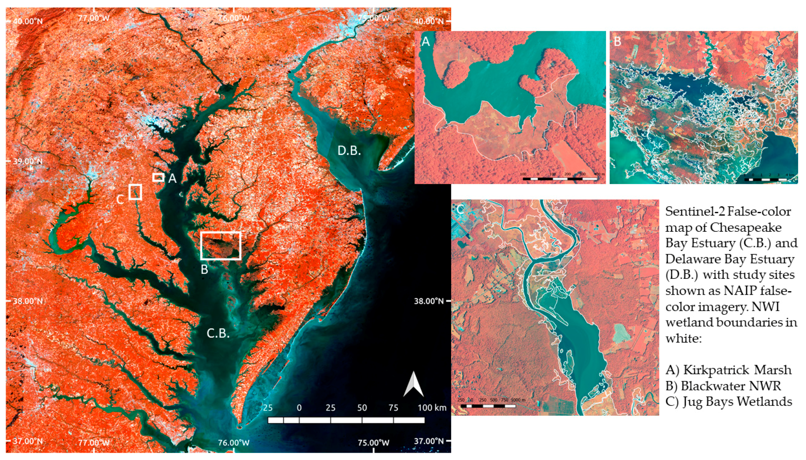
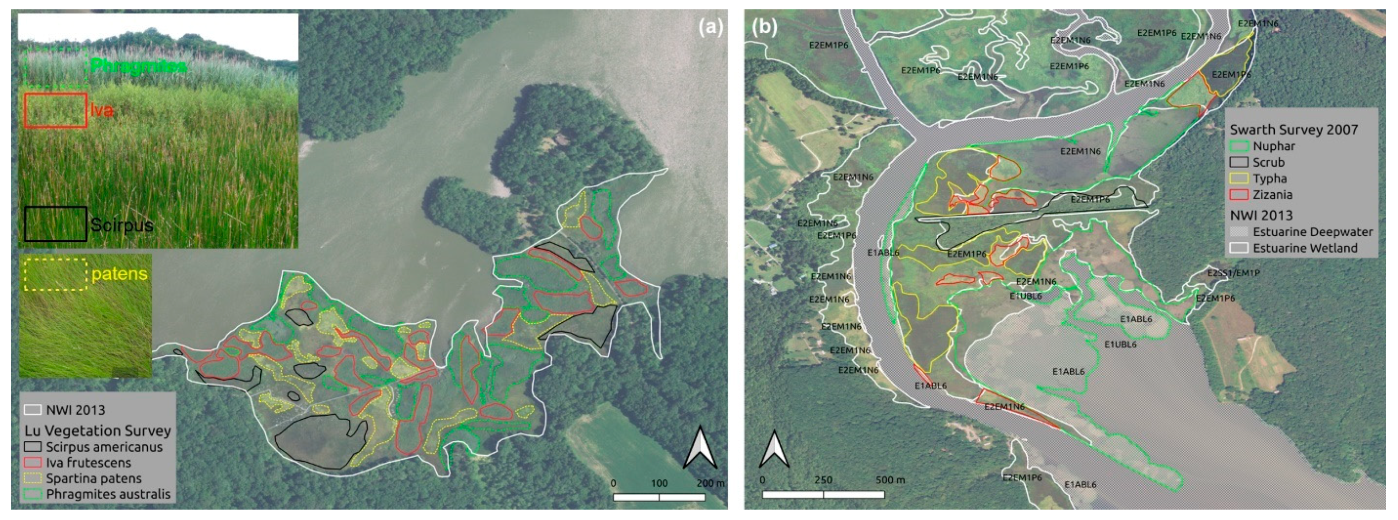
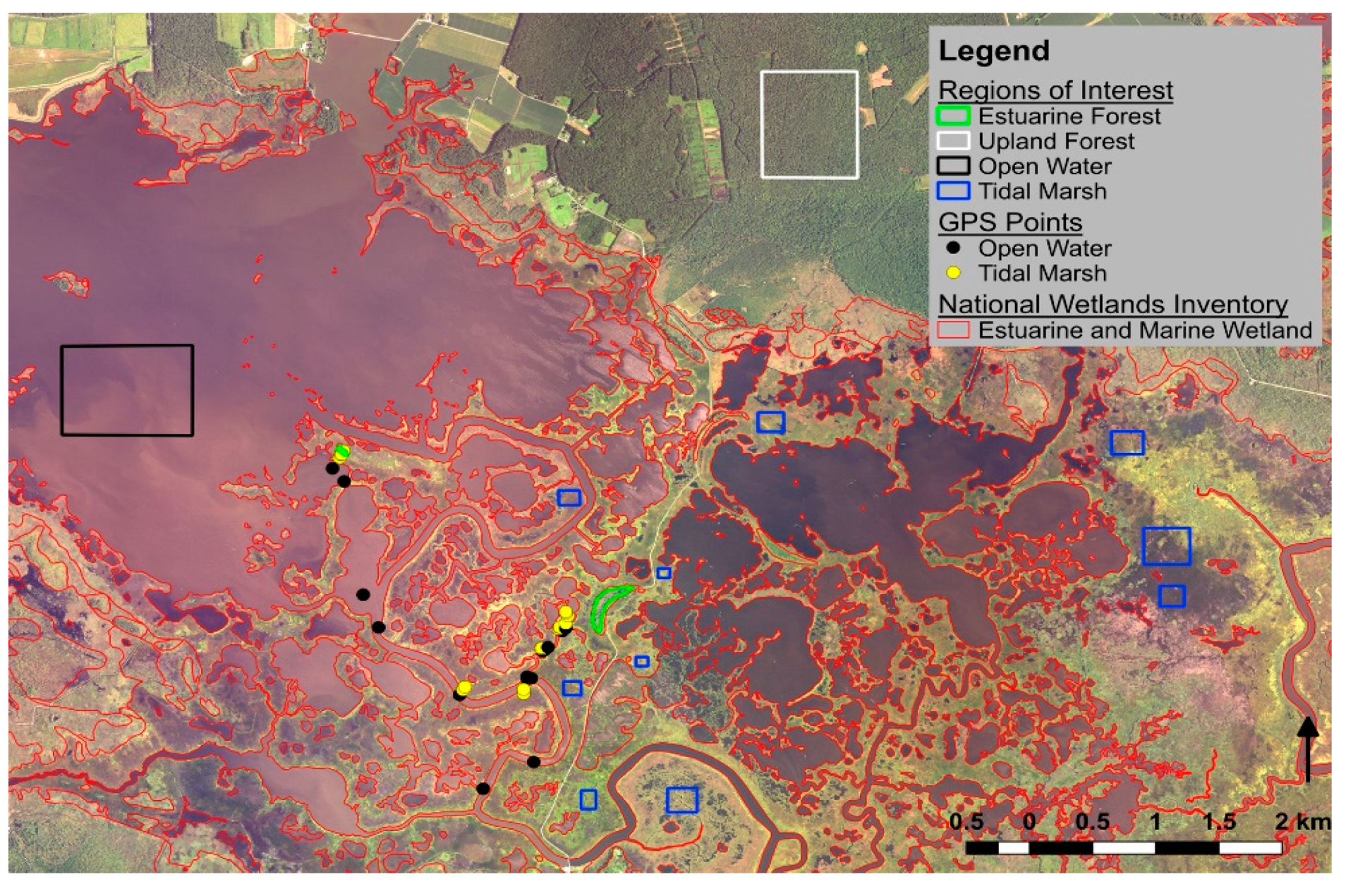
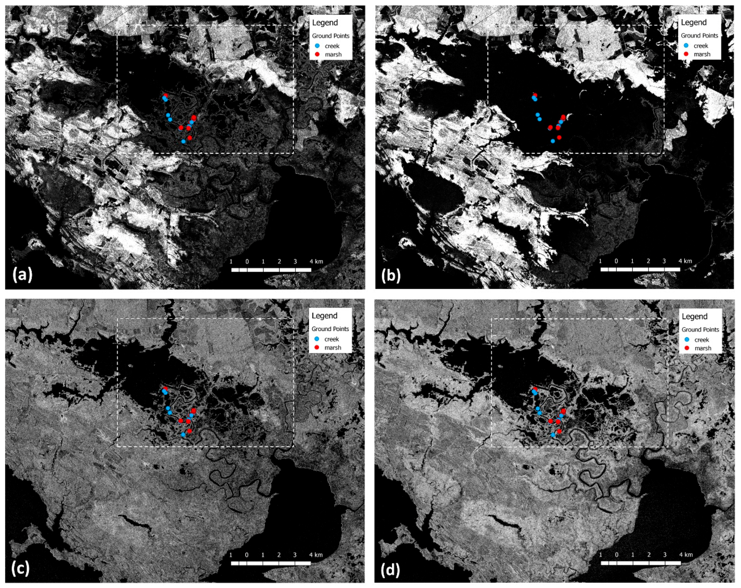
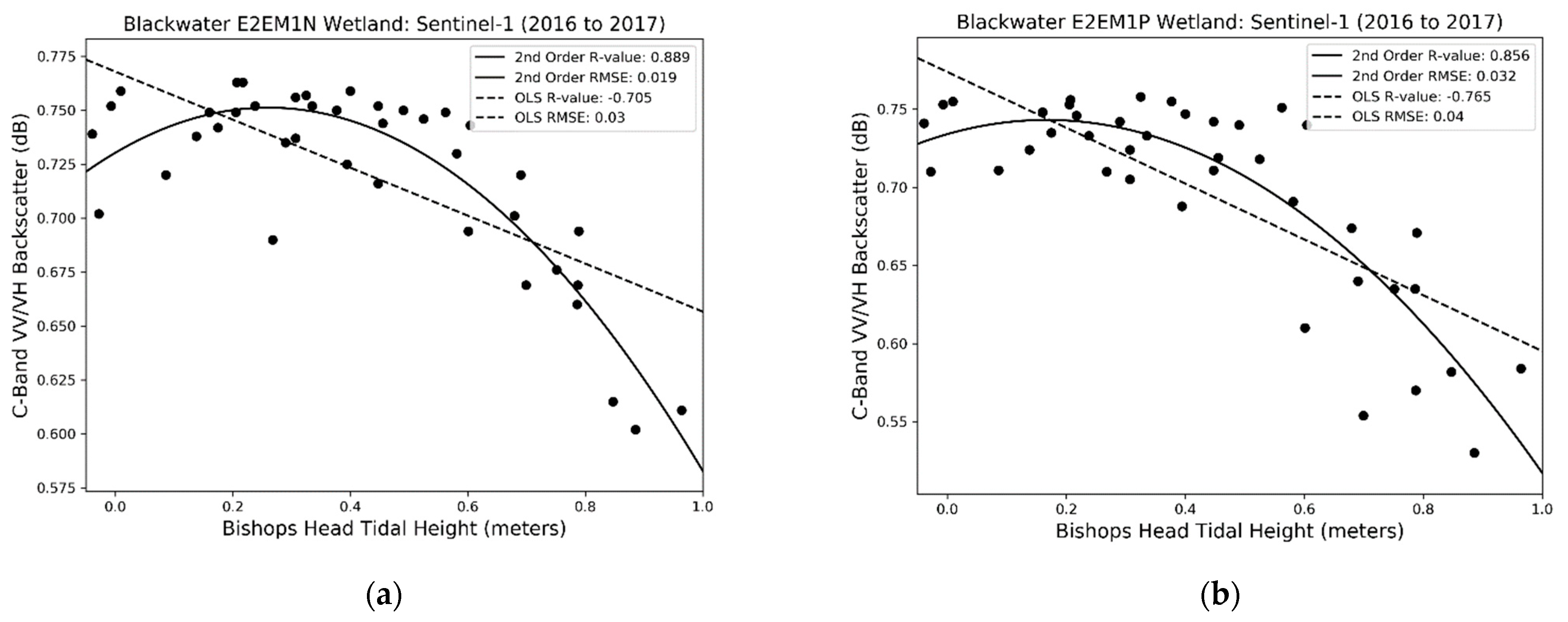
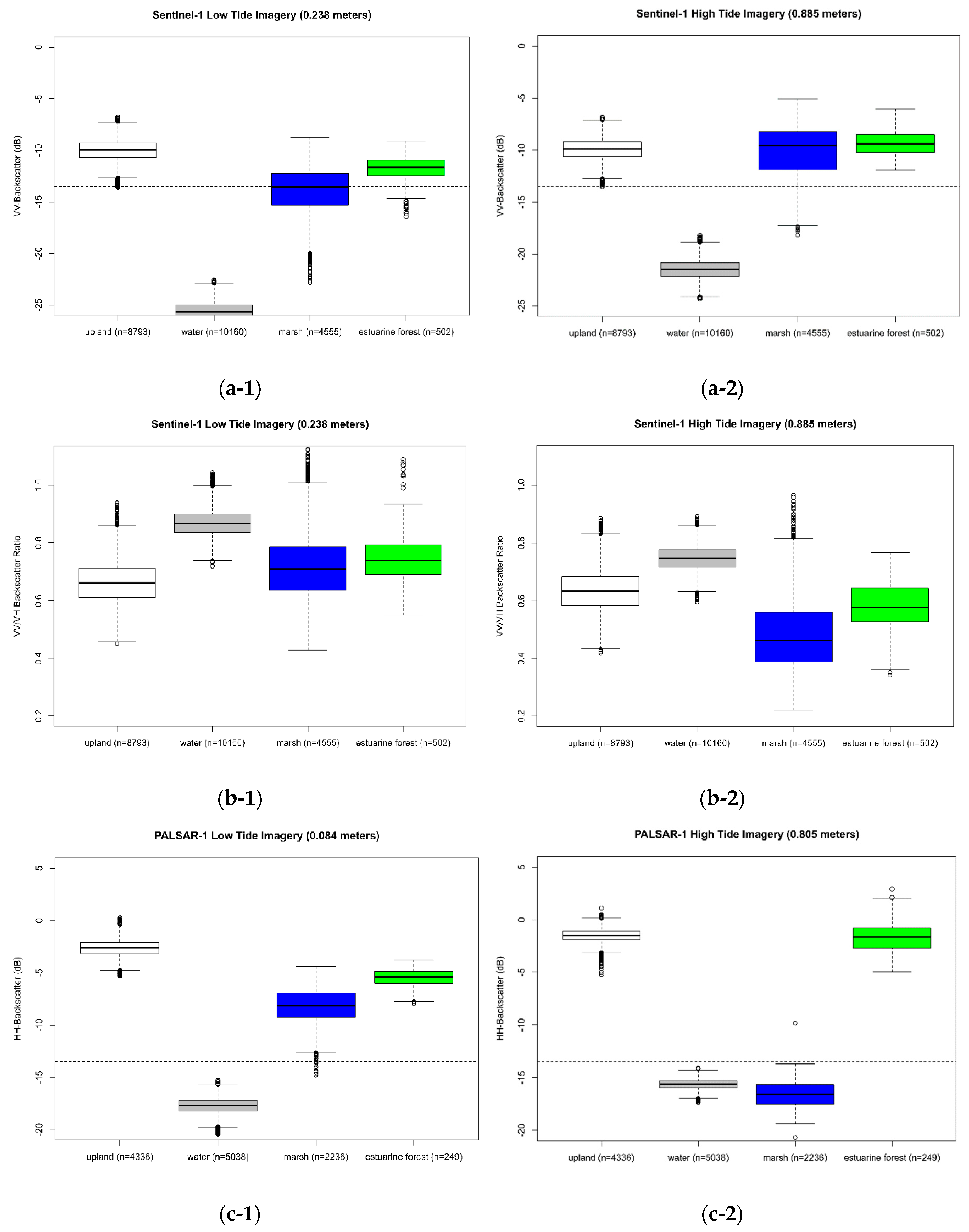
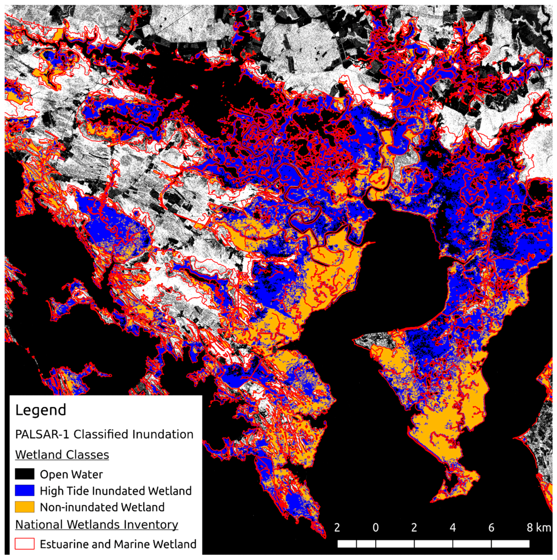
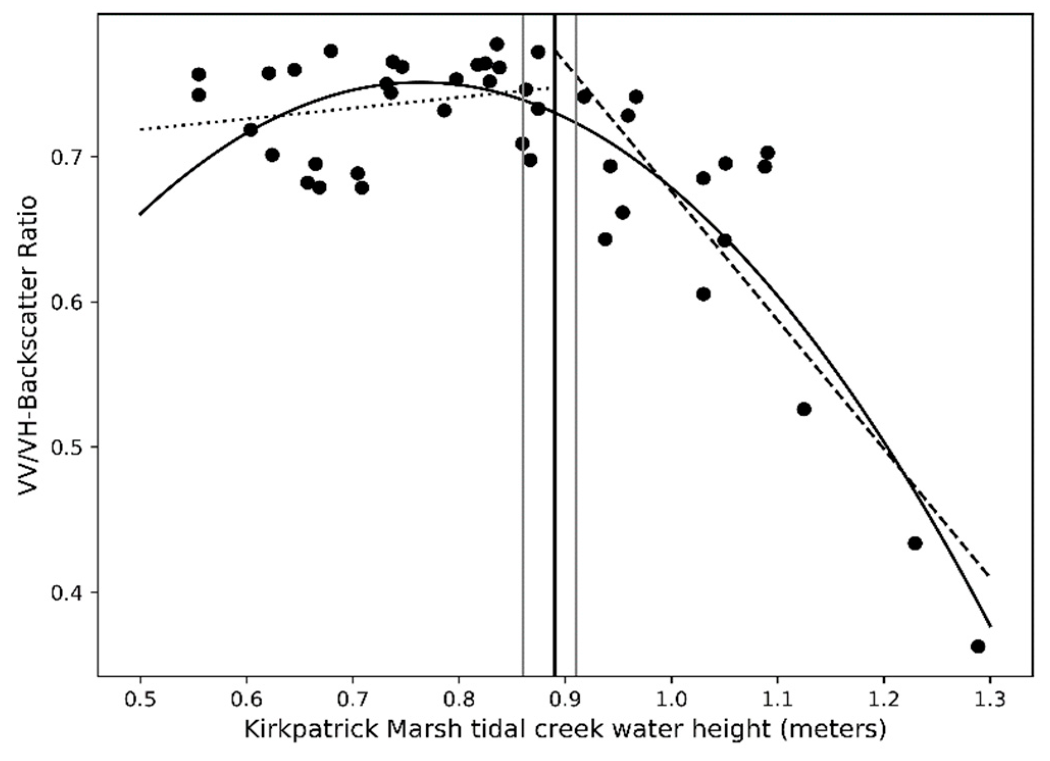
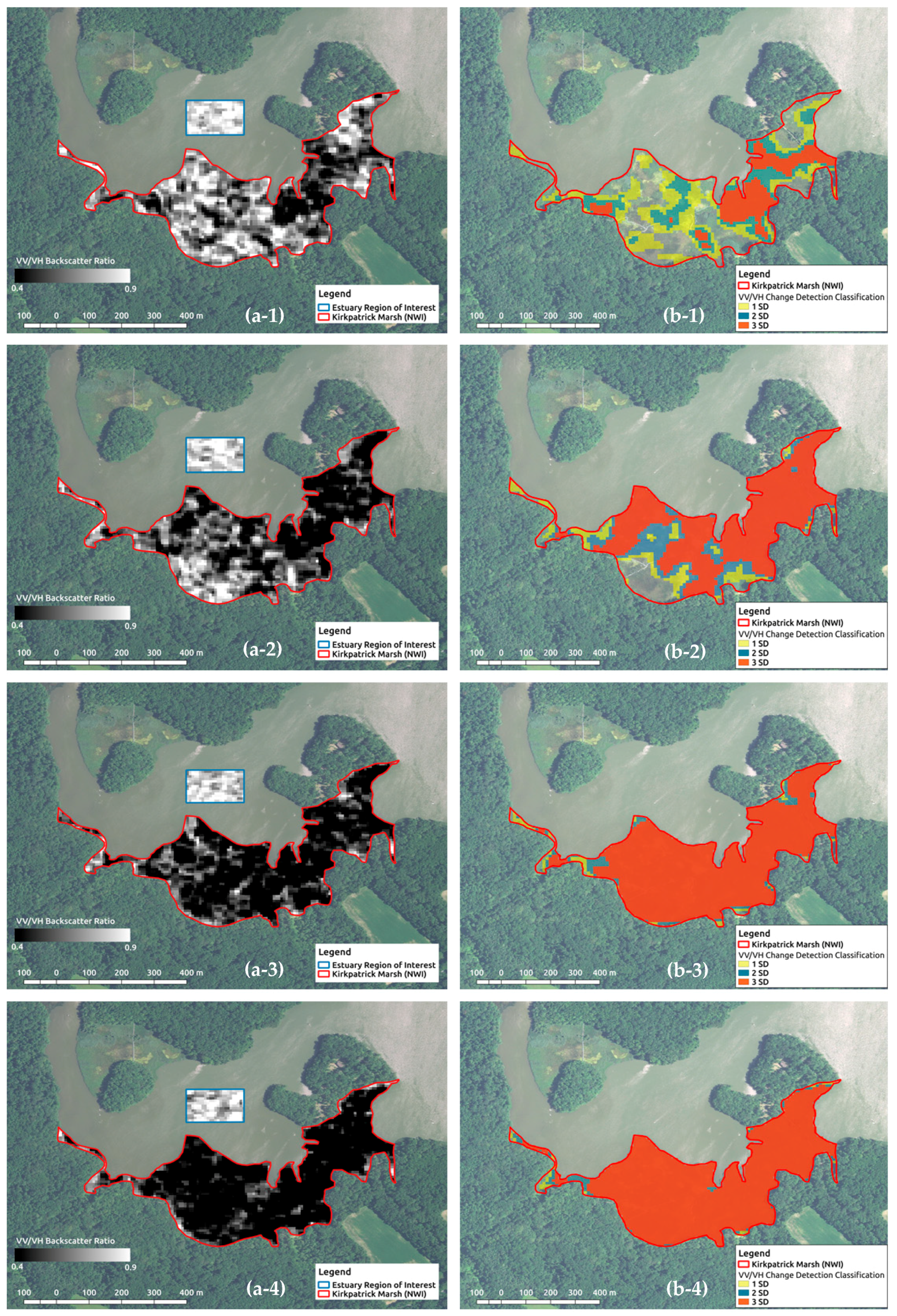
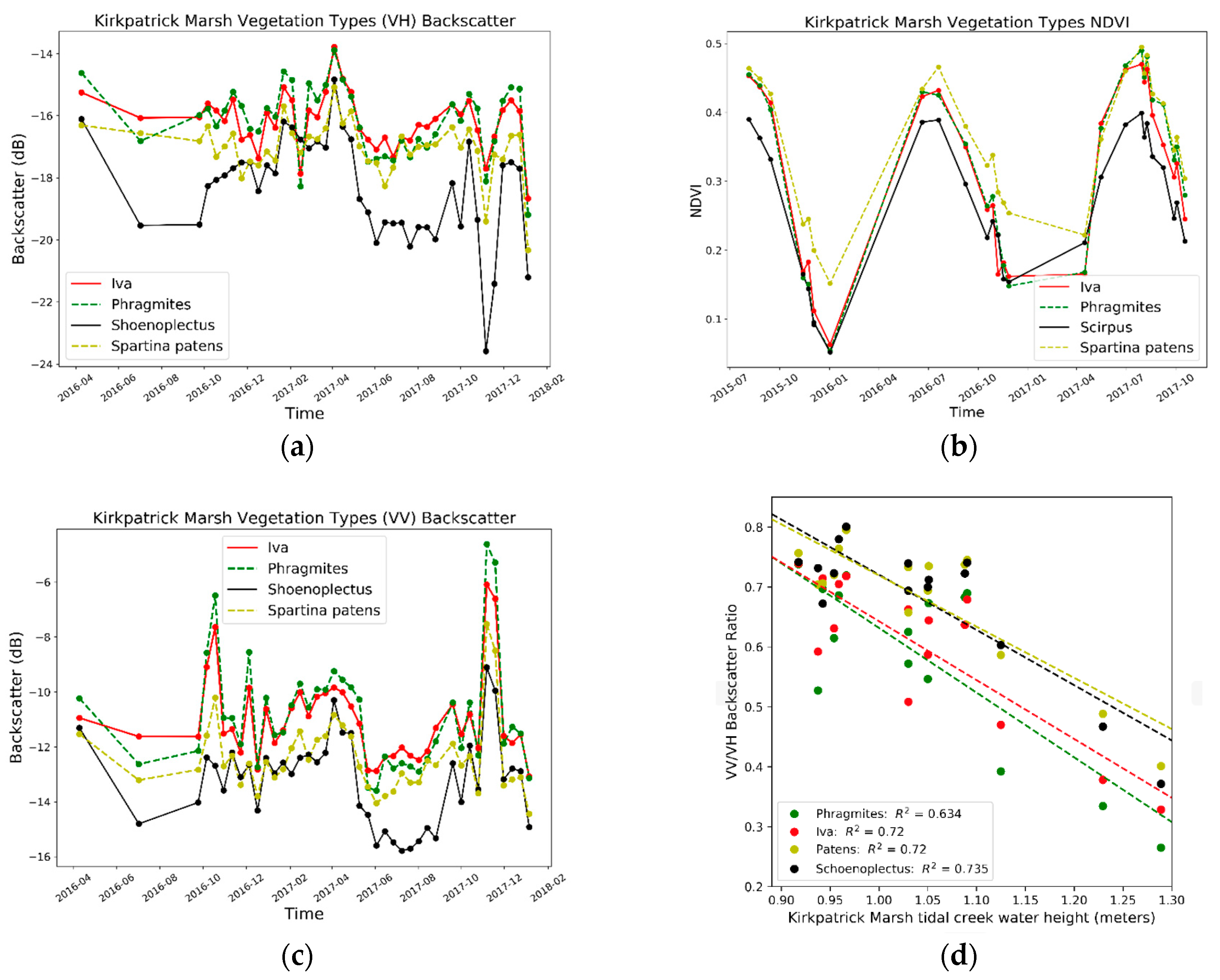
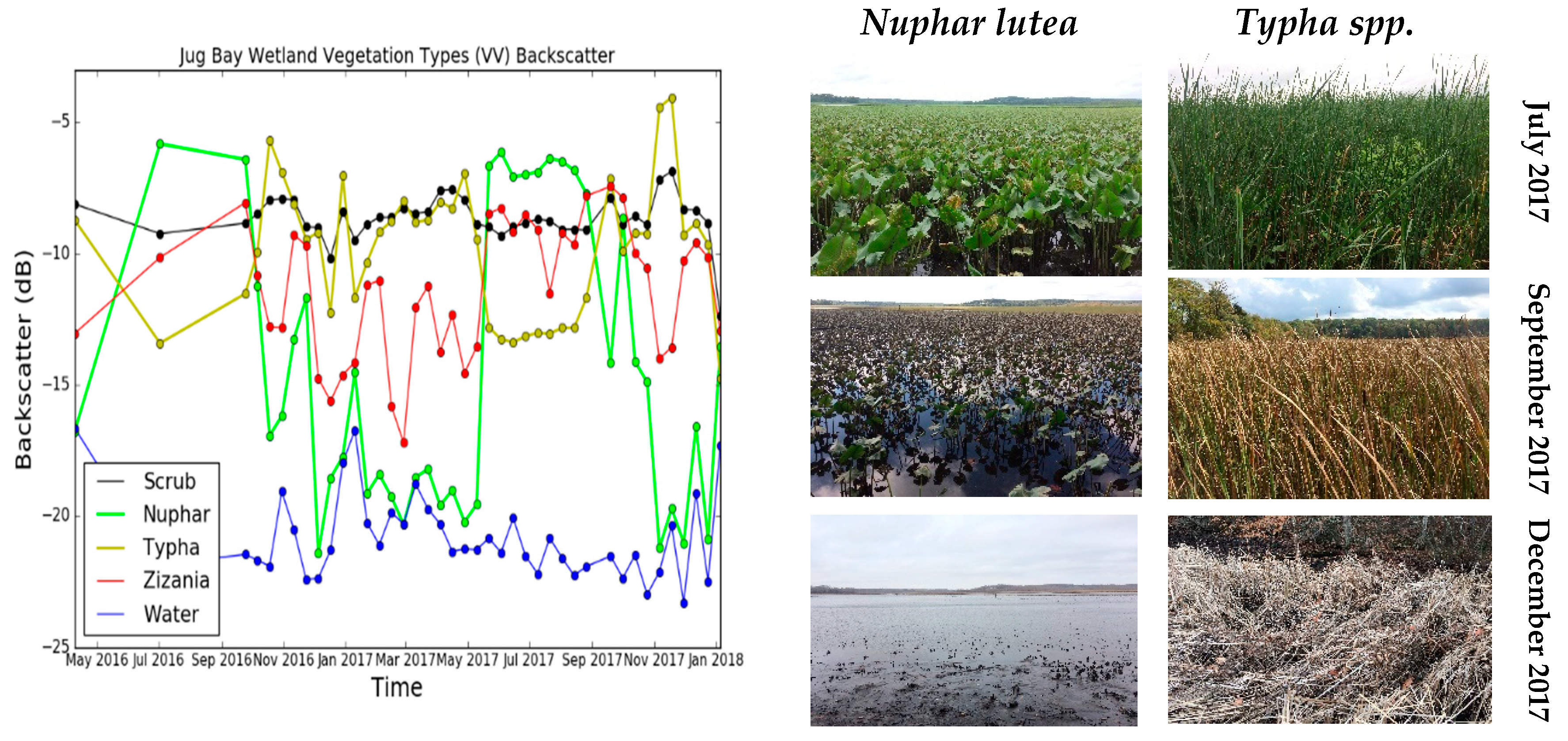
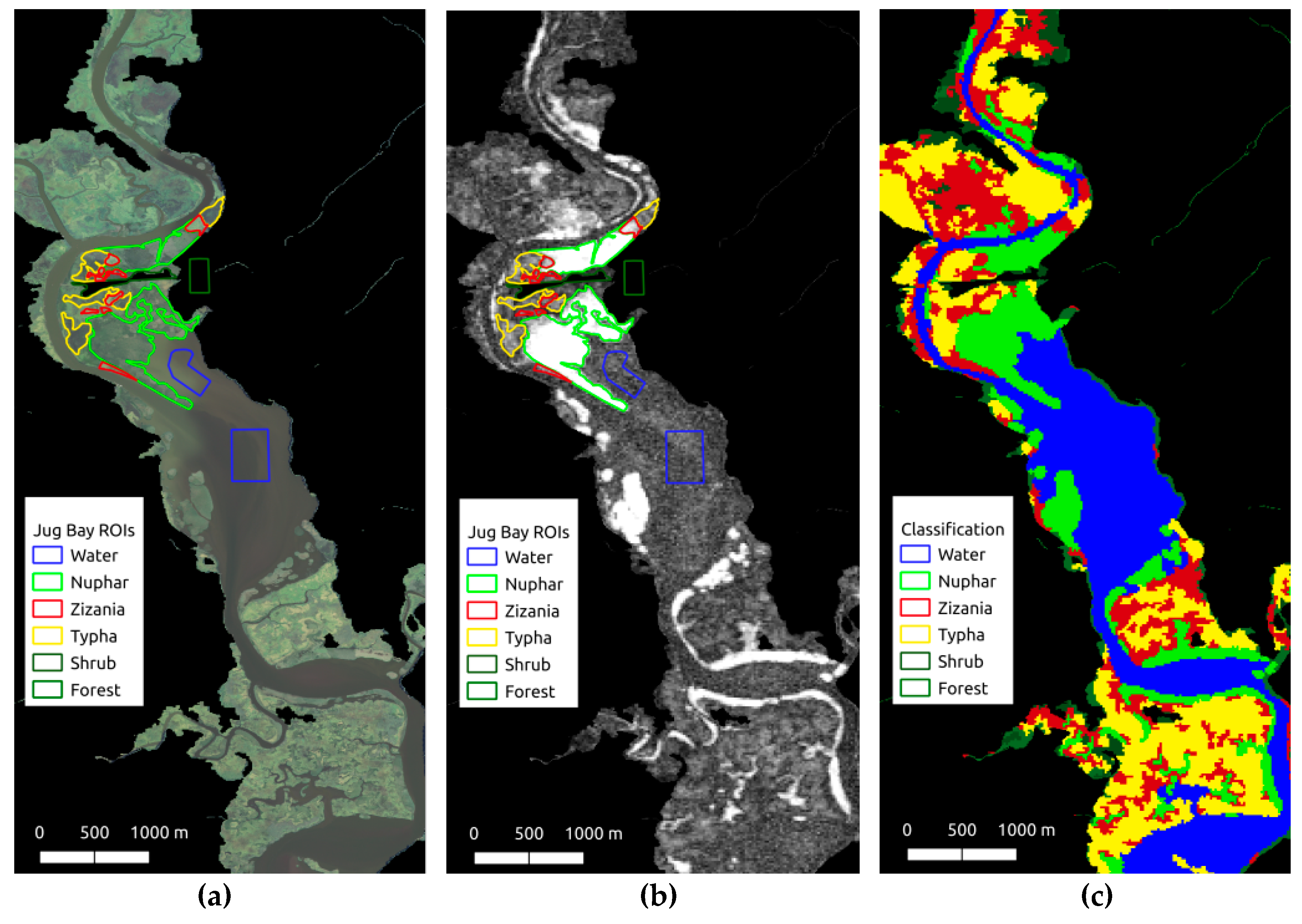
Table 1.
Adjusted Annapolis stage parameters for estimating tidal creek stage of Kirkpatrick Marsh.
| Date | n (minutes) | Max R-Value | Time Offset (minutes) | Height Offset (meters) |
|---|---|---|---|---|
| June 2016 | 6000 | 0.9911 | 34 | 0.4856 |
| October 2016 | 6000 | 0.9963 | 37 | 0.4769 |
| December 2016 | 6000 | 0.9912 | 32 | 0.4696 |
| Average | -- | -- | 34.33 | 0.4774 |
Table 2.
Description of input layers to regional scale random forest classification.
| Layer in GEE Stack | Description | Rationale | Example |
|---|---|---|---|
| vv_mean | Sentinel-1 VV 2017 annual mean | Decreases SAR speckle noise while preserving resolution, | Jug Bay |
| vh_mean | Sentinel-1 VH 2017 annual mean | captures central backscatter tendency | |
| vv_sd | Sentinel-1 VV 2017 annual standard deviation | Provides separability between high annual temporal variability | Jug Bay |
| vh_sd | Sentinel-1 VH 2017 annual standard deviation | emergent estuarine wetlands and other landcover | |
| vv_tidal_diff | Sentinel-1 VV tidal difference (Fall 2017) | Captures tidal variability in emergent estuarine systems presumably absent from other landcover | Blackwater, Kirkpatrick |
| vh_tidal_diff | Sentinel-1 VH tidal difference (Fall 2017) | ||
| vvvh_tidal_diff | Sentinel-1 VV/VH tidal difference (Fall 2017) | ||
| hh | PALSAR-2 HH 2017 annual mosaic | Provides biomass-based backscatter separability between | Blackwater |
| hv | PALSAR-2 HV 2017 annual mosaic | between emergent and forested wetlands | |
| summer_tvi | Landsat 8 TVI (Summer 2017) | Captures wetland vegetation phenology (three seasons help separate emergent wetlands from crops); more biomass | Kirkpatrick |
| fall_tvi | Landsat 8 TVI (Fall 2017) | separate emergent wetlands from crops); more biomass | |
| winter_tvi | Landsat 8 TVI (Winter 2017) | separability than NDVI | |
| summer_ndvi | Landsat 8 NDVI (Summer 2017) | Captures wetland vegetation phenology (three seasons help separate emergent wetlands from crops) | Kirkpatrick |
| fall_ndvi | Landsat 8 NDVI (Fall 2017) | ||
| winter_ndvi | Landsat 8 NDVI (Winter 2017) | ||
| summer_mndwi | Landsat 8 mNDWI (Summer 2017) | Captures fractional surface water in sparsely vegetated wetlands | Blackwater |
| fall_mndwi | Landsat 8 mNDWI (Fall 2017) | ||
| winter_mndwi | Landsat 8 mNDWI (Winter 2017) | ||
| elevation | SRTM DEM | Estuarine emergent wetlands close to sea-level | Sites low elevation |
| slope | SRTM DEM Gradient |
Table 3.
Pearson’s correlation (R-value) for Sentinel-1A (S1) and Sentinel-2A (S2) values and Bishop’s Head tidal stage for the ordinary least squares (OLS) fit and polynomial (Poly) fit.
Table 3.
Pearson’s correlation (R-value) for Sentinel-1A (S1) and Sentinel-2A (S2) values and Bishop’s Head tidal stage for the ordinary least squares (OLS) fit and polynomial (Poly) fit.
| NWI Class | S1-VH OLS | S1-VH Poly | S1-VV OLS | S1-VV Poly | S1-VV/VH OLS | S1-VV/VH Poly | S2-NDWI OLS | S2-NDWI Poly | S2-mNDWI OLS | S2-mNDWI Poly | Total Area (km2) |
|---|---|---|---|---|---|---|---|---|---|---|---|
| E2EM1N | −0.638 | 0.757 | 0.374 | 0.575 | −0.705 | 0.889 | 0.314 | 0.378 | 0.460 | 0.468 | 12.01 |
| E2EM1P | −0.689 | 0.761 | 0.581 | 0.666 | −0.765 | 0.856 | 0.352 | 0.393 | 0.471 | 0.515 | 284.40 |
| E2EM1P6 | −0.450 | 0.541 | 0.368 | 0.378 | −0.530 | 0.567 | 0.192 | 0.283 | 0.001 | 0.235 | 3.70 |
| E2EM1Pd | −0.646 | 0.725 | 0.457 | 0.539 | −0.684 | 0.772 | 0.407 | 0.412 | 0.560 | 0.669 | 15.38 |
| E2SS4P | −0.189 | 0.422 | 0.395 | 0.403 | −0.456 | 0.457 | 0.047 | 0.303 | −0.065 | 0.080 | 13.92 |
| E2FO4P | −0.089 | 0.357 | 0.360 | 0.381 | −0.401 | 0.401 | 0.006 | 0.236 | 0.108 | 0.142 | 24.63 |
Table 4.
Pearson’s correlation (R-value) for Sentinel-1A and Sentinel-2A values for the full tidal range (polynomial only) and above-bankfull depth (ABD) for Kirkpatrick Marsh tidal creek water level.
Table 4.
Pearson’s correlation (R-value) for Sentinel-1A and Sentinel-2A values for the full tidal range (polynomial only) and above-bankfull depth (ABD) for Kirkpatrick Marsh tidal creek water level.
| Imagery Type | Full Poly | OLS (ABD) | Poly (ABD) | n (ABD) |
|---|---|---|---|---|
| S1-VH | 0.326 | −0.478 | 0.572 | 13 |
| S1-VV | 0.790 | 0.819 | 0.859 | 13 |
| S1-VV/VH | 0.897 | −0.868 | 0.917 | 13 |
| S2-mNDWI | 0.280 | 0.335 | -- | 4 |
| S2-NDWI | 0.473 | −0.514 | -- | 4 |
Table 5.
Jug Bay random forest classification confusion matrix for SAR-only classification. Diagonal matches between observed (Reference) and predicted (Classification) classes are bolded.
Table 5.
Jug Bay random forest classification confusion matrix for SAR-only classification. Diagonal matches between observed (Reference) and predicted (Classification) classes are bolded.
| Classification | ||||||||
|---|---|---|---|---|---|---|---|---|
| Water | Nuphar | Zizania | Typha | Shrub | Forest | Producer’s Accuracy (%) | ||
| Reference | Water | 495 | 0 | 0 | 0 | 0 | 0 | 100.00 |
| Nuphar | 0 | 464 | 31 | 2 | 0 | 0 | 93.36 | |
| Zizania | 0 | 17 | 469 | 14 | 5 | 0 | 92.87 | |
| Typha | 0 | 1 | 14 | 481 | 9 | 2 | 94.87 | |
| Shrub | 0 | 1 | 6 | 10 | 471 | 5 | 95.54 | |
| Forest | 0 | 0 | 0 | 0 | 3 | 480 | 99.38 | |
| User’s Accuracy (%) | 100.00 | 96.07 | 90.19 | 94.87 | 96.52 | 98.56 | ||
| Overall Accuracy % | ||||||||
| 95.97 |
Table 6.
Jug Bay random forest classification confusion matrix for SAR-optical-DEM classification.
| Classification | ||||||||
|---|---|---|---|---|---|---|---|---|
| Water | Nuphar | Zizania | Typha | Shrub | Forest | Producer’s Accuracy (%) | ||
| Reference | Water | 500 | 0 | 0 | 0 | 0 | 0 | 100.00 |
| Nuphar | 1 | 481 | 19 | 6 | 0 | 1 | 94.69 | |
| Zizania | 0 | 8 | 477 | 5 | 3 | 0 | 96.75 | |
| Typha | 0 | 1 | 10 | 483 | 10 | 0 | 95.83 | |
| Shrub | 0 | 0 | 0 | 9 | 491 | 0 | 98.20 | |
| Forest | 0 | 0 | 0 | 0 | 0 | 496 | 100.00 | |
| User’s Accuracy (%) | 99.80 | 98.16 | 94.27 | 96.02 | 97.42 | 99.80 | ||
| Overall Accuracy % | ||||||||
| 97.57 |
Table 7.
Jug Bay random forest layer importance assessment for SAR-only classification. Columns 2–7 represent the decrease in accuracy predicting a given class when removing the input layer (predictor) in column 1. For example, the removal of the VV_mean layer (σ0VV annual mean) decreased the accuracy by 0.2193 when classifying a given pixel as water. Thus, higher values of accuracy decrease represent layer importance. Columns 8–9 represent the decrease in accuracy for all classes and decrease in the Gini coefficient. Top three layer classification improvements for each vegetation/landcover class prediction (columns) are bolded.
| Layer Type | Water | Nuphar | Zizania | Typha | Shrub | Forest | Mean Decrease Accuracy | Mean Decrease Gini |
|---|---|---|---|---|---|---|---|---|
| VV_mean | 0.2193 | 0.0763 | 0.0942 | 0.0789 | 0.3221 | 0.1573 | 0.1573 | 216.4184 |
| VH_mean | 0.1671 | 0.0706 | 0.1209 | 0.1133 | 0.2701 | 0.2326 | 0.1618 | 258.9103 |
| VV_SD | 0.0019 | 0.2059 | 0.1683 | 0.1864 | 0.3489 | 0.4963 | 0.2331 | 319.5366 |
| VH_SD | 0.0004 | 0.0905 | 0.2567 | 0.0511 | 0.2171 | 0.3411 | 0.1588 | 200.7394 |
| VV_summer | 0.2306 | 0.0858 | 0.1430 | 0.1562 | 0.1402 | 0.1806 | 0.1559 | 273.6167 |
| VH_summer | 0.1981 | 0.0437 | 0.0859 | 0.1374 | 0.1381 | 0.2040 | 0.1340 | 226.1407 |
| VV_fall | 0.0406 | 0.0028 | 0.0693 | 0.0252 | 0.1007 | 0.1058 | 0.0571 | 99.9647 |
| VH_fall | 0.0112 | 0.0357 | 0.1531 | 0.0456 | 0.2795 | 0.1928 | 0.1190 | 194.1971 |
| VV_winter | 0.0223 | 0.2752 | 0.2119 | 0.1622 | 0.2436 | 0.2148 | 0.1884 | 316.4512 |
| VH_winter | 0.0191 | 0.2163 | 0.2981 | 0.1751 | 0.2679 | 0.3360 | 0.2186 | 365.0655 |
Table 8.
Jug Bay random forest layer importance assessment for SAR-optical-DEM classification.
| Layer Type | Water | Nuphar | Zizania | Typha | Shrub | Forest | Mean Decrease Accuracy | Mean Decrease Gini |
|---|---|---|---|---|---|---|---|---|
| VV_mean | 0.2189 | 0.1184 | 0.1087 | 0.1070 | 0.1862 | 0.0334 | 0.1288 | 219.2148 |
| VH_mean | 0.2468 | 0.1930 | 0.1906 | 0.1637 | 0.3262 | 0.0269 | 0.1910 | 328.2239 |
| VV_SD | 0.0150 | 0.2690 | 0.0967 | 0.1428 | 0.2534 | 0.0179 | 0.1331 | 236.3179 |
| VH_SD | 0.0028 | 0.1636 | 0.1873 | 0.1304 | 0.2292 | 0.0158 | 0.1215 | 189.5208 |
| VV_tidal_diff | 0.0002 | 0.0044 | 0.1148 | 0.1492 | 0.0166 | 0.0003 | 0.0475 | 79.6682 |
| VH_tidal_diff | 0.0004 | 0.0031 | 0.1957 | 0.0228 | 0.0181 | 0.0121 | 0.0415 | 71.2645 |
| VVVH_tidal_diff | 0.0002 | 0.0060 | 0.0429 | 0.0849 | 0.0123 | 0.0010 | 0.0245 | 44.7473 |
| HH | 0.0213 | 0.0034 | 0.0276 | 0.0101 | 0.0206 | 0.0007 | 0.0138 | 15.6724 |
| HV | 0.0019 | 0.0033 | 0.0378 | 0.0130 | 0.0204 | 0.0005 | 0.0127 | 16.6604 |
| summer_tvi | 0.0581 | 0.0417 | 0.1470 | 0.0880 | 0.0595 | 0.0256 | 0.0698 | 111.7885 |
| summer_ndvi | 0.0685 | 0.0502 | 0.1196 | 0.0666 | 0.1002 | 0.2178 | 0.1034 | 182.2881 |
| summer_mndwi | 0.2041 | 0.0604 | 0.1324 | 0.0817 | 0.0573 | 0.0613 | 0.0991 | 180.2152 |
| fall_tvi | 0.0140 | 0.0861 | 0.1052 | 0.0406 | 0.0556 | 0.0324 | 0.0558 | 85.8827 |
| fall_ndvi | 0.0379 | 0.0601 | 0.1414 | 0.0978 | 0.1428 | 0.2085 | 0.1146 | 192.8352 |
| fall_mndwi | 0.1262 | 0.1097 | 0.1422 | 0.1020 | 0.1038 | 0.0411 | 0.1041 | 184.5659 |
| winter_tvi | 0.0065 | 0.0325 | 0.0798 | 0.0477 | 0.0254 | 0.1041 | 0.0492 | 70.8000 |
| winter_ndvi | 0.0054 | 0.0212 | 0.0871 | 0.0444 | 0.0320 | 0.0529 | 0.0404 | 67.6125 |
| winter_mndwi | 0.0738 | 0.0049 | 0.0959 | 0.0436 | 0.0186 | 0.0337 | 0.0448 | 40.8471 |
| DEM | 0.0213 | 0.0386 | 0.0593 | 0.0559 | 0.0533 | 0.2899 | 0.0862 | 142.0544 |
| DEM_grad | 0.0014 | 0.0029 | 0.0199 | 0.0121 | 0.0175 | 0.0001 | 0.0090 | 13.8682 |
Table 9.
Regional scale random forest classification confusion matrix. Diagonal matches between observed (Reference) and predicted (Classification) classes are bolded.
Table 9.
Regional scale random forest classification confusion matrix. Diagonal matches between observed (Reference) and predicted (Classification) classes are bolded.
| Classification | |||||||||||||
|---|---|---|---|---|---|---|---|---|---|---|---|---|---|
| Water | Urban | Barren | Grass | Agriculture | Shrub | Upland Forest | Forested Wetland | Palustrine Emergent | Estuarine Emergent | Total | Producer’s Accuracy % | ||
| Reference | Water | 22172 | 80 | 263 | 37 | 51 | 2 | 75 | 51 | 87 | 260 | 23078 | 96.07 |
| Urban | 31 | 11261 | 637 | 1957 | 1061 | 50 | 449 | 164 | 61 | 105 | 15776 | 71.38 | |
| Barren | 502 | 1522 | 4473 | 650 | 1575 | 233 | 669 | 221 | 107 | 290 | 10242 | 43.67 | |
| Grass | 31 | 2410 | 208 | 4449 | 4835 | 696 | 3643 | 1031 | 65 | 78 | 17446 | 25.50 | |
| Agriculture | 11 | 764 | 290 | 1666 | 22852 | 220 | 1699 | 615 | 113 | 31 | 28261 | 80.86 | |
| Shrub | 16 | 311 | 106 | 1039 | 1486 | 2853 | 5059 | 1535 | 45 | 27 | 12477 | 22.87 | |
| Upland Forest | 28 | 494 | 100 | 1431 | 1415 | 1343 | 23427 | 3374 | 30 | 7 | 31649 | 74.02 | |
| Forested Wetland | 56 | 254 | 53 | 496 | 585 | 529 | 3662 | 10732 | 372 | 224 | 16963 | 63.27 | |
| Palustrine Emergent | 93 | 75 | 73 | 116 | 1009 | 83 | 171 | 550 | 5954 | 950 | 9074 | 65.62 | |
| Estuarine Emergent | 127 | 71 | 160 | 34 | 53 | 2 | 1 | 130 | 699 | 9993 | 11270 | 88.67 | |
| Total | 23067 | 17242 | 6363 | 11875 | 34922 | 6011 | 38855 | 18403 | 7533 | 11965 | |||
| User’s Accuracy % | 96.12 | 65.31 | 70.30 | 37.47 | 65.44 | 47.46 | 60.29 | 58.32 | 79.04 | 83.52 | Overall Accuracy % | ||
| 67.05 | |||||||||||||
Table 10.
Regional scale random forest layer importance assessment.
| LayerType | Water | Urban | Barren | Grass | Ag. | Shrub | U. Forest | W. Forest | Palustrine | Estuarine | Mean Decrease Accuracy | Mean Decrease Gini |
|---|---|---|---|---|---|---|---|---|---|---|---|---|
| vv | 0.286 | 0.027 | 0.026 | 0.000 | 0.040 | 0.006 | 0.051 | 0.063 | 0.038 | 0.092 | 0.071 | 6792.088 |
| vh | 0.282 | 0.020 | 0.074 | −0.003 | 0.112 | 0.020 | 0.103 | 0.127 | 0.069 | 0.116 | 0.104 | 10293.323 |
| vv_sd | 0.018 | 0.005 | 0.009 | −0.002 | 0.022 | 0.001 | 0.026 | 0.024 | 0.029 | 0.016 | 0.016 | 4621.997 |
| vh_sd | 0.007 | 0.017 | 0.016 | 0.002 | 0.075 | 0.016 | 0.038 | 0.042 | 0.048 | 0.036 | 0.032 | 7285.724 |
| vv_tidal_diff | 0.000 | 0.003 | 0.002 | 0.000 | 0.004 | 0.000 | 0.005 | 0.004 | 0.003 | 0.005 | 0.003 | 3740.538 |
| vh_tidal_diff | 0.000 | 0.002 | 0.001 | 0.000 | 0.005 | 0.000 | 0.005 | 0.003 | 0.003 | 0.010 | 0.003 | 3897.383 |
| vvvh_tidal_diff | 0.001 | 0.001 | 0.002 | 0.000 | 0.005 | 0.001 | 0.002 | 0.001 | 0.002 | 0.005 | 0.002 | 3669.585 |
| hh | 0.027 | 0.017 | 0.005 | −0.001 | 0.019 | 0.003 | 0.022 | 0.029 | 0.014 | 0.019 | 0.017 | 4689.331 |
| hv | 0.072 | 0.033 | 0.011 | 0.001 | 0.027 | 0.010 | 0.041 | 0.031 | 0.023 | 0.052 | 0.033 | 5633.296 |
| summer_tvi | 0.179 | 0.148 | 0.070 | 0.012 | 0.054 | 0.014 | 0.025 | 0.029 | 0.066 | 0.292 | 0.081 | 8488.662 |
| summer_ndvi | 0.184 | 0.237 | 0.133 | 0.023 | 0.028 | 0.026 | 0.094 | 0.167 | 0.102 | 0.268 | 0.117 | 11751.909 |
| summer_mndwi | 0.245 | 0.174 | 0.032 | 0.009 | 0.044 | 0.014 | 0.044 | 0.042 | 0.098 | 0.128 | 0.084 | 8987.405 |
| fall_tvi | 0.093 | 0.084 | 0.034 | 0.009 | 0.042 | 0.015 | 0.032 | 0.014 | 0.060 | 0.290 | 0.059 | 7603.245 |
| fall_ndvi | 0.148 | 0.170 | 0.092 | 0.020 | 0.036 | 0.039 | 0.078 | 0.066 | 0.095 | 0.235 | 0.091 | 11122.123 |
| fall_mndwi | 0.237 | 0.166 | 0.036 | 0.014 | 0.037 | 0.021 | 0.042 | 0.033 | 0.096 | 0.104 | 0.079 | 12343.496 |
| winter_tvi | 0.078 | 0.048 | 0.026 | 0.011 | 0.062 | 0.030 | 0.031 | 0.017 | 0.110 | 0.205 | 0.055 | 6736.456 |
| winter_ndvi | 0.349 | 0.081 | 0.063 | 0.010 | 0.034 | 0.073 | 0.046 | 0.043 | 0.090 | 0.072 | 0.090 | 8764.048 |
| winter_mndwi | 0.205 | 0.128 | 0.023 | 0.004 | 0.045 | 0.018 | 0.045 | 0.027 | 0.089 | 0.077 | 0.069 | 9277.989 |
| dem | 0.198 | 0.052 | 0.038 | 0.025 | 0.051 | 0.039 | 0.171 | 0.120 | 0.243 | 0.451 | 0.130 | 14884.806 |
| dem_grad | 0.274 | 0.008 | 0.011 | 0.000 | 0.006 | 0.001 | 0.029 | 0.005 | 0.008 | 0.016 | 0.045 | 4979.564 |
© 2019 by the authors. Licensee MDPI, Basel, Switzerland. This article is an open access article distributed under the terms and conditions of the Creative Commons Attribution (CC BY) license (http://creativecommons.org/licenses/by/4.0/).
Share and Cite
MDPI and ACS Style
Lamb, B.T.; Tzortziou, M.A.; McDonald, K.C. Evaluation of Approaches for Mapping Tidal Wetlands of the Chesapeake and Delaware Bays. Remote Sens. 2019, 11, 2366. https://0-doi-org.brum.beds.ac.uk/10.3390/rs11202366
AMA Style
Lamb BT, Tzortziou MA, McDonald KC. Evaluation of Approaches for Mapping Tidal Wetlands of the Chesapeake and Delaware Bays. Remote Sensing. 2019; 11(20):2366. https://0-doi-org.brum.beds.ac.uk/10.3390/rs11202366
Chicago/Turabian StyleLamb, Brian T., Maria A. Tzortziou, and Kyle C. McDonald. 2019. "Evaluation of Approaches for Mapping Tidal Wetlands of the Chesapeake and Delaware Bays" Remote Sensing 11, no. 20: 2366. https://0-doi-org.brum.beds.ac.uk/10.3390/rs11202366
Note that from the first issue of 2016, this journal uses article numbers instead of page numbers. See further details here.