A Review of the Applications of Remote Sensing in Fire Ecology


Department of Geography, Texas State University, San Marcos, TX 78666, USA
*
Author to whom correspondence should be addressed.
Remote Sens. 2019, 11(22), 2638; https://0-doi-org.brum.beds.ac.uk/10.3390/rs11222638
Submission received: 5 October 2019
/
Revised: 6 November 2019
/
Accepted: 7 November 2019
/
Published: 12 November 2019
(This article belongs to the Special Issue Remote Sensing Approaches to Biogeographical Applications)
Abstract
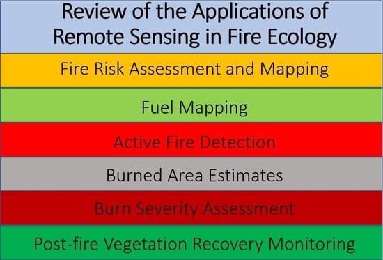
:Wildfire plays an important role in ecosystem dynamics, land management, and global processes. Understanding the dynamics associated with wildfire, such as risks, spatial distribution, and effects is important for developing a clear understanding of its ecological influences. Remote sensing technologies provide a means to study fire ecology at multiple scales using an efficient and quantitative method. This paper provides a broad review of the applications of remote sensing techniques in fire ecology. Remote sensing applications related to fire risk mapping, fuel mapping, active fire detection, burned area estimates, burn severity assessment, and post-fire vegetation recovery monitoring are discussed. Emphasis is given to the roles of multispectral sensors, lidar, and emerging UAS technologies in mapping, analyzing, and monitoring various environmental properties related to fire activity. Examples of current and past research are provided, and future research trends are discussed. In general, remote sensing technologies provide a low-cost, multi-temporal means for conducting local, regional, and global-scale fire ecology research, and current research is rapidly evolving with the introduction of new technologies and techniques which are increasing accuracy and efficiency. Future research is anticipated to continue to build upon emerging technologies, improve current methods, and integrate novel approaches to analysis and classification.
1. Introduction
Wildfires significantly impact environments and communities around the world by changing vegetation composition [1], altering soil characteristics lasting years after the fire [2,3], and modifying hydrologic regimes by increasing runoff and decreasing soil infiltration [4,5]. Wildfires also cause losses in human life and property. While some of these changes to local environments are desirable from an ecological perspective, the destructive and harmful consequences of wildfires are generally considered undesirable and require mitigation.
It is expected that fire regimes will be altered by the changing climate, with several studies generally forecasting increased areas susceptible to wildfires, increased intensity of future fires, and an increase in fire occurrence in areas already prone to fire events [6,7,8,9,10,11,12]. Increased wildfire activity can act as a driver of climate change via the increased release CO2, soot, and aerosols during combustion, and through the removal of vegetation which would otherwise have served as a CO2 sink. If the prediction of increasing frequency and intensity of fire events holds true, then these fires will contribute to the global trend of rising temperatures, which creates positive feedback by increasing the likelihood of wildfires, especially in areas that possess favorable environmental and climactic conditions for wildfire ignition and spread.
Remote sensing provides a means for analyzing conditions and monitoring changes over large geographic extents, making it useful for studies in fire ecology. Remote sensing systems provide biophysical measurements of the ground conditions prior to and post-fire. These measurements have been used to assist in fire risk mapping [13,14,15], fuel mapping [16,17,18,19,20], active fire detection [21,22,23,24,25], burned area estimates [26,27,28], assessing burn severity [29,30,31,32], and monitoring vegetation recovery [33,34,35]. The most commonly used remote sensing systems for fire ecology research are space-based, multispectral sensors (Table 1). These sensors image the Earth at regular intervals, providing data on the amount of energy reflected in multiple regions of the electromagnetic spectrum.
Recent advancements in remote sensing technology have facilitated new approaches to studying fire ecology. Light detection and ranging (lidar) has rapidly increased in popularity in nearly every type of remote sensing research, including fire ecology, over the last two decades. Lidar systems generate 3-D models based on ranges derived from pulsed lasers of light. Lidar data are used to create highly accurate digital terrain models (DTMs) [64,65], model forest stands in 3-D [66,67,68], and aid more traditional multispectral methods in classification [69,70], all of which are useful for fire ecologists. Of particular interest for fire managers, lidar has been incorporated into the mapping of surface fuels [20,71,72], assessing burn severity [48,73,74], and monitoring vegetation recovery [75,76], due to its ability to accurately measure vegetation structural properties.
Unmanned aerial system (UAS) technologies have recently been used to acquire hyperspatial imagery, construct orthomosaics, and generate 3-D models using structure-from-motion (SfM). SfM is a newer methodology which incorporates the use of photogrammetric techniques to construct 3-D ‘point clouds’ from a series of overlapping images. Although UAS-based research is an emerging technology, the data have been used for monitoring post-fire vegetation recovery [77], fire severity [78], and fire detection [79]. UAS technology provides the means for rapid and cost-effective data acquisition necessary for fire ecology research by providing timely multispectral measurements and 3-D models of terrain and vegetation structure.
The purpose of this paper is to outline the ways remote sensing is currently being used in fire ecology research. Remote sensing is a broad term which can include numerous types of sensors, so for the purpose of this review, remote sensing is limited to imagery acquired by orbital sensors, lidar systems, and UASs. The paper examines research in several broad categories, which include fire risk modeling, fuel mapping, active fire detection, burned area estimates, burn severity assessments, and monitoring vegetation recovery. Within each category, current research trends and case examples are presented. Each category’s discussion is broken down by research related to orbital multispectral sensors, lidar, and UAS technologies. The final section comments on future research trends. The goal of this paper is to provide the reader with a snapshot of the current applications of remote sensing technologies and techniques in the field of fire ecology.
2. Fire Risk Assessment and Mapping
Fire risk mapping is used to predict where ignition events will occur as well as how the resulting wildfire will propagate and the potential damages that may result from a fire occurrence [13,80,81]. To assess fire risk, variables which increase the probability of fire occurrence are used to map fire hazard/danger. This is accomplished through two primary methods: (i) point-wise meteorological data-based operating systems and (ii) the use of remote sensing technologies and geographic information systems (GIS). The former method, which assesses fire danger, has four main operating systems used around the world: Wildland Fire Assessment System (WFAS), Fire Weather Index (FWI), McArthur’s Forest Fire Danger Rating System (FFDRS), and Russian Nesterov Index. These systems use meteorological data such as temperature, precipitation, humidity, and wind speed to assess fire danger over large geographic regions. However, these systems suffer from several limitations including input data being limited to the point distribution of data collection stations and the need for interpolation to generate fire danger maps. Due to the ability to obtain continuous data for an area, the remote sensing/GIS approach is recognized as an effective alternative for the creation of fire risk maps [13,14,15].
Fire hazard differs from fire danger as it does not include a meteorological component in the assessment [82]. Instead, fire hazard maps use measurements of environmental factors, such as fuel conditions and topography, and may also include proximity to human settlement/infrastructure to identify areas at risk of fire occurrence [13,83,84,85]. Fire risk mapping builds upon fire hazard maps by adding variables which assess vulnerability into the assessment [82,83]. Fire risk maps may also include dynamic variables such as weather and vegetation conditions. The result is a map which displays varying degrees of fire risk ranging from very low to very high (Figure 1). These maps can be broken into two broad categories: long-term and short-term. Long-term (seasonal) fire risk maps generally map risk using inputs which do not vary greatly over time such as vegetation type, human settlements, and topography [14,86]. Short-term fire risk maps normally provide risk estimates that are only appropriate for a short period (days‒weeks) after their creation. Short-term fire risk maps use many of the same inputs as long-term fire risk maps but also include variables that are continuously changing such as fuel moisture content, weather conditions and vegetation conditions [14,86]. These maps are used by land managers to reduce the risk of eventual fire events through controlled burns and mechanical thinning, preparation of evacuation routes, and allocation of firefighting resources.
Studies that use remote sensing for fire risk mapping go back decades and use similar variables, but they implement these variables in diverse ways and in different environments. Before fire risk mapping, the focus of research was on fire hazard mapping, which is more related to fuel sources. Chuvieco and Congalton [13] used remote sensing and GIS to identify areas of varying fire hazard potentials in a Mediterranean environment primarily composed of Aleppo Pine (Pinus halepensi) on the southeastern coast of Spain. They used Landsat TM classified vegetation, elevation data obtained from topographic maps, and trail and road locations. Validation of this long-term fire hazard map was performed by comparing a pre-fire risk potential map to the results of a 1985 fire event. Fire hazard methods have since developed into fire risk mapping which includes vulnerability in the assessment and can also incorporate dynamic variables such as fuel moisture conditions.
In recent fire risk assessment studies, remote sensing is used primarily to classify land cover, provide elevation data, assess vegetation conditions, and validate proposed risk assessments. Land cover plays an important role in evaluating the risk of a given area to fire events as it is related to fuel types and characteristics [80]. This makes accurate classification of land cover essential for identifying areas of high risk. But classification alone is limited, as it does not provide data on the current conditions of the potential fuel sources. As such, vegetation indices such as the Normalized Difference Moisture Index (NDMI) and Normalized Difference Vegetation Index (NDVI) are commonly incorporated into fire risk models [13,14,15]. These indices are used to identify vegetation conditions which are most susceptible to an ignition or spreading event and to model fuel loads. These conditions change rapidly, requiring frequent updates when used for mapping fire risk dynamically. Topographic data are important as slope, aspect and elevation all influence the risk of an area to fire ignition and/or spread [13,14,85]. Active fire and burn severity data are commonly used to test the accuracy of fire risk assessments, with the expectation that fire events will most commonly occur in areas of higher risk [13,14,87].
Modern studies have built upon the work of Chuvieco and Congalton [13], incorporating newer sensors and indices, modern land cover classifications, additional ancillary data, and variables to assess vulnerability [14,15,84,87]. Adab et al. [14] created a new combined fire risk index termed the Hybrid Fire Index (HFI). The variables used in this study include the NDMI, elevation, slope, aspect, distance from roads, and proximity to settlement. The inputs were reclassified based on how each influenced fire risk, and multicriteria analysis was used to create a fire risk map for a region with a Mediterranean climate in northwestern Iran. When assessed using the receiver operating characteristic and Moderate Resolution Imaging Spectroradiometer (MODIS) active fire data, the map was shown to have an accuracy of 76.7%. Chuvieco et al. [88] presented a method for evaluating fire risk which may be applicable at various spatial scales. Multiple inputs were used to create synthetic indices for living/dead fuel moisture content, lightning probability, fire propagation, human influence, socioeconomic vulnerability, and ecological vulnerability. The study found that significant differences in the risk rating existed between areas affected by fires and those which were not.
Many recent studies have focused on the use of empirical equations or simulated fire spread to estimate fire risk [89,90,91,92]. This newer approach uses remote sensing data as some of the inputs for fire risk mapping, but also includes other factors such as fuel distribution, historical wildfire spread, wind direction, and weather conditions. An example of a commonly used model for simulating fire growth is FARSITE [93]. The inputs for FARSITE are elevation, slope, aspect, surface fuel conditions, canopy cover, canopy height, crown base height, crown bulk density, min/max temperatures, humidity, precipitation, windspeed, wind direction, and cloud cover. FARSITE then uses existing fire behavior models to simulate how the fire will grow and behave. The addition of these other inputs and the use of statistical models and simulations allow for fire risk maps which are of higher spatial resolution and which better account for the complexity of estimating fire risk.
Multispectral based remote sensing provides fundamental inputs for the mapping of fire risk [14,15,85,87,94]. While spectral data cannot provide risk estimates alone, products derived from this data are important variables for risk assessment, making remote sensing a key factor for performing these assessments. When combined with other spatial data, this information allows researchers and land managers to effectively assess the risk of fire ignition and propagation for various spatial extents.
Selecting appropriate sensors for fire risk mapping is important because of the different spatial and temporal resolution requirements for long- and short-term mapping. Long-term fire risk maps do not require a high temporal resolution as they are not frequently updated. Sensors with high to moderate spatial resolutions (<100 m), such as the sensors onboard the Landsat series, Sentinel-2, and Advanced Spaceborne Thermal Emission and Reflection Radiometer (ASTER) are capable of providing data for mapping the required inputs for long-term fire risk maps. A spatial resolution of 30 m or less is generally seen as an appropriate spatial resolution for classifying inputs such as landcover/land use and so is appropriate for long-term risk maps. For short-term fire risk mapping a higher temporal resolution is required (daily‒weekly). While it is possible to map the required variables with the previously mentioned sensors, the low temporal resolution limits the user’s ability to rapidly update dynamic conditions. As a result, it may be more appropriate to use coarser spatial resolution sensors (>100 m) which have more frequent revisit intervals, such as MODIS or the sensors aboard Sentinel-3. The sensors onboard the recently launched Sentinel-2 satellites have a revisit interval of five days, which makes these systems capable of weekly updates to fire risk maps at moderate spatial resolutions (10‒20 m). For short-term mapping, a combination of sensors may be most appropriate, using high to moderate spatial resolution sensors to map static conditions while using coarse spatial resolution sensors to rapidly (daily) update dynamic conditions.
3. Fuel Mapping
3.1. Orbital Multispectral Sensors
Wildland fuels directly influence the risk of fire events, the intensity of wildfires, and the resulting burn severity. Because of this, fire managers require accurate and comprehensive information on the spatial distribution of fuel characteristics in order to identify high-risk areas and implement procedures for risk reduction [95]. Fuel characteristics can be described using multiple variables, but the most commonly used and mapped variable is fuel-loading. Fuel-loading is defined as the dry weight biomass per unit area. Fuel-loading data are critical inputs for fire behavior and affect models used by land managers [80].
In their review of mapping wildland fuels, Keane et al. [80] identified two remote sensing approaches for fuel bed mapping: direct mapping with remote sensing and indirect mapping with remote sensing. Direct mapping using remote sensing involves the use of image classification, vegetation indices, and photo interpretation for assigning fuel characteristics. This approach has the advantage of simplicity, as fuels are directly classified based on image statistics reducing errors that can occur using indirect methods. However, this approach is limited in forested ecosystems due to canopy obstruction. Riaño et al. [57] used supervised classification based on spectral bands, texture, and elevation attributes to classify Landsat TM imagery by fuel type in the Iberian-Mediterranean forests of Cabañeros National Park, Spain. They achieved an accuracy of 83% and reported that classification errors were largely attributed to fuel types differentiated by vegetation height or understory composition.
Including spectral indices such as the NDVI can aid in the direct classification of fuel types. Wagtendonk and Root [17] tested the ability of the NDVI to classify fuel types in Yosemite National Park. In mapping six broad fuel types, an overall accuracy of 54.3% was achieved and an accuracy of 62% was achieved when barren classifications were excluded, concluding that NDVI-based fuel mapping provided an adequate initial classification. Using imagery from the ASTER satellite, Lasaponara and Lonarte [49] classified Prometheus fuel types in the Calabria region of southern Italy, which is primarily composed of Calabrian laricio pine (Pinus Nigra), caducous leaves oaks (Quercus pubescens), and Black and Neapolitan Ontano (Alnus glutinosa, Alnus cordata). Using maximum-likelihood supervised classification with ASTER spectral bands and NDVI as inputs they achieved an overall accuracy of 90.39%.
The direct approach for using remote sensing for fuel mapping is limited by the sensor’s ability to penetrate canopy cover and distinguish between canopy and surface reflection. This leads to image classifications which identify vegetation classes but which do not fully capture the entire range of fuel characteristics necessary for fire management [80]. Indirect mapping with remote sensing seeks to solve these issues using biophysical properties measured via remote sensing. This approach uses vegetation properties which can be classified via remote sensing and correlated with fuel characteristics for fuel mapping. Jia et al. [56] used spectral mixture analysis to map fractional photosynthetic vegetation (PV), non-photosynthetic vegetation (NPV), and bare soil in Pike National Forest, Colorado. The study area contains several pine species, juniper, and Douglas-fir (Pinus menziesii). After accurately classifying PV, NPV, and bare soil, the study concludes that fractional land cover classification provides a means for assessing and mapping fuel conditions.
The LANDFIRE program uses a rule-based approach to map fuels for the US. LANDFIRE is a program shared by the US Department of Agriculture Forest Service and US Department of the Interior, whose mission is to produce “consistent and comprehensive maps and data describing vegetation, wildland fuel, fire regimes and ecological departure from historical conditions across the US” [96]. The approach used for mapping surface fuels involves the generation of multiple layers based on ecosystem characteristics including existing vegetation type, height, and canopy cover [96]. A rule-based approach is then used to classify surface fuels based on a combination of these characteristics and environmental site potential (ESP). LANDFIRE then generates fire behavior models based on distributions of fuel loadings for surface components, size classes, and fuel types. The fuel products generated by LANDFIRE have been incorporated into the Wildland Fire Decision Support System (WFDSS) and are used by local, state, and federal agencies for fire planning and analysis (Figure 2).
Similar fuel mapping projects have been occurring in the European Union (EU). FUELMAP provides a map of 42 fuel classes at a 250 m spatial resolution for the EU. AecFuel is a more recent mapping of European fuels at a higher spatial resolution (50 m) [97]. These products were derived from a mixture of remotely sensed data from several sensors and pre-existing maps of relevant variables which were implemented into a hierarchical classification scheme for creating vegetation fuel maps.
Dynamic tracking of fuel moisture conditions is a topic related to fuel mapping which has seen increasing interest in recent years [98,99]. Caccamo et al. [98] developed an empirical model for monitoring live fuel moisture content for shrubland, heathland, and sclerophyll forest in south-eastern Australia. The model was based on the Visible Atmospherically Resistant Index and NDVI, which were derived from MODIS sensor data. When tested, this model significantly outperformed the Keetch–Byram Drought Index, a meteorological index that is used for monitoring live fuel moisture content, showing that MODIS data may be better for monitoring live fuel moisture content in this context.
Fuel mapping typically requires a higher spatial resolution (<100 m), while temporal resolution is less important. This is because fuel loads typically do not vary greatly over shorter time periods (<1 yr) but can vary drastically over relatively small spatial extents. Because of this, sensors such as those in the Landsat series, those onboard the Sentinel-2 satellites, and ASTER are ideal for fuel mapping. Lidar data can also be a useful addition for fuel mapping, as discussed below, but is currently limited in use (Table 2).
3.2. Lidar
Multispectral based remote sensing methods are limited in their ability to estimate vegetation structure and map understory vegetation characteristics which are directly related to fire behavior [80]. By integrating lidar into fuel mapping, more accurate canopy fuel parameters and fuel type identification can be achieved [80,100,101].
Lidar-based research for fuel mapping has focused primarily on using lidar to estimate canopy fuel properties such as canopy bulk density [100,101,102], canopy base height [100,101,102], and available canopy fuel [100]. Lidar point clouds allow for the extraction of these, and other, important canopy fuel parameters from 3-D point clouds which are highly accurate and can be acquired over large extents. Erdody and Moskal [100] fused lidar data with imagery to map canopy fuel parameters for the Ahtanum State Forest, in Washington, USA. The study area contains several pine and fir species, Engelmann spruce (Picea engalmanii) and western larch (Larix occidentalis). Results showed that lidar data outperformed imagery in predicting canopy fuel properties and that combining the two data types increased the accuracy of the estimates.
Fusion of lidar and spectral imagery has been successfully used for fuel type mapping in several studies [20,71,72]. Fuel type mapping benefits from the elevation data provided by lidar, which provides information about the vertical structure of vegetation. García et al. [72] combined lidar with airborne thematic mapper data to map fuel types using a support vector machine. The study was conducted in Alto Tajo Natural Park, Spain, a Mediterranean environment dominated by shrubs, herbaceous species, and a mixture of oak, pine, and juniper. Their approach proved successful, achieving an overall accuracy of 88.24%.
The application of multispectral mapping methods to lidar data is a focus of recent research. Huesca et al. [103] applied spectral mixture analysis (SMA), spectral angle mapper (SAM), and multiple endmember spectral mixture analysis (MESMA) to vegetation vertical profiles derived from lidar data acquired in Cabañeros National Park, Spain. When compared to field data, the results of all three approaches outperformed fuel types mapped in the official Cabañeros National Park fuel types map which was created using multispectral imagery and digital elevation data.
Lidar’s ability to measure vegetation structure provides an important benefit over passive sensor methods as vegetation structure is directly related to fire behavior [101]. However, there are important limitations to lidar data. Lidar data are not available for many areas, and if available may be outdated and not representative of current conditions. Acquiring new lidar data is costly and therefore frequently updating datasets may not be feasible. Finally, lidar data alone cannot measure surface fuels, which are required inputs for most fire behavior models.
4. Active Fire Detection
4.1. Orbital Multispectral Sensors
Active fire detection via remote sensing platforms has been used by fire managers and the climate research community to detect, monitor, and assess fire activity around the world. Detecting active fires in real time is key to their management and containment as well as alerting the public to wildfires to minimize associated negative impacts [104]. Biomass burning emission models routinely use active fire data to help explore the role of biomass burning in the Earth system [105].
Several remote sensing systems have been used for active fire detection including but not limited to: Advanced Very High-Resolution Radiometer (AVHRR), Meteosat Second Generation Spinning Enhanced Visible and Infra-red Imager (MSG-SEVIRI), Himawari-8, Geostationary Operational Environmental Satellite (GOES), Visible Infrared Imaging Radiometer Suite (VIIRS) and (MODIS [22,23,104,106]. Over the past two decades, MODIS Terra and Aqua have become the primary sensors for active fire detection due to their high temporal resolution and special channels designed for fire monitoring. Active fire products are routinely generated and released daily by the USDA Forest Service Geospatial Technology and Applications Center (GTAC).
Active fire detection has a long history, with the US Forest Service using NOAA satellites to identify forest fires in the western US since 1981 [107]. Flannigan and Haar [107] was among the first studies to use remote sensing for active fire detection. They tested the ability of AVHRR to monitor a severe fire in north central Alberta, Canada in 1982. Bands 3 (3.5–4 μm) and 4 (10.5–11.5 μm) were used in combination to successfully detect 80% of the fires listed by the Alberta Forest Service. AVHRR would remain a primary sensor system for active fire detection until the eventual launch of the MODIS sensors onboard the Terra and Aqua platforms [108].
With the launch of Terra in December of 1999, researchers and fire managers now had access to a sensor system which possessed bands designed for active fire detection. The focus of research became the validation of active fire products, improving collection algorithms, and using active fire products for studying Earth systems. Validation of MODIS active fire products used higher spatial resolution sensors like Landsat TM and ASTER to evaluate the performance of the MODIS products [47,104,109,110]. Studies consistently found that MODIS fire detection algorithms had trouble detecting smaller/cooler fires and frequently detected false alarms [104,105,109]. Schroeder et al. [104] found errors of commission of approximately 35% over areas of active deforestation. Maier et al. [47] determined a minimum fire size of 100–300 m2 for detection by the MODIS algorithm. Wang et al. [48] found that the temperature threshold of 310 K is too high and suggested the lowering of this threshold to 293 K, which they found significantly increased the ability of the fire detection algorithm to detect smaller fires. These studies show that a single threshold for active fire detection may not be appropriate, and the algorithm thresholds may need adjustment for spatial and temporal variations. Without these adjustments, unacceptable rates of error may occur.
To address the issues found during evaluation of the MODIS fire detection algorithm, NASA’s Earth Observing System periodically reprocesses the raw instrument data archive using newer fire detection algorithms. The detection of active fires uses brightness temperatures derived from thermal infrared bands sensitive to wavelengths near 4 μm. Additional bands are used to correct for cloud cover, sun glint and various false alarms. For the recently released Collection 6 MODIS fire products, bands 1 (red), 2 (near infrared), 7 (short-wave infrared), 21 (thermal infrared over a wide-range centered on 4 μm), 22 (thermal infrared in a narrow-range centered on 4 μm), 31 (thermal infrared at 11 μm) and 32 (thermal infrared at 12 μm) are used to identify 1-km ‘fire pixels’ which contain at least one active fire at time of acquisition [105]. Band 1 is used to mask clouds and reject sun glint and coastal false alarms. Band 2 masks clouds and is used to reject bright surface, sun glint, and coastal false alarms. Band 7 is used to reject sun glint and coastal false alarms. Band 21 provides a high-range channel, while band 22 provides a low-range channel for fire detection. Band 31 is used to reject forest clearing false alarms as well as for cloud masking and fire detection. Band 32 is used for cloud masking [105].
In addition to MODIS, recent studies have used data from the Landsat 8 Operational Land Imager (OLI) [23] and Sentinel-2 sensors [40]. These sensor systems currently are not appropriate for detecting and monitoring active fires due to poor temporal resolution, but as the number of high to moderate spatial resolution (<100 m) sensors increases the use of multiple of these systems in conjunction for detecting and tracking fires over short temporal periods is becoming more realistic [23]. Schroeder et al. [23] tested an active fire detection algorithm for Landsat 8 OLI which builds upon the Enhanced Thematic Mapper+ (ETM+) active fire algorithm. Like the ETM+ algorithm, the short-wave infrared (SWIR) band is used, but the new algorithm also includes the visible and near infrared (NIR) bands to improve active fire detection. They found it performed well at identifying fires across a range of conditions during day and night. Additionally, false alarms were effectively rejected using this algorithm, with an error of commission of only 0.2%. Gargiulo et al. [40] proposed the SRNN+, a data fusion method based on convolution neural network (CNN) using Sentinel-2 data, which showed promising results.
The use of geostationary weather satellites to detect active fires has been a research topic of great interest [24,25,61,63,111,112,113]. These sensors allow for near real-time (minutes‒hours) updates on active fire activity. Prins et al. [24] developed and introduced an active fire detection algorithm for the GOES-8 satellite which provided a temporal resolution every 3 h (and for some areas 30 m) but at a very coarse spatial resolution (3 km). Calle et al. [61] introduced an algorithm for active fire monitoring using the SEVIRI sensor, which can provide updates every 15 min. More recently, Filizzola et al. [114] introduced a multi-temporal change detection technique for early warning detection and monitoring of wildfires, which they successfully tested using SEVIRI data. Xu et al. [111] introduced an improved fire detection algorithm for the sensors aboard the GOES satellites based on a modified version of the algorithms used by the SEVIRI imager. They found that using their algorithm, GOES active fire detection matched that of MODIS for fires with a radiative power >30 MW. However, because of the coarse spatial resolution, many fires with less radiative power went undetected. In 2019, Hall et al. [113] used Landsat 8 OLI data to validate the active fire products generated by the GOES-16 satellite and the SEVIRI sensor. They found large errors of omission and commission for the GOES-16 products and large omission but low commission errors for the SEVIRI products. Xu and Zong [25] used the recently launched Himawari-8 to successfully detect and track active fires in near real-time (updated every 10 min). They accomplished this through the modification of the MODIS active fire algorithm and applying it to the 2015 Esperance, Western Australia wildfire. These studies demonstrate the possibility of active fire products derived from geostationary satellites with very high temporal resolutions (updated every few hours or less).
Active fires can be detected by a wide variety of spectral sensors, but as active fire products are usually used to monitor ongoing fires the ideal sensors for detecting them will possess a high temporal resolution. While sensors such as those on the Landsat satellites and Sentiel-2 satellites work well for detecting active fires, their long period (5–16 days) until the next flyover of the area makes them less than ideal. This is the reason why most active fire products are generated from sensors such as MODIS and VIIRS, as these sensors have a very short revisit time (<2 days) allowing for the active fire products to be rapidly updated. Geostationary satellites improve upon this temporal resolution even further, with updates every few hours or less. However, these high temporal resolutions come at the cost of lower accuracies due to the omission of smaller/cooler fires and commission errors caused by activities such as deforestation [47,48,104] (Table 3).
4.2. UAS
UASs provide rapid, mobile, and cost-effective sensor systems that are currently being adopted for fire detection and monitoring [115,116]. In their review of UAS applications for forest fire monitoring, detection, and fighting, Yuan et al. [116] define fire monitoring as involving the active search for possible fire occurrences, while fire detection involves the identification of fires in progress. UASs used for fire monitoring and detection rely on sensors operating in the visible and thermal infrared wavelengths. Potential fires are detected in the imagery via image segmentation and are then geolocated [117].
While relatively new to the field of fire management and needing further research into methods for application, UASs show potential as a future method for active fire detection. However, they are limited to fire detection in relatively small areas, are limited in active surveillance by battery life, and can be costly.
5. Burned Area Estimates
Burned area estimates are of critical importance for land managers, climate scientist, and policy makers. Burned area estimates provide accurate spatial representations of fire extents and perimeters. Accurate maps of the areas affected by wildfire are needed for rehabilitation planning, calculating the economic and environmental cost of fires, and for regional and global scale estimates in gas and particulate emissions [118,119,120,121].
Remote sensing technologies provide a means for estimating and mapping burned area at local, regional, and global scales [27,28,122]. The methods used for burned area estimates differ depending on scale and purpose of the assessment. At a local scale, burned area estimates can be performed using high and moderate spatial resolution (<100 m) sensors. These sensors are typically used for change detection via spectral index generation and image differencing [123,124,125]. At this scale, burned area estimates and burn severity assessments (covered in the following section) are closely related, using many of the same techniques [125,126,127,128]. Because of this, this section will focus on burned area estimates at regional and global scales.
A common method for calculating burned area is to simply use active fire data products and count the number of pixels identified as having experienced fire, calculating the area based on pixel size [120]:
where A is burned area, i is the grid cell, t is time period, Nf is the number of detected fire pixels, and a is the area of a pixel. This method has shown mixed results, leading to variations in the equation which aim to enhance accuracy. Giglio et al. [120] proposed one such variation, a method where a was allowed to vary based on fractional tree and herbaceous cover and the mean size of fire-pixel clusters. Using MODIS active fire data and regression trees, the proposed method was applied to several large geographic regions. Results indicate agreement between predicted and observed burned area in boreal Asia, Central Asia, Europe, and temperate North Africa.
Multiple burned area products have become available to the public in recent years which seek to map burned area independent of active fire products. Roy et al. [129] proposed a method for mapping burned area at regional and global scales using the MODIS sensor. The method (MCD45) uses a bi-directional reflectance model-based expectation change detection algorithm on 500 m data, creating a product which provides burned area estimates consistent with active fire detection. Giglio et al. [27] created an algorithm for burned area mapping using 1 km MODIS data, the normalized burn ratio (NBR), and temporal texture. The resulting algorithm (MCD64) was assessed based on Landsat derived burned area maps for central Siberia, the western US, and southern Africa. They found that the algorithm performed well overall, except in a closed canopy subregion in southern Africa where it underestimated burned area.
Tansey et al. [130] used SPOT data to create a global burned area product using a temporal index based on NIR data. The index compares NIR at a given time to the average NIR reflectance for all observations prior to the time being considered:
where S1NIR is the NIR value for the pixel during the time under consideration and ICNIR is the average NIR reflectance for all observations prior to this time. Validation with Landsat burned area maps showed the algorithm performed best in Europe and north Asia but showed consistent underestimations in other regions. Tansey et al. [131] introduced an improved version of their burned area algorithm with the release of the European Space Agency’s Geoland2 Bio-geophysical Parameters burned area product. Geoland2 is the result of a joint initiative of the European Commission and ESA for the global monitoring of the environment and security. The Geoland2 burned area product addresses multiple issues identified by users of the original burned area algorithm, improving overall efficiency.
All the above burned area products have been shown to exhibit relatively large errors of omission and commission. The accuracies of several of these burned area products were compared by Padilla et al. [132]. Six global burned area products were compared using stratified random sampling in the first attempt to implement a statistically designed sample to validate burned area products on a global scale. The products used in this study included MCD45, MCD64, Geoland2, MERGED_cci, MERIS_cci, and VGT_cci. The study found MCD64 to be the most accurate, followed by MCD45; however, all the products possessed burned area commission errors above 40% and omission errors above 65%.
To determine which sensor will be most appropriate for burned area estimation, first the scale at which these estimates will be made must be considered. For a local scale, technologies used for burn severity mapping (discussed in the following section) will be appropriate (i.e., high to moderate spatial resolution orbital sensors and UASs). At regional and global scales, coarse spatial resolution orbital sensors are most appropriate due to their ability to acquire data for large areas over short time periods (<2 days). This is why most regional and global burned area products are generated using data from coarse spatial resolution orbital sensors (Table 4).
6. Burn Severity Assessment
6.1. Orbital Multispectral Sensors
The burn severity in areas affected by wildfires is an important measure of fire’s impact on the landscape. Burn severity impacts vegetation mortality, soil nutrient composition, and causes increased runoff due to decreased infiltration resulting from soil hydrophobicity [133,134,135]. Burn severity is commonly measured in the field using the composite burn index (CBI), which involves an optical assessment of burned areas to determine the fire impacts on ecological conditions. Due to the need for a systematic approach to estimate burn severity across different environments, the CBI was created to allow for visual estimates to be conducted by rating the degree of damage done by the fire, as well as the estimated vegetation recovery for the area, on a 0 to 3 scale [136]. CBI estimates are time dependent and require physically visiting the burned areas to perform the assessments.
The two most common spectral indices used for burn severity assessment (and burned area estimates at the local scale) are the NDVI and the NBR [29,32,39,41,137]. While the NDVI is still used in current research, the NBR has mostly replaced the NDVI as the standard index for burn severity assessment.
The NBR has been widely used as a means for approximating the burn severity and burned area using satellite imagery [29,138,139] (Figure 3). The NBR is calculated using NIR and SWIR data, with the SWIR wavelength interval generally within the 2.08–2.35 μm range [31]. The NIR wavelengths are sensitive to the leaf structure of live vegetation, while the SWIR is sensitive to moisture content and some soil conditions [31,140]. Vegetation affected by a fire exhibits decreased NIR reflectance and increased SWIR reflectance [139]. Typically, the NBR is calculated pre- and post-fire and then the difference is calculated to identify areas of significant change. The NBR (and difference NBR) was first used to identify burned and unburned areas by Garcia and Caselles in 1991 [125]. The ability of this index to determine varying degrees of burn severity within a burned area was later explored by Key and Benson [141].
The NBR has been widely used in scientific research and by government agencies for assessing burn severity. Burned area emergency response (BAER) assessments commonly use the dNBR to derive burn area/severity maps which are designated as the burned area reflectance classification (BARC). Robichaud et al. [127] reported that BARC maps generally provide adequate assessments of post-fire vegetation conditions and allow for rapid assessment of the immediate impacts of a fire event. BAER assessments commonly use the CBI for validation as it is heavily weighted towards the effects a fire has had on vegetation [142].
Recently, the robustness of the dNBR index, upon which BARC maps are based, has come into question. Several studies have assessed the performance of the dNBR and found it lacking in certain aspects [29,30,31]. Miller and Thode [31] identified the major limitation to the dNBR related to stand replacing fires. They found that when stand replacing fire is considered a severe fire, then the dNBR performs poorly for pixels containing sparse vegetation due to the dNBR detecting absolute change. That is, the dNBR detects change using the whole image instead of a relative change which defines the degree of change for each location as being dependent on how the location itself was altered [31]. This issue also occurs with different vegetation types affected by the same fire, where some vegetation types are assigned burn severities that are lower than others despite the same degree of relative change. To address this issue, the relative difference NBR (RdNBR) was proposed as a means to improve classification of high burn severities in areas with heterogeneous vegetation cover [31,143]. Miller and Thode [31] found that the RdNBR performed better than the dNBR at identifying high burn severity in areas with heterogeneous landscapes; however, there were still limitations to this new approach, primarily deriving from the proposed equation. These issues lead to ambiguity and problems with the equation approaching infinity. To address these issues, Parks et al. [144] proposed the revitalized burn ratio (RBR). Their results show that the RBR outperformed the dNBR and RdNBR in overall accuracy and in correspondence with field measured CBI.
While multiple modifications designed to address the issues with the NBR have been proposed, other research is examining alternative methods for burn severity assessment. Emissivity-enhanced spectral indices are one of the suggested alternatives to standard spectral indices like the NBR [42,145]. The inclusion of land surface emissivity (LSE) into spectral index generation adds surface characteristics independent from incoming solar radiation to the assessment of burn severity [145]. However, computing LSE is difficult as it requires differentiating LSE and temperature from surface radiance and atmospheric conditions [146]. While solutions to these problems have been proposed, each suffers from limitations which complicate the rapid assessment of burn severity.
Changes in land surface albedo (LSA) and land surface temperature (LST) have been used to estimate burn severity [45,147,148,149]. Quintano et al. [147] found that changes in LST showed high agreement with field measured CBI when used to map burn severity for an ecosystem dominated by maritime pine (Pinus pinaster) in Sierra del Teleno, Spain. However, they note that LST was highly dependent on seasonality with spring-summer imagery possessing significant increases in LST in burned areas while fall-winter imagery only possessed minimal increases in LST for burned areas. Veraverbeke et al. [148] found that while changes in LSA and LST were proportional to burn severity they were highly dependent on seasonality. Because of this, spectral indices are still more reliable for assessing burn severity.
Red-edge spectral indices are another proposed alternative to the NBR, because of these wavelengths’ high sensitivity to chlorophyll content. The red-edge is a region within the electromagnetic spectrum from 680 to 750 nm [150]. The spectral response curve for healthy vegetation with high chlorophyll content will display a sharp increase in spectral reflectance in this region. In the past, the lack of red-edge remote sensing data made it difficult to explore the potential for these wavelengths to enhance burn severity assessment [32]. However, with the launch of the Sentinel-2 sensors by the European Space Agency (ESA), data collected in these wavelengths has become freely available. To test the capabilities of red-edge spectral indices in the context of burn severity, Fernández-Manso et al. [32] used Sentinel-2A imagery to examine a wildfire that occurred in August 2015 in central-western Spain. This area is composed of shrubs and forest, with maritime pine (Pinus pinaster) and Pyrenean oak (Quercus pyrenaica) being the dominate species. Several red-edge and standard spectral indices were tested against one another (Table 5).
Results indicated that the red-edge spectral indices calculated using red-edge 1(B5) and red-edge 3(B7)/NIR(B8) were most suitable for burn severity assessment. The chlorophyll index, NDVI red-edge1, NDVI red-edge 1 narrow, and modified simple ratio red-edge indices performed best of the tested indices. The incorporation of red-edge bands into burn severity assessments is shown to have great potential, especially with the increased availability of red-edge remote sensing data.
A final spectral based alternative to the NBR is the use of SMA for burn severity detection. SMA is considered a robust technique that aims to resolve the concern associated with objects that are smaller than the pixel size of an image [156]. SMA uses the spectral reflectance of ‘pure’ pixel spectral signatures (endmembers) to determine what fraction of a mixed pixel is comprised of different cover types. This is accomplished by analyzing the degree to which the radiance from a mixed pixel corresponds with the endmembers. The product allows for the detection of low cover fractions and results in quantitative abundance maps [156].
While less commonly used than other approaches, SMA has successfully assessed burn severity in a few studies [157,158,159]. Quintano et al. [158] used a version of SMA called multiple endmember SMA (MESMA) to classify levels of burn severity in three Mediterranean sites located in Spain. Results show that MESMA achieved high accuracies in burn severity detection, with k statistic values for each site at or above 0.78. Comparisons between spectral indices and SMA related approaches to determine which more accurately maps burn severity have shown the two approaches to be comparable [127,159]. However, SMA has not been shown to consistently outperform the dNBR. Veraverbeke and Hook [159] compared SMA to spectral indices (NBR, dNBR, RdNBR) for burn severity detection. They found that the dNBR performed best but noted that both approaches (spectral indices and SMA) performed well and that SMA has the advantage of providing transferable quantitative data which does not require field data for calibration. Because of this advantage and the achievement of relatively high accuracies, SMA provides a viable alternative to the dNBR for burn severity assessments.
Burn severity assessments require imagery with a high to moderate (<100 m) spatial resolution as coarser resolutions will not be able to detect burn severity patterns. This makes sensors on the Landsat series, the Sentinel-2 sensors, and ASTER ideal for burn severity detection. The limitation to these sensors is the long temporal resolution, which can make the rapid acquisition of data on post-fire conditions difficult. For this reason, other technologies such as UASs and lidar may provide viable alternatives to orbital sensors, but these have their own limitations outlined below (Table 6). Additionally, while many of the discussed methods for spectral assessment of burn severity can provide high overall accuracy, the accuracy of individual types of burn severity tend to be less accurate, especially for moderate burn severities [143,160,161].
6.2. Lidar
Lidar sensors provide a new technology which can be used for burn severity assessments. Lidar data can provide pre- and post-fire vegetation structure metrics, which will be altered to varying degrees based on the severity of burning. Wang and Glenn [162] showed the potential for lidar derived burn severity estimates is sagebrush steppe rangelands using average vegetation height change. This method outperformed the dNBR, with an overall accuracy of 84%, and proved to be sensitive to differences between moderate and high severity burns. Wulder et al. [163] compared changes in boreal forest structure, obtained by lidar returns, to post-fire conditions, estimated using spectral indices for the Boreal Plains ecozone in Alberta, Canada. The researchers found that absolute and relative changes in post-fire forest structure exhibited a high correlation with post-fire conditions.
Combining lidar with multispectral sensor data for burn severity assessment is a topic of ongoing research [73,74,164]. Recently, Fernandez-Manso et al. [164] used a maximum entropy model trained using a MESMA product derived from the EO-1 Hyperion orbital sensor and vegetation structure metrics derived from lidar to assess burn severity. The data were acquired in Valencia, Spain in an area mostly composed of Aleppo pine (Pinus halepensis) forest. Model assessment with the receiver operating statistic indicated the model performed well overall. The results indicate that lidar metric’s greatest contribution was at the low burn severity level, while the MESMA derived char fraction image contributed the most across all three burn severity levels.
Lidar can be a useful technology for assessing burn severity because of its ability to measure vegetation structure. However, this technology is limited by its cost and the lack of existing, up-to-date pre-fire data for most areas. As lidar becomes less expensive and more widely available, this may change, but for now, these factors limit its use in burn severity assessments.
6.3. UAS
As discussed in the active fire detection section, UAS technology is being adopted by fire researchers to rapidly analyze fire occurrence with innovative approaches [115,116,165]. This technology has recently been applied to research focusing on burn severity assessment [166,167]. McKenna et al. [167] used an UAS to map burn severity using the difference between pre- and post-fire reflectance for three spectral indices: excess green index, excess green index ratio, and modified excess green index. The imagery was collected in Queensland, Australia in an area of herbaceous vegetation and open woodland composed of acacia trees, eucalypt trees, and Corymbia citriodora. They found that shadows had a detrimental impact on the assessment, resulting in underestimates when shadows were present in pre-fire imagery and overestimations when shadows were present in post-fire imagery. When shadows were masked, the overall accuracy of the most effective index (differenced Excess Green Index) was 68%.
Fraser et al. [166] used a UAS to map biophysical parameters related to burn severity using color orthomosaics and structure-from-motion derived height models. The imagery were collected from three sites near Yellowknife, Canada, which is located in the Great Slave Plain High Boreal Ecoregion. When these outputs were compared to post-fire NBR and dNBR products, fraction of charred surface and fraction of green crown vegetation above 5 m were strongly related to post-fire NBR and total green vegetation fraction was closely related to the dNBR.
UAS sensors provide a means to acquire hyper-spatial datasets at temporal intervals determined by the user. However, they are limited by battery life, cost, and limited/expensive camera options. Typical battery life for a UAS system is around 15 min per battery, which when coupled with long recharge times limits the UAS’s ability to acquire data over large areas. UAS systems can be costly, requiring a large upfront investment, but once this investment is made the UAS can be used regularly. While the limited options for UAS cameras is improving, most current UAS research has been limited to the visible wavelengths, which restricts the types of indices that can be derived from the data [145]. With the increasing popularity of UAS research, decreasing cost of UAS units, and increasing availability and decreasing cost of more varied UAS camera, the use of UAS technologies for burn severity assessments is likely to increase in the future.
7. Post-fire Vegetation Recovery Monitoring
7.1. Orbital Multispectral Sensors
Vegetation recovery after a fire event is an important metric to better determine the long-term impact a fire had on an ecosystem. A multitude of factors determine the rate of recovery including climate, initial plant mortality, soil characteristics, degree of soil disturbance, topographic influences, and vegetation composition [168,169].
Post-fire monitoring of vegetation recovery can be conducted through both field data collection and the use of remote sensing technologies. Field methods involve establishing plots or transects to measure seedling germination, plant survival and restoration, and vegetation characteristics [1,170,171,172]. These measurements are conducted from within the first-year post-fire to several years post-fire. Because of the amount of time needed to collect the field data as well as the need for repeat visits over a span of years, field data collection is costly and time-consuming [156]. Remote sensing offers an alternative means for estimating vegetation recovery over large areas in a more time efficient and less costly manner [33,39]. Remote sensing techniques for estimating vegetation recovery can be grouped into three categories: (1) image classification, (2) vegetation indices (VIs), (3) spectral mixture analysis (SMA) [156].
Image classification attempts to use spectral responses to determine the presence of healthy vegetation in individual pixels. Stueve et al. [173] used supervised classification to identify patterns of alpine tree recovery in Mount Rainer National Park, Washington, USA. This was accomplished using KH-4B imagery from the CORONA mission, a digital orthophoto quarter quadrangle (DOQQ) image, and a lidar derived digital elevation model (DEM). The supervised classification method proved successful, which can be attributed to the very high spatial resolution of the data used in this study. In 2012, Salvia et al. [174] used a combination of unsupervised classification and field data collection to successfully examine the influence of burn severity on vegetation cover and soil property recovery in the wetlands of the Paraná River Delta, Argentina.
Geographic object-based image analysis (GEOBIA) is an alternative method for image classification and uses geographic objects instead of pixels as the spatial unit of analysis [175]. GEOBIA begins with image segmentation which groups together like pixels into objects. Once objects are grouped, they can be classified based on several properties including the object’s spectral characteristics, texture, shape, and size. Polychronaki et al. [176] performed GEOBIA-based classification on Satellite Pour l’Observation de la Terre (SPOT) and European Remote Sensing (ERS) satellite images of Thasos, Greece from 1993 to 2007. The dominant vegetation in this area are Turkish pine (Pinus brutia) and Austrian pine (Pinus nigra). Using 715 points collected based on stratified sampling, the classification results were validated, achieving an overall accuracy of 90.5%. In a similar study, Mitri and Gitas [51] used GEOBIA to separate and map forest regeneration, other vegetation recovery, and unburnt vegetation classes, as well as differentiate between Pinus brutia and Pinus nigra forest regeneration. After classification of the segmented imagery, validation showed an overall accuracy of 83.7%.
VIs are the most commonly used vegetation recovery monitoring method [156]. VIs based on NIR reflectance are the most commonly used because healthy vegetation tends to reflect much more NIR than other landscape features, making this wavelength particularly useful for detecting and monitoring vegetation growth [156,177]. In order to determine the most appropriate NIR-based VI for accurately assessing vegetation recovery, Veraverbeke et al. [34] evaluated the utility of thirteen spectral indices to detect and estimate vegetation recovery. The study found that the soil-adjusted vegetation index (SAVI) outperformed the NDVI in areas with a single type of vegetation, NDVI outperformed the SAVI in areas with heterogeneous vegetation cover and a single soil type, and overall, the NDVI was the most robust VI for assessing vegetation recovery. Spectral indices have been used to estimate other ecological parameters which are related to vegetation recovery such as leaf area index (LAI) [178,179,180], fractional vegetation cover (FVC) [44,181], and net primary productivity [182,183]. However, these ecological parameters are calculated through transformation of spectral indices using field data, and most post-fire recovery studies have used the NDVI alone without additional field collection [156].
More recent post-fire recovery research based on spectral indices has focused on using recovery trajectories from time-series analyses to examine the effects of wildfire on vegetation recovery [178,184,185]. Lee and Chow [186] used Landsat TM and OLI imagery to calculate a NDVI trajectory for the Bastrop complex wildfire in Texas, an area composed largely of pines with some oaks, yaupon and juniper. The NDVI trajectory indicated that vegetation had recovered substantially in the three years after the fire. When the NDVI trajectory was compared to burn severity, the study found moderate and high burn severity levels to experience a net decline in recovery during the third-year post-fire. Though the NDVI is the most commonly used vegetation index for producing recovery trajectories, it does have limitations. Chu et al. [181] point out that the use of time-series remote sensing indices, including the NDVI, often results in overestimation of the forest recovery rate due to the saturation issue of vegetation indices.
Because pixel size often exceeds the size of individual flora, techniques such as SMA, which addresses the mixed pixel issue, are also used in vegetation recovery monitoring [35,184]. SMA determines the fraction of a pixel which belongs to a particular endmember. These endmembers are assumed to be representative of the cover types identified in the image [156]. Studies have documented consistent results using linear SMA models [184,187,188]. A limitation to this approach is endmember design; an endmember may not fully account for the natural variability of a scene [156,187]. To better account for natural variability MESMA can be used as it allows for the number of endmembers within each pixel to vary and selects the model with the lowest root mean square error [189].
SMA studies have shown high agreement between mapped vegetation recovery and field sampling [35,184,187,190,191,192]. Sankey et al. [191] used a matched filtering SMA technique on a SPOT-5 image taken after a fire in eastern Idaho, in an area dominated by sagebrush and other shrubs. A spectral unmixing model was then developed to successfully estimate percent shrub canopy cover within each pixel, with an adjusted R2 = 0.82. Alterations to SMA have been made in an attempt to improve recovery estimates, such as the use of MESMA and combining image segmentation with SMA [35,156,189]. Veraverbekea et al. [35] conducted a study which used a simple SMA, MESMA, and segmented SMA (SMA that is combined with image segmentation) in order to estimate vegetation recovery while accounting for variations in soil brightness due to the presence of two different lithological units. The study area was in the Peloponnese peninsula of southern Greece, in a Mediterranean environment dominated by shrubs and pine forest. Overall, the segmented SMA possessed the most robust results, outperforming both the simple SMA and the MESMA.
There is disagreement on whether the SMA or spectral index-based approach is most effective at estimating vegetation recovery. Riaño et al. [187] compared the NDVI and SMA’s ability to estimate recovery times using the normalized regeneration index (NRI) for two chaparral shrub communities in the Santa Monica Mountains, California. They found that green vegetation endmembers derived from SMA outperformed the NDVI. Theoretically, SMA allows for the detection of endmember composition within each pixel and should provide more accurate estimates of measures of recovery such as FVC. However, Vila and Barbosa [184] compared SMA derived FVC to that derived from the NDVI and the Modified Soil Adjusted Vegetation Index (MSAVI) in a coniferous forest in the Liguria region of northern Italy. Unlike Riaño et al., their results showed that NDVI-derived FVC was the most accurate.
Some remote sensing based studies have examined the effects fire has on changes in plant species composition [169,193,194,195]. As would be expected, recovery rates are dependent on the species resilience, adaptation to fire and the severity of disturbance experienced by the plant species [169,196]. Diaz-Delgado et al. [169] explored the influence fire severity has on plant species recovery. They found that recovery rates varied by dominant species, fire severity, and combinations of both factors. Meng et al. [196] measured post-fire recovery rates for pine and oak trees following a fire in the Central Pine Barrens, Long Island, New York. They found that pine canopies were recovering at a faster rate than oak canopies.
Vegetation recovery monitoring requires sensors with a high to moderate spatial resolution (<100 m) as a coarser spatial resolution will not be able to detect vegetation in the early stages of recovery. For this reason, most studies use sensors such as those onboard the Landsat satellites, the Sentinel-2 satellites, and ASTER. As discussed in the following sections, lidar and UAS technologies can be useful for vegetation recovery monitoring but do possess their own limitations (Table 7).
7.2. Lidar
Lidar’s ability to provide data on important vegetation structure parameters makes the system ideal for monitoring vegetation recovery. Gordon et al. [76] used lidar data to measure post-fire mid-story vegetation regrowth. They found that the metrics computed with the lidar data agreed with field derived metrics and provided a suitable representation of post-fire vegetation cover. Bolton et al. [75] combined Landsat time-series analysis of TM and ETM+ imagery with lidar data to assess post-fire forest characteristics in Canada’s boreal north. After discovering significant differences in the vegetation structure between burned and unburnt stands 20–25 years post-fire, they concluded that combining Landsat time-series with lidar provides a useful method for analyzing post-fire vegetation characteristics. While research into using lidar data as a method for analyzing and monitoring vegetation recovery is increasing with more widespread availability, it is still limited due to high costs of lidar data collection and the lack of repeat surveys.
7.3. UAS
UAS technology possesses potential for monitoring vegetation regrowth at high spatial resolutions and at temporal intervals that are not dependent on satellite orbits. UAS systems can also provide 3-D models of vegetation using SfM. Samiappan et al. [197] used a UAS equipped with a MicaSense RedEdge multispectral sensor to assess a number of post-fire properties including vegetation recovery. They collected imagery in the Grand Bay National Estuarine Research Reserve/National Wildlife Refuge located in southwest Alabama/southeast Mississippi. From the UAS imagery an orthomosaic and a digital surface model (DSM) were generated and used in a GEOBIA classification. This approach successfully characterized the vegetation recovery, and several advantages to the use of UASs were noted, including shorter data acquisition times, higher spatial resolutions, and the ability to generate highly accurate orthomosaics and DSMs.
UAS systems can also be used in conjunction with lidar to detect changes in vegetation recovery. Aicardi et al. [77] used lidar- and UAS-derived DSMs to perform a change detection analysis for a forest stand composed primarily of Scots pine (Pinus sylvestris) in the Aosta Valley Region, Italy. DSMs were generated for 2008 from lidar data and 2015 from UAS acquired imagery, which were then differenced to identify areas of positive and negative change. This process successfully identified the dynamics of forest regeneration and deadwood demography.
UASs uses for vegetation recovery monitoring are still being explored, but the systems have shown great potential for rapid hyperspatial assessments of recovery. However, these systems are limited by battery life, availability of cameras which possess a dynamic spectral range, and cost. As these limitations improve with time, the use of UAS technologies for monitoring vegetation recovery will likely expand.
8. Future Research
8.1. Fire Risk Assessment and Mapping
Future research for fire risk assessment will likely continue to use multi-criteria analysis, empirical models, and simulations for estimating risk. The inputs used for fire long-term risk mapping are not standardized, and future research should seek to find an agreed upon set of inputs, as well as weights, for fire risk mapping [14,88]. Short-term risk mapping has several approaches and may be location dependent. Because of this, it is important to continue to develop and improve empirical models and simulations and to apply these to various locales to determine which perform best.
8.2. Fuel Mapping
Spectral-based fuel mapping has reached a mature state, as seen with the LANDFIRE program [96]. Hyperspectral data from new sensors such as PRecursore IperSpettrale della Missione Applicativa (PRISMA) have the potential to improve the accuracies of fuel type classification because of the availability of large numbers of spectral bands at moderate spatial resolutions (30 m). Fuel classification outputs are unlikely to drastically change barring the introduction of a new method for categorizing fuels. Global fuel mapping products have yet to be generated, and regions lacking standardized fuel mapping procedures could benefit greatly from these products.
The inclusion of lidar for fuel mapping has potential to improve current assessments of fuel properties due to lidar’s ability to accurately measure many forest stand structures and penetrate canopy cover to a degree [72,103]. Future research should focus on integrating lidar measured fuel properties into fuel mapping to increase accuracy and predictive ability.
8.3. Active Fire Detection
Currently, regional and global active fire detection is performed primarily by coarse spatial resolution sensor systems. This is due to the high temporal resolution of the systems as well as computational limitations intrinsic to higher spatial resolution data. As computational ability of processors increases and high to moderate spatial resolution data become increasingly common, methods for quickly and accurately detecting active fires for large geographic extents from higher spatial resolution data will become an important topic of research [23].
Smaller and cooler fires have proven difficult to detect in global active fire datasets and by geostationary sensors [47,48]. This is due to the coarse spatial resolution of the sensors used and the thresholds set for active fire detection. Future research should continue to focus on refining temperature thresholds to detect smaller and cooler fires. As high to moderate spatial resolution sensors become more commonly used in active fire monitoring, smaller/cooler fires will theoretically become easier to detect [23]. However, these systems are a long way off from providing the temporal resolution that geostationary satellites already provide (minutes‒hours), so research focused on enhancing the capabilities of current systems should be emphasized for now. Alternatively, in the near future, geostationary satellites with higher spatial resolutions may become available, allowing for near real-time detection and monitoring of small/cool fires. If so, future active fire detection research should focus on the use of these systems to monitor active fires due to the rapid availability of the data.
UAS technology is rapidly emerging as a method for identifying active fires in their infancy [117]. These technologies focus on active fire identification at smaller geographic extents which is ideal for early fire prevention. Future research should continue to improve upon the abilities of these technologies to detect and monitor active fires in a rapid and cost-effective manner.
8.4. Burned Area Estimations
Burned area estimates are more mature than burn severity estimates, with most current research focused on estimating total global burned area for a given time period. Current methods, while suitable for most research purposes, suffer from high rates of errors of omission and commission [132]. Future research should focus on finding methods for reducing these errors and increasing global burned area product accuracy.
8.5. Burn Severity Assessment
As previously noted, the dNBR possesses a few key limitations which make the development of an improved index or an alternative means for assessing burn severity a topic of future research [29,31,201]. Much research has already been done in this pursuit, with the introduction of the RdNBR and the RBR, as well as the exploration of the use of red-edge indices and SMA. Further research is needed involving these approaches as well as GEOBIA, radiative transfer models, and CARTS.
Further research into lidar applications in burn severity will allow for forest structure to be included in remote sensing assessments of burn severity. The application of lidar technology has provided data on forest structure parameters and future research will likely build upon this approach as lidar data becomes increasingly available [162,164].
UAS technology has the potential to provide rapid burn severity assessments and the technology is quickly evolving. Future research should address issues related to the hyperspatial data provided by UASs and develop indices which can be generated from the available bands on UAS sensors [167].
8.6. Post-Fire Vegetation Recovery Monitoring
There are several techniques used for post-fire vegetation recovery, each possessing its own limitations. Research into a standardized means for detecting vegetation recovery that can be used by land managers and researchers is still ongoing. However, due to uniqueness of vegetation spectral response, a single standardized method may not be viable, and there may need to be multiple methods based on the ecosystem under examination [156,181,186].
Further comparisons of spectral indices to SMA is needed. As previously discussed, there is disagreement about which approach produces more accurate results [184,192]. Future research should explore both approaches in more environments to provide the research community with a better understanding of the limitations of these approaches.
The integration of lidar and UAS technologies into vegetation recovery monitoring shows potential for increasing accuracy and temporal resolutions [197]. As these technologies decrease in cost and increase in availability, research should increase focus on their incorporation into vegetation recovery monitoring.
9. Conclusions
This paper aimed to provide a broad review of remote sensing applications in the field of fire ecology. Discussed topics include fire risk assessment and mapping, fuel mapping, active fire detection, burned area estimates, burn severity assessment, and post-fire vegetation recovery characterization and monitoring. The focus of this paper lay on spectral sensors, lidar, and emerging UAS technologies. Current methods for each topic were discussed and examples of research were provided. Additionally, future research trends in each topic were outlined. The applications of remote sensing in fire ecology are continually evolving, and this paper provides a current snapshot of these applications, their usefulness, and how they may change in the near future.
Author Contributions
Writing—original draft preparation, D.M.S.; writing—review and editing, J.L.R.J.
Funding
This research received no external funding.
Acknowledgments
We would like to thank the anonymous reviewers of this manuscript for their feedback, which helped us to improve the paper in multiple ways.
Conflicts of Interest
The authors declare no conflict of interest.
References
- Abrahamson, W.G. Species Responses to Fire on the Florida Lake Wales Ridge. Am. J. Botany 1984, 71, 10. [Google Scholar] [CrossRef]
- Smith, D.W. Concentrations of Soil Nutrients Before and After Fire. Can. J. Soil. Sci. 1970, 50, 17–29. [Google Scholar] [CrossRef]
- Lewis, S.A.; Wu, J.Q.; Robichaud, P.R. Assessing burn severity and comparing soil water repellency, Hayman Fire, Colorado. Hydrol. Process. 2006, 20, 1–16. [Google Scholar] [CrossRef]
- Scott, D.F. The hydrological effects of fire in South African mountain catchments. J. Hydrol. 1993, 150, 409–432. [Google Scholar] [CrossRef]
- Pierson, F.B.; Robichaud, P.R.; Moffet, C.A.; Spaeth, K.E.; Hardegree, S.P.; Clark, P.E.; Williams, C.J. Fire effects on rangeland hydrology and erosion in a steep sagebrush-dominated landscape. Hydrol. Process. 2008, 22, 2916–2929. [Google Scholar] [CrossRef]
- Hurteau, M.D.; Bradford, J.B.; Fulé, P.Z.; Taylor, A.H.; Martin, K.L. Climate change, fire management, and ecological services in the southwestern US. For. Ecol. Manag. 2014, 327, 280–289. [Google Scholar] [CrossRef]
- Rocca, M.E.; Brown, P.M.; MacDonald, L.H.; Carrico, C.M. Climate change impacts on fire regimes and key ecosystem services in Rocky Mountain forests. For. Ecol. Manag. 2014, 327, 290–305. [Google Scholar] [CrossRef]
- Riley, K.L.; Loehman, R.A. Mid-21st-century climate changes increase predicted fire occurrence and fire season length, Northern Rocky Mountains, United States. Ecosphere 2016, 7, e01543. [Google Scholar] [CrossRef]
- van Breugel, P.; Friis, I.; Demissew, S.; Lillesø, J.-P.B.; Kindt, R. Current and Future Fire Regimes and Their Influence on Natural Vegetation in Ethiopia. Ecosystems 2016, 19, 369–386. [Google Scholar] [CrossRef]
- De Faria, B.L.; Brando, P.M.; Macedo, M.N.; Panday, P.K.; Soares-Filho, B.S.; Coe, M.T. Current and future patterns of fire-induced forest degradation in Amazonia. Environ. Res. Lett. 2017, 12, 095005. [Google Scholar] [CrossRef]
- Le Page, Y.; Morton, D.; Hartin, C.; Bond-Lamberty, B.; Pereira, J.M.C.; Hurtt, G.; Asrar, G. Synergy between land use and climate change increases future fire risk in Amazon forests. Earth Syst. Dynam. 2017, 8, 1237–1246. [Google Scholar] [CrossRef]
- Alarcón, A.V.; Climent, J.M.; Casais, L.; Nieto, J.R.Q. Current and future estimates for the fire frequency and the fire rotation period in the main woodland types of peninsular Spain: A case-study approach. For. Syst. 2015, 24, 10. [Google Scholar]
- Chuvieco, E.; Congalton, R.G. Application of remote sensing and geographic information systems to forest fire hazard mapping. Remote Sens. Environ. 1989, 29, 147–159. [Google Scholar] [CrossRef]
- Adab, H.; Kanniah, K.D.; Solaimani, K. Modeling forest fire risk in the northeast of Iran using remote sensing and GIS techniques. Nat. Hazards 2013, 65, 1723–1743. [Google Scholar] [CrossRef]
- Yu, B.; Chen, F.; Li, B.; Wang, L.; Wu, M. Fire Risk Prediction Using Remote Sensed Products: A Case of Cambodia. Photogramm. Eng. Remote Sens. 2017, 83, 19–25. [Google Scholar] [CrossRef]
- Arroyo, L.A.; Pascual, C.; Manzanera, J.A. Fire models and methods to map fuel types: The role of remote sensing. For. Ecol. Manag. 2008, 256, 1239–1252. [Google Scholar] [CrossRef]
- Van Wagtendonk, J.W.; Root, R.R. The use of multi-temporal Landsat Normalized Difference Vegetation Index (NDVI) data for mapping fuel models in Yosemite National Park, USA. Int. J. Remote Sens. 2003, 24, 1639–1651. [Google Scholar] [CrossRef]
- Falkowski, M.J.; Gessler, P.E.; Morgan, P.; Hudak, A.T.; Smith, A.M.S. Characterizing and mapping forest fire fuels using ASTER imagery and gradient modeling. For. Ecol. Manag. 2005, 217, 129–146. [Google Scholar] [CrossRef]
- Saatchi, S.; Halligan, K.; Despain, D.G.; Crabtree, R.L. Estimation of Forest Fuel Load From Radar Remote Sensing. IEEE Trans. Geosci. Remote Sens. 2007, 45, 1726–1740. [Google Scholar] [CrossRef]
- Mutlu, M.; Popescu, S.C.; Zhao, K. Sensitivity analysis of fire behavior modeling with LIDAR-derived surface fuel maps. For. Ecol. Manag. 2008, 256, 289–294. [Google Scholar] [CrossRef]
- Giglio, L.; Csiszar, I.; Restás, Á.; Morisette, J.T.; Schroeder, W.; Morton, D.; Justice, C.O. Active fire detection and characterization with the advanced spaceborne thermal emission and reflection radiometer (ASTER). Remote Sens. Environ. 2008, 112, 3055–3063. [Google Scholar] [CrossRef]
- Schroeder, W.; Oliva, P.; Giglio, L.; Csiszar, I.A. The New VIIRS 375m active fire detection data product: Algorithm description and initial assessment. Remote Sens. Environ. 2014, 143, 85–96. [Google Scholar] [CrossRef]
- Schroeder, W.; Oliva, P.; Giglio, L.; Quayle, B.; Lorenz, E.; Morelli, F. Active fire detection using Landsat-8/OLI data. Remote Sens. Environ. 2016, 185, 210–220. [Google Scholar] [CrossRef] [Green Version]
- Prins, E.M.; Feltz, J.M.; Menzel, W.P.; Ward, D.E. An overview of GOES-8 diurnal fire and smoke results for SCAR-B and 1995 fire season in South America. J. Geophys. Res. Atmos. 1998, 103, 31821–31835. [Google Scholar] [CrossRef]
- Xu, G.; Zhong, X. Real-time wildfire detection and tracking in Australia using geostationary satellite: Himawari-8. Remote Sens. Lett. 2017, 8, 1052–1061. [Google Scholar] [CrossRef]
- Roy, D.P.; Boschetti, L.; Justice, C.O.; Ju, J. The collection 5 MODIS burned area product—Global evaluation by comparison with the MODIS active fire product. Remote Sens. Environ. 2008, 112, 3690–3707. [Google Scholar] [CrossRef]
- Giglio, L.; Loboda, T.; Roy, D.P.; Quayle, B.; Justice, C.O. An active-fire based burned area mapping algorithm for the MODIS sensor. Remote Sens. Environ. 2009, 113, 408–420. [Google Scholar] [CrossRef]
- Randerson, J.T.; Chen, Y.; van der Werf, G.R.; Rogers, B.M.; Morton, D.C. Global burned area and biomass burning emissions from small fires. J. Geophys. Res. Biogeosci. 2012, 117, G04012. [Google Scholar] [CrossRef]
- Epting, J.; Verbyla, D.; Sorbel, B. Evaluation of remotely sensed indices for assessing burn severity in interior Alaska using Landsat TM and ETM+. Remote Sens. Environ. 2005, 96, 328–339. [Google Scholar] [CrossRef]
- Roy, D.P.; Boschetti, L.; Trigg, S.N. Remote sensing of fire severity: Assessing the performance of the normalized burn ratio. IEEE Geosci. Remote Sens. Lett. 2006, 3, 112–116. [Google Scholar] [CrossRef] [Green Version]
- Miller, J.D.; Thode, A.E. Quantifying burn severity in a heterogeneous landscape with a relative version of the delta Normalized Burn Ratio (dNBR). Remote Sens. Environ. 2007, 109, 66–80. [Google Scholar] [CrossRef]
- Fernández-Manso, A.; Fernández-Manso, O.; Quintano, C. SENTINEL-2A red-edge spectral indices suitability for discriminating burn severity. Int. J. Appl. Earth Obs. Geoinf. 2016, 50, 170–175. [Google Scholar] [CrossRef]
- Gouveia, C.; DaCamara, C.C.; Trigo, R.M. Post-fire vegetation recovery in Portugal based ewline on spot/vegetation data. Nat. Hazards Earth Syst. Sci. 2010, 10, 673–684. [Google Scholar] [CrossRef] [Green Version]
- Veraverbeke, S.; Gitas, I.; Katagis, T.; Polychronaki, A.; Somers, B.; Goossens, R. Assessing post-fire vegetation recovery using red–near infrared vegetation indices: Accounting for background and vegetation variability. ISPRS J. Photogramm. Remote Sens. 2012, 68, 28–39. [Google Scholar] [CrossRef] [Green Version]
- Veraverbeke, S.; Somers, B.; Gitas, I.; Katagis, T.; Polychronaki, A.; Goossens, R. Spectral mixture analysis to assess post-fire vegetation regeneration using Landsat Thematic Mapper imagery: Accounting for soil brightness variation. Int. J. Appl. Earth Obs. Geoinf. 2012, 14, 1–11. [Google Scholar] [CrossRef] [Green Version]
- Lozano, F.J.; Suárez-Seoane, S.; de Luis, E. Assessment of several spectral indices derived from multi-temporal Landsat data for fire occurrence probability modelling. Remote Sens. Environ. 2007, 107, 533–544. [Google Scholar] [CrossRef]
- Brandis, K.; Jacobson, C. Estimation of vegetative fuel loads using Landsat TM imagery in New South Wales, Australia. Int. J. Wildland Fire 2003, 12, 185. [Google Scholar] [CrossRef]
- van Wagtendonk, J.W.; Root, R.R.; Key, C.H. Comparison of AVIRIS and Landsat ETM+ detection capabilities for burn severity. Remote Sens. Environ. 2004, 92, 397–408. [Google Scholar] [CrossRef]
- White, J.; Ryan, K.; Key, C.; Running, S. Remote Sensing of Forest Fire Severity and Vegetation Recovery. Int. J. Wildland Fire 1996, 6, 125. [Google Scholar] [CrossRef] [Green Version]
- Gargiulo, M.; Dell’Aglio, D.A.G.; Iodice, A.; Riccio, D.; Ruello, G. A CNN-Based Super-Resolution Technique for Active Fire Detection on Sentinel-2 Data. arXiv 2019, arXiv:1906.10413. [Google Scholar]
- Mallinis, G.; Mitsopoulos, I.; Chrysafi, I. Evaluating and comparing Sentinel 2A and Landsat-8 Operational Land Imager (OLI) spectral indices for estimating fire severity in a Mediterranean pine ecosystem of Greece. Gisci. Remote Sens. 2018, 55, 1–18. [Google Scholar] [CrossRef]
- Veraverbeke, S.; Harris, S.; Hook, S. Evaluating spectral indices for burned area discrimination using MODIS/ASTER (MASTER) airborne simulator data. Remote Sens. Environ. 2011, 115, 2702–2709. [Google Scholar] [CrossRef]
- Loboda, T.; O’Neal, K.J.; Csiszar, I. Regionally adaptable dNBR-based algorithm for burned area mapping from MODIS data. Remote Sens. Environ. 2007, 109, 429–442. [Google Scholar] [CrossRef]
- van Leeuwen, W.D.J. Monitoring the Effects of Forest Restoration Treatments on Post-Fire Vegetation Recovery with MODIS Multitemporal Data. Sensors 2008, 8, 2017–2042. [Google Scholar] [CrossRef] [PubMed] [Green Version]
- Jin, Y.; Randerson, J.T.; Goetz, S.J.; Beck, P.S.A.; Loranty, M.M.; Goulden, M.L. The influence of burn severity on postfire vegetation recovery and albedo change during early succession in North American boreal forests. J. Geophys. Res. Biogeosci. 2012, 117. [Google Scholar] [CrossRef]
- Hope, A.; Albers, N.; Bart, R. Characterizing post-fire recovery of fynbos vegetation in the Western Cape Region of South Africa using MODIS data. Int. J. Remote Sens. 2012, 33, 979–999. [Google Scholar] [CrossRef]
- Maier, S.W.; Russell-Smith, J.; Edwards, A.C.; Yates, C. Sensitivity of the MODIS fire detection algorithm (MOD14) in the savanna region of the Northern Territory, Australia. ISPRS J. Photogramm. Remote Sens. 2013, 76, 11–16. [Google Scholar] [CrossRef]
- Wang, W.; Qu, J.; Hao, X.; Liu, Y.; Sommers, W. An improved algorithm for small and cool fire detection using MODIS data: A preliminary study in the southeastern United States. Remote Sens. Environ. 2007, 108, 163–170. [Google Scholar] [CrossRef]
- Lasaponara, R.; Lanorte, A. Remotely sensed characterization of forest fuel types by using satellite ASTER data. Int. J. Appl. Earth Obs. Geoinf. 2007, 9, 225–234. [Google Scholar] [CrossRef]
- Peng, G.; Li, J.; Chen, Y.; Norizan, A. A Forest Fire Risk Assessment Using ASTER Images in Peninsular Malaysia. J. China Univ. Min. Technol. 2007, 17, 232–237. [Google Scholar] [CrossRef]
- Mitri, G.H.; Gitas, I.Z. Mapping post-fire forest regeneration and vegetation recovery using a combination of very high spatial resolution and hyperspectral satellite imagery. Int. J. Appl. Earth Obs. Geoinf. 2013, 20, 60–66. [Google Scholar] [CrossRef]
- Giakoumakis, M.N.; Gitas, I.Z.; San-Miguel, J. Object-oriented classification modelling for fuel type mapping in the Mediterranean, using LANDSAT TM and IKONOS imagery—Preliminary results. In Forest Fire Research & Wildland Fire Safety, Proceedings of the IV International Conference on Forest Fire Research/2002 Wildland Fire Safety Summit, Coimbra, Portugal, 18–23 November 2002; IOS Press: Amsterdam, The Netherlands, 2002; pp. 44–56. [Google Scholar]
- Kachmar, M.; Sánchez-Azofeifa, G.A. Detection of post-fire residuals using high- and medium-resolution satellite imagery. For. Chron. 2006, 82, 177–186. [Google Scholar] [CrossRef] [Green Version]
- Mitri, G.H.; Gitas, I.Z. Fire type mapping using object-based classification of Ikonos imagery. Int. J. Wildland Fire 2006, 15, 457–462. [Google Scholar] [CrossRef] [Green Version]
- Mitri, G.H.; Gitas, I.Z. Mapping the severity of fire using object-based classification of IKONOS imagery. Int. J. Wildland Fire 2008, 17, 431–442. [Google Scholar] [CrossRef]
- Jia, G.J.; Burke, I.C.; Goetz, A.F.H.; Kaufmann, M.R.; Kindel, B.C. Assessing spatial patterns of forest fuel using AVIRIS data. Remote Sens. Environ. 2006, 102, 318–327. [Google Scholar] [CrossRef]
- Riaño, D.; Chuvieco, E.; Salas, J.; Palacios-Orueta, A.; Bastarrika, A. Generation of fuel type maps from Landsat TM images and ancillary data in Mediterranean ecosystems. Can. J. Res. 2002, 32, 1301–1315. [Google Scholar] [CrossRef]
- Zhang, X.; Kondragunta, S. Temporal and spatial variability in biomass burned areas across the USA derived from the GOES fire product. Remote Sens. Environ. 2008, 112, 2886–2897. [Google Scholar] [CrossRef]
- Zhang, X.; Kondragunta, S.; Quayle, B. Estimation of Biomass Burned Areas Using Multiple-Satellite-Observed Active Fires. IEEE Trans. Geosci. Remote Sens. 2011, 49, 4469–4482. [Google Scholar] [CrossRef]
- Weaver, J.F.; Lindsey, D.; Bikos, D.; Schmidt, C.C.; Prins, E. Fire Detection Using GOES Rapid Scan Imagery. Weather Forecast. 2004, 19, 496–510. [Google Scholar] [CrossRef] [Green Version]
- Calle, A.; Casanova, J.L.; Romo, A. Fire detection and monitoring using MSG Spinning Enhanced Visible and Infrared Imager (SEVIRI) data. J. Geophys. Res. Biogeosci. 2006, 111. [Google Scholar] [CrossRef]
- Freeborn, P.H.; Wooster, M.J.; Roberts, G.; Malamud, B.D.; Xu, W. Development of a virtual active fire product for Africa through a synthesis of geostationary and polar orbiting satellite data. Remote Sens. Environ. 2009, 113, 1700–1711. [Google Scholar] [CrossRef]
- Amraoui, M.; DaCamara, C.C.; Pereira, J.M.C. Detection and monitoring of African vegetation fires using MSG-SEVIRI imagery. Remote Sens. Environ. 2010, 114, 1038–1052. [Google Scholar] [CrossRef]
- Liu, X.; Peterson, J.; Zhang, Z. High-Resolution DEM Generated from LiDAR Data for Water Resource Management. In Proceedings of the International Congress on Modelling and Simulation (MODSIM05), Melbourne, Australia, 12–15 December 2005; Modelling and Simulation Society of Australia and New Zealand Inc.: Melbourne, Australia, 2005; pp. 1402–1408. [Google Scholar]
- Shan, J.; Toth, C. Topographic Laser Ranging and Scanning. Principles and Processing, Second Edition. Available online: https://www.taylorfrancis.com/books/e/9781315154381 (accessed on 18 September 2019).
- Akay, A.E.; Wing, M.G.; Sessions, J. Estimating structural properties of riparian forests with airborne lidar data. Int. J. Remote Sens. 2012, 33, 7010–7023. [Google Scholar] [CrossRef]
- Goodwin, N.R.; Coops, N.C.; Culvenor, D.S. Assessment of forest structure with airborne LiDAR and the effects of platform altitude. Remote Sens. Environ. 2006, 103, 140–152. [Google Scholar] [CrossRef]
- Zimble, D.A.; Evans, D.L.; Carlson, G.C.; Parker, R.C.; Grado, S.C.; Gerard, P.D. Characterizing vertical forest structure using small-footprint airborne LiDAR. Remote Sens. Environ. 2003, 87, 171–182. [Google Scholar] [CrossRef] [Green Version]
- Hudak, A.T.; Lefsky, M.A.; Cohen, W.B.; Berterretche, M. Integration of lidar and Landsat ETM+ data for estimating and mapping forest canopy height. Remote Sens. Environ. 2002, 82, 397–416. [Google Scholar] [CrossRef] [Green Version]
- Singh, K.K.; Vogler, J.B.; Shoemaker, D.A.; Meentemeyer, R.K. LiDAR-Landsat data fusion for large-area assessment of urban land cover: Balancing spatial resolution, data volume and mapping accuracy. ISPRS J. Photogramm. Remote Sens. 2012, 74, 110–121. [Google Scholar] [CrossRef]
- Koetz, B.; Morsdorf, F.; van der Linden, S.; Curt, T.; Allgöwer, B. Multi-source land cover classification for forest fire management based on imaging spectrometry and LiDAR data. For. Ecol. Manag. 2008, 256, 263–271. [Google Scholar] [CrossRef]
- García, M.; Riaño, D.; Chuvieco, E.; Salas, J.; Danson, F.M. Multispectral and LiDAR data fusion for fuel type mapping using Support Vector Machine and decision rules. Remote Sens. Environ. 2011, 115, 1369–1379. [Google Scholar] [CrossRef]
- Goetz, S.J.; Sun, M.; Baccini, A.; Beck, P.S.A. Synergistic use of spaceborne lidar and optical imagery for assessing forest disturbance: An Alaska case study. J. Geophys. Res. Biogeosci. 2010, 115. [Google Scholar] [CrossRef] [Green Version]
- Kane, V.R.; North, M.P.; Lutz, J.A.; Churchill, D.J.; Roberts, S.L.; Smith, D.F.; McGaughey, R.J.; Kane, J.T.; Brooks, M.L. Assessing fire effects on forest spatial structure using a fusion of Landsat and airborne LiDAR data in Yosemite National Park. Remote Sens. Environ. 2014, 151, 89–101. [Google Scholar] [CrossRef]
- Bolton, D.K.; Coops, N.C.; Wulder, M.A. Characterizing residual structure and forest recovery following high-severity fire in the western boreal of Canada using Landsat time-series and airborne lidar data. Remote Sens. Environ. 2015, 163, 48–60. [Google Scholar] [CrossRef]
- Gordon, C.E.; Price, O.F.; Tasker, E.M. Mapping and exploring variation in post-fire vegetation recovery following mixed severity wildfire using airborne LiDAR. Ecol. Appl. 2017, 27, 1618–1632. [Google Scholar] [CrossRef] [PubMed]
- Aicardi, I.; Garbarino, M.; Lingua, A.; Lingua, E.; Marzano, R.; Piras, M. Monitoring post-fire forest recovery using multi-temporal Digital Surface Models generated from different platforms. EARSeL eProceedings 2016, 15, 1–8. [Google Scholar]
- Carvajal-Ramírez, F.; Marques da Silva, J.R.; Agüera-Vega, F.; Martínez-Carricondo, P.; Serrano, S.; Moral, F.J. Evaluation of Fire Severity Indices Based on Pre- and Post-Fire Multispectral Imagery Sensed from UAV. Remote Sens. 2019, 11, 993. [Google Scholar] [CrossRef] [Green Version]
- Umar, M.M.; Silva, L.C.B. Onset fire detection in video sequences using region based structure from motion for non-rigid bodies algorithm. In Proceedings of the 7th Brunei International Conference on Engineering and Technology 2018 (BICET 2018), Bandar Seri Begawan, Brunei, Brunei, 12–14 November 2018; Institution of Engineering and Technology: Bandar Seri Begawan, Brunei, 2018. [Google Scholar]
- Keane, R.E.; Burgan, R.; van Wagtendonk, J. Mapping wildland fuels for fire management across multiple scales: Integrating remote sensing, GIS, and biophysical modeling. Int. J. Wildland Fire 2001, 10, 301. [Google Scholar] [CrossRef]
- Jaiswal, R.K.; Mukherjee, S.; Raju, K.D.; Saxena, R. Forest fire risk zone mapping from satellite imagery and GIS. Int. J. Appl. Earth Obs. Geoinf. 2002, 4, 1–10. [Google Scholar] [CrossRef]
- Hardy, C.C. Wildland fire hazard and risk: Problems, definitions, and context. For. Ecol. Manag. 2005, 211, 73–82. [Google Scholar] [CrossRef]
- Chuvieco, E.; Aguado, I.; Yebra, M.; Nieto, H.; Salas, J.; Martín, M.P.; Vilar, L.; Martínez, J.; Martín, S.; Ibarra, P.; et al. Development of a framework for fire risk assessment using remote sensing and geographic information system technologies. Ecol. Model. 2010, 221, 46–58. [Google Scholar] [CrossRef]
- Dong, X.; Li-min, D.; Guo-fan, S.; Lei, T.; Hui, W. Forest fire risk zone mapping from satellite images and GIS for Baihe Forestry Bureau, Jilin, China. J. For. Res. 2005, 16, 169–174. [Google Scholar] [CrossRef]
- Pradhan, B.; Dini Hairi Bin Suliman, M.; Arshad Bin Awang, M. Forest fire susceptibility and risk mapping using remote sensing and geographical information systems (GIS). Disaster Prev. Manag. 2007, 16, 344–352. [Google Scholar] [CrossRef]
- Chuvieco, E. Wildland Fire Danger: Estimation and Mapping: The Role of Remote Sensing Data; World Scientific: Singapore, 2003; ISBN 978-981-238-569-7. [Google Scholar]
- Vadrevu, K.P.; Eaturu, A.; Badarinath, K.V.S. Fire risk evaluation using multicriteria analysis—A case study. Environ. Monit Assess 2010, 166, 223–239. [Google Scholar] [CrossRef] [PubMed]
- Chuvieco, E.; Aguado, I.; Jurdao, S.; Pettinari, M.L.; Yebra, M.; Salas, J.; Hantson, S.; de la Riva, J.; Ibarra, P.; Rodrigues, M.; et al. Integrating geospatial information into fire risk assessment. Int. J. Wildland Fire 2014, 23, 606. [Google Scholar] [CrossRef]
- Bar Massada, A.; Radeloff, V.C.; Stewart, S.I.; Hawbaker, T.J. Wildfire risk in the wildland–urban interface: A simulation study in northwestern Wisconsin. For. Ecol. Manag. 2009, 258, 1990–1999. [Google Scholar] [CrossRef]
- Price, O.F.; Bedward, M. Using a statistical model of past wildfire spread to quantify and map the likelihood of fire reaching assets and prioritise fuel treatments. Int. J. Wildland Fire 2019. [Google Scholar] [CrossRef]
- Ager, A.A.; Vaillant, N.M.; Finney, M.A. Integrating Fire Behavior Models and Geospatial Analysis for Wildland Fire Risk Assessment and Fuel Management Planning. J. Combust. 2011, 2011, 1–19. [Google Scholar] [CrossRef] [Green Version]
- Carmel, Y.; Paz, S.; Jahashan, F.; Shoshany, M. Assessing fire risk using Monte Carlo simulations of fire spread. For. Ecol. Manag. 2009, 257, 370–377. [Google Scholar] [CrossRef]
- Finney, M.A. FARSITE: Fire Area Simulator-Model Development and Evaluation; U.S. Department of Agriculture, Forest Service, Rocky Mountain Research Station: Ft. Collins, CO, USA, 1998; p. RMRS-RP-4.
- Chuvieco, E.; Salas, J. Mapping the spatial distribution of forest fire danger using GIS. Int. J. Geogr. Inf. Syst. 1996, 10, 333–345. [Google Scholar] [CrossRef]
- Rollins, M.G.; Keane, R.E.; Parsons, R.A. Mapping Fuels and Fire Regimes Using Remote Sensing, Ecosystem Simulation, And Gradient Modeling. Ecol. Appl. 2004, 14, 75–95. [Google Scholar] [CrossRef] [Green Version]
- Rollins, M.G. LANDFIRE: A nationally consistent vegetation, wildland fire, and fuel assessment. Int. J. Wildland Fire 2009, 18, 235. [Google Scholar] [CrossRef] [Green Version]
- Toukiloglou, P.; Eftychidis, G.; Gitas, I.; Tompoulidou, M. ArcFuel methodology for mapping forest fuels in Europe. In Proceedings of the 1st International Conference on Remote Sensing and Geoinformation of the Environment (RSCy2013), Paphos, Cyprus, 8–10 April 2013; The International Society for Optics and Photonics: Bellingham, WA, USA, 2013; Volume 8795, p. 87951J. [Google Scholar]
- Caccamo, G.; Chisholm, L.A.; Bradstock, R.A.; Puotinen, M.L.; Pippen, B.G. Monitoring live fuel moisture content of heathland, shrubland and sclerophyll forest in south-eastern Australia using MODIS data. Int. J. Wildland Fire 2012, 21, 257. [Google Scholar] [CrossRef]
- Nolan, R.H.; Resco de Dios, V.; Boer, M.M.; Caccamo, G.; Goulden, M.L.; Bradstock, R.A. Predicting dead fine fuel moisture at regional scales using vapour pressure deficit from MODIS and gridded weather data. Remote Sens. Environ. 2016, 174, 100–108. [Google Scholar] [CrossRef] [Green Version]
- Erdody, T.L.; Moskal, L.M. Fusion of LiDAR and imagery for estimating forest canopy fuels. Remote Sens. Environ. 2010, 114, 725–737. [Google Scholar] [CrossRef]
- Riaño, D. Modeling airborne laser scanning data for the spatial generation of critical forest parameters in fire behavior modeling. Remote Sens. Environ. 2003, 86, 177–186. [Google Scholar] [CrossRef]
- Andersen, H.-E.; McGaughey, R.J.; Reutebuch, S.E. Estimating forest canopy fuel parameters using LIDAR data. Remote Sens. Environ. 2005, 94, 441–449. [Google Scholar] [CrossRef]
- Huesca, M.; Riaño, D.; Ustin, S.L. Spectral mapping methods applied to LiDAR data: Application to fuel type mapping. Int. J. Appl. Earth Obs. Geoinf. 2019, 74, 159–168. [Google Scholar] [CrossRef] [Green Version]
- Schroeder, W.; Prins, E.; Giglio, L.; Csiszar, I.; Schmidt, C.; Morisette, J.; Morton, D. Validation of GOES and MODIS active fire detection products using ASTER and ETM+ data. Remote Sens. Environ. 2008, 112, 2711–2726. [Google Scholar] [CrossRef]
- Giglio, L.; Schroeder, W.; Justice, C.O. The collection 6 MODIS active fire detection algorithm and fire products. Remote Sens. Environ. 2016, 178, 31–41. [Google Scholar] [CrossRef] [PubMed] [Green Version]
- Li, Z.; Fraser, R.; Jin, J.; Abuelgasim, A.A.; Csiszar, I.; Gong, P.; Pu, R.; Hao, W. Evaluation of algorithms for fire detection and mapping across North America from satellite. J. Geophys. Res. Atmos. 2003, 108. [Google Scholar] [CrossRef] [Green Version]
- Flannigan, M.D.; Haar, T.H.V. Forest fire monitoring using NOAA satellite AVHRR. Can. J. Res. 1986, 16, 975–982. [Google Scholar] [CrossRef]
- Ahern, F.J.; Goldammer, J.G.; Justice, C.O. Global and Regional Vegetation Fire Monitoring from Space: Planning a Coordinated International Effort; Kugler Publications: Amsterdam, The Netherlands, 2001; ISBN 978-90-5103-140-9. [Google Scholar]
- Csiszar, I.A.; Morisette, J.T.; Giglio, L. Validation of active fire detection from moderate-resolution satellite sensors: The MODIS example in northern eurasia. IEEE Trans. Geosci. Remote Sens. 2006, 44, 1757–1764. [Google Scholar] [CrossRef]
- Morisette, J.T.; Giglio, L.; Csiszar, I.; Setzer, A.; Schroeder, W.; Morton, D.; Justice, C.O. Validation of MODIS Active Fire Detection Products Derived from Two Algorithms. Earth Interact. 2005, 9, 1–25. [Google Scholar] [CrossRef] [Green Version]
- Xu, W.; Wooster, M.J.; Roberts, G.; Freeborn, P. New GOES imager algorithms for cloud and active fire detection and fire radiative power assessment across North, South and Central America. Remote Sens. Environ. 2010, 114, 1876–1895. [Google Scholar] [CrossRef]
- Freeborn, P.H.; Wooster, M.J.; Roberts, G.; Xu, W. Evaluating the SEVIRI Fire Thermal Anomaly Detection Algorithm across the Central African Republic Using the MODIS Active Fire Product. Remote Sens. 2014, 6, 1890–1917. [Google Scholar] [CrossRef] [Green Version]
- Hall, J.V.; Zhang, R.; Schroeder, W.; Huang, C.; Giglio, L. Validation of GOES-16 ABI and MSG SEVIRI active fire products. Int. J. Appl. Earth Obs. Geoinf. 2019, 83, 101928. [Google Scholar] [CrossRef]
- Filizzola, C.; Corrado, R.; Marchese, F.; Mazzeo, G.; Paciello, R.; Pergola, N.; Tramutoli, V. RST-FIRES, an exportable algorithm for early-fire detection and monitoring: Description, implementation, and field validation in the case of the MSG-SEVIRI sensor. Remote Sens. Environ. 2017, 192, e2–e25. [Google Scholar] [CrossRef]
- Ambrosia, V.G.; Wegener, S.; Zajkowski, T.; Sullivan, D.V.; Buechel, S.; Enomoto, F.; Lobitz, B.; Johan, S.; Brass, J.; Hinkley, E. The Ikhana unmanned airborne system (UAS) western states fire imaging missions: From concept to reality (2006–2010). Geocarto Int. 2011, 26, 85–101. [Google Scholar] [CrossRef]
- Yuan, C.; Zhang, Y.; Liu, Z. Survey on technologies for automatic forest fire monitoring, detection, and fighting using unmanned aerial vehicles and remote sensing techniques. Can. J. For. Res. 2015, 45, 783–792. [Google Scholar] [CrossRef]
- Merino, L.; Martínez-de Dios, J.R.; Ollero, A. Cooperative Unmanned Aerial Systems for Fire Detection, Monitoring, and Extinguishing. In Handbook of Unmanned Aerial Vehicles; Valavanis, K.P., Vachtsevanos, G.J., Eds.; Springer Netherlands: Dordrecht, The Netherlands, 2015; pp. 2693–2722. ISBN 978-90-481-9706-4. [Google Scholar]
- Koutsias, N.; Karteris, M. Logistic regression modelling of multitemporal Thematic Mapper data for burned area mapping. Int. J. Remote Sens. 1998, 19, 3499–3514. [Google Scholar] [CrossRef]
- Fraser, R. Hotspot and NDVI Differencing Synergy (HANDS) A New Technique for Burned Area Mapping over Boreal Forest. Remote Sens. Environ. 2000, 74, 362–376. [Google Scholar] [CrossRef]
- Giglio, L. Global estimation of burned area using MODIS active fire observations. Atmos. Chem. Phys. 2006, 6, 18. [Google Scholar] [CrossRef] [Green Version]
- Jain, A.K. Global estimation of CO emissions using three sets of satellite data for burned area. Atmos. Environ. 2007, 41, 6931–6940. [Google Scholar] [CrossRef]
- Roy, D.P.; Frost, P.G.H.; Justice, C.O.; Landmann, T.; Le Roux, J.L.; Gumbo, K.; Makungwa, S.; Dunham, K.; Du Toit, R.; Mhwandagara, K.; et al. The Southern Africa Fire Network (SAFNet) regional burned-area product-validation protocol. Int. J. Remote Sens. 2005, 26, 4265–4292. [Google Scholar] [CrossRef]
- Silva, J.M.N.; Sá, A.C.L.; Pereira, J.M.C. Comparison of burned area estimates derived from SPOT-VEGETATION and Landsat ETM+ data in Africa: Influence of spatial pattern and vegetation type. Remote Sens. Environ. 2005, 96, 188–201. [Google Scholar] [CrossRef]
- Bastarrika, A.; Chuvieco, E.; Martín, M.P. Mapping burned areas from Landsat TM/ETM+ data with a two-phase algorithm: Balancing omission and commission errors. Remote Sens. Environ. 2011, 115, 1003–1012. [Google Scholar] [CrossRef]
- García, M.J.L.; Caselles, V. Mapping burns and natural reforestation using thematic Mapper data. Geocarto Int. 1991, 6, 31–37. [Google Scholar] [CrossRef]
- Hudak, A.T.; Robichaud, P.; Evans, J.S.; Clark, J.; Lannom, K. Field validation of Burned Area Reflectance Classification (BARC) products for post fire assessment. In Remote Sensing for Field Users, Proceedings of the 10th Forest Service Remote Sensing Applications Conference, Salt Lake City, UT, USA, 5–9 April 2004; Greer, J.D., Ed.; American Society of Photogrammetry and Remote Sensing: Bethesda, MD, USA, 2004. [Google Scholar]
- Robichaud, P.R.; Lewis, S.A.; Laes, D.Y.M.; Hudak, A.T.; Kokaly, R.F.; Zamudio, J.A. Postfire soil burn severity mapping with hyperspectral image unmixing. Remote Sens. Environ. 2007, 108, 467–480. [Google Scholar] [CrossRef] [Green Version]
- Hudak, A.T.; Morgan, P.; Bobbitt, M.J.; Smith, A.M.S.; Lewis, S.A.; Lentile, L.B.; Robichaud, P.R.; Clark, J.T.; McKinley, R.A. The Relationship of Multispectral Satellite Imagery to Immediate Fire Effects. Fire Ecol. 2007, 3, 64–90. [Google Scholar] [CrossRef]
- Roy, D.; Justice, C.; Boschetti, L. Global Mapping of Fire-affected Areas using Multitemporal MODIS Data: The MCD45 Product. In Proceedings of the 2006 IEEE International Symposium on Geoscience and Remote Sensing, Denver, CO, USA, 31 July 31–4 August 2006; pp. 4165–4168. [Google Scholar]
- Tansey, K.; Grégoire, J.-M.; Defourny, P.; Leigh, R.; Pekel, J.-F.; van Bogaert, E.; Bartholomé, E. A new, global, multi-annual (2000–2007) burnt area product at 1 km resolution. Geophys. Res. Lett. 2008, 35, L01401. [Google Scholar] [CrossRef]
- Tansey, K.; Bradley, A.; Smets, B.; van Best, C.; Lacaze, R. The Geoland2 BioPar burned area product. Geophys. Res. Abstr. 2012, 14, 1. [Google Scholar]
- Padilla, M.; Stehman, S.V.; Ramo, R.; Corti, D.; Hantson, S.; Oliva, P.; Alonso-Canas, I.; Bradley, A.V.; Tansey, K.; Mota, B.; et al. Comparing the accuracies of remote sensing global burned area products using stratified random sampling and estimation. Remote Sens. Environ. 2015, 160, 114–121. [Google Scholar] [CrossRef] [Green Version]
- Benavides-Solorio, J.; MacDonald, L.H. Post-fire runoff and erosion from simulated rainfall on small plots, Colorado Front Range. Hydrol. Process. 2001, 15, 2931–2952. [Google Scholar] [CrossRef]
- Martin, D.A.; Moody, J.A. Comparison of soil infiltration rates in burned and unburned mountainous watersheds. Hydrol. Process. 2001, 15, 2893–2903. [Google Scholar] [CrossRef]
- Moody, J.A.; Martin, D.A. Initial hydrologic and geomorphic response following a wildfire in the Colorado Front Range. Earth Surf. Process. Landf. 2001, 26, 1049–1070. [Google Scholar] [CrossRef]
- Kasischke, E.S.; Turetsky, M.R.; Ottmar, R.D.; French, N.H.F.; Hoy, E.E.; Kane, E.S. Evaluation of the composite burn index for assessing fire severity in Alaskan black spruce forests. Int. J. Wildland Fire 2008, 17, 515. [Google Scholar] [CrossRef]
- Escuin, S.; Navarro, R.; Fernández, P. Fire severity assessment by using NBR (Normalized Burn Ratio) and NDVI (Normalized Difference Vegetation Index) derived from LANDSAT TM/ETM images. Int. J. Remote Sens. 2008, 29, 1053–1073. [Google Scholar] [CrossRef]
- Verbyla, D.; Lord, R. Estimating post-fire organic soil depth in the Alaskan boreal forest using the Normalized Burn Ratio. Int. J. Remote Sens. 2008, 29, 3845–3853. [Google Scholar] [CrossRef]
- Veraverbeke, S.; Verstraeten, W.W.; Lhermitte, S.; Goossens, R. Evaluating Landsat Thematic Mapper spectral indices for estimating burn severity of the 2007 Peloponnese wildfires in Greece. Int. J. Wildland Fire 2010, 19, 558. [Google Scholar] [CrossRef] [Green Version]
- Slaton, M.R.; Hunt, E.R.; Smith, W.K. Estimating near-infrared leaf reflectance from leaf structural characteristics. Am. J. Bot. 2001, 88, 278–284. [Google Scholar] [CrossRef] [PubMed]
- Key, C.H.; Benson, N.C. Landscape Assessment (LA). In FIREMON: Fire Effects Monitoring and Inventory System; Lutes, D.C., Keane, R.E., Caratti, J.F., Key, C.H., Benson, N.C., Sutherland, S., Gangi, L.J., Eds.; U.S. Department of Agriculture, Forest Service, Rocky Mountain Research Station: Fort Collins, CO, USA, 2006; p. LA-1-55. [Google Scholar]
- Morgan, P.; Keane, R.E.; Dillon, G.K.; Jain, T.B.; Hudak, A.T.; Karau, E.C.; Sikkink, P.G.; Holden, Z.A.; Strand, E.K. Challenges of assessing fire and burn severity using field measures, remote sensing and modelling. Int. J. Wildland Fire 2014, 23, 1045. [Google Scholar] [CrossRef] [Green Version]
- Miller, J.D.; Knapp, E.E.; Key, C.H.; Skinner, C.N.; Isbell, C.J.; Creasy, R.M.; Sherlock, J.W. Calibration and validation of the relative differenced Normalized Burn Ratio (RdNBR) to three measures of fire severity in the Sierra Nevada and Klamath Mountains, California, USA. Remote Sens. Environ. 2009, 113, 645–656. [Google Scholar] [CrossRef]
- Parks, S.A.; Dillon, G.K.; Miller, C. A New Metric for Quantifying Burn Severity: The Relativized Burn Ratio. Remote Sens. 2014, 6, 1827–1844. [Google Scholar] [CrossRef] [Green Version]
- Harris, S.; Veraverbeke, S.; Hook, S. Evaluating Spectral Indices for Assessing Fire Severity in Chaparral Ecosystems (Southern California) Using MODIS/ASTER (MASTER) Airborne Simulator Data. Remote Sens. 2011, 3, 2403–2419. [Google Scholar] [CrossRef] [Green Version]
- Li, Z.-L.; Wu, H.; Wang, N.; Qiu, S.; Sobrino, J.A.; Wan, Z.; Tang, B.-H.; Yan, G. Land surface emissivity retrieval from satellite data. Int. J. Remote Sens. 2013, 34, 3084–3127. [Google Scholar] [CrossRef]
- Quintano, C.; Fernández-Manso, A.; Calvo, L.; Marcos, E.; Valbuena, L. Land surface temperature as potential indicator of burn severity in forest Mediterranean ecosystems. Int. J. Appl. Earth Obs. Geoinf. 2015, 36, 1–12. [Google Scholar] [CrossRef]
- Veraverbeke, S.; Verstraeten, W.W.; Lhermitte, S.; Van De Kerchove, R.; Goossens, R. Assessment of post-fire changes in land surface temperature and surface albedo, and their relation with fire—Burn severity using multitemporal MODIS imagery. Int. J. Wildland Fire 2012, 21, 243. [Google Scholar] [CrossRef] [Green Version]
- Zheng, Z.; Zeng, Y.; Li, S.; Huang, W. A new burn severity index based on land surface temperature and enhanced vegetation index. Int. J. Appl. Earth Obs. Geoinf. 2016, 45, 84–94. [Google Scholar] [CrossRef]
- Horler, D.N.H.; Dockray, M.; Barber, J. The red edge of plant leaf reflectance. Int. J. Remote Sens. 1983, 4, 273–288. [Google Scholar] [CrossRef]
- Majasalmi, T.; Rautiainen, M. The potential of Sentinel-2 data for estimating biophysical variables in a boreal forest: A simulation study. Remote Sens. Lett. 2016, 7, 427–436. [Google Scholar] [CrossRef]
- Xie, Q.; Dash, J.; Huete, A.; Jiang, A.; Yin, G.; Ding, Y.; Peng, D.; Hall, C.C.; Brown, L.; Shi, Y.; et al. Retrieval of crop biophysical parameters from Sentinel-2 remote sensing imagery. Int. J. Appl. Earth Obs. Geoinf. 2019, 80, 187–195. [Google Scholar] [CrossRef]
- Sonobe, R.; Yamaya, Y.; Tani, H.; Wang, X.; Kobayashi, N.; Mochizuki, K. Crop classification from Sentinel-2-derived vegetation indices using ensemble learning. JARS 2018, 12, 026019. [Google Scholar] [CrossRef] [Green Version]
- Farid Muhsoni, F. Comparison of different vegetation indices for assessing mangrove density using sentinel-2 imAGERY. GEOMATE 2018, 14, 42–51. [Google Scholar] [CrossRef]
- Dong, T.; Meng, J.; Shang, J.; Liu, J.; Wu, B. Evaluation of Chlorophyll-Related Vegetation Indices Using Simulated Sentinel-2 Data for Estimation of Crop Fraction of Absorbed Photosynthetically Active Radiation. IEEE J. Sel. Top. Appl. Earth Obs. Remote Sens. 2015, 8, 4049–4059. [Google Scholar] [CrossRef]
- Gitas, I.; Mitri, G.; Veraverbeke, S.; Polychronaki, A. Advances in Remote Sensing of Post-Fire Vegetation Recovery Monitoring—A Review. In Remote Sensing of Biomass—Principles and Applications; Fatoyinbo, L., Ed.; InTech: London, UK, 2012; ISBN 978-953-51-0313-4. [Google Scholar]
- Tane, Z.; Roberts, D.; Veraverbeke, S.; Casas, Á.; Ramirez, C.; Ustin, S. Evaluating Endmember and Band Selection Techniques for Multiple Endmember Spectral Mixture Analysis using Post-Fire Imaging Spectroscopy. Remote Sens. 2018, 10, 389. [Google Scholar] [CrossRef] [Green Version]
- Quintano, C.; Fernández-Manso, A.; Roberts, D.A. Multiple Endmember Spectral Mixture Analysis (MESMA) to map burn severity levels from Landsat images in Mediterranean countries. Remote Sens. Environ. 2013, 136, 76–88. [Google Scholar] [CrossRef]
- Veraverbeke, S.; Hook, S.J. Evaluating spectral indices and spectral mixture analysis for assessing fire severity, combustion completeness and carbon emissions. Int. J. Wildland Fire 2013, 22, 707–720. [Google Scholar] [CrossRef]
- Collins, L.; Griffioen, P.; Newell, G.; Mellor, A. The utility of Random Forests for wildfire severity mapping. Remote Sens. Environ. 2018, 216, 374–384. [Google Scholar] [CrossRef]
- Murphy, K.A.; Reynolds, J.H.; Koltun, J.M. Evaluating the ability of the differenced Normalized Burn Ratio (dNBR) to predict ecologically significant burn severity in Alaskan boreal forests. Int. J. Wildland Fire 2008, 17, 490. [Google Scholar] [CrossRef]
- Wang, C.; Glenn, N.F. Estimation of fire severity using pre- and post-fire LiDAR data in sagebrush steppe rangelands. Int. J. Wildland Fire 2009, 18, 848. [Google Scholar] [CrossRef] [Green Version]
- Wulder, M.A.; White, J.C.; Alvarez, F.; Han, T.; Rogan, J.; Hawkes, B. Characterizing boreal forest wildfire with multi-temporal Landsat and LIDAR data. Remote Sens. Environ. 2009, 113, 1540–1555. [Google Scholar] [CrossRef]
- Fernandez-Manso, A.; Quintano, C.; Roberts, D.A. Burn severity analysis in Mediterranean forests using maximum entropy model trained with EO-1 Hyperion and LiDAR data. ISPRS J. Photogramm. Remote Sens. 2019, 155, 102–118. [Google Scholar] [CrossRef]
- Skorput, P.; Mandzuka, S.; Vojvodic, H. The use of Unmanned Aerial Vehicles for forest fire monitoring. In Proceedings of the 2016 International Symposium ELMAR, Zadar, Croatia, 12–14 September 2016; pp. 93–96. [Google Scholar]
- Fraser, R.H.; Van der Sluijs, J.; Hall, R.J. Calibrating Satellite-Based Indices of Burn Severity from UAV-Derived Metrics of a Burned Boreal Forest in NWT, Canada. Remote Sens. 2017, 9, 279. [Google Scholar] [CrossRef] [Green Version]
- McKenna, P.; Erskine, P.D.; Lechner, A.M.; Phinn, S. Measuring fire severity using UAV imagery in semi-arid central Queensland, Australia. Int. J. Remote Sens. 2017, 38, 4244–4264. [Google Scholar] [CrossRef]
- Johnstone, J.F.; Chapin, F.S. Effects of Soil Burn Severity on Post-Fire Tree Recruitment in Boreal Forest. Ecosystems 2006, 9, 14–31. [Google Scholar] [CrossRef]
- Díaz-Delgado, R.; Lloret, F.; Pons, X. Influence of fire severity on plant regeneration by means of remote sensing imagery. Int. J. Remote Sens. 2003, 24, 1751–1763. [Google Scholar] [CrossRef]
- Ne’eman, G.; Lahav, H.; Izhaki, I. Recovery of vegetation in a natural east Mediterranean pine forest on Mount Carmel, Israel as affected by management strategies. For. Ecol. Manag. 1995, 75, 17–26. [Google Scholar] [CrossRef]
- Pausas, J.G. Resprouting of Quercus suber in NE Spain after fire. J. Veg. Sci. 1997, 8, 703–706. [Google Scholar] [CrossRef]
- Pausas, J.G.; Ribeiro, E.; Vallejo, R. Post-fire regeneration variability of Pinus halepensis in the eastern Iberian Peninsula. For. Ecol. Manag. 2004, 203, 251–259. [Google Scholar] [CrossRef]
- Stueve, K.M.; Cerney, D.L.; Rochefort, R.M.; Kurth, L.L. Post-fire tree establishment patterns at the alpine treeline ecotone: Mount Rainier National Park, Washington, USA. J. Veg. Sci. 2009, 20, 107–120. [Google Scholar] [CrossRef]
- Salvia, M.; Ceballos, D.; Grings, F.; Karszenbaum, H.; Kandus, P. Post-Fire Effects in Wetland Environments: Landscape Assessment of Plant Coverage and Soil Recovery in the Parana River Delta Marshes, Argentina. Fire Ecol. 2012, 8, 17–37. [Google Scholar] [CrossRef]
- Addink, E.A.; Van Coillie, F.M.B.; De Jong, S.M. Introduction to the GEOBIA 2010 special issue: From pixels to geographic objects in remote sensing image analysis. Int. J. Appl. Earth Obs. Geoinf. 2012, 15, 1–6. [Google Scholar] [CrossRef]
- Polychronaki, A.; Gitas, I.Z.; Minchella, A. Monitoring post-fire vegetation recovery in the Mediterranean using SPOT and ERS imagery. Int. J. Wildland Fire 2014, 23, 631. [Google Scholar] [CrossRef]
- Wiegand, C.L.; Richardson, A.J.; Escobar, D.E.; Gerbermann, A.H. Vegetation indices in crop assessments. Remote Sens. Environ. 1991, 35, 105–119. [Google Scholar] [CrossRef]
- Henry, M.C.; Hope, A.S. Monitoring post-burn recovery of chaparral vegetation in southern California using multi-temporal satellite data. Int. J. Remote Sens. 1998, 19, 3097–3107. [Google Scholar] [CrossRef]
- McMichael, C.E.; Hope, A.S.; Roberts, D.A.; Anaya, M.R. Post-fire recovery of leaf area index in California chaparral: A remote sensing-chronosequence approach. Int. J. Remote Sens. 2004, 25, 4743–4760. [Google Scholar] [CrossRef]
- Hope, A.; Tague, C.; Clark, R. Characterizing post-fire vegetation recovery of California chaparral using TM/ETM+ time-series data. Int. J. Remote Sens. 2007, 28, 1339–1354. [Google Scholar] [CrossRef]
- Chu, T.; Guo, X.; Takeda, K. Remote sensing approach to detect post-fire vegetation regrowth in Siberian boreal larch forest. Ecol. Indic. 2016, 62, 32–46. [Google Scholar] [CrossRef]
- Amiro, B.D.; Chen, J.M.; Liu, J. Net primary productivity following forest fire for Canadian ecoregions. Can. J. For. Res. 2000, 30, 9. [Google Scholar] [CrossRef]
- Hicke, J.A.; Asner, G.P.; Kasischke, E.S.; French, N.H.F.; Randerson, J.T.; Collatz, G.J.; Stocks, B.J.; Tucker, C.J.; Los, S.O.; Field, C.B. Postfire response of North American boreal forest net primary productivity analyzed with satellite observations. Glob. Chang. Biol. 2003, 9, 1145–1157. [Google Scholar] [CrossRef] [Green Version]
- Solans Vila, J.P.; Barbosa, P. Post-fire vegetation regrowth detection in the Deiva Marina region (Liguria-Italy) using Landsat TM and ETM+ data. Ecol. Model. 2010, 221, 75–84. [Google Scholar] [CrossRef]
- Storey, E.A.; Stow, D.A.; O’Leary, J.F. Assessing postfire recovery of chamise chaparral using multi-temporal spectral vegetation index trajectories derived from Landsat imagery. Remote Sens. Environ. 2016, 183, 53–64. [Google Scholar] [CrossRef] [Green Version]
- Lee, R.J.; Chow, T.E. Post-wildfire assessment of vegetation regeneration in Bastrop, Texas, using Landsat imagery. Gisci. Remote Sens. 2015, 52, 609–626. [Google Scholar] [CrossRef]
- Röder, A.; Hill, J.; Duguy, B.; Alloza, J.A.; Vallejo, R. Using long time series of Landsat data to monitor fire events and post-fire dynamics and identify driving factors. A case study in the Ayora region (eastern Spain). Remote Sens. Environ. 2008, 112, 259–273. [Google Scholar]
- Goetz, S.J.; Fiske, G.J.; Bunn, A.G. Using satellite time-series data sets to analyze fire disturbance and forest recovery across Canada. Remote Sens. Environ. 2006, 101, 352–365. [Google Scholar] [CrossRef]
- Lippitt, C.L.; Stow, D.A.; Roberts, D.A.; Coulter, L.L. Multidate MESMA for monitoring vegetation growth forms in southern California shrublands. Int. J. Remote Sens. 2018, 39, 655–683. [Google Scholar] [CrossRef]
- Asner, G.P.; Lobell, D.B. A Biogeophysical Approach for Automated SWIR Unmixing of Soils and Vegetation. Remote Sens. Environ. 2000, 74, 99–112. [Google Scholar] [CrossRef]
- Sankey, T.T.; Moffet, C.; Weber, K. Postfire Recovery of Sagebrush Communities: Assessment Using Spot-5 and Very Large-Scale Aerial Imagery. Rangel. Ecol. Manag. 2008, 61, 598–604. [Google Scholar] [CrossRef]
- Riaño, D.; Chuvieco, E.; Ustin, S.; Zomer, R.; Dennison, P.; Roberts, D.; Salas, J. Assessment of vegetation regeneration after fire through multitemporal analysis of AVIRIS images in the Santa Monica Mountains. Remote Sens. Environ. 2002, 79, 60–71. [Google Scholar] [CrossRef]
- Hammill, K.A.; Bradstock, R.A. Remote sensing of fire severity in the Blue Mountains: Influence of vegetation type and inferring fire intensity. Int. J. Wildland Fire 2006, 15, 213. [Google Scholar] [CrossRef]
- Bartels, S.F.; Chen, H.Y.H.; Wulder, M.A.; White, J.C. Trends in post-disturbance recovery rates of Canada’s forests following wildfire and harvest. For. Ecol. Manag. 2016, 361, 194–207. [Google Scholar] [CrossRef] [Green Version]
- Sever, L.; Leach, J.; Bren, L. Remote sensing of post-fire vegetation recovery; a study using Landsat 5 TM imagery and NDVI in North-East Victoria. J. Spat. Sci. 2012, 57, 175–191. [Google Scholar] [CrossRef]
- Meng, R.; Wu, J.; Zhao, F.; Cook, B.D.; Hanavan, R.P.; Serbin, S.P. Measuring short-term post-fire forest recovery across a burn severity gradient in a mixed pine-oak forest using multi-sensor remote sensing techniques. Remote Sens. Environ. 2018, 210, 282–296. [Google Scholar] [CrossRef]
- Samiappan, S.; Hathcock, L.; Turnage, G.; McCraine, C.; Pitchford, J.; Moorhead, R. Remote Sensing of Wildfire Using a Small Unmanned Aerial System: Post-Fire Mapping, Vegetation Recovery and Damage Analysis in Grand Bay, Mississippi/Alabama, USA. Drones 2019, 3, 43. [Google Scholar] [CrossRef] [Green Version]
- Satir, O.; Berberoglu, S.; Donmez, C. Mapping regional forest fire probability using artificial neural network model in a Mediterranean forest ecosystem. Geomat. Nat. Hazards Risk 2016, 7, 1645–1658. [Google Scholar] [CrossRef] [Green Version]
- Jafari Goldarag, Y.; Mohammadzadeh, A.; Ardakani, A.S. Fire Risk Assessment Using Neural Network and Logistic Regression. J. Indian Soc. Remote Sens. 2016, 44, 885–894. [Google Scholar] [CrossRef]
- Feizizadeh, B.; Omrani, K.; Aghdam, F.B. Fuzzy Analytical Hierarchical Process and Spatially Explicit Uncertainty Analysis Approach for Multiple Forest Fire Risk Mapping. Giforum 2015, 1, 72–80. [Google Scholar] [CrossRef]
- Kolden, C.A.; Smith, A.M.S.; Abatzoglou, J.T. Limitations and utilisation of Monitoring Trends in Burn Severity products for assessing wildfire severity in the USA. Int. J. Wildland Fire 2015, 24, 1023. [Google Scholar] [CrossRef]
Figure 1.
Example of a fire risk map for Grand Teton National Park, WY and the surrounding area. Fire risk based on available fuel, moisture, slope, aspect, distance from roads, proximity to settlements, and elevation.
Figure 1.
Example of a fire risk map for Grand Teton National Park, WY and the surrounding area. Fire risk based on available fuel, moisture, slope, aspect, distance from roads, proximity to settlements, and elevation.

Figure 2.
Example of LANDFIRE fuel product, 40 Scott and Burgan Fire Behavior Fuel Model.

Figure 3.
Example of dNBR derived burn severity levels for the Thomas Fire, CA 2008. Using changes in NIR and SWIR reflectance, burn severity levels can be rapidly assessed.
Figure 3.
Example of dNBR derived burn severity levels for the Thomas Fire, CA 2008. Using changes in NIR and SWIR reflectance, burn severity levels can be rapidly assessed.


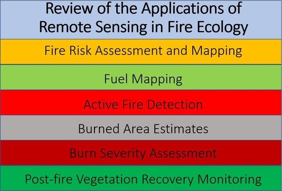
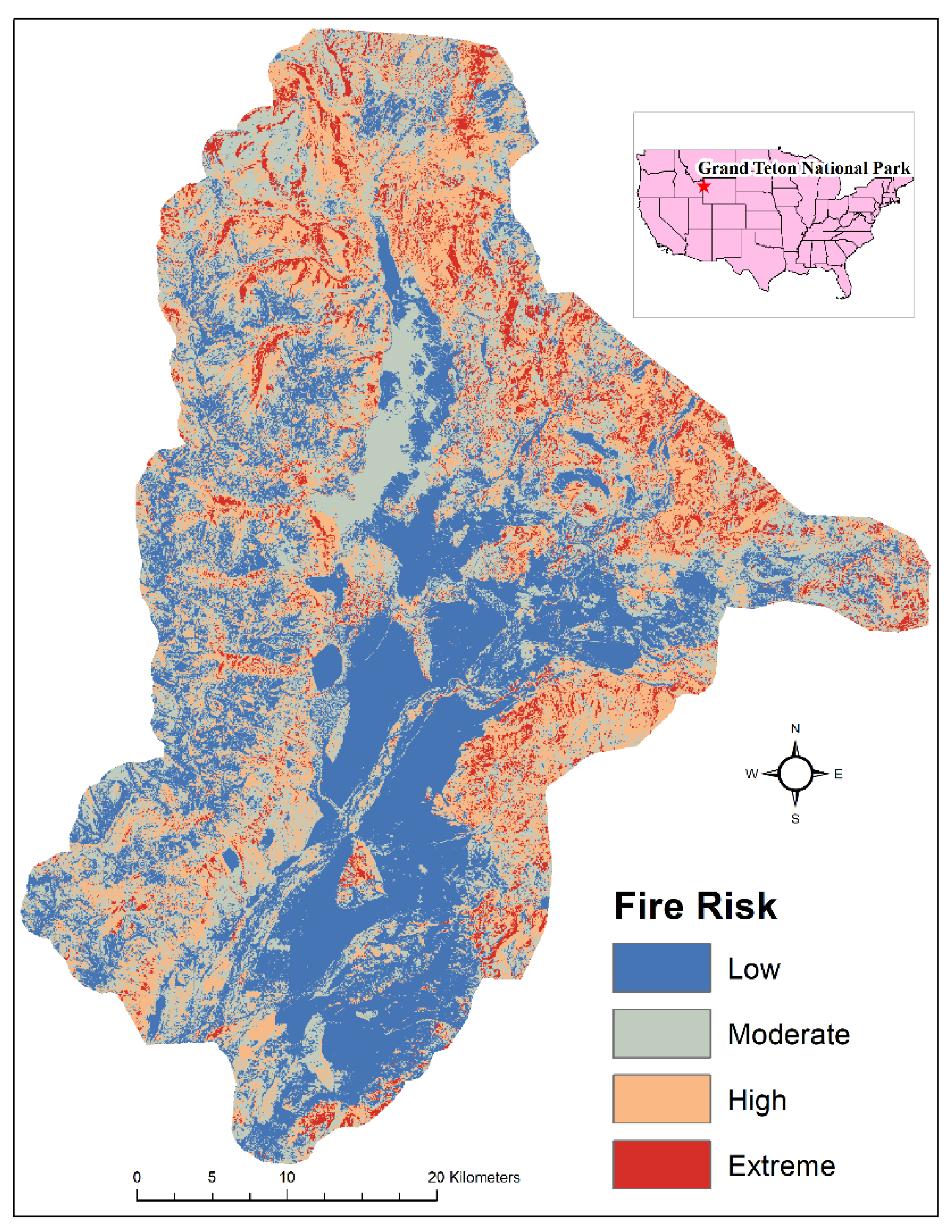
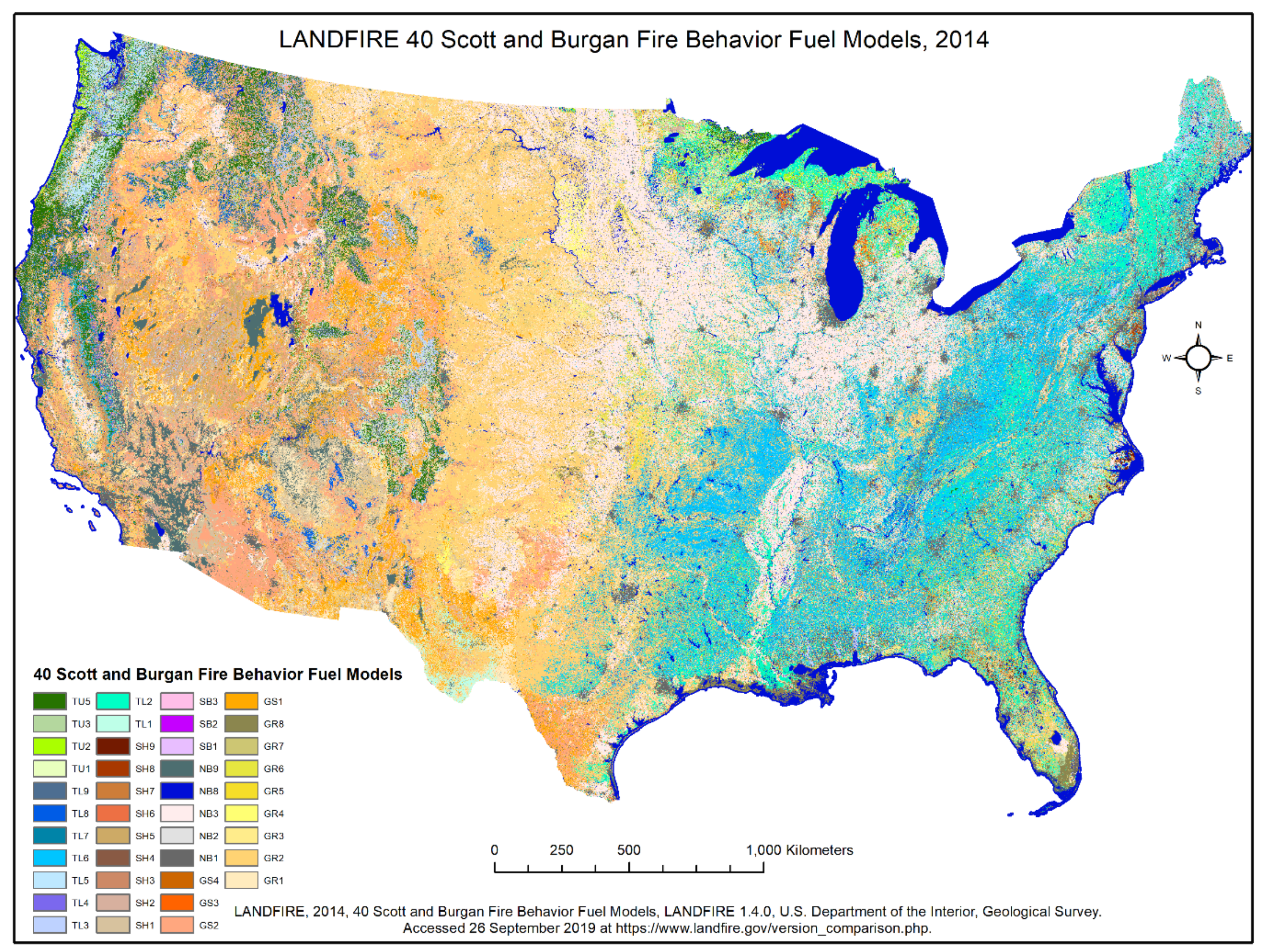
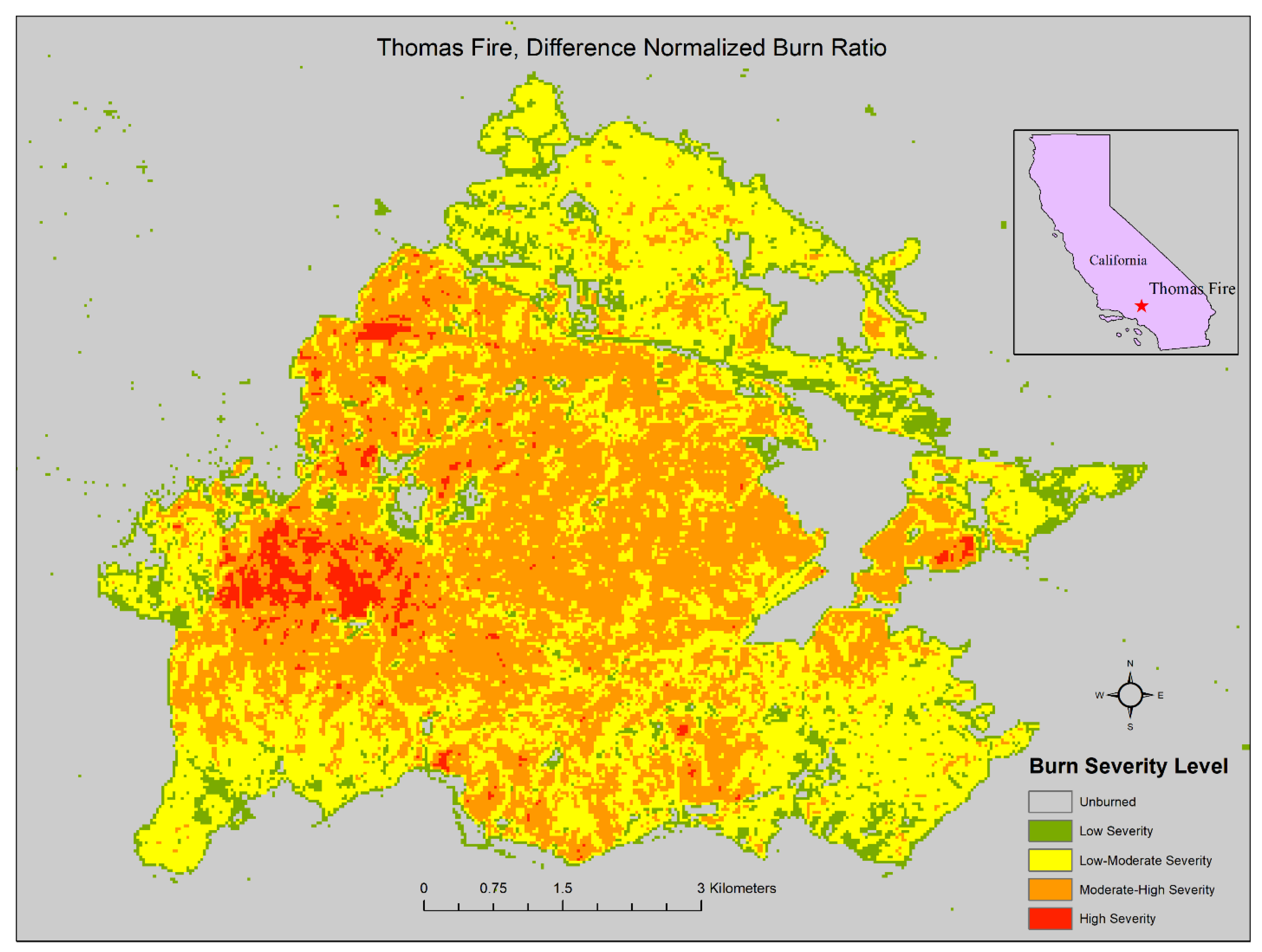
Table 1.
List of sensors commonly used in fire ecology research.
| Sensor(s) | Spatial Resolution | Advantages | Disadvantages | References |
|---|---|---|---|---|
| Landsat MSS, TM, ETM+, OLI | 15–30 * m | Free and easily accessible | Lack of canopy penetration, low temporal resolution | [13,36,37,38,39] |
| Sentinel-2 | 10–60 m | Free, relatively high spatial and temporal resolution, multiple near infrared (NIR) bands | Lack of canopy penetration | [32,40,41] |
| MODIS | 250 m–1 km | Free and easily accessible, high temporal resolution, large area analysis | Lack of canopy penetration, coarse spatial resolution limits analysis of smaller areas | [42,43,44,45,46,47,48] |
| ASTER | 15–90 m | Free and easily accessible, hyperspectral sensor, several short-wave infrared (SWIR) bands | Lack of canopy penetration, low temporal resolution | [18,21,42,49,50] |
| IKONOS | 0.8–4 m | High spatial resolution | Decommissioned, limited spectral resolution, high cost | [51,52,53,54,55] |
| AVIRIS | 4–20 m | High spatial resolution, hyperspectral sensor | High cost, complicated data processing | [38,56,57] |
| GOES | 1–4 km | High temporal resolution, large area analysis | Lack of canopy penetration, coarse spatial resolution limits fine scale analysis | [58,59,60] |
| MGS-SERIVI | 3 km | Very high temporal resolution, large area of analysis | Lack of canopy penetration, coarse spatial resolution limits fine scale analysis | [61,62,63] |
* Thermal infrared bands are collected at a coarser spatial resolution and resampled to 30 m.
Table 2.
Comparison of sensor technologies used for fuel mapping.
| Type of Sensor | Appropriate Spatial Resolution | Appropriate Temporal Resolution | Cost | Difficulty of Use |
|---|---|---|---|---|
| Geostationary Satellites | No | N/A | Free | N/A |
| Coarse Spatial Resolution (>100 m) Orbital Sensors | No | N/A | Free | N/A |
| High to Moderate Resolution (<100 m) Orbital Sensors | Yes | Yes | Free | Low |
| Lidar * | Yes | Yes | Very High ($10,000) | High |
| UAS | N/A | N/A | High ($1000) | N/A |
* Lidar is not suited for mapping surface fuel on its own but can supplement multispectral methods.
Table 3.
Comparison of technologies used for active fire detection. * Note that the appropriateness of the spatial and temporal resolutions for UASs are only appropriate if monitoring at a local scale. Also note that currently high to moderate spatial resolution sensors are not appropriate for actively detecting and monitoring active fires, but as more of these sensors become available this may change.
| Type of Sensor | Appropriate Spatial Resolution | Appropriate Temporal Resolution | Cost | Difficulty of Use |
|---|---|---|---|---|
| Geostationary Satellites | Yes | Yes | Free | Low-moderate |
| Coarse Spatial Resolution (>100 m) Orbital Sensors | Yes | Yes | Free | Low-moderate |
| High to Moderate Resolution (<100 m) Orbital Sensors | N/A | No * | Free | N/A |
| Lidar | N/A | N/A | Very High ($10,000) | N/A |
| UAS | Yes * | Yes * | High ($1000) | High |
Table 4.
Comparison of technologies for burned area estimations. * Note that high to moderate spatial resolution orbital sensors and UASs are only appropriate for burned area estimations at a local scale.
Table 4.
Comparison of technologies for burned area estimations. * Note that high to moderate spatial resolution orbital sensors and UASs are only appropriate for burned area estimations at a local scale.
| Type of Sensor | Appropriate Spatial Resolution | Appropriate Temporal Resolution | Cost | Difficulty of Use |
|---|---|---|---|---|
| Geostationary Satellites | No | N/A | Free | N/A |
| Coarse Spatial Resolution (>100 m) Orbital Sensors | Yes | Yes | Free | Low-moderate |
| High to Moderate Resolution (<100 m) Orbital Sensors | Yes * | Yes * | Free | Low |
| Lidar | N/A | N/A | Very High ($10,000) | N/A |
| UAS | Yes * | Yes * | High ($1000) | High |
Table 5.
Examples of red-edge indices that can be derived from Sentinel-2 imagery. Band numbers are based on Sentinel-2A assignments.
Table 5.
Examples of red-edge indices that can be derived from Sentinel-2 imagery. Band numbers are based on Sentinel-2A assignments.
| Red-edge Spectral Indices | Colum Equation | References |
|---|---|---|
| Chlorophyll Index red-edge | [32,151,152] | |
| Modified Simple Ratio red-edge | [32,153,154] | |
| Modified Simple Ratio red-edge narrow | ||
| Normalized Difference re-edge 1 | [32,152,154,155] | |
| Normalized Difference re-edge 1 modified | [32,155] | |
| Normalized Difference red-edge 2 | [32,152,153] | |
| Normalized Difference red-edge 2 modified | [32] | |
| Normalized Difference Vegetation Index red-edge 1 | [32] | |
| Normalized Difference Vegetation Index red-edge 1 narrow | [32] | |
| Normalized Difference Vegetation Index red-edge 2 | [32] | |
| Normalized Difference Vegetation Index red-edge 2 narrow | [32] | |
| Normalized Difference Vegetation Index red-edge 3 | [32] | |
| Normalized Difference Vegetation Index red-edge 3 narrow | [32] | |
| Simple Ratio red-edge 1 | [32] | |
| Simple Ratio red-edge 2 | [32] |
Table 6.
Comparison of technologies used for burn severity assessment. * Note that the appropriateness of the temporal resolution for high to moderate resolution sensors depends on the time of the fire compared to the next flyover by the sensor and that the appropriateness of UAS spectral resolution depends on the type of camera and the indices generated.
| Type of Sensor | Appropriate Spatial Resolution | Appropriate Temporal Resolution | Cost | Difficulty of Use |
|---|---|---|---|---|
| Geostationary Satellites | No | N/A | Free | N/A |
| Coarse Spatial Resolution (>100 m) Orbital Sensors | No | N/A | Free | N/A |
| High to Moderate Resolution (<100 m) Orbital Sensors | Yes | Yes * | Free | Low |
| Lidar | Yes | Yes | Very High ($10,000) | High |
| UAS | Yes | Yes | High ($1000) | Moderate-High |
Table 7.
Comparison of technologies used for vegetation recovery monitoring.
| Type of Sensor | Appropriate Spatial Resolution | Appropriate Temporal Resolution | Cost | Difficulty of Use |
|---|---|---|---|---|
| Geostationary Satellites | No | N/A | Free | N/A |
| Coarse Spatial Resolution (>100 m) Orbital Sensors | No | N/A | Free | N/A |
| High to Moderate Resolution (<100 m) Orbital Sensors | Yes | Yes | Free | Low |
| Lidar | Yes | Yes | Very High ($10,000) | High |
| UAS | Yes | Yes | High ($1000) | Moderate-High |
© 2019 by the authors. Licensee MDPI, Basel, Switzerland. This article is an open access article distributed under the terms and conditions of the Creative Commons Attribution (CC BY) license (http://creativecommons.org/licenses/by/4.0/).
Share and Cite
MDPI and ACS Style
Szpakowski, D.M.; Jensen, J.L.R. A Review of the Applications of Remote Sensing in Fire Ecology. Remote Sens. 2019, 11, 2638. https://0-doi-org.brum.beds.ac.uk/10.3390/rs11222638
AMA Style
Szpakowski DM, Jensen JLR. A Review of the Applications of Remote Sensing in Fire Ecology. Remote Sensing. 2019; 11(22):2638. https://0-doi-org.brum.beds.ac.uk/10.3390/rs11222638
Chicago/Turabian StyleSzpakowski, David M., and Jennifer L. R. Jensen. 2019. "A Review of the Applications of Remote Sensing in Fire Ecology" Remote Sensing 11, no. 22: 2638. https://0-doi-org.brum.beds.ac.uk/10.3390/rs11222638
Note that from the first issue of 2016, this journal uses article numbers instead of page numbers. See further details here.